Learning with sparsity-inducing norms - D©partement d'informatique
131
Learning with sparsity-inducing norms Francis Bach INRIA - Ecole Normale Sup´ erieure MLSS 2008 - Ile de R´ e, 2008
Transcript of Learning with sparsity-inducing norms - D©partement d'informatique
Learning with sparsity-inducing norms
Francis Bach
INRIA - Ecole Normale Superieure
MLSS 2008 - Ile de Re, 2008
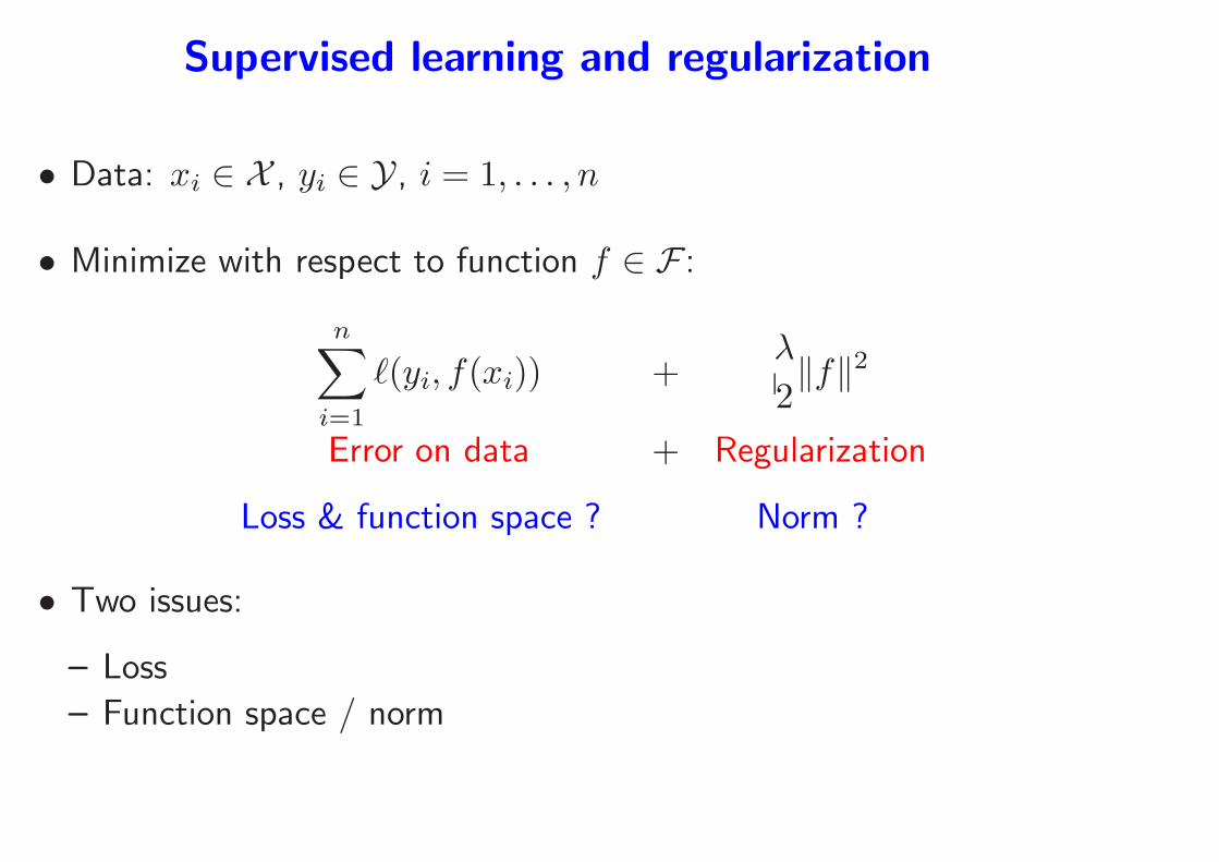
Supervised learning and regularization
• Data: xi ∈ X , yi ∈ Y, i = 1, . . . , n
• Minimize with respect to function f ∈ F :
n∑
i=1
ℓ(yi, f(xi)) +λ
2‖f‖2
Error on data + Regularization
Loss & function space ? Norm ?
• Two issues:
– Loss
– Function space / norm
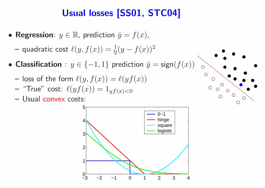
Usual losses [SS01, STC04]
• Regression: y ∈ R, prediction y = f(x),
– quadratic cost ℓ(y, f(x)) = 12(y − f(x))2
• Classification : y ∈ {−1, 1} prediction y = sign(f(x))
– loss of the form ℓ(y, f(x)) = ℓ(yf(x))
– “True” cost: ℓ(yf(x)) = 1yf(x)<0
– Usual convex costs:
−3 −2 −1 0 1 2 3 40
1
2
3
4
5
0−1hingesquarelogistic
Regularizations
• Main goal: control the “capacity” of the learning problem
• Two main lines of work
1. Use Hilbertian (RKHS) norms
– Non parametric supervised learning and kernel methods
– Well developped theory [SS01, STC04, Wah90]
2. Use “sparsity inducing” norms
– main example: ℓ1-norm ‖w‖1 =∑p
i=1 |wi|– Perform model selection as well as regularization
– Often used heuristically
• Goal of the course: Understand how and when to use sparsity-
inducing norms
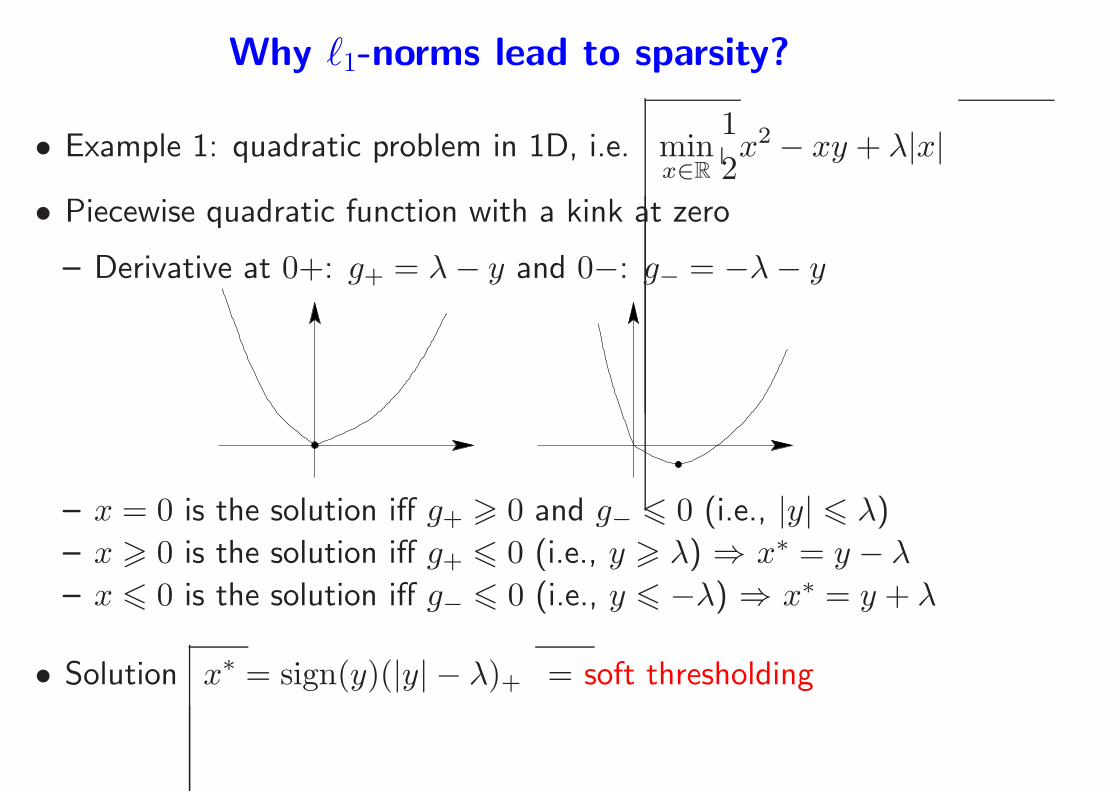
Why ℓ1-norms lead to sparsity?
• Example 1: quadratic problem in 1D, i.e. minx∈R
1
2x2 − xy + λ|x|
• Piecewise quadratic function with a kink at zero
– Derivative at 0+: g+ = λ− y and 0−: g− = −λ− y
– x = 0 is the solution iff g+ > 0 and g− 6 0 (i.e., |y| 6 λ)
– x > 0 is the solution iff g+ 6 0 (i.e., y > λ) ⇒ x∗ = y − λ– x 6 0 is the solution iff g− 6 0 (i.e., y 6 −λ) ⇒ x∗ = y + λ
• Solution x∗ = sign(y)(|y| − λ)+ = soft thresholding
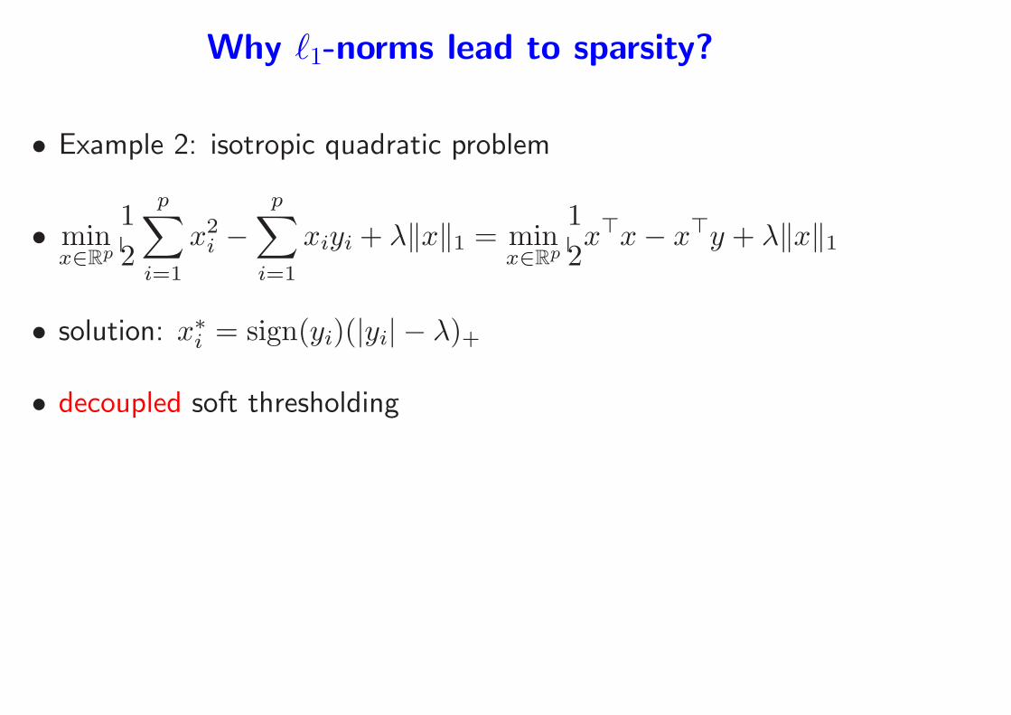
Why ℓ1-norms lead to sparsity?
• Example 2: isotropic quadratic problem
• minx∈Rp
1
2
p∑
i=1
x2i −
p∑
i=1
xiyi + λ‖x‖1 = minx∈Rp
1
2x⊤x− x⊤y + λ‖x‖1
• solution: x∗i = sign(yi)(|yi| − λ)+
• decoupled soft thresholding
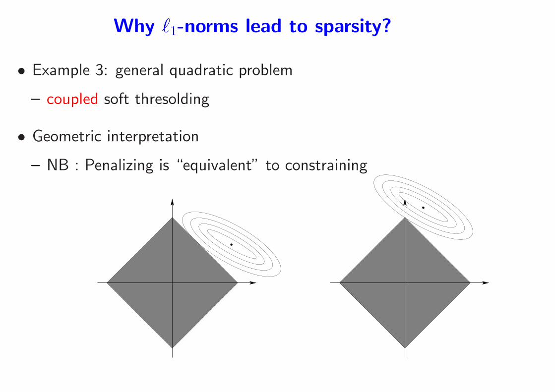
Why ℓ1-norms lead to sparsity?
• Example 3: general quadratic problem
– coupled soft thresolding
• Geometric interpretation
– NB : Penalizing is “equivalent” to constraining

Course Outline
1. ℓ1-norm regularization
• Review of nonsmooth optimization problems and algorithms
• Algorithms for the Lasso (generic or dedicated)
• Examples
2. Extensions
• Group Lasso and multiple kernel learning (MKL) + case study
• Sparse methods for matrices
• Sparse PCA
3. Theory - Consistency of pattern selection
• Low and high dimensional setting
• Links with compressed sensing
ℓ1-norm regularization
• Data: covariates xi ∈ Rp, responses yi ∈ Y, i = 1, . . . , n, given in
vector y ∈ Rp and matrix X ∈ R
n×p
• Minimize with respect to loadings/weights w ∈ Rp:
n∑
i=1
ℓ(yi, w⊤xi) + λ‖w‖1
Error on data + Regularization
• Including a constant term b?
• Assumptions on loss:
– convex and differentiable in the second variable
– NB: with the square loss ⇒ basis pursuit (signal processing)
[CDS01], Lasso (statistics/machine learning) [Tib96]
A review of nonsmooth convex
analysis and optimization
• Analysis: optimality conditions
• Optimization: algorithms
– First order methods
– Second order methods
• Books: Boyd & VandenBerghe [BV03], Bonnans et al.[BGLS03],
Nocedal & Wright [NW06], Borwein & Lewis [BL00]
Optimality conditions for ℓ1-norm regularization
• Convex differentiable problems ⇒ zero gradient!
– Example: ℓ2-regularization, i.e., minw
∑ni=1 ℓ(yi, w
⊤xi) + λ2w
⊤w
– Gradient =∑n
i=1 ℓ′(yi, w
⊤xi)xi + λw where ℓ′(yi, w⊤xi) is the
partial derivative of the loss w.r.t the second variable
– If square loss,∑n
i=1 ℓ(yi, w⊤xi) = 1
2‖y − Xw‖22 and gradient =
−X⊤(y −Xw) + λw
⇒ normal equations ⇒ w = (X⊤X + λI)−1X⊤Y
• ℓ1-norm is non differentiable!
– How to compute the gradient of the absolute value?
• WARNING - gradient methods on non smooth problems! - WARNING
⇒ Directional derivatives - subgradient
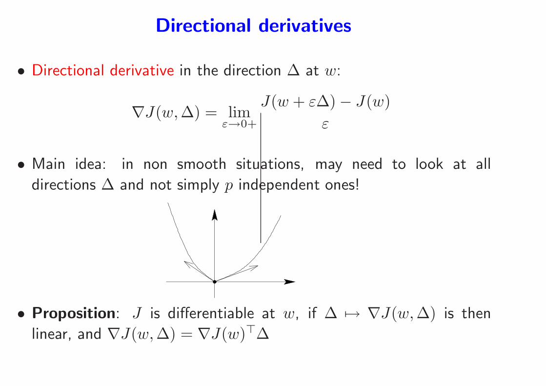
Directional derivatives
• Directional derivative in the direction ∆ at w:
∇J(w,∆) = limε→0+
J(w + ε∆)− J(w)
ε
• Main idea: in non smooth situations, may need to look at all
directions ∆ and not simply p independent ones!
• Proposition: J is differentiable at w, if ∆ 7→ ∇J(w,∆) is then
linear, and ∇J(w,∆) = ∇J(w)⊤∆
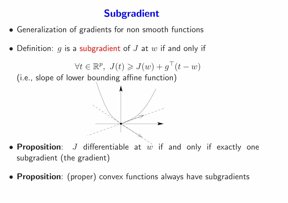
Subgradient
• Generalization of gradients for non smooth functions
• Definition: g is a subgradient of J at w if and only if
∀t ∈ Rp, J(t) > J(w) + g⊤(t− w)
(i.e., slope of lower bounding affine function)
• Proposition: J differentiable at w if and only if exactly one
subgradient (the gradient)
• Proposition: (proper) convex functions always have subgradients
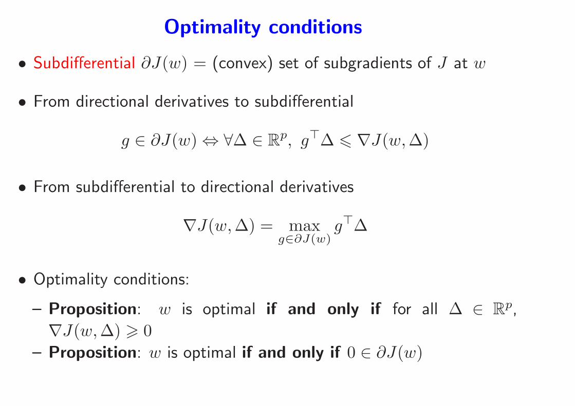
Optimality conditions
• Subdifferential ∂J(w) = (convex) set of subgradients of J at w
• From directional derivatives to subdifferential
g ∈ ∂J(w)⇔ ∀∆ ∈ Rp, g⊤∆ 6 ∇J(w,∆)
• From subdifferential to directional derivatives
∇J(w,∆) = maxg∈∂J(w)
g⊤∆
• Optimality conditions:
– Proposition: w is optimal if and only if for all ∆ ∈ Rp,
∇J(w,∆) > 0
– Proposition: w is optimal if and only if 0 ∈ ∂J(w)
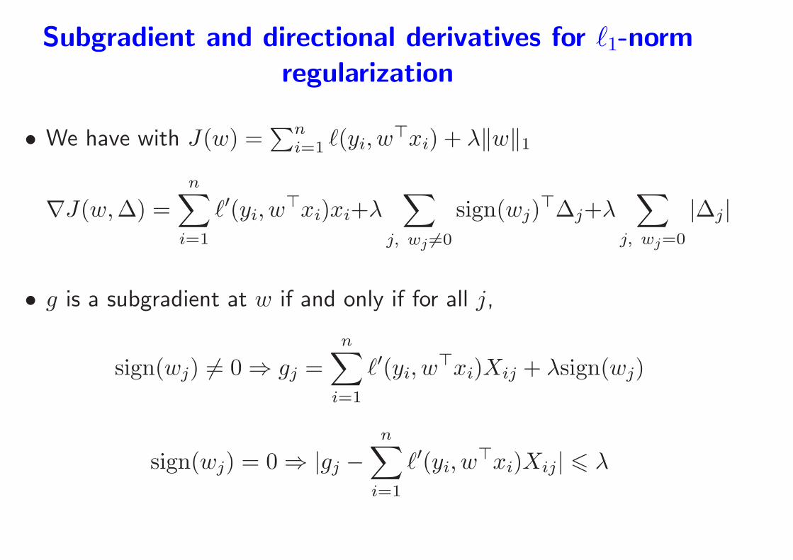
Subgradient and directional derivatives for ℓ1-norm
regularization
• We have with J(w) =∑n
i=1 ℓ(yi, w⊤xi) + λ‖w‖1
∇J(w,∆) =n∑
i=1
ℓ′(yi, w⊤xi)xi+λ
∑
j, wj 6=0
sign(wj)⊤∆j+λ
∑
j, wj=0
|∆j|
• g is a subgradient at w if and only if for all j,
sign(wj) 6= 0⇒ gj =n∑
i=1
ℓ′(yi, w⊤xi)Xij + λsign(wj)
sign(wj) = 0⇒ |gj −n∑
i=1
ℓ′(yi, w⊤xi)Xij| 6 λ
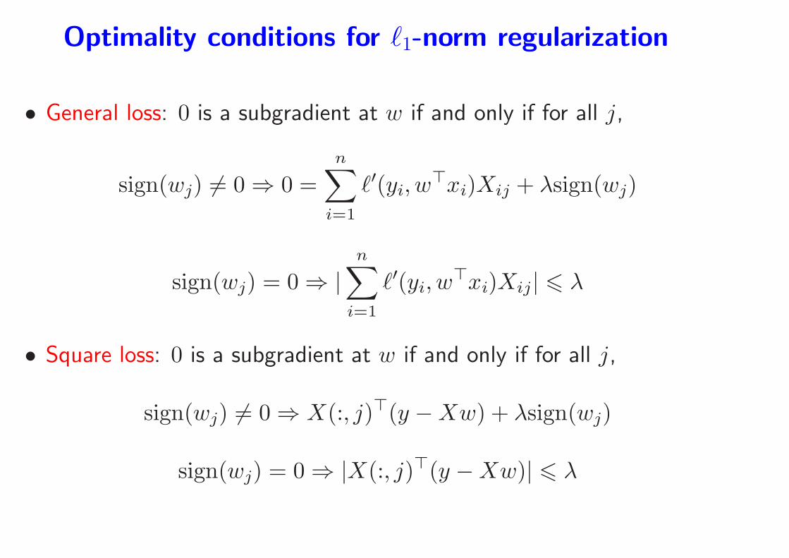
Optimality conditions for ℓ1-norm regularization
• General loss: 0 is a subgradient at w if and only if for all j,
sign(wj) 6= 0⇒ 0 =n∑
i=1
ℓ′(yi, w⊤xi)Xij + λsign(wj)
sign(wj) = 0⇒ |n∑
i=1
ℓ′(yi, w⊤xi)Xij| 6 λ
• Square loss: 0 is a subgradient at w if and only if for all j,
sign(wj) 6= 0⇒ X(:, j)⊤(y −Xw) + λsign(wj)
sign(wj) = 0⇒ |X(:, j)⊤(y −Xw)| 6 λ
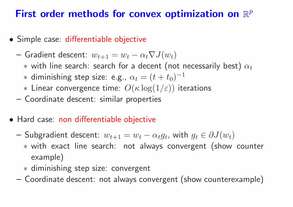
First order methods for convex optimization on Rp
• Simple case: differentiable objective
– Gradient descent: wt+1 = wt − αt∇J(wt)
∗ with line search: search for a decent (not necessarily best) αt
∗ diminishing step size: e.g., αt = (t+ t0)−1
∗ Linear convergence time: O(κ log(1/ε)) iterations
– Coordinate descent: similar properties
• Hard case: non differentiable objective
– Subgradient descent: wt+1 = wt − αtgt, with gt ∈ ∂J(wt)
∗ with exact line search: not always convergent (show counter
example)
∗ diminishing step size: convergent
– Coordinate descent: not always convergent (show counterexample)
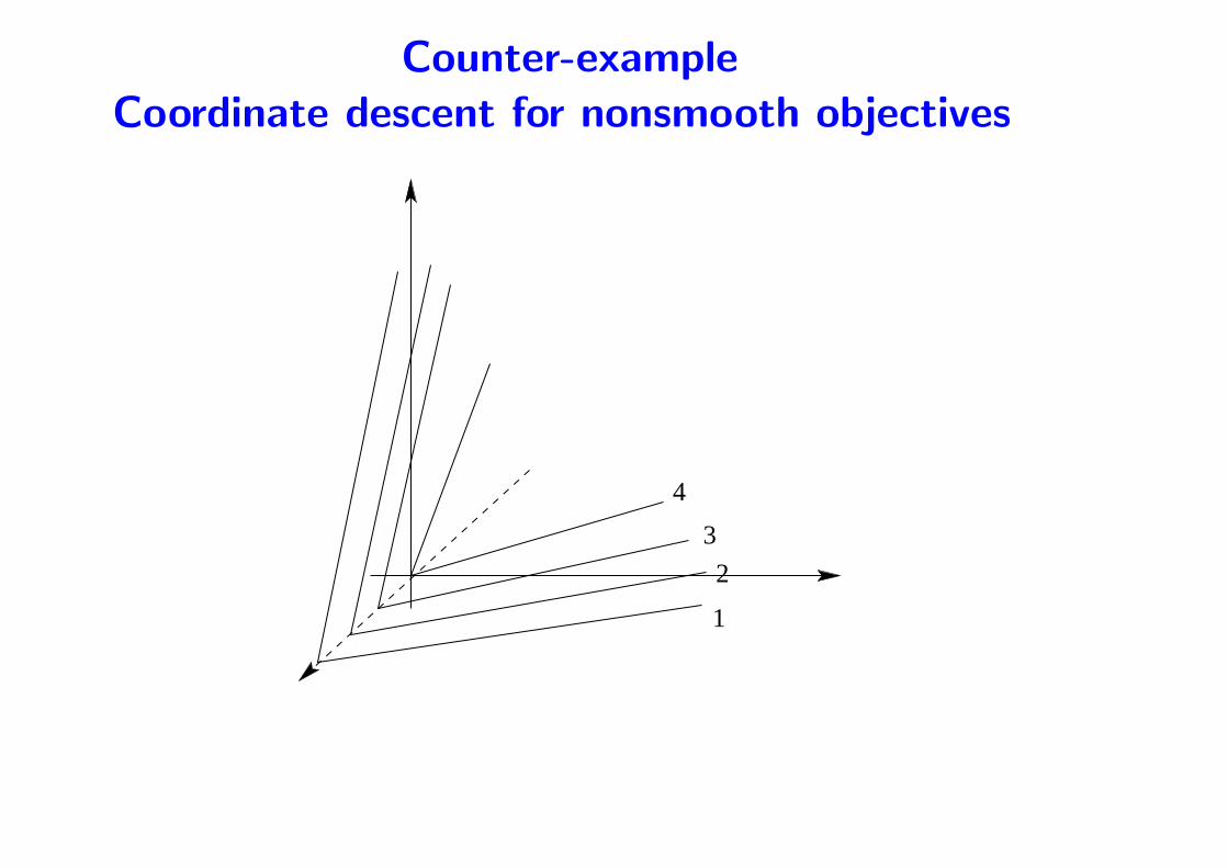
Counter-example
Coordinate descent for nonsmooth objectives
4
1
2
3
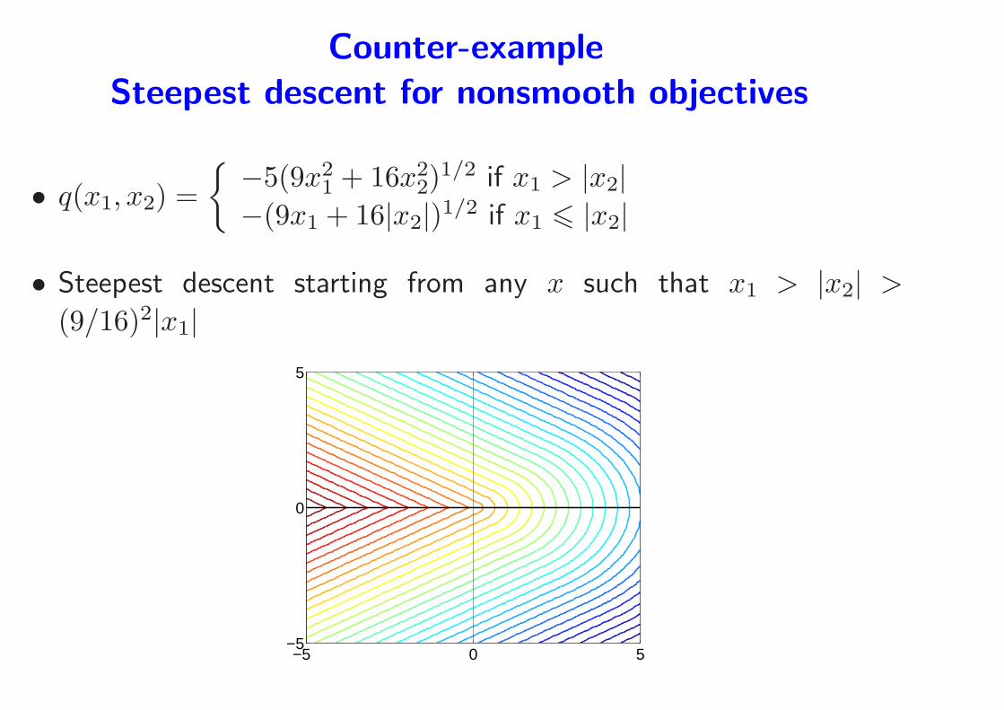
Counter-example
Steepest descent for nonsmooth objectives
• q(x1, x2) =
{ −5(9x21 + 16x2
2)1/2 if x1 > |x2|
−(9x1 + 16|x2|)1/2 if x1 6 |x2|
• Steepest descent starting from any x such that x1 > |x2| >(9/16)2|x1|
−5 0 5−5
0
5
Second order methods
• Differentiable case
– Newton: wt+1 = wt − αtH−1t gt
∗ Traditional: αt = 1, but non globally convergent
∗ globally convergent with line search for αt (see Boyd, 2003)
∗ O(log log(1/ε)) (slower) iterations
– Quasi-newton methods (see Bonnans et al., 2003)
• Non differentiable case (interior point methods)
– Smoothing of problem + second order methods
∗ See example later and (Boyd, 2003)
∗ Theoretically O(√p) Newton steps, usually O(1) Newton steps
First order or second order methods for machine
learning?
• objecive defined as average (i.e., up to n−1/2): no need to optimize
up to 10−16!
– Second-order: slower but worryless
– First-order: faster but care must be taken regarding convergence
• Rule of thumb
– Small scale ⇒ second order
– Large scale ⇒ first order
– Unless dedicated algorithm using structure (like for the Lasso)
• See Bottou & Bousquet (2008) [BB08] for further details
Algorithms for ℓ1-norms:
Gaussian hare vs. Laplacian tortoise
Cheap (and not dirty) algorithms for all losses
• Coordinate descent [WL08]
– Globaly convergent here under reasonable assumptions!
– very fast updates
• Subgradient descent
• Smoothing the absolute value + first/second order methods
– Replace |wi| by (w2i + ε2i )
1/2
– Use gradient descent or Newton with diminishing ε
• More dedicated algorithms to get the best of both worlds: fast and
precise
Special case of square loss
• Quadratic programming formulation: minimize
1
2‖y−Xw‖2+λ
p∑
j=1
(w+j +w−
j ) such that w = w+−w−, w+> 0, w−
> 0
– generic toolboxes ⇒ very slow
• Main property: if the sign pattern s ∈ {−1, 0, 1}p of the solution is
known, the solution can be obtained in closed form
– Lasso equivalent to minimizing 12‖y−XJwJ‖2 + λs⊤JwJ w.r.t. wJ
where J = {j, sj 6= 0}.– Closed form solution wJ = (X⊤
J XJ)−1(X⊤J Y + λsJ)
• “Simply” need to check that sign(wJ) = sJ and optimality for Jc
Optimality conditions for the Lasso
• 0 is a subgradient at w if and only if for all j,
– Active variable condition
sign(wj) 6= 0⇒ X(:, j)⊤(y −Xw) + λsign(wj)
NB: allows to compute wJ
– Inactive variable condition
sign(wj) = 0⇒ |X(:, j)⊤(y −Xw)| 6 λ
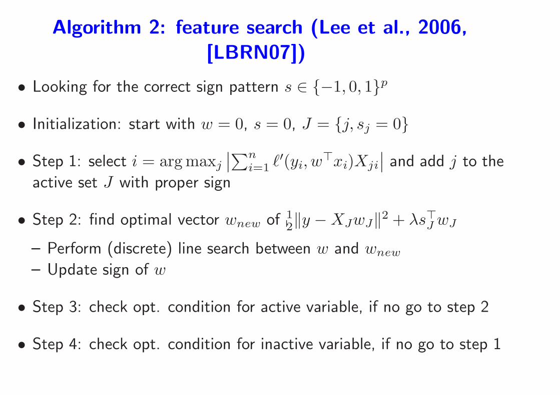
Algorithm 2: feature search (Lee et al., 2006,
[LBRN07])
• Looking for the correct sign pattern s ∈ {−1, 0, 1}p
• Initialization: start with w = 0, s = 0, J = {j, sj = 0}
• Step 1: select i = arg maxj
∣
∣
∑ni=1 ℓ
′(yi, w⊤xi)Xji
∣
∣ and add j to the
active set J with proper sign
• Step 2: find optimal vector wnew of 12‖y −XJwJ‖2 + λs⊤JwJ
– Perform (discrete) line search between w and wnew
– Update sign of w
• Step 3: check opt. condition for active variable, if no go to step 2
• Step 4: check opt. condition for inactive variable, if no go to step 1
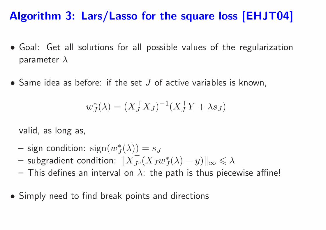
Algorithm 3: Lars/Lasso for the square loss [EHJT04]
• Goal: Get all solutions for all possible values of the regularization
parameter λ
• Same idea as before: if the set J of active variables is known,
w∗J(λ) = (X⊤
J XJ)−1(X⊤J Y + λsJ)
valid, as long as,
– sign condition: sign(w∗J(λ)) = sJ
– subgradient condition: ‖X⊤Jc(XJw
∗J(λ)− y)‖∞ 6 λ
– This defines an interval on λ: the path is thus piecewise affine!
• Simply need to find break points and directions
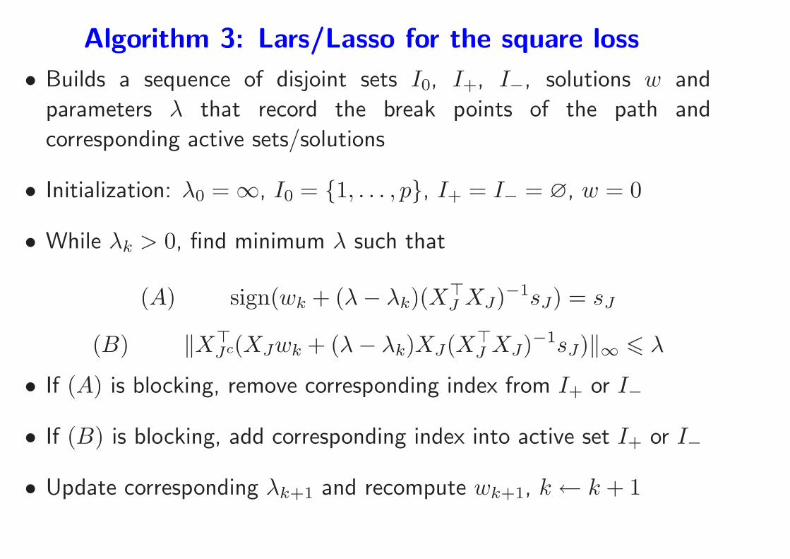
Algorithm 3: Lars/Lasso for the square loss
• Builds a sequence of disjoint sets I0, I+, I−, solutions w and
parameters λ that record the break points of the path and
corresponding active sets/solutions
• Initialization: λ0 =∞, I0 = {1, . . . , p}, I+ = I− = ∅, w = 0
• While λk > 0, find minimum λ such that
(A) sign(wk + (λ− λk)(X⊤J XJ)−1sJ) = sJ
(B) ‖X⊤Jc(XJwk + (λ− λk)XJ(X⊤
J XJ)−1sJ)‖∞ 6 λ
• If (A) is blocking, remove corresponding index from I+ or I−
• If (B) is blocking, add corresponding index into active set I+ or I−
• Update corresponding λk+1 and recompute wk+1, k ← k + 1
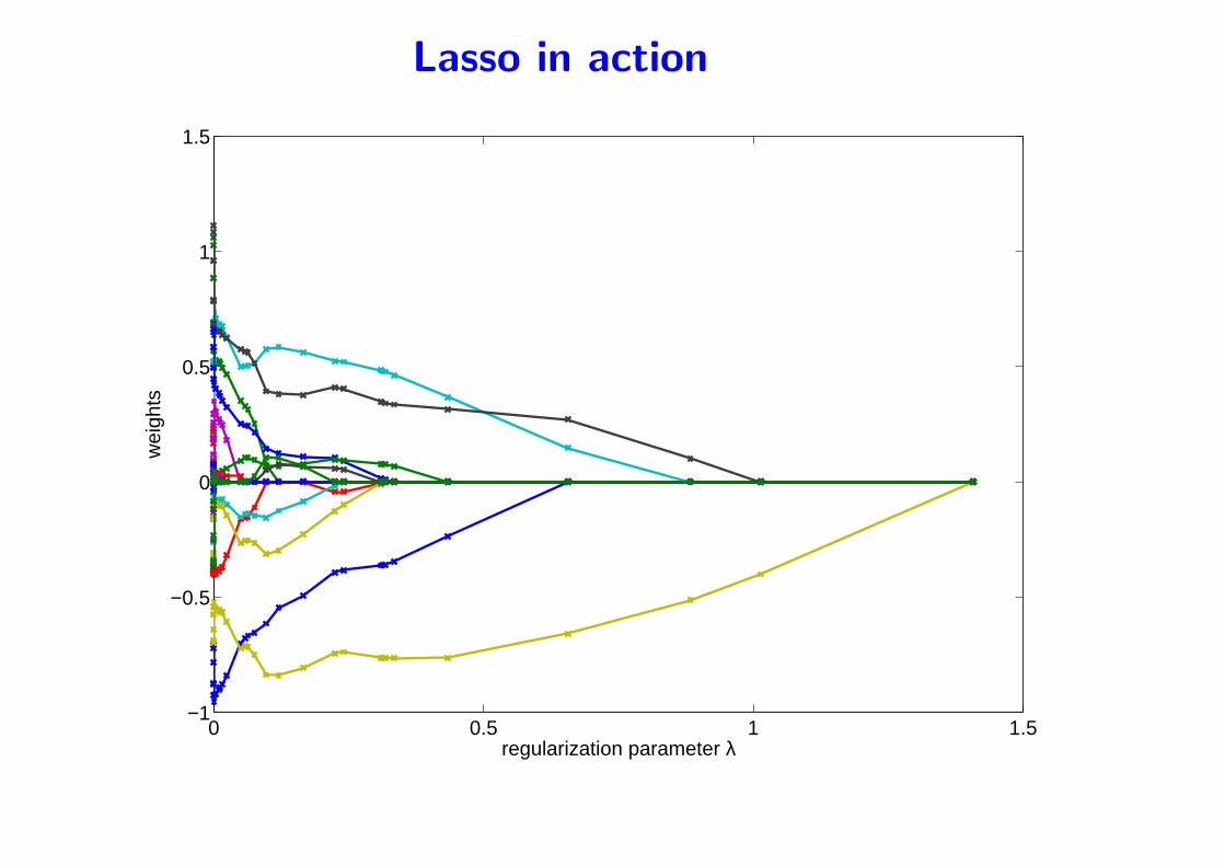
Lasso in action
• Piecewise linear paths
• When is it supposed to work?
– Show simulations with random Gaussians, regularization parameter
estimated by cross-validation
– sparsity is expected or not
Lasso in action
0 0.5 1 1.5−1
−0.5
0
0.5
1
1.5
regularization parameter λ
wei
ghts
Comparing Lasso and other strategies for linear
regression and subset selection
• Compared methods to reach the least-square solution [HTF01]
– Ridge regression: minw12‖y −Xw‖22 + λ
2‖w‖22– Lasso: minw
12‖y −Xw‖22 + λ‖w‖1
– Forward greedy:
∗ Initialization with empty set
∗ Sequentially add the variable that best reduces the square loss
• Each method builds a path of solutions from 0 to wOLS
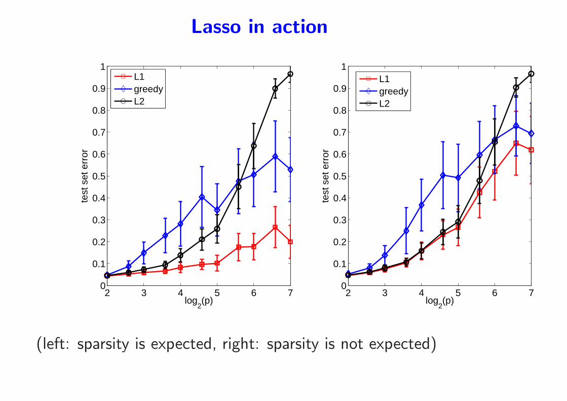
Lasso in action
2 3 4 5 6 70
0.1
0.2
0.3
0.4
0.5
0.6
0.7
0.8
0.9
1
log2(p)
test
set
err
or
2 3 4 5 6 70
0.1
0.2
0.3
0.4
0.5
0.6
0.7
0.8
0.9
1
log2(p)
test
set
err
or
L1greedyL2
L1greedyL2
(left: sparsity is expected, right: sparsity is not expected)
ℓ1-norm regularization and sparsity
Summary
• Nonsmooth optimization
– subgradient, directional derivatives
– descent methods might not always work
– first/second order methods
• Algorithms
– Cheap algorithms for all losses
– Dedicated path algorithm for the square loss

Course Outline
1. ℓ1-norm regularization
• Review of nonsmooth optimization problems and algorithms
• Algorithms for the Lasso (generic or dedicated)
• Examples
2. Extensions
• Group Lasso and multiple kernel learning (MKL) + case study
• Sparse methods for matrices
• Sparse PCA
3. Theory - Consistency of pattern selection
• Low and high dimensional setting
• Links with compressed sensing
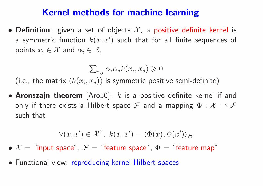
Kernel methods for machine learning
• Definition: given a set of objects X , a positive definite kernel is
a symmetric function k(x, x′) such that for all finite sequences of
points xi ∈ X and αi ∈ R,
∑
i,j αiαjk(xi, xj) > 0
(i.e., the matrix (k(xi, xj)) is symmetric positive semi-definite)
• Aronszajn theorem [Aro50]: k is a positive definite kernel if and
only if there exists a Hilbert space F and a mapping Φ : X 7→ Fsuch that
∀(x, x′) ∈ X 2, k(x, x′) = 〈Φ(x),Φ(x′)〉H• X = “input space”, F = “feature space”, Φ = “feature map”
• Functional view: reproducing kernel Hilbert spaces
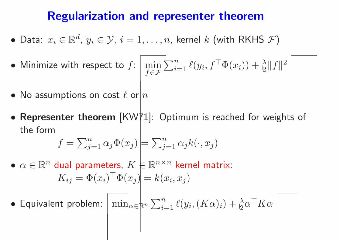
Regularization and representer theorem
• Data: xi ∈ Rd, yi ∈ Y, i = 1, . . . , n, kernel k (with RKHS F)
• Minimize with respect to f : minf∈F
∑ni=1 ℓ(yi, f
⊤Φ(xi)) + λ2‖f‖2
• No assumptions on cost ℓ or n
• Representer theorem [KW71]: Optimum is reached for weights of
the form
f =∑n
j=1αjΦ(xj) =∑n
j=1αjk(·, xj)
• α ∈ Rn dual parameters, K ∈ R
n×n kernel matrix:
Kij = Φ(xi)⊤Φ(xj) = k(xi, xj)
• Equivalent problem: minα∈Rn∑n
i=1 ℓ(yi, (Kα)i) + λ2α
⊤Kα

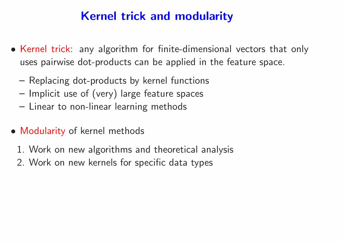
Kernel trick and modularity
• Kernel trick: any algorithm for finite-dimensional vectors that only
uses pairwise dot-products can be applied in the feature space.
– Replacing dot-products by kernel functions
– Implicit use of (very) large feature spaces
– Linear to non-linear learning methods
Kernel trick and modularity
• Kernel trick: any algorithm for finite-dimensional vectors that only
uses pairwise dot-products can be applied in the feature space.
– Replacing dot-products by kernel functions
– Implicit use of (very) large feature spaces
– Linear to non-linear learning methods
• Modularity of kernel methods
1. Work on new algorithms and theoretical analysis
2. Work on new kernels for specific data types
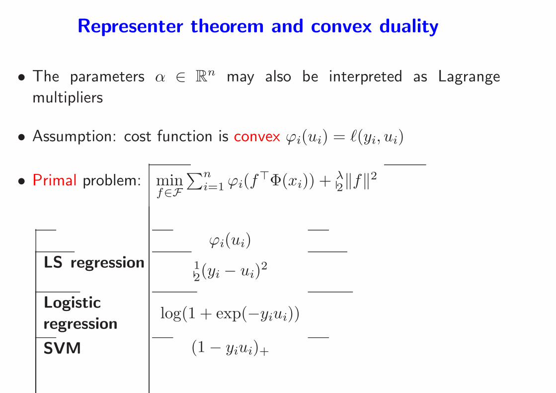
Representer theorem and convex duality
• The parameters α ∈ Rn may also be interpreted as Lagrange
multipliers
• Assumption: cost function is convex ϕi(ui) = ℓ(yi, ui)
• Primal problem: minf∈F
∑ni=1ϕi(f
⊤Φ(xi)) + λ2‖f‖2
ϕi(ui)
LS regression 12(yi − ui)
2
Logistic
regressionlog(1 + exp(−yiui))
SVM (1− yiui)+
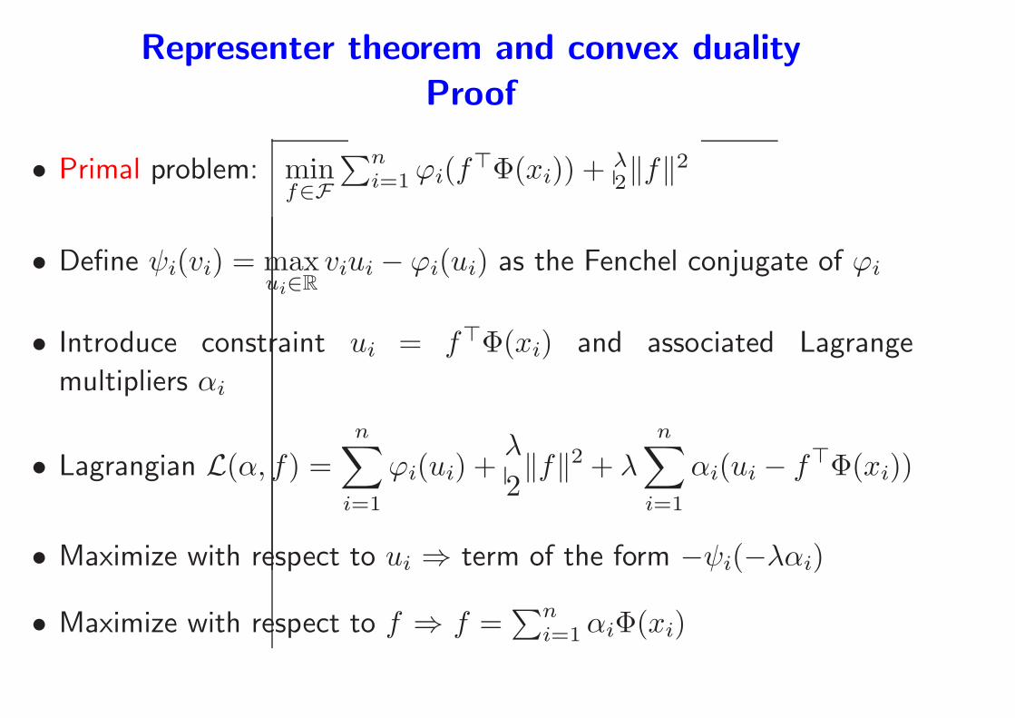
Representer theorem and convex duality
Proof
• Primal problem: minf∈F
∑ni=1ϕi(f
⊤Φ(xi)) + λ2‖f‖2
• Define ψi(vi) = maxui∈R
viui − ϕi(ui) as the Fenchel conjugate of ϕi
• Introduce constraint ui = f⊤Φ(xi) and associated Lagrange
multipliers αi
• Lagrangian L(α, f) =n∑
i=1
ϕi(ui) +λ
2‖f‖2 + λ
n∑
i=1
αi(ui − f⊤Φ(xi))
• Maximize with respect to ui ⇒ term of the form −ψi(−λαi)
• Maximize with respect to f ⇒ f =∑n
i=1αiΦ(xi)
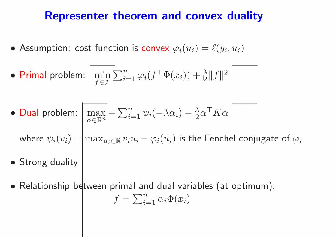
Representer theorem and convex duality
• Assumption: cost function is convex ϕi(ui) = ℓ(yi, ui)
• Primal problem: minf∈F
∑ni=1ϕi(f
⊤Φ(xi)) + λ2‖f‖2
• Dual problem: maxα∈Rn
−∑ni=1ψi(−λαi)− λ
2α⊤Kα
where ψi(vi) = maxui∈R viui−ϕi(ui) is the Fenchel conjugate of ϕi
• Strong duality
• Relationship between primal and dual variables (at optimum):
f =∑n
i=1αiΦ(xi)
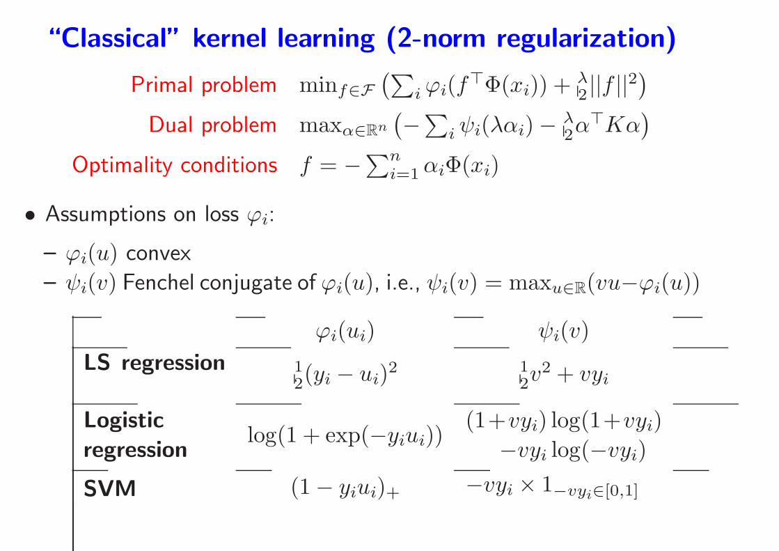
“Classical” kernel learning (2-norm regularization)
Primal problem minf∈F
(∑
iϕi(f⊤Φ(xi)) + λ
2 ||f ||2)
Dual problem maxα∈Rn
(
−∑iψi(λαi)− λ2α
⊤Kα)
Optimality conditions f = −∑ni=1αiΦ(xi)
• Assumptions on loss ϕi:
– ϕi(u) convex
– ψi(v) Fenchel conjugate of ϕi(u), i.e., ψi(v) = maxu∈R(vu−ϕi(u))
ϕi(ui) ψi(v)
LS regression 12(yi − ui)
2 12v
2 + vyi
Logistic
regressionlog(1 + exp(−yiui))
(1+vyi) log(1+vyi)
−vyi log(−vyi)
SVM (1− yiui)+ −vyi × 1−vyi∈[0,1]
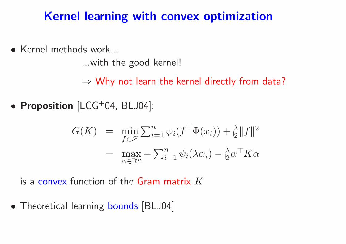
Kernel learning with convex optimization
• Kernel methods work...
...with the good kernel!
⇒ Why not learn the kernel directly from data?
Kernel learning with convex optimization
• Kernel methods work...
...with the good kernel!
⇒ Why not learn the kernel directly from data?
• Proposition [LCG+04, BLJ04]:
G(K) = minf∈F
∑ni=1ϕi(f
⊤Φ(xi)) + λ2‖f‖2
= maxα∈Rn
−∑ni=1ψi(λαi)− λ
2α⊤Kα
is a convex function of the Gram matrix K
• Theoretical learning bounds [BLJ04]
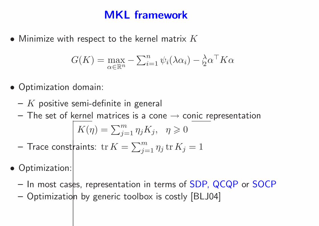
MKL framework
• Minimize with respect to the kernel matrix K
G(K) = maxα∈Rn
−∑ni=1ψi(λαi)− λ
2α⊤Kα
• Optimization domain:
– K positive semi-definite in general
– The set of kernel matrices is a cone → conic representation
K(η) =∑m
j=1 ηjKj, η > 0
– Trace constraints: trK =∑m
j=1 ηj trKj = 1
• Optimization:
– In most cases, representation in terms of SDP, QCQP or SOCP
– Optimization by generic toolbox is costly [BLJ04]
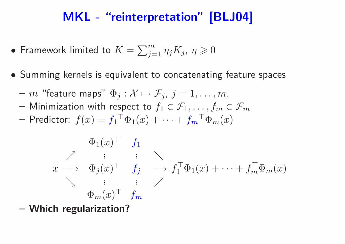
MKL - “reinterpretation” [BLJ04]
• Framework limited to K =∑m
j=1 ηjKj, η > 0
• Summing kernels is equivalent to concatenating feature spaces
– m “feature maps” Φj : X 7→ Fj, j = 1, . . . ,m.
– Minimization with respect to f1 ∈ F1, . . . , fm ∈ Fm
– Predictor: f(x) = f1⊤Φ1(x) + · · ·+ fm
⊤Φm(x)
x
Φ1(x)⊤ f1
ր ... ... ց−→ Φj(x)
⊤ fj −→ց ... ... ր
Φm(x)⊤ fm
f⊤1 Φ1(x) + · · ·+ f⊤mΦm(x)
– Which regularization?
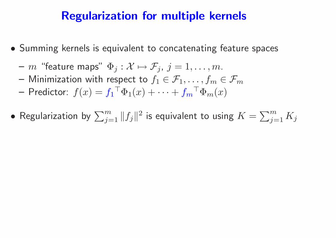
Regularization for multiple kernels
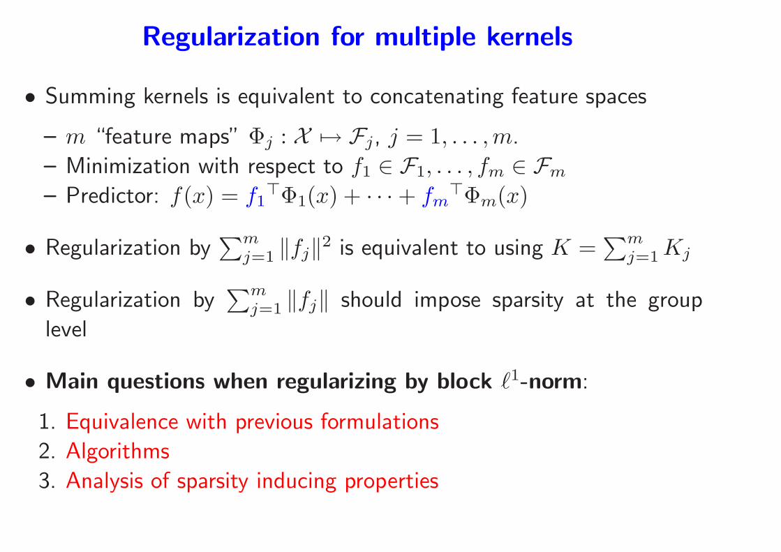
• Summing kernels is equivalent to concatenating feature spaces
– m “feature maps” Φj : X 7→ Fj, j = 1, . . . ,m.
– Minimization with respect to f1 ∈ F1, . . . , fm ∈ Fm
– Predictor: f(x) = f1⊤Φ1(x) + · · ·+ fm
⊤Φm(x)
• Regularization by∑m
j=1 ‖fj‖2 is equivalent to using K =∑m
j=1Kj
Regularization for multiple kernels
• Summing kernels is equivalent to concatenating feature spaces
– m “feature maps” Φj : X 7→ Fj, j = 1, . . . ,m.
– Minimization with respect to f1 ∈ F1, . . . , fm ∈ Fm
– Predictor: f(x) = f1⊤Φ1(x) + · · ·+ fm
⊤Φm(x)
• Regularization by∑m
j=1 ‖fj‖2 is equivalent to using K =∑m
j=1Kj
• Regularization by∑m
j=1 ‖fj‖ should impose sparsity at the group
level
• Main questions when regularizing by block ℓ1-norm:
1. Equivalence with previous formulations
2. Algorithms
3. Analysis of sparsity inducing properties
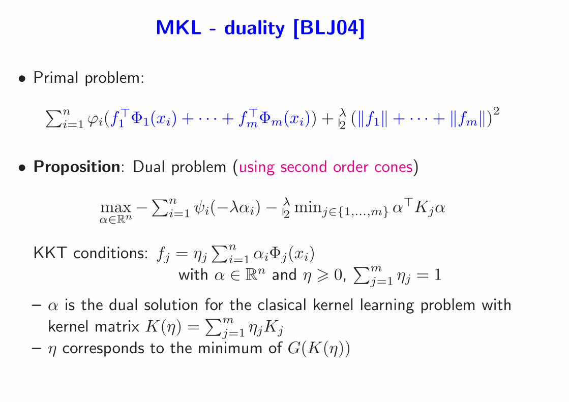
MKL - duality [BLJ04]
• Primal problem:
∑ni=1ϕi(f
⊤1 Φ1(xi) + · · ·+ f⊤mΦm(xi)) + λ
2 (‖f1‖+ · · ·+ ‖fm‖)2
• Proposition: Dual problem (using second order cones)
maxα∈Rn
−∑ni=1ψi(−λαi)− λ
2 minj∈{1,...,m}α⊤Kjα
KKT conditions: fj = ηj
∑ni=1αiΦj(xi)
with α ∈ Rn and η > 0,
∑mj=1 ηj = 1
– α is the dual solution for the clasical kernel learning problem with
kernel matrix K(η) =∑m
j=1 ηjKj
– η corresponds to the minimum of G(K(η))
Algorithms for MKL
• (very) costly optimization with SDP, QCQP ou SOCP
– n > 1, 000− 10, 000, m > 100 not possible
– “loose” required precision ⇒ first order methods
• Dual coordinate ascent (SMO) with smoothing [BLJ04]
• Optimization of G(K) by cutting planes [SRSS06]
• Optimization of G(K) with steepest descent with smoothing
[RBCG08]
• Regularization path [BTJ04]
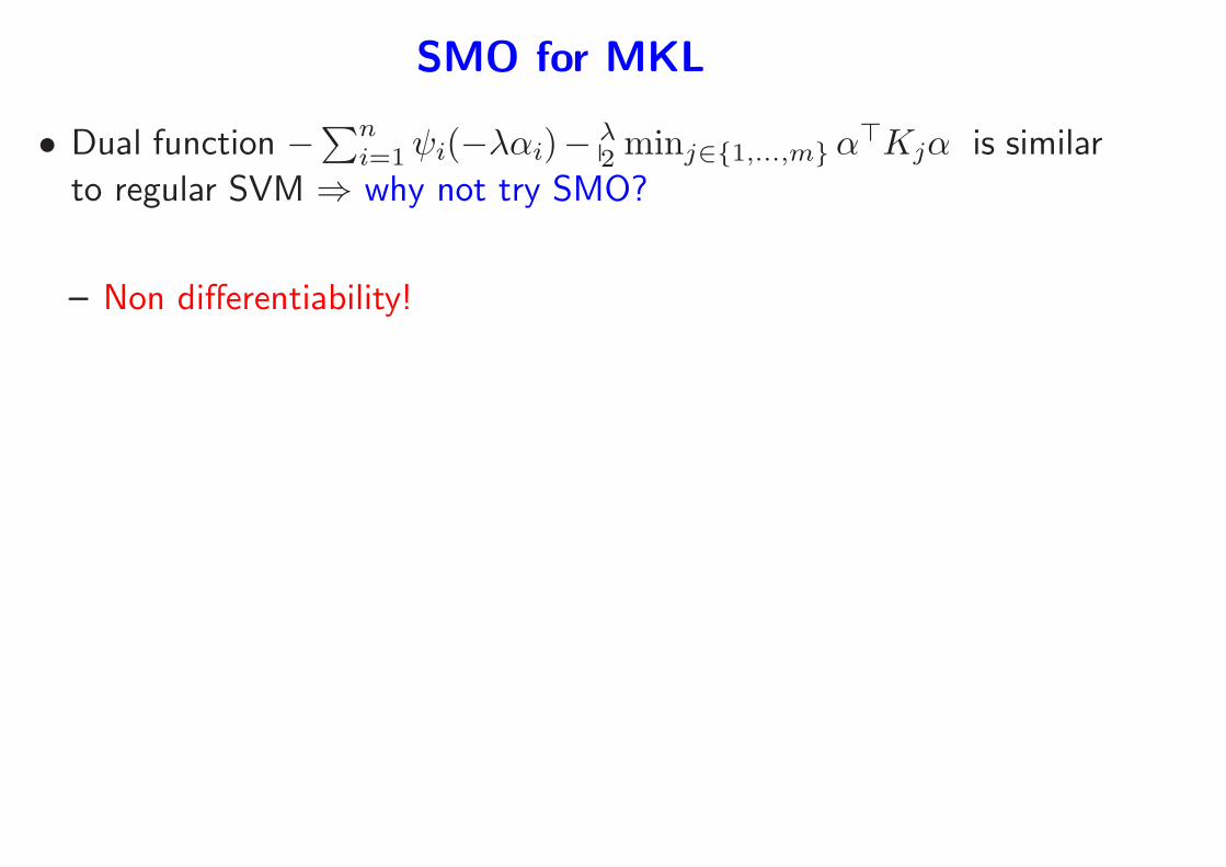
SMO for MKL [BLJ04]
• Dual function −∑ni=1ψi(−λαi)− λ
2 minj∈{1,...,m}α⊤Kjα is similar
to regular SVM ⇒ why not try SMO?
SMO for MKL
• Dual function −∑ni=1ψi(−λαi)− λ
2 minj∈{1,...,m}α⊤Kjα is similar
to regular SVM ⇒ why not try SMO?
– Non differentiability!
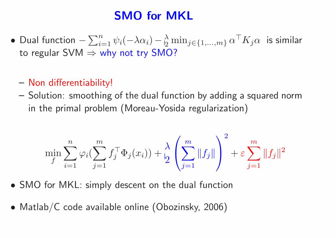
SMO for MKL
• Dual function −∑ni=1ψi(−λαi)− λ
2 minj∈{1,...,m}α⊤Kjα is similar
to regular SVM ⇒ why not try SMO?
– Non differentiability!
– Solution: smoothing of the dual function by adding a squared norm
in the primal problem (Moreau-Yosida regularization)
minf
n∑
i=1
ϕi(m∑
j=1
f⊤j Φj(xi)) +λ
2
m∑
j=1
‖fj‖
2
+ εm∑
j=1
‖fj‖2
• SMO for MKL: simply descent on the dual function
• Matlab/C code available online (Obozinsky, 2006)
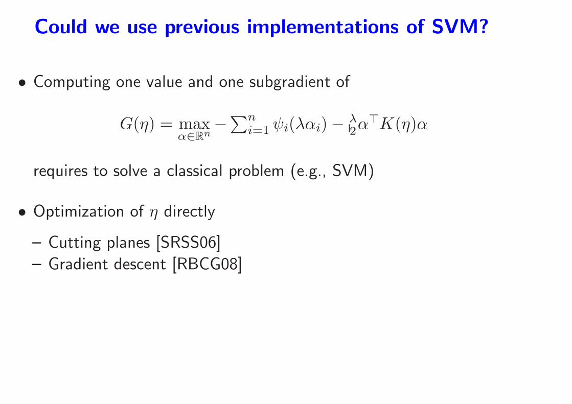
Could we use previous implementations of SVM?
• Computing one value and one subgradient of
G(η) = maxα∈Rn
−∑ni=1ψi(λαi)− λ
2α⊤K(η)α
requires to solve a classical problem (e.g., SVM)
• Optimization of η directly
– Cutting planes [SRSS06]
– Gradient descent [RBCG08]
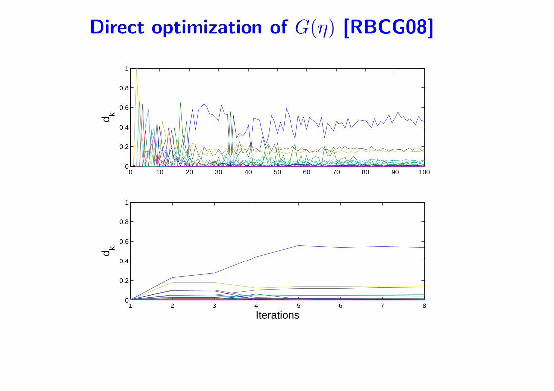
Direct optimization of G(η) [RBCG08]
0 10 20 30 40 50 60 70 80 90 1000
0.2
0.4
0.6
0.8
1
d k
1 2 3 4 5 6 7 80
0.2
0.4
0.6
0.8
1
Iterations
d k
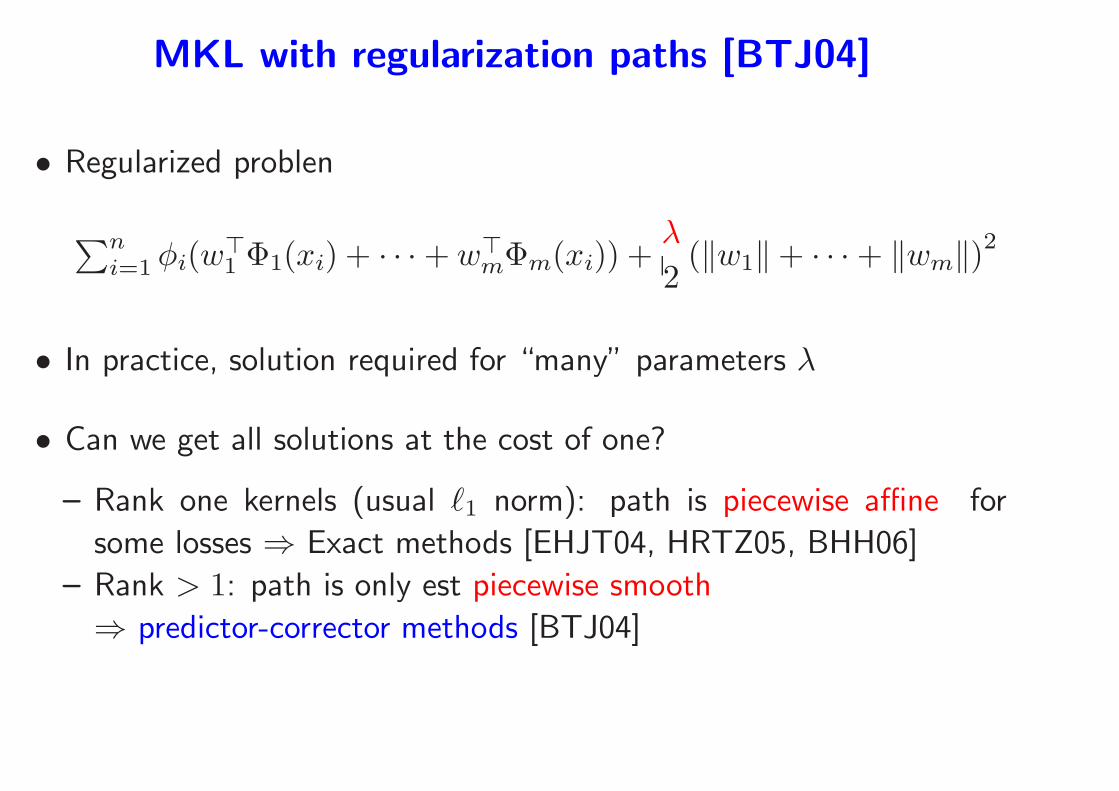
MKL with regularization paths [BTJ04]
• Regularized problen
∑ni=1 φi(w
⊤1 Φ1(xi) + · · ·+ w⊤
mΦm(xi)) +λ
2(‖w1‖+ · · ·+ ‖wm‖)2
• In practice, solution required for “many” parameters λ
• Can we get all solutions at the cost of one?
– Rank one kernels (usual ℓ1 norm): path is piecewise affine for
some losses ⇒ Exact methods [EHJT04, HRTZ05, BHH06]
– Rank > 1: path is only est piecewise smooth
⇒ predictor-corrector methods [BTJ04]
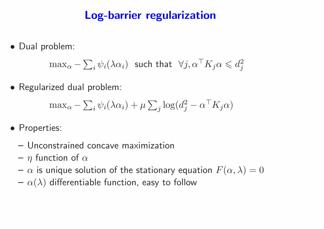
Log-barrier regularization
• Dual problem:
maxα−∑
iψi(λαi) such that ∀j, α⊤Kjα 6 d2j
• Regularized dual problem:
maxα−∑
iψi(λαi) + µ∑
j log(d2j − α⊤Kjα)
• Properties:
– Unconstrained concave maximization
– η function of α
– α is unique solution of the stationary equation F (α, λ) = 0
– α(λ) differentiable function, easy to follow
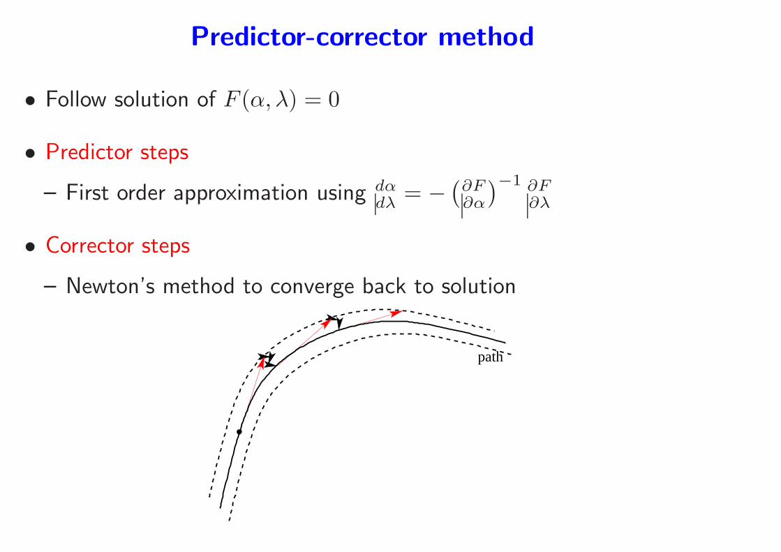
Predictor-corrector method
• Follow solution of F (α, λ) = 0
• Predictor steps
– First order approximation using dαdλ = −
(
∂F∂α
)−1 ∂F∂λ
• Corrector steps
– Newton’s method to converge back to solution
path
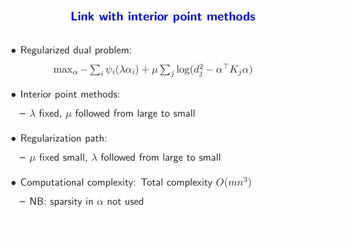
Link with interior point methods
• Regularized dual problem:
maxα−∑
iψi(λαi) + µ∑
j log(d2j − α⊤Kjα)
• Interior point methods:
– λ fixed, µ followed from large to small
• Regularization path:
– µ fixed small, λ followed from large to small
• Computational complexity: Total complexity O(mn3)
– NB: sparsity in α not used
Applications
• Bioinformatics [LBC+04]
– Protein function prediction
– Heterogeneous data sources
∗ Amino acid sequences
∗ Protein-protein interactions
∗ Genetic interactions
∗ Gene expression measurements
• Image annotation [HB07]
A case study in kernel methods
• Goal: show how to use kernel methods (kernel design + kernel
learning) on a “real problem”

Kernel trick and modularity
• Kernel trick: any algorithm for finite-dimensional vectors that only
uses pairwise dot-products can be applied in the feature space.
– Replacing dot-products by kernel functions
– Implicit use of (very) large feature spaces
– Linear to non-linear learning methods

Kernel trick and modularity
• Kernel trick: any algorithm for finite-dimensional vectors that only
uses pairwise dot-products can be applied in the feature space.
– Replacing dot-products by kernel functions
– Implicit use of (very) large feature spaces
– Linear to non-linear learning methods
• Modularity of kernel methods
1. Work on new algorithms and theoretical analysis
2. Work on new kernels for specific data types
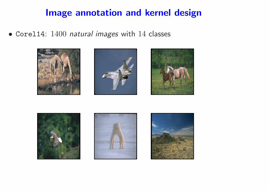
Image annotation and kernel design
• Corel14: 1400 natural images with 14 classes
Segmentation
• Goal: extract objects of interest
• Many methods available, ....
– ... but, rarely find the object of interest entirely
• Segmentation graphs
– Allows to work on “more reliable” over-segmentation
– Going to a large square grid (millions of pixels) to a small graph
(dozens or hundreds of regions)
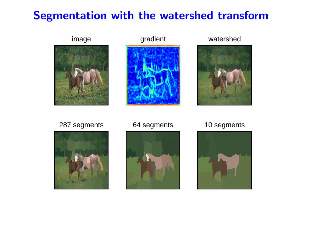
Segmentation with the watershed transform
image gradient watershed
287 segments 64 segments 10 segments
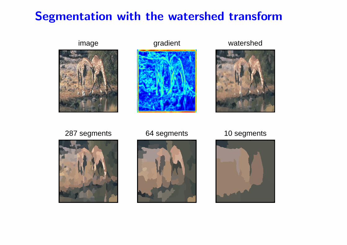
Segmentation with the watershed transform
image gradient watershed
287 segments 64 segments 10 segments
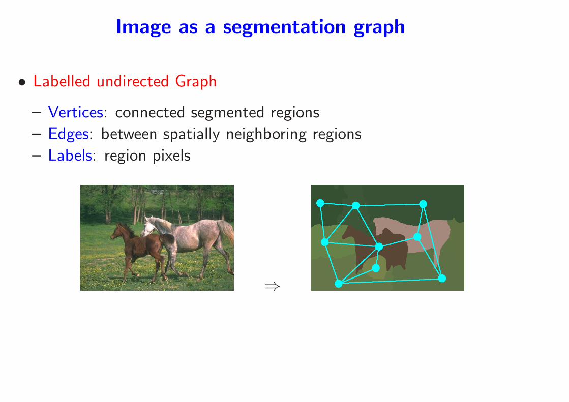
Image as a segmentation graph
• Labelled undirected Graph
– Vertices: connected segmented regions
– Edges: between spatially neighboring regions
– Labels: region pixels
⇒
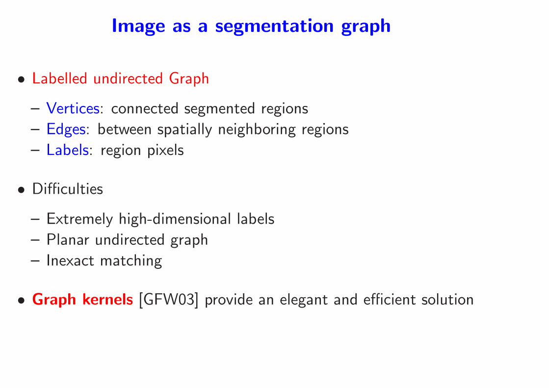
Image as a segmentation graph
• Labelled undirected Graph
– Vertices: connected segmented regions
– Edges: between spatially neighboring regions
– Labels: region pixels
• Difficulties
– Extremely high-dimensional labels
– Planar undirected graph
– Inexact matching
• Graph kernels [GFW03] provide an elegant and efficient solution

Kernels between structured objects
Strings, graphs, etc... [STC04]
• Numerous applications (text, bio-informatics)
• From probabilistic models on objects (e.g., Saunders et al, 2003)
• Enumeration of subparts (Haussler, 1998, Watkins, 1998)
– Efficient for strings
– Possibility of gaps, partial matches, very efficient algorithms
(Leslie et al, 2002, Lodhi et al, 2002, etc... )
• Most approaches fails for general graphs (even for undirected trees!)
– NP-Hardness results (Gartner et al, 2003)
– Need alternative set of subparts
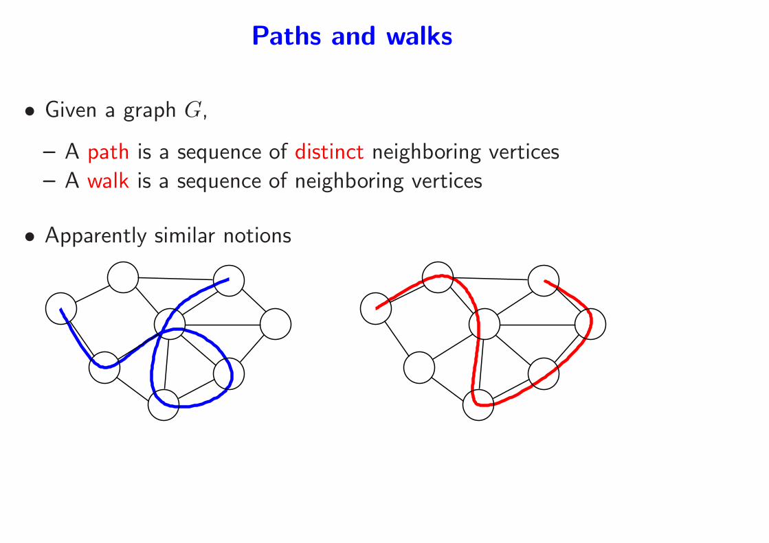
Paths and walks
• Given a graph G,
– A path is a sequence of distinct neighboring vertices
– A walk is a sequence of neighboring vertices
• Apparently similar notions
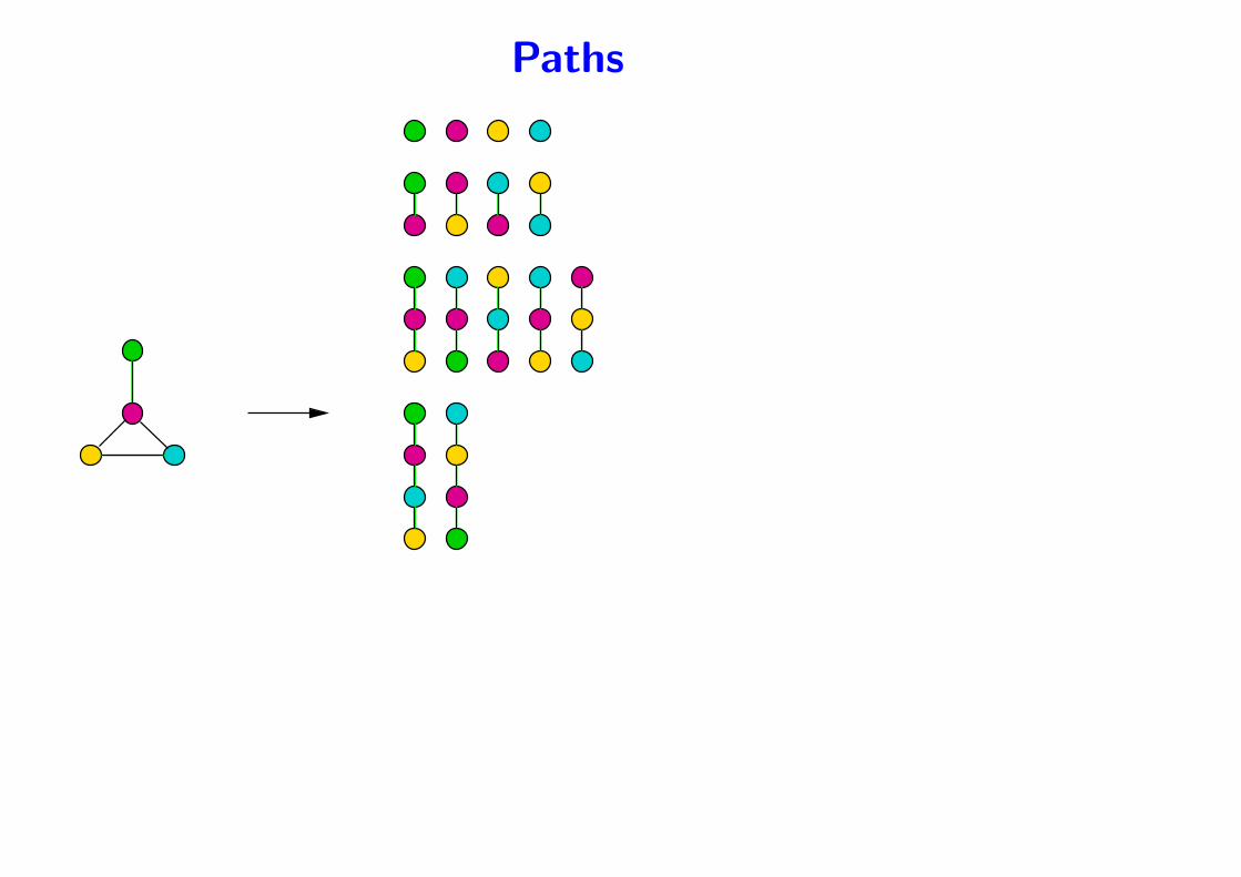
Paths
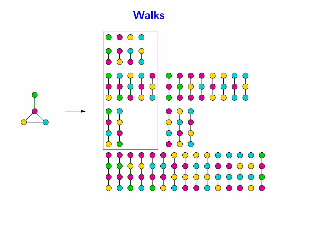
Walks
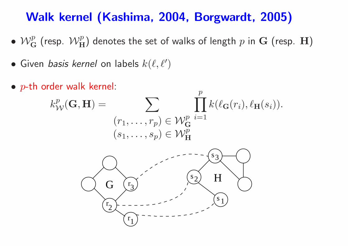
Walk kernel (Kashima, 2004, Borgwardt, 2005)
• WpG (resp. Wp
H) denotes the set of walks of length p in G (resp. H)
• Given basis kernel on labels k(ℓ, ℓ′)
• p-th order walk kernel:
kpW(G,H) =
∑
(r1, . . . , rp) ∈ WpG
(s1, . . . , sp) ∈ WpH
p∏
i=1
k(ℓG(ri), ℓH(si)).
G
1
s3
2s
s 1r2
3rH
r
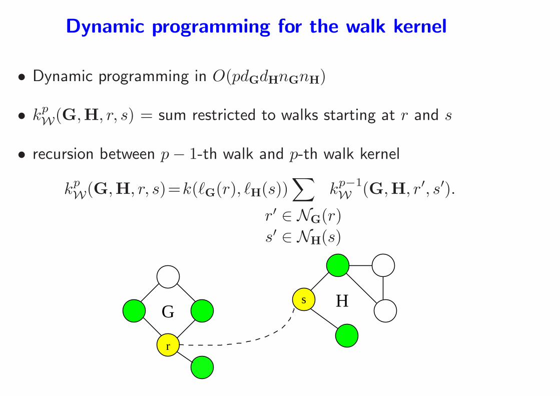
Dynamic programming for the walk kernel
• Dynamic programming in O(pdGdHnGnH)
• kpW(G,H, r, s) = sum restricted to walks starting at r and s
• recursion between p− 1-th walk and p-th walk kernel
kpW(G,H, r, s)=k(ℓG(r), ℓH(s))
∑
r′ ∈ NG(r)
s′ ∈ NH(s)
kp−1W (G,H, r′, s′).
Gs
r
H
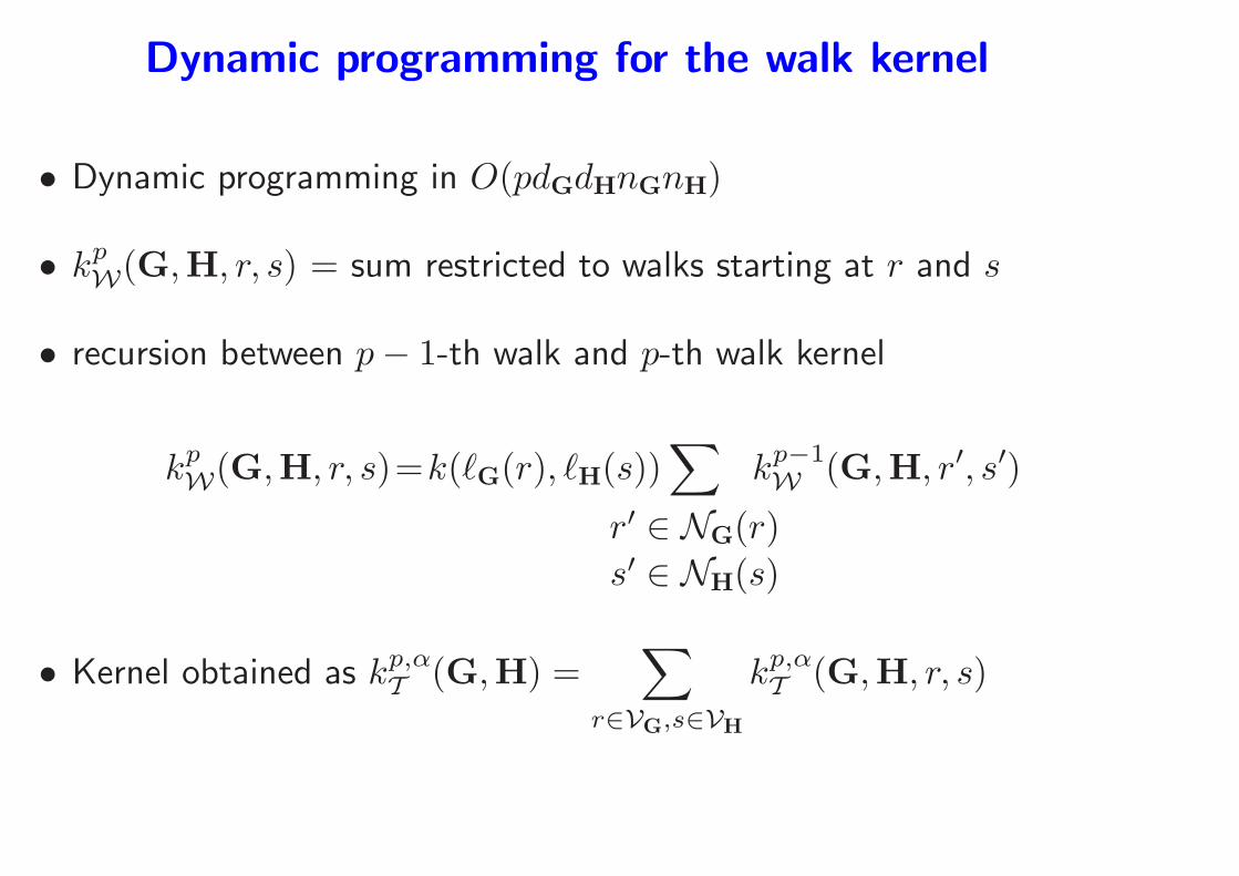
Dynamic programming for the walk kernel
• Dynamic programming in O(pdGdHnGnH)
• kpW(G,H, r, s) = sum restricted to walks starting at r and s
• recursion between p− 1-th walk and p-th walk kernel
kpW(G,H, r, s)=k(ℓG(r), ℓH(s))
∑
r′ ∈ NG(r)
s′ ∈ NH(s)
kp−1W (G,H, r′, s′)
• Kernel obtained as kp,αT (G,H) =
∑
r∈VG,s∈VH
kp,αT (G,H, r, s)
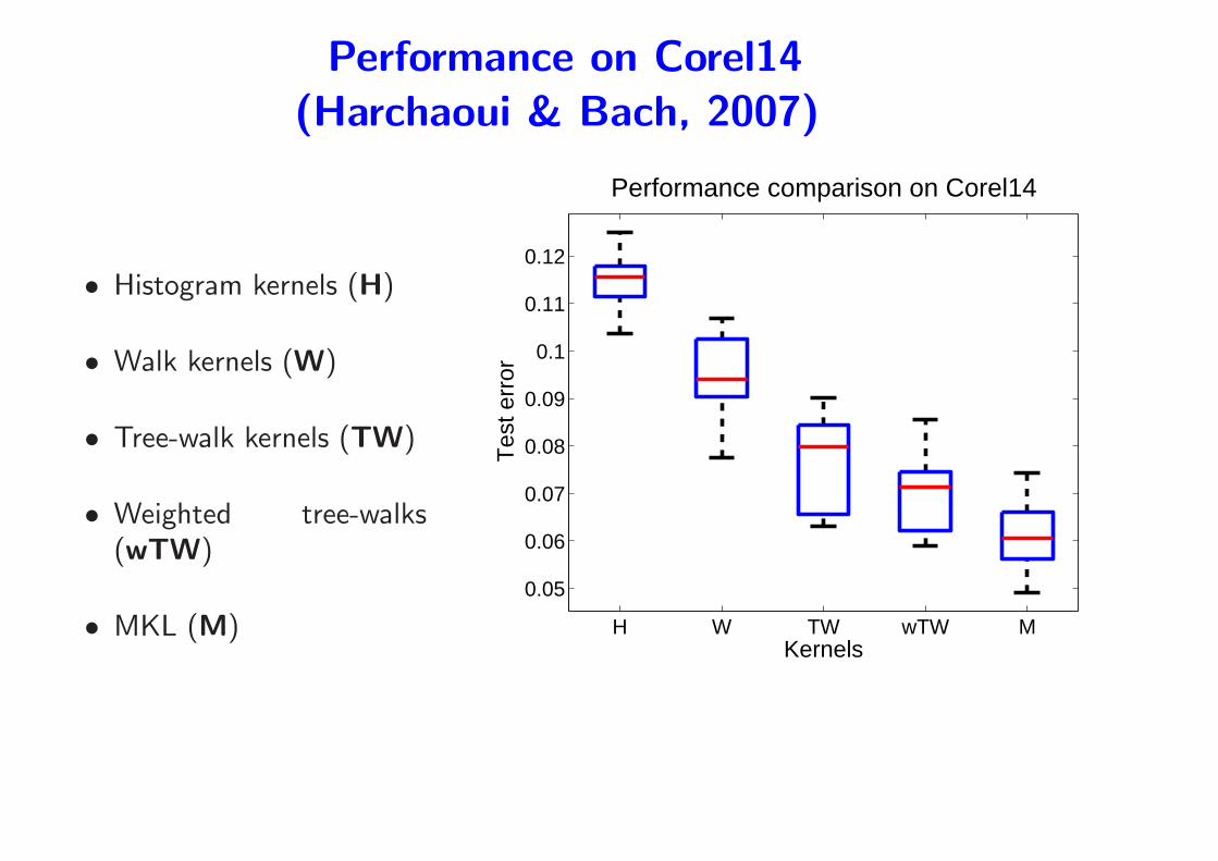
Performance on Corel14
(Harchaoui & Bach, 2007)
• Histogram kernels (H)
• Walk kernels (W)
• Tree-walk kernels (TW)
• Weighted tree-walks(wTW)
• MKL (M) H W TW wTW M
0.05
0.06
0.07
0.08
0.09
0.1
0.11
0.12
Tes
t err
or
Kernels
Performance comparison on Corel14
MKL
Summary
• Block ℓ1-norm extends regular ℓ1-norm
• One kernel per block
• Application:
– Data fusion
– Hyperparameter selection
– Non linear variable selection

Course Outline
1. ℓ1-norm regularization
• Review of nonsmooth optimization problems and algorithms
• Algorithms for the Lasso (generic or dedicated)
• Examples
2. Extensions
• Group Lasso and multiple kernel learning (MKL) + case study
• Sparse methods for matrices
• Sparse PCA
3. Theory - Consistency of pattern selection
• Low and high dimensional setting
• Links with compressed sensing
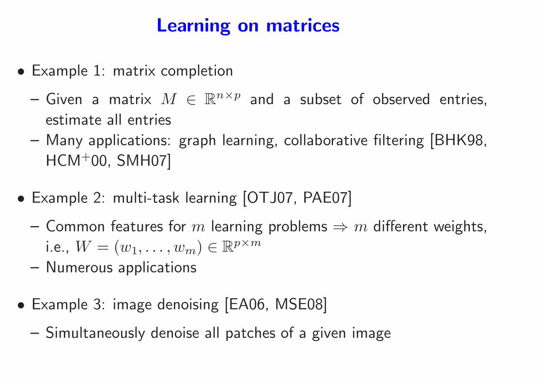
Learning on matrices
• Example 1: matrix completion
– Given a matrix M ∈ Rn×p and a subset of observed entries,
estimate all entries
– Many applications: graph learning, collaborative filtering [BHK98,
HCM+00, SMH07]
• Example 2: multi-task learning [OTJ07, PAE07]
– Common features for m learning problems ⇒ m different weights,
i.e., W = (w1, . . . , wm) ∈ Rp×m
– Numerous applications
• Example 3: image denoising [EA06, MSE08]
– Simultaneously denoise all patches of a given image
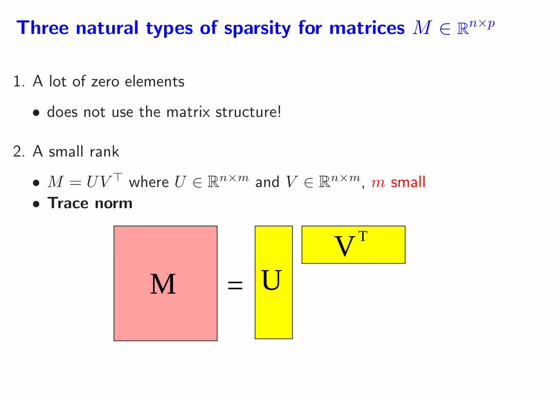
Three natural types of sparsity for matrices M ∈ Rn×p
1. A lot of zero elements
• does not use the matrix structure!
2. A small rank
• M = UV ⊤ where U ∈ Rn×m and V ∈ R
n×m, m small
• Trace norm
U=V
M
T
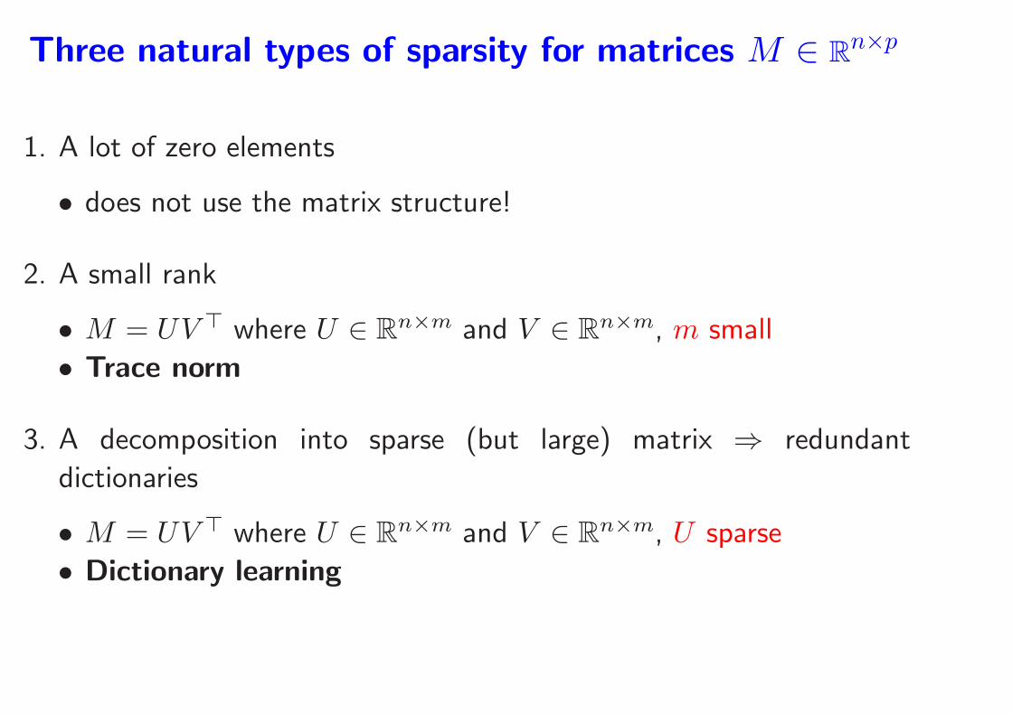
Three natural types of sparsity for matrices M ∈ Rn×p
1. A lot of zero elements
• does not use the matrix structure!
2. A small rank
• M = UV ⊤ where U ∈ Rn×m and V ∈ R
n×m, m small
• Trace norm
3. A decomposition into sparse (but large) matrix ⇒ redundant
dictionaries
• M = UV ⊤ where U ∈ Rn×m and V ∈ R
n×m, U sparse
• Dictionary learning
Trace norm [SRJ05, FHB01, Bac08c]
• Singular value decomposition: M ∈ Rn×p can always be decomposed
into M = U Diag(s)V ⊤, where U ∈ Rn×m and V ∈ R
n×m have
orthonormal columns and s is a positive vector (of singular values)
• ℓ0 norm of singular values = rank
• ℓ1 norm of singular values = trace norm
• Similar properties than the ℓ1-norm
– Convexity
– Solutions of penalized problem have low rank
– Algorithms
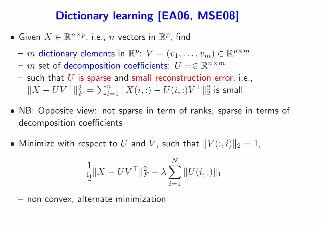
Dictionary learning [EA06, MSE08]
• Given X ∈ Rn×p, i.e., n vectors in R
p, find
– m dictionary elements in Rp: V = (v1, . . . , vm) ∈ R
p×m
– m set of decomposition coefficients: U =∈ Rn×m
– such that U is sparse and small reconstruction error, i.e.,
‖X − UV ⊤‖2F =∑n
i=1 ‖X(i, :)− U(i, :)V ⊤‖22 is small
• NB: Opposite view: not sparse in term of ranks, sparse in terms of
decomposition coefficients
• Minimize with respect to U and V , such that ‖V (:, i)‖2 = 1,
1
2‖X − UV ⊤‖2F + λ
N∑
i=1
‖U(i, :)‖1
– non convex, alternate minimization
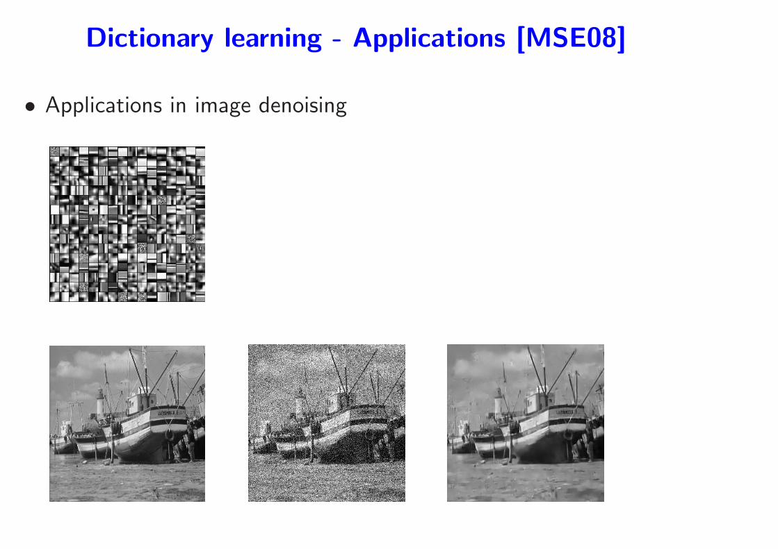
Dictionary learning - Applications [MSE08]
• Applications in image denoising
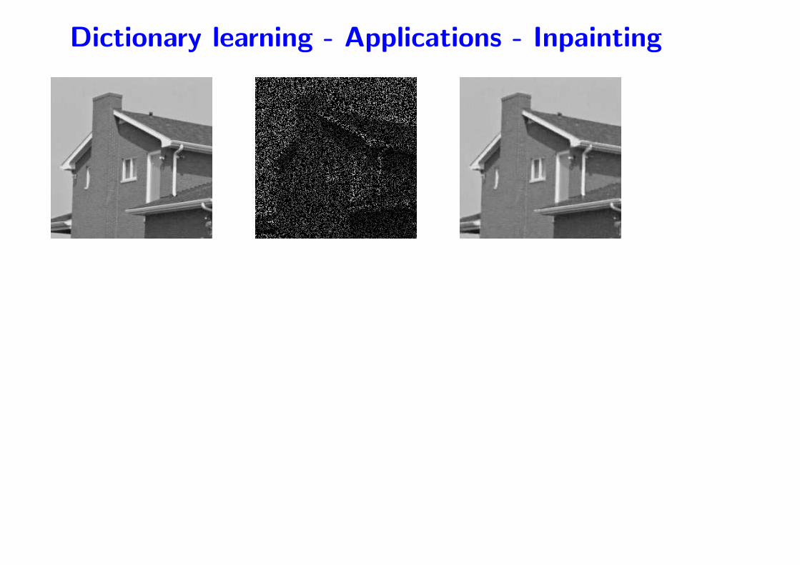
Dictionary learning - Applications - Inpainting
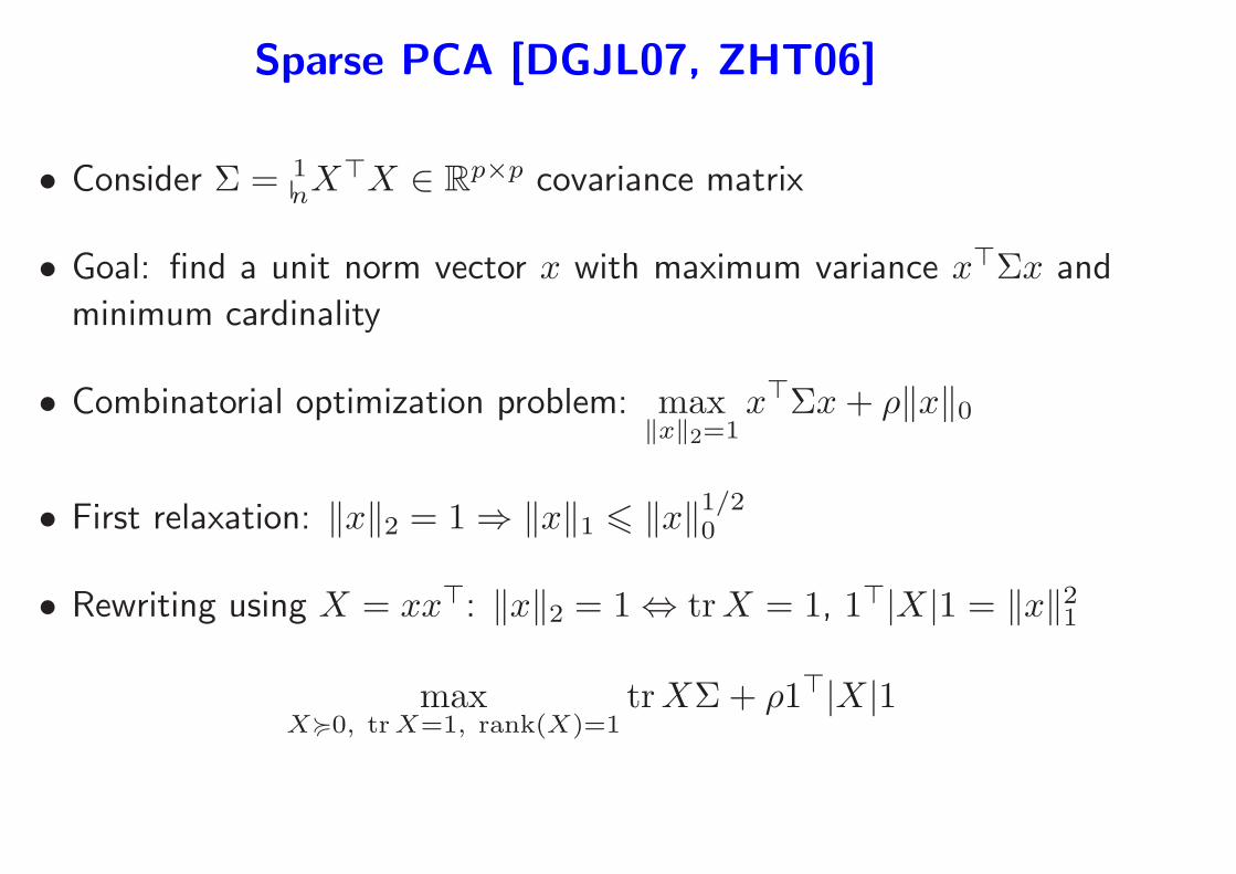
Sparse PCA [DGJL07, ZHT06]
• Consider Σ = 1nX
⊤X ∈ Rp×p covariance matrix
• Goal: find a unit norm vector x with maximum variance x⊤Σx and
minimum cardinality
• Combinatorial optimization problem: max‖x‖2=1
x⊤Σx+ ρ‖x‖0
• First relaxation: ‖x‖2 = 1⇒ ‖x‖1 6 ‖x‖1/20
• Rewriting using X = xx⊤: ‖x‖2 = 1⇔ trX = 1, 1⊤|X|1 = ‖x‖21
maxX<0, tr X=1, rank(X)=1
trXΣ + ρ1⊤|X|1
Sparse PCA [DGJL07, ZHT06]
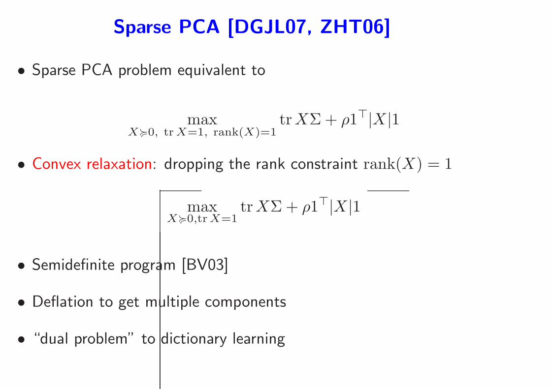
• Sparse PCA problem equivalent to
maxX<0, tr X=1, rank(X)=1
trXΣ + ρ1⊤|X|1
• Convex relaxation: dropping the rank constraint rank(X) = 1
maxX<0,tr X=1
trXΣ + ρ1⊤|X|1
• Semidefinite program [BV03]
• Deflation to get multiple components
• “dual problem” to dictionary learning
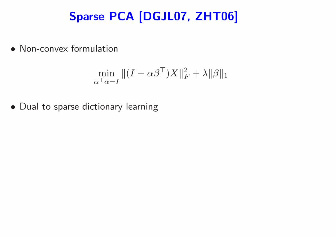
Sparse PCA [DGJL07, ZHT06]
• Non-convex formulation
minα⊤α=I
‖(I − αβ⊤)X‖2F + λ‖β‖1
• Dual to sparse dictionary learning

Sparse ???
•
Summary
• Notion of sparsity quite general
• Interesting links with convexity
– Convex relaxation
• Sparsifying the world
– All linear methods can be kernelized
– All linear methods can be sparsified
∗ Sparse PCA
∗ Sparse LDA
∗ Sparse ....
Course Outline
1. ℓ1-norm regularization
• Review of nonsmooth optimization problems and algorithms
• Algorithms for the Lasso (generic or dedicated)
• Examples
2. Extensions
• Group Lasso and multiple kernel learning (MKL) + case study
• Sparse methods for matrices
• Sparse PCA
3. Theory - Consistency of pattern selection
• Low and high dimensional setting
• Links with compressed sensing
Theory
• Sparsity-inducing norms often used heuristically
• When does it converge to the correct pattern?
– Yes if certain conditions on the problem are satisfied (low
correlation)
– what if not?
• Links with compressed sensing
Model consistency of the Lasso
• Sparsity-inducing norms often used heuristically
• If the responses y1, . . . , yn are such that yi = w⊤0 xi + εi where εi are
i.i.d. and w0 is sparse, do we get back the correct pattern of zeros?
• Intuitive answer: yes if and ony if some consistency condition on
the generating covariance matrices is satisfied [ZY06, YL07, Zou06,
Wai06]
Asymptotic analysis - Low dimensional setting
• Asymptotic set up
– data generated from linear model Y = X⊤w + ε
– w any minimizer of the Lasso problem
– number of observations n tends to infinity
• Three types of consistency
– regular consistency: ‖w −w‖2 tends to zero in probability
– pattern consistency: the sparsity pattern J = {j, wj 6= 0} tends
to J = {j, wj 6= 0} in probability
– sign consistency: the sign vector s = sign(w) tends to s = sign(w)
in probability
• NB: with our assumptions, pattern and sign consistencies are
equivalent once we have regular consistency
Assumptions for analysis
• Simplest assumptions (fixed p, large n):
1. Sparse linear model: Y = X⊤w + ε , ε independent from X, and
w sparse.
2. Finite cumulant generating functions E exp(a‖X‖22) and
E exp(aε2) finite for some a > 0 (e.g., Gaussian noise)
3. Invertible matrix of second order moments Q = E(XX⊤) ∈ Rp×p.
Asymptotic analysis - simple cases
minw∈Rp12n‖Y −Xw‖22 + µn‖w‖1
• If µn tends to infinity
– w tends to zero with probability tending to one
– J tends to ∅ in probability
Asymptotic analysis - simple cases
minw∈Rp12n‖y −Xw‖22 + µn‖w‖1
• If µn tends to infinity
– w tends to zero with probability tending to one
– J tends to ∅ in probability
• If µn tends to µ0 ∈ (0,∞)
– w converges to the minimum of 12(w −w)⊤Q(w −w) + µ0‖w‖1
– The sparsity and sign patterns may or may not be consistent
– Possible to have sign consistency without regular consistency
Asymptotic analysis - simple cases
minw∈Rp12n‖Y −Xw‖22 + µn‖w‖1
• If µn tends to infinity
– w tends to zero with probability tending to one
– J tends to ∅ in probability
• If µn tends to µ0 ∈ (0,∞)
– w converges to the minimum of 12(w −w)⊤Q(w −w) + µ0‖w‖1
– The sparsity and sign patterns may or may not be consistent
– Possible to have sign consistency without regular consistency
• If µn tends to zero faster than n−1/2
– w converges in probability to w
– With probability tending to one, all variables are included
Asymptotic analysis - important case
minw∈Rp12n‖Y −Xw‖22 + µn‖w‖1
• If µn tends to zero slower than n−1/2
– w converges in probability to w
– the sign pattern converges to the one of the minimum of
12v
⊤Qv + v⊤J sign(wJ) + ‖vJc‖1
– The sign pattern is equal to s (i.e., sign consistency) if and only if
‖QJcJQ−1JJ sign(wJ)‖∞ 6 1
– Consistency condition found by many authors: Yuan & Lin (2007),
Wainwright (2006), Zhao & Yu (2007), Zou (2006)
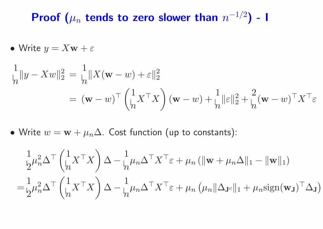
Proof (µn tends to zero slower than n−1/2) - I
• Write y = Xw + ε
1
n‖y −Xw‖22 =
1
n‖X(w − w) + ε‖22
= (w − w)⊤(
1
nX⊤X
)
(w − w) +1
n‖ε‖22 +
2
n(w − w)⊤X⊤ε
• Write w = w + µn∆. Cost function (up to constants):
1
2µ2
n∆⊤
(
1
nX⊤X
)
∆− 1
nµn∆⊤X⊤ε+ µn (‖w + µn∆‖1 − ‖w‖1)
=1
2µ2
n∆⊤
(
1
nX⊤X
)
∆− 1
nµn∆⊤X⊤ε+ µn
(
µn‖∆Jc‖1 + µnsign(wJ)⊤∆J
)
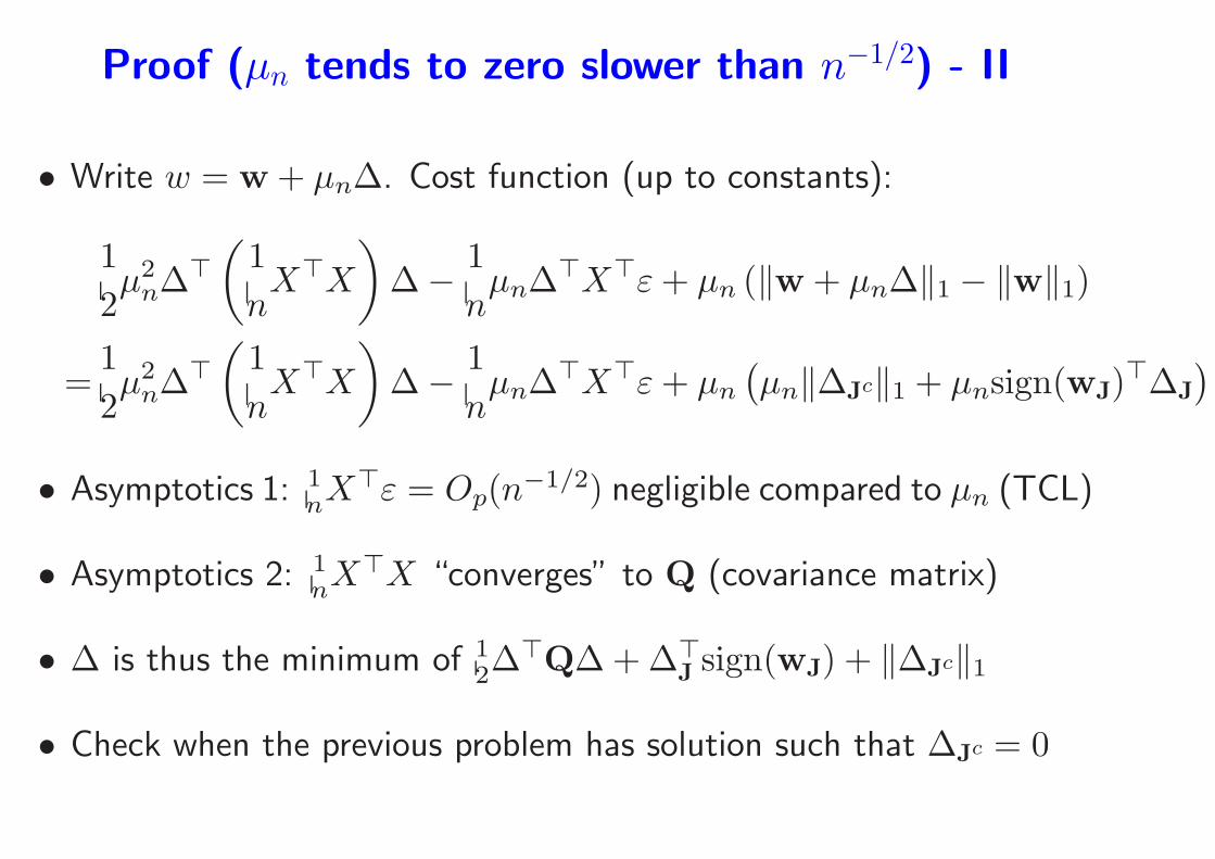
Proof (µn tends to zero slower than n−1/2) - II
• Write w = w + µn∆. Cost function (up to constants):
1
2µ2
n∆⊤
(
1
nX⊤X
)
∆− 1
nµn∆⊤X⊤ε+ µn (‖w + µn∆‖1 − ‖w‖1)
=1
2µ2
n∆⊤
(
1
nX⊤X
)
∆− 1
nµn∆⊤X⊤ε+ µn
(
µn‖∆Jc‖1 + µnsign(wJ)⊤∆J
)
• Asymptotics 1: 1nX
⊤ε = Op(n−1/2) negligible compared to µn (TCL)
• Asymptotics 2: 1nX
⊤X “converges” to Q (covariance matrix)
• ∆ is thus the minimum of 12∆
⊤Q∆ + ∆⊤J sign(wJ) + ‖∆Jc‖1
• Check when the previous problem has solution such that ∆Jc = 0
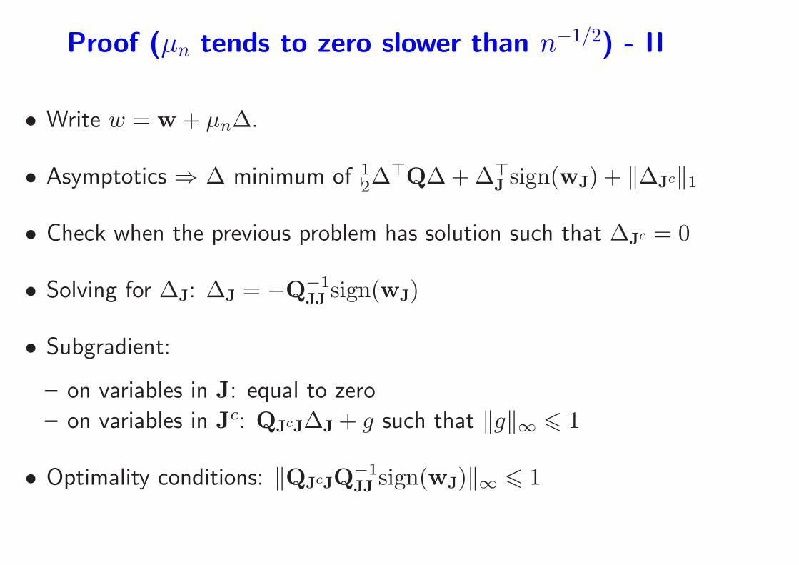
Proof (µn tends to zero slower than n−1/2) - II
• Write w = w + µn∆.
• Asymptotics ⇒ ∆ minimum of 12∆
⊤Q∆ + ∆⊤J sign(wJ) + ‖∆Jc‖1
• Check when the previous problem has solution such that ∆Jc = 0
• Solving for ∆J: ∆J = −Q−1JJ sign(wJ)
• Subgradient:
– on variables in J: equal to zero
– on variables in Jc: QJcJ∆J + g such that ‖g‖∞ 6 1
• Optimality conditions: ‖QJcJQ−1JJ sign(wJ)‖∞ 6 1
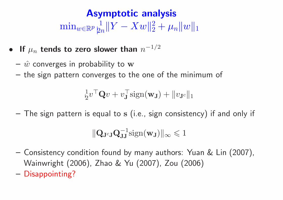
Asymptotic analysis
minw∈Rp12n‖Y −Xw‖22 + µn‖w‖1
• If µn tends to zero slower than n−1/2
– w converges in probability to w
– the sign pattern converges to the one of the minimum of
12v
⊤Qv + v⊤J sign(wJ) + ‖vJc‖1
– The sign pattern is equal to s (i.e., sign consistency) if and only if
‖QJcJQ−1JJ sign(wJ)‖∞ 6 1
– Consistency condition found by many authors: Yuan & Lin (2007),
Wainwright (2006), Zhao & Yu (2007), Zou (2006)
– Disappointing?
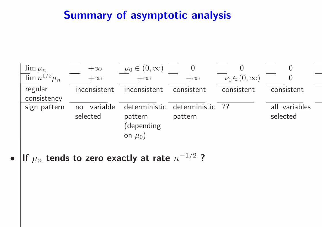
Summary of asymptotic analysis
limµn +∞ µ0 ∈ (0,∞) 0 0 0limn1/2µn +∞ +∞ +∞ ν0∈(0,∞) 0
regularconsistency
inconsistent inconsistent consistent consistent consistent
sign pattern no variableselected
deterministicpattern(dependingon µ0)
deterministicpattern
?? all variablesselected
• If µn tends to zero exactly at rate n−1/2 ?
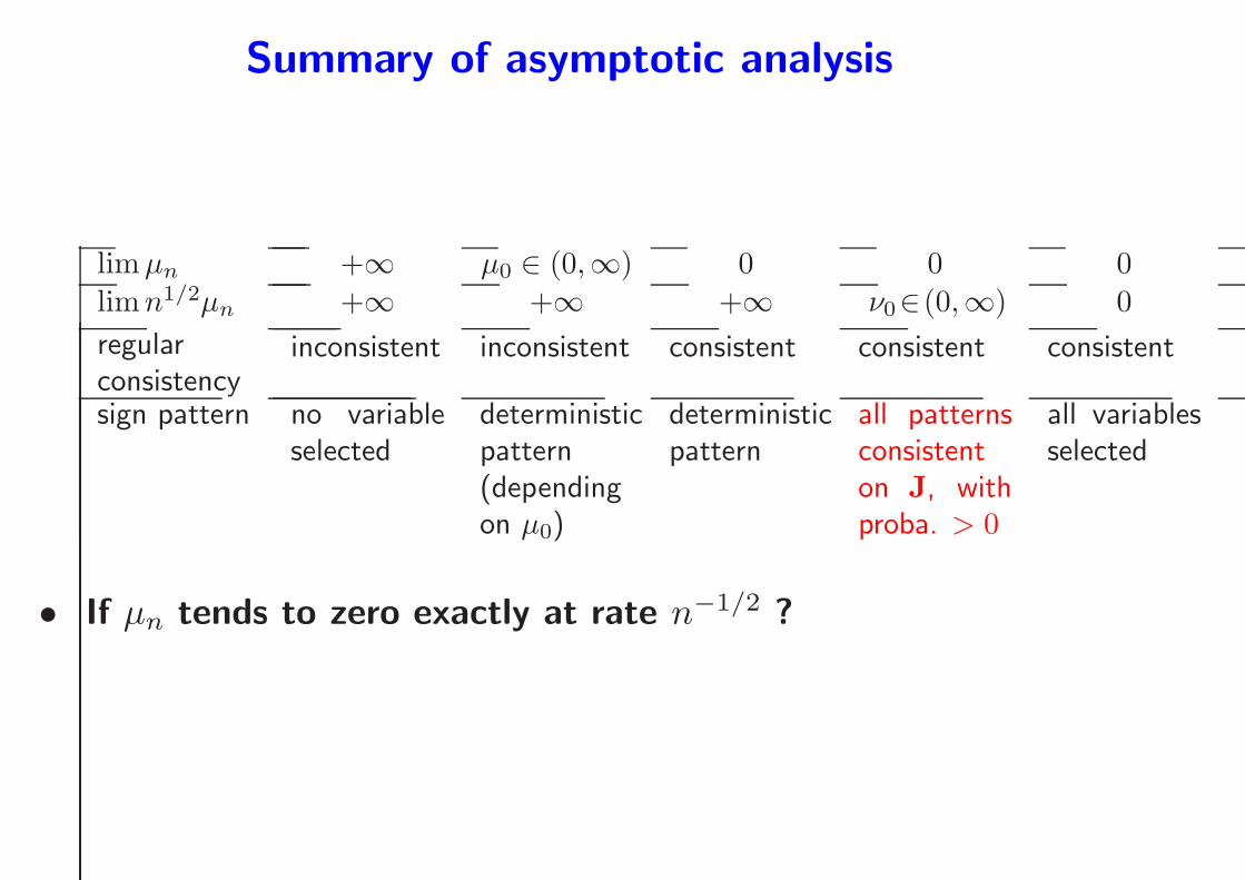
Summary of asymptotic analysis
limµn +∞ µ0 ∈ (0,∞) 0 0 0limn1/2µn +∞ +∞ +∞ ν0∈(0,∞) 0
regularconsistency
inconsistent inconsistent consistent consistent consistent
sign pattern no variableselected
deterministicpattern(dependingon µ0)
deterministicpattern
all patternsconsistenton J, withproba. > 0
all variablesselected
• If µn tends to zero exactly at rate n−1/2 ?
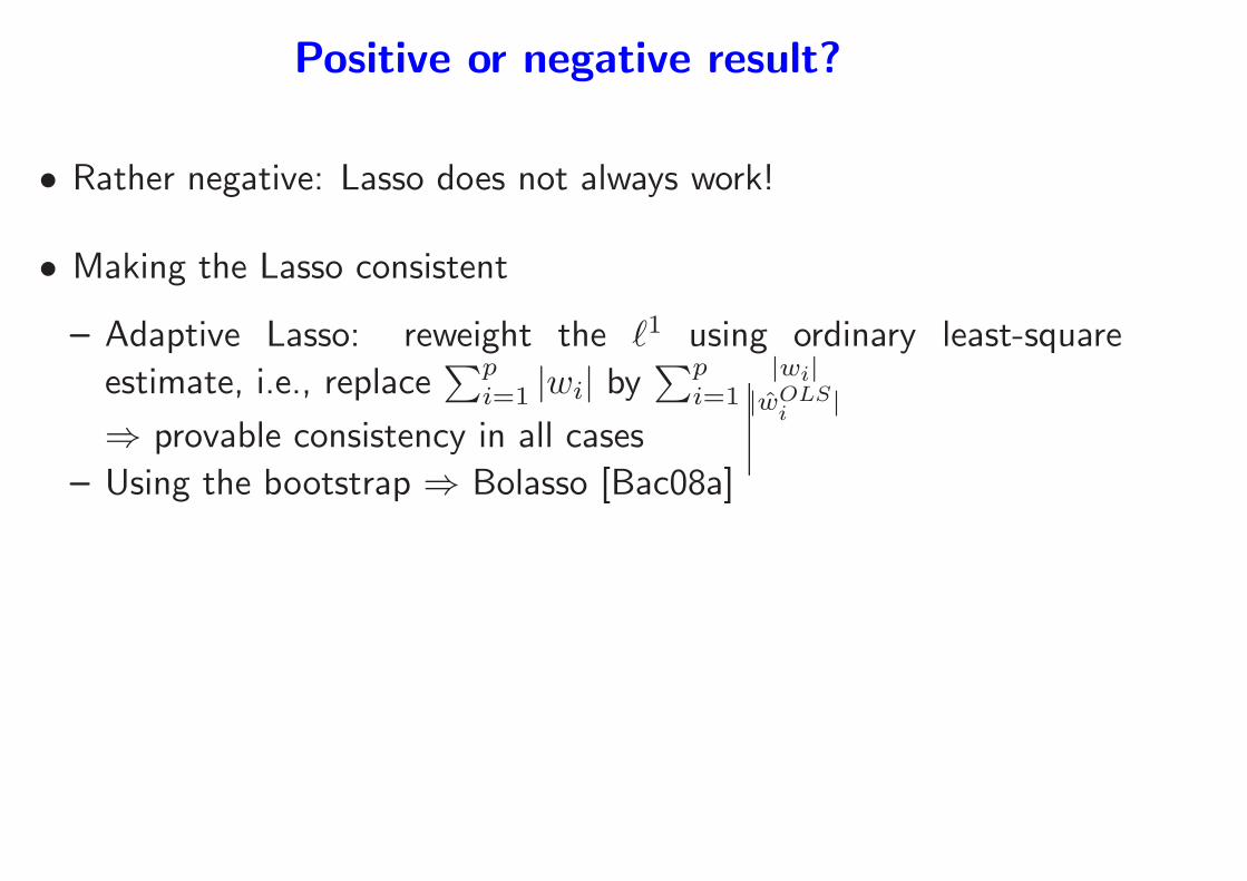
Positive or negative result?
• Rather negative: Lasso does not always work!
• Making the Lasso consistent
– Adaptive Lasso: reweight the ℓ1 using ordinary least-square
estimate, i.e., replace∑p
i=1 |wi| by∑p
i=1|wi|
|wOLSi |
⇒ provable consistency in all cases
– Using the bootstrap ⇒ Bolasso [Bac08a]
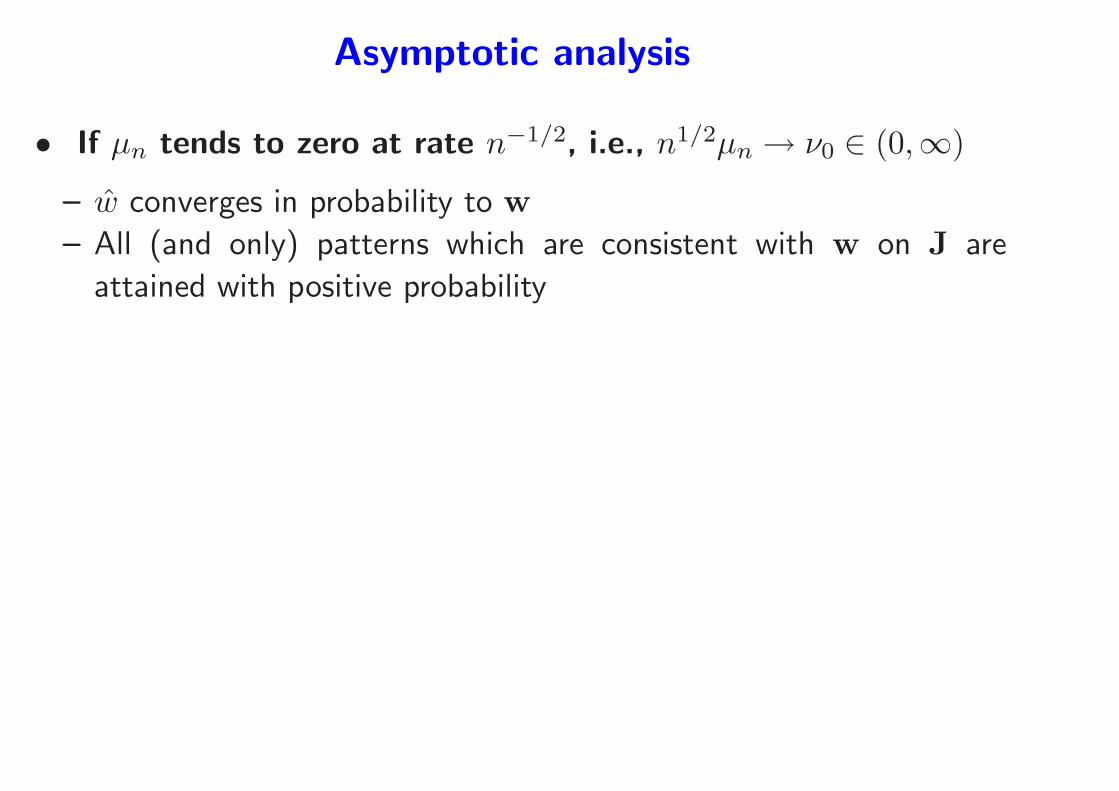
Asymptotic analysis
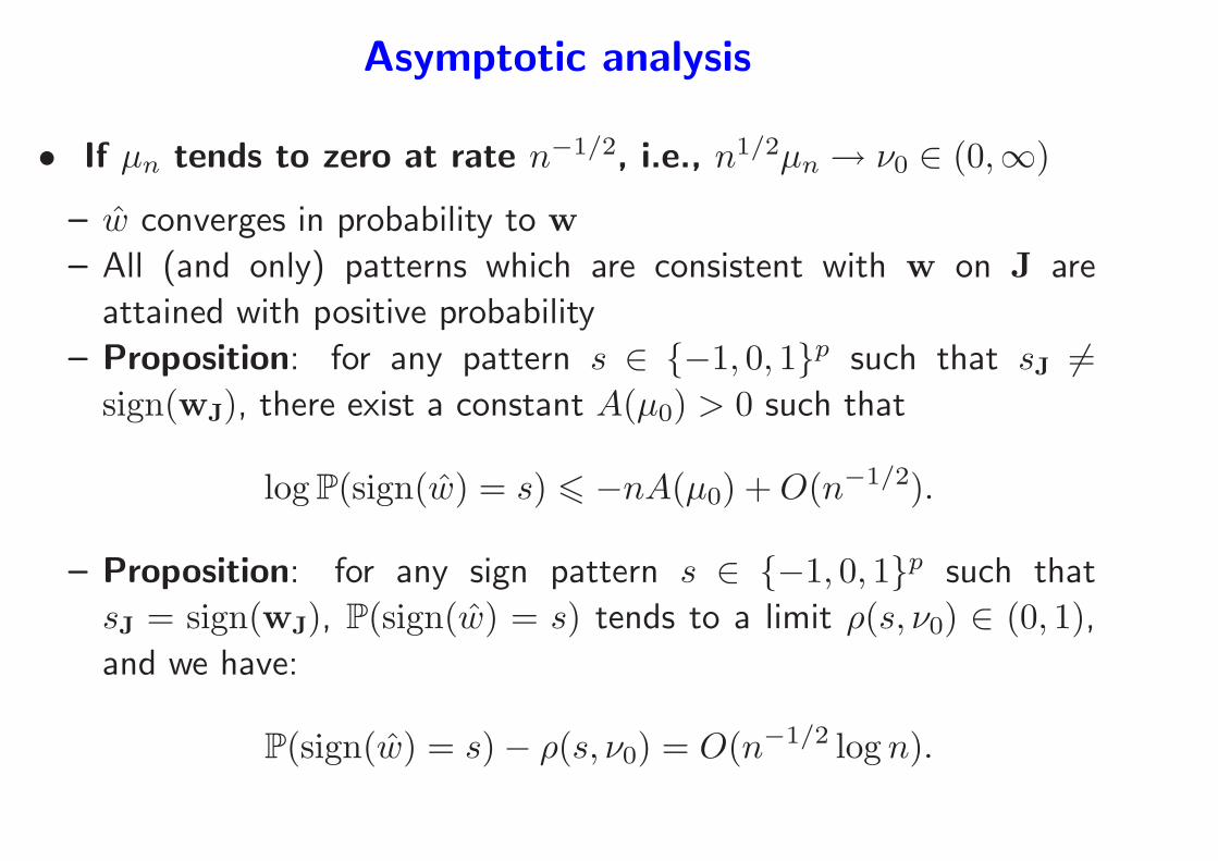
• If µn tends to zero at rate n−1/2, i.e., n1/2µn → ν0 ∈ (0,∞)
– w converges in probability to w
– All (and only) patterns which are consistent with w on J are
attained with positive probability
Asymptotic analysis
• If µn tends to zero at rate n−1/2, i.e., n1/2µn → ν0 ∈ (0,∞)
– w converges in probability to w
– All (and only) patterns which are consistent with w on J are
attained with positive probability
– Proposition: for any pattern s ∈ {−1, 0, 1}p such that sJ 6=sign(wJ), there exist a constant A(µ0) > 0 such that
log P(sign(w) = s) 6 −nA(µ0) +O(n−1/2).
– Proposition: for any sign pattern s ∈ {−1, 0, 1}p such that
sJ = sign(wJ), P(sign(w) = s) tends to a limit ρ(s, ν0) ∈ (0, 1),
and we have:
P(sign(w) = s)− ρ(s, ν0) = O(n−1/2 log n).
µn tends to zero at rate n−1/2
• Summary of asymptotic behavior:
– All relevant variables (i.e., the ones in J) are selected with
probability tending to one exponentially fast
– All other variables are selected with strictly positive probability
µn tends to zero at rate n−1/2
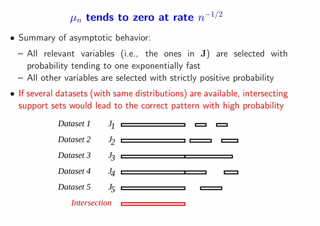
• Summary of asymptotic behavior:
– All relevant variables (i.e., the ones in J) are selected with
probability tending to one exponentially fast
– All other variables are selected with strictly positive probability
• If several datasets (with same distributions) are available, intersecting
support sets would lead to the correct pattern with high probability
Dataset 1
2
1J
Intersection
5
4
3
JDataset 5
J
JDataset 3
Dataset 4
Dataset 2 J
Bootstrap
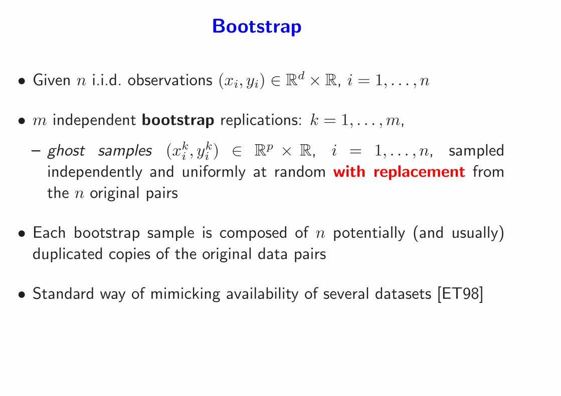
• Given n i.i.d. observations (xi, yi) ∈ Rd × R, i = 1, . . . , n
• m independent bootstrap replications: k = 1, . . . ,m,
– ghost samples (xki , y
ki ) ∈ R
p × R, i = 1, . . . , n, sampled
independently and uniformly at random with replacement from
the n original pairs
• Each bootstrap sample is composed of n potentially (and usually)
duplicated copies of the original data pairs
• Standard way of mimicking availability of several datasets [ET98]
Bolasso algorithm
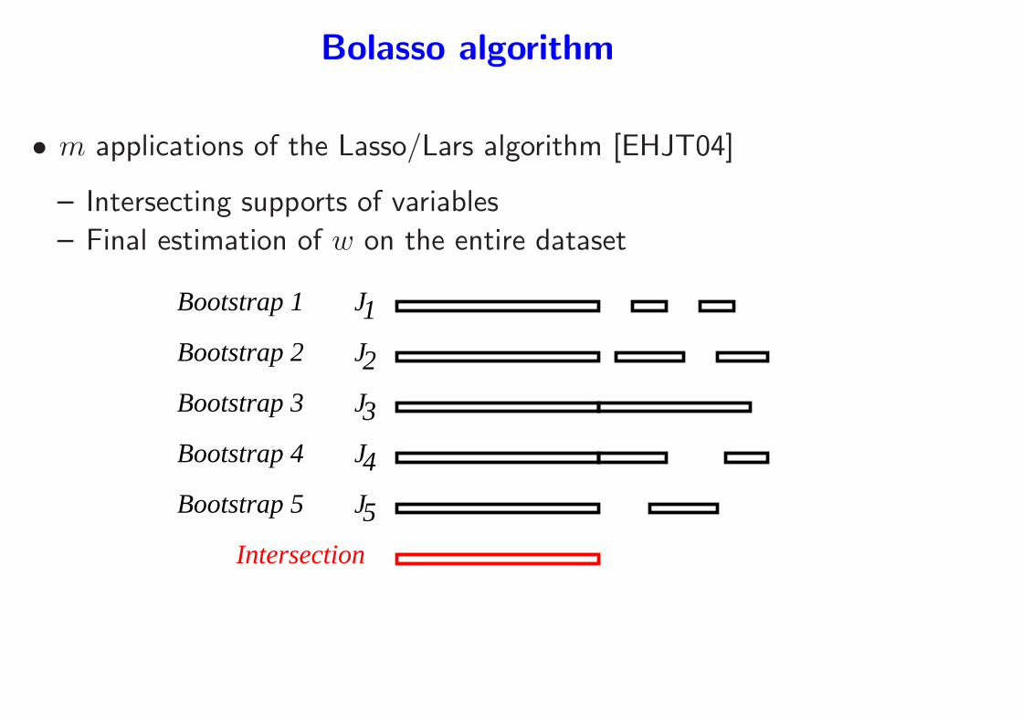
• m applications of the Lasso/Lars algorithm [EHJT04]
– Intersecting supports of variables
– Final estimation of w on the entire dataset
J
2
1J
Bootstrap 4
Bootstrap 5
Bootstrap 2
Bootstrap 3
Bootstrap 1
Intersection
5
4
3
J
J
J
Bolasso - Consistency result
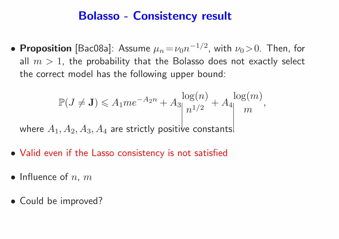
• Proposition [Bac08a]: Assume µn=ν0n−1/2, with ν0>0. Then, for
all m > 1, the probability that the Bolasso does not exactly select
the correct model has the following upper bound:
P(J 6= J) 6 A1me−A2n +A3
log(n)
n1/2+A4
log(m)
m,
where A1, A2, A3, A4 are strictly positive constants.
• Valid even if the Lasso consistency is not satisfied
• Influence of n, m
• Could be improved?
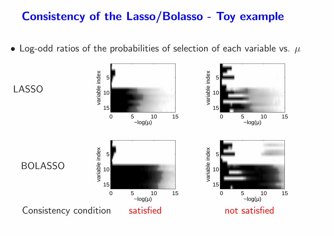
Consistency of the Lasso/Bolasso - Toy example
• Log-odd ratios of the probabilities of selection of each variable vs. µ
LASSO
−log(µ)
varia
ble
inde
x
0 5 10 15
5
10
15
−log(µ)
varia
ble
inde
x
0 5 10 15
5
10
15
BOLASSO
−log(µ)
varia
ble
inde
x
0 5 10 15
5
10
15
−log(µ)
varia
ble
inde
x
0 5 10 15
5
10
15
Consistency condition satisfied not satisfied
High-dimensional setting
• p > n: important case with harder analysis (no invertible covariance
matrices)
• If consistency condition is satisfied, the Lasso is indeed consistent as
long as log(p) << n
• A lot of on-going work [MY08, Wai06]
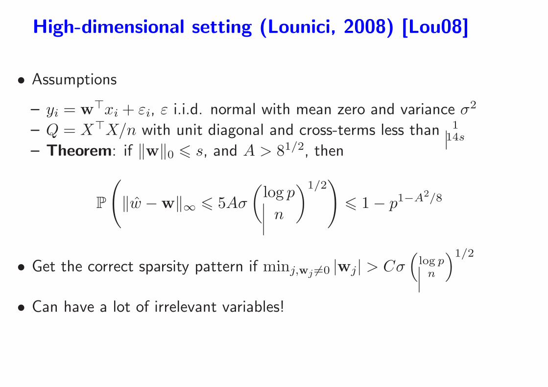
High-dimensional setting (Lounici, 2008) [Lou08]
• Assumptions
– yi = w⊤xi + εi, ε i.i.d. normal with mean zero and variance σ2
– Q = X⊤X/n with unit diagonal and cross-terms less than 114s
– Theorem: if ‖w‖0 6 s, and A > 81/2, then
P
(
‖w −w‖∞ 6 5Aσ
(
log p
n
)1/2)
6 1− p1−A2/8
• Get the correct sparsity pattern if minj,wj 6=0 |wj| > Cσ(
log pn
)1/2
• Can have a lot of irrelevant variables!
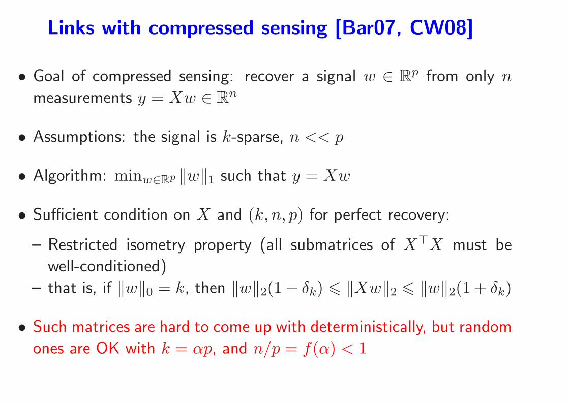
Links with compressed sensing [Bar07, CW08]
• Goal of compressed sensing: recover a signal w ∈ Rp from only n
measurements y = Xw ∈ Rn
• Assumptions: the signal is k-sparse, n << p
• Algorithm: minw∈Rp ‖w‖1 such that y = Xw
• Sufficient condition on X and (k, n, p) for perfect recovery:
– Restricted isometry property (all submatrices of X⊤X must be
well-conditioned)
– that is, if ‖w‖0 = k, then ‖w‖2(1− δk) 6 ‖Xw‖2 6 ‖w‖2(1 + δk)
• Such matrices are hard to come up with deterministically, but random
ones are OK with k = αp, and n/p = f(α) < 1

Course Outline
1. ℓ1-norm regularization
• Review of nonsmooth optimization problems and algorithms
• Algorithms for the Lasso (generic or dedicated)
• Examples
2. Extensions
• Group Lasso and multiple kernel learning (MKL) + case study
• Sparse methods for matrices
• Sparse PCA
3. Theory - Consistency of pattern selection
• Low and high dimensional setting
• Links with compressed sensing
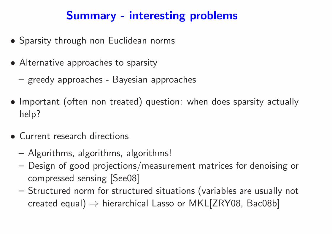
Summary - interesting problems
• Sparsity through non Euclidean norms
• Alternative approaches to sparsity
– greedy approaches - Bayesian approaches
• Important (often non treated) question: when does sparsity actually
help?
• Current research directions
– Algorithms, algorithms, algorithms!
– Design of good projections/measurement matrices for denoising or
compressed sensing [See08]
– Structured norm for structured situations (variables are usually not
created equal) ⇒ hierarchical Lasso or MKL[ZRY08, Bac08b]

Lasso in action
2 3 4 5 6 70
0.1
0.2
0.3
0.4
0.5
0.6
0.7
0.8
0.9
1
log2(p)
test
set
err
or
2 3 4 5 6 70
0.1
0.2
0.3
0.4
0.5
0.6
0.7
0.8
0.9
1
log2(p)
test
set
err
or
L1greedyL2
L1greedyL2
(left: sparsity is expected, right: sparsity is not expected)
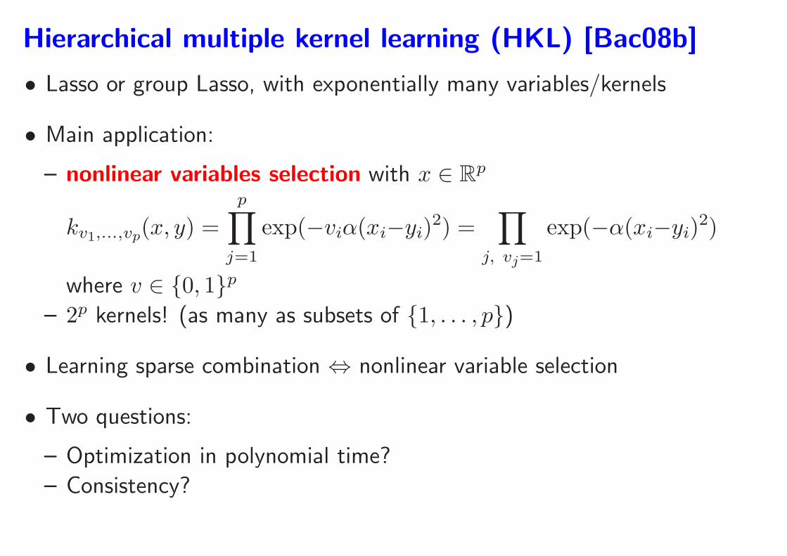
Hierarchical multiple kernel learning (HKL) [Bac08b]
• Lasso or group Lasso, with exponentially many variables/kernels
• Main application:
– nonlinear variables selection with x ∈ Rp
kv1,...,vp(x, y) =
p∏
j=1
exp(−viα(xi−yi)2) =
∏
j, vj=1
exp(−α(xi−yi)2)
where v ∈ {0, 1}p– 2p kernels! (as many as subsets of {1, . . . , p})
• Learning sparse combination ⇔ nonlinear variable selection
• Two questions:
– Optimization in polynomial time?
– Consistency?
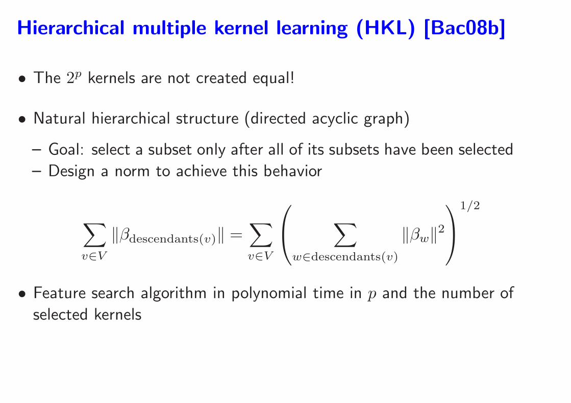
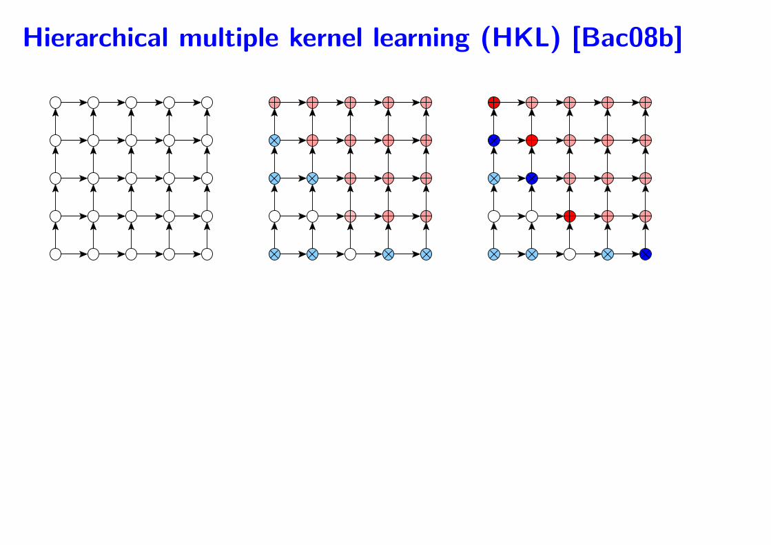
Hierarchical multiple kernel learning (HKL) [Bac08b]
• The 2p kernels are not created equal!
• Natural hierarchical structure (directed acyclic graph)
– Goal: select a subset only after all of its subsets have been selected
– Design a norm to achieve this behavior
∑
v∈V
‖βdescendants(v)‖ =∑
v∈V
∑
w∈descendants(v)
‖βw‖2
1/2
• Feature search algorithm in polynomial time in p and the number of
selected kernels
Hierarchical multiple kernel learning (HKL) [Bac08b]
References
[Aro50] N. Aronszajn. Theory of reproducing kernels. Trans. Am. Math. Soc., 68:337–404, 1950.
[Bac08a] F. Bach. Bolasso: model consistent lasso estimation through the bootstrap. In Proceedings
of the Twenty-fifth International Conference on Machine Learning (ICML), 2008.
[Bac08b] F. Bach. Exploring large feature spaces with hierarchical multiple kernel learning. In Adv.
NIPS, 2008.
[Bac08c] F. R. Bach. Consistency of trace norm minimization. Journal of Machine Learning
Research, to appear, 2008.
[Bar07] Richard Baraniuk. Compressive sensing. IEEE Signal Processing Magazine, 24(4):118–121,
2007.
[BB08] Leon Bottou and Olivier Bousquet. Learning using large datasets. In Mining Massive
DataSets for Security, NATO ASI Workshop Series. IOS Press, Amsterdam, 2008. to
appear.
[BGLS03] J. F. Bonnans, J. C. Gilbert, C. Lemarechal, and C. A. Sagastizbal. Numerical Optimization
Theoretical and Practical Aspects. Springer, 2003.
[BHH06] F. R. Bach, D. Heckerman, and E. Horvitz. Considering cost asymmetry in learning
classifiers. Journal of Machine Learning Research, 7:1713–1741, 2006.
[BHK98] J. S. Breese, D. Heckerman, and C. Kadie. Empirical analysis of predictive algorithms for
collaborative filtering. In 14th Conference on Uncertainty in Artificial Intelligence, pages
43–52, Madison, W.I., 1998. Morgan Kaufman.

[BL00] J. M. Borwein and A. S. Lewis. Convex Analysis and Nonlinear Optimization. Number 3
in CMS Books in Mathematics. Springer-Verlag, 2000.
[BLJ04] F. R. Bach, G. R. G. Lanckriet, and M. I. Jordan. Multiple kernel learning, conic duality,
and the SMO algorithm. In Proceedings of the International Conference on Machine
Learning (ICML), 2004.
[BTJ04] F. R. Bach, R. Thibaux, and M. I. Jordan. Computing regularization paths for learning
multiple kernels. In Advances in Neural Information Processing Systems 17, 2004.
[BV03] S. Boyd and L. Vandenberghe. Convex Optimization. Cambridge Univ. Press, 2003.
[CDS01] Scott Shaobing Chen, David L. Donoho, and Michael A. Saunders. Atomic decomposition
by basis pursuit. SIAM Rev., 43(1):129–159, 2001.
[CW08] Emmanuel Candes and Michael Wakin. An introduction to compressive sampling. IEEE
Signal Processing Magazine, 25(2):21–30, 2008.
[DGJL07] A. D’aspremont, El L. Ghaoui, M. I. Jordan, and G. R. G. Lanckriet. A direct formulation
for sparse PCA using semidefinite programming. SIAM Review, 49(3):434–48, 2007.
[EA06] M. Elad and M. Aharon. Image denoising via sparse and redundant representations over
learned dictionaries. IEEE Trans. Image Proc., 15(12):3736–3745, 2006.
[EHJT04] B. Efron, T. Hastie, I. Johnstone, and R. Tibshirani. Least angle regression. Ann. Stat.,
32:407, 2004.
[ET98] B. Efron and R. J. Tibshirani. An Introduction to the Bootstrap. Chapman & Hall, 1998.
[FHB01] M. Fazel, H. Hindi, and S. P. Boyd. A rank minimization heuristic with application
to minimum order system approximation. In Proceedings American Control Conference,
volume 6, pages 4734–4739, 2001.
[GFW03] Thomas Gartner, Peter A. Flach, and Stefan Wrobel. On graph kernels: Hardness results
and efficient alternatives. In COLT, 2003.
[HB07] Z. Harchaoui and F. R. Bach. Image classification with segmentation graph kernels. In
Proceedings of the Conference on Computer Vision and Pattern Recognition (CVPR),
2007.
[HCM+00] D. Heckerman, D. M. Chickering, C. Meek, R. Rounthwaite, and C. Kadie. Dependency
networks for inference, collaborative filtering, and data visualization. J. Mach. Learn. Res.,
1:49–75, 2000.
[HRTZ05] T. Hastie, S. Rosset, R. Tibshirani, and J. Zhu. The entire regularization path for the
support vector machine. Journal of Machine Learning Research, 5:1391–1415, 2005.
[HTF01] T. Hastie, R. Tibshirani, and J. Friedman. The Elements of Statistical Learning. Springer-
Verlag, 2001.
[KW71] G. S. Kimeldorf and G. Wahba. Some results on Tchebycheffian spline functions. J. Math.
Anal. Applicat., 33:82–95, 1971.
[LBC+04] G. R. G. Lanckriet, T. De Bie, N. Cristianini, M. I. Jordan, and W. S. Noble. A statistical
framework for genomic data fusion. Bioinf., 20:2626–2635, 2004.
[LBRN07] H. Lee, A. Battle, R. Raina, and A. Ng. Efficient sparse coding algorithms. In NIPS, 2007.
[LCG+04] G. R. G. Lanckriet, N. Cristianini, L. El Ghaoui, P. Bartlett, and M. I. Jordan. Learning
the kernel matrix with semidefinite programming. Journal of Machine Learning Research,
5:27–72, 2004.
[Lou08] K. Lounici. Sup-norm convergence rate and sign concentration property of Lasso and
Dantzig estimators. Electronic Journal of Statistics, 2, 2008.
[MSE08] J. Mairal, G. Sapiro, and M. Elad. Learning multiscale sparse representations for image
and video restoration. SIAM Multiscale Modeling and Simulation, 7(1):214–241, 2008.
[MY08] N. Meinshausen and B. Yu. Lasso-type recovery of sparse representations for high-
dimensional data. Ann. Stat., page to appear, 2008.
[NW06] Jorge Nocedal and Stephen J. Wright. Numerical Optimization, chapter 1. Springer, 2nd
edition, 2006.
[OTJ07] G. Obozinski, B. Taskar, and M. I. Jordan. Multi-task feature selection. Technical report,
UC Berkeley, 2007.
[PAE07] M. Pontil, A. Argyriou, and T. Evgeniou. Multi-task feature learning. In Advances in
Neural Information Processing Systems, 2007.
[RBCG08] A. Rakotomamonjy, F. R. Bach, S. Canu, and Y. Grandvalet. Simplemkl. Journal of
Machine Learning Research, to appear, 2008.
[See08] M. Seeger. Bayesian inference and optimal design in the sparse linear model. Journal of
Machine Learning Research, 9:759–813, 2008.
[SMH07] R. Salakhutdinov, A. Mnih, and G. Hinton. Restricted boltzmann machines for collaborative
filtering. In ICML ’07: Proceedings of the 24th international conference on Machine
learning, pages 791–798, New York, NY, USA, 2007. ACM.
[SRJ05] N. Srebro, J. D. M. Rennie, and T. S. Jaakkola. Maximum-margin matrix factorization.
In Advances in Neural Information Processing Systems 17, 2005.
[SRSS06] S. Sonnenbrug, G. Raetsch, C. Schaefer, and B. Schoelkopf. Large scale multiple kernel
learning. Journal of Machine Learning Research, 7:1531–1565, 2006.
[SS01] B. Scholkopf and A. J. Smola. Learning with Kernels. MIT Press, 2001.
[STC04] J. Shawe-Taylor and N. Cristianini. Kernel Methods for Pattern Analysis. Camb. U. P.,
2004.
[Tib96] R. Tibshirani. Regression shrinkage and selection via the lasso. Journal of The Royal
Statistical Society Series B, 58(1):267–288, 1996.
[Wah90] G. Wahba. Spline Models for Observational Data. SIAM, 1990.
[Wai06] M. J. Wainwright. Sharp thresholds for noisy and high-dimensional recovery of sparsity
using ℓ1-constrained quadratic programming. Technical Report 709, Dpt. of Statistics, UC
Berkeley, 2006.
[WL08] Tong Tong Wu and Kenneth Lange. Coordinate descent algorithms for lasso penalized
regression. Ann. Appl. Stat., 2(1):224–244, 2008.
[YL07] M. Yuan and Y. Lin. On the non-negative garrotte estimator. Journal of The Royal
Statistical Society Series B, 69(2):143–161, 2007.
[ZHT06] H. Zou, T. Hastie, and R. Tibshirani. Sparse principal component analysis. J. Comput.
Graph. Statist., 15:265–286, 2006.
[Zou06] H. Zou. The adaptive lLsso and its oracle properties. Journal of the American Statistical
Association, 101:1418–1429, December 2006.
[ZRY08] P. Zhao, G. Rocha, and B. Yu. Grouped and hierarchical model selection through composite
absolute penalties. Annals of Statistics, To appear, 2008.
[ZY06] P. Zhao and B. Yu. On model selection consistency of Lasso. Journal of Machine Learning
Research, 7:2541–2563, 2006.
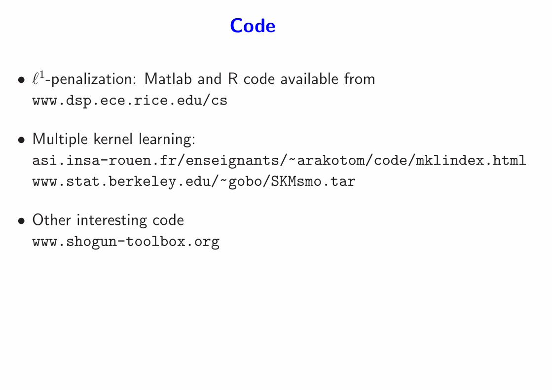
Code
• ℓ1-penalization: Matlab and R code available from
www.dsp.ece.rice.edu/cs
• Multiple kernel learning:
asi.insa-rouen.fr/enseignants/~arakotom/code/mklindex.html
www.stat.berkeley.edu/~gobo/SKMsmo.tar
• Other interesting code
www.shogun-toolbox.org