Learning to Trade

via Direct Reinforcement

by John Moody and Matthew Saffell

presented by Dustin Boswell

April 23, 2003

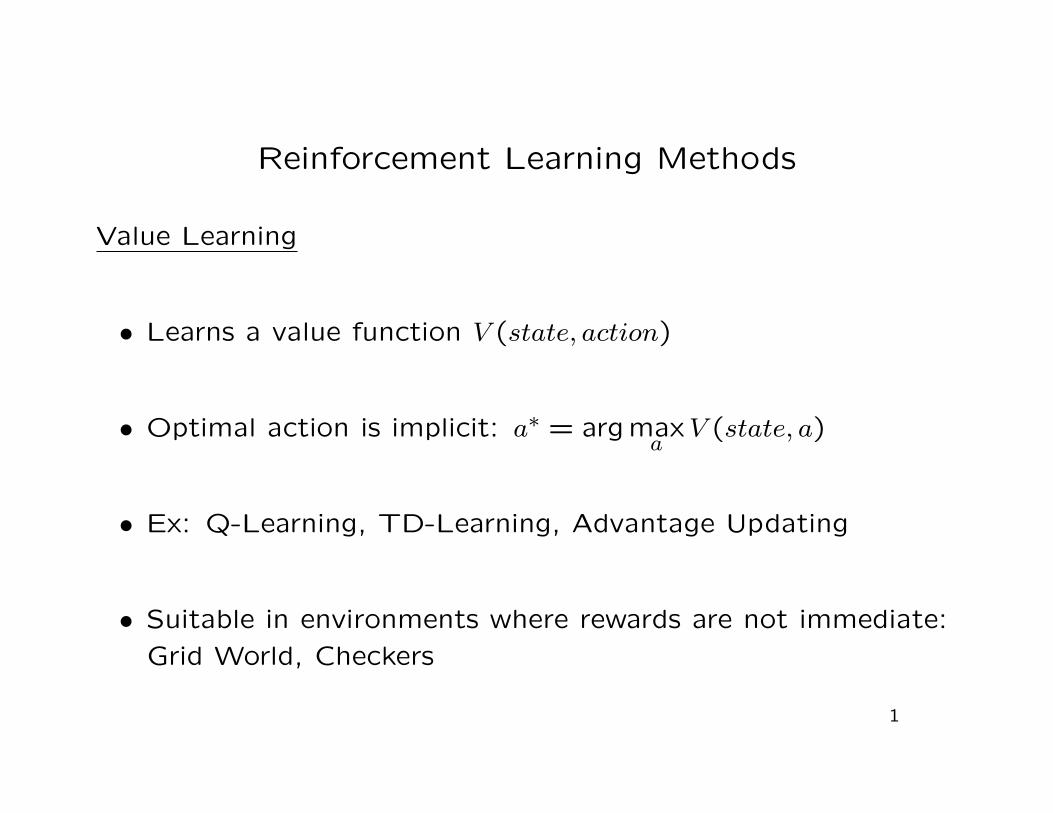
Reinforcement Learning Methods

Value Learning

• Learns a value function V (state, action)

• Optimal action is implicit: a∗ = argmaxa

V (state, a)

• Ex: Q-Learning, TD-Learning, Advantage Updating

• Suitable in environments where rewards are not immediate:

Grid World, Checkers

1

Reinforcement Learning Methods

Value Learning

• Learns

V (state, action)

• Optimal action is

implicit.

• Ex: Q-Learning

• Suitable for

delayed rewards

Direct Reinforcement Learning

• No value function

• Learns action policy directly

• Ex: Recurrent Reinforcement Learning

(RRL) given by Moody

• Suitable in environments where

rewards are immediate: Control

problems, stock markets

2

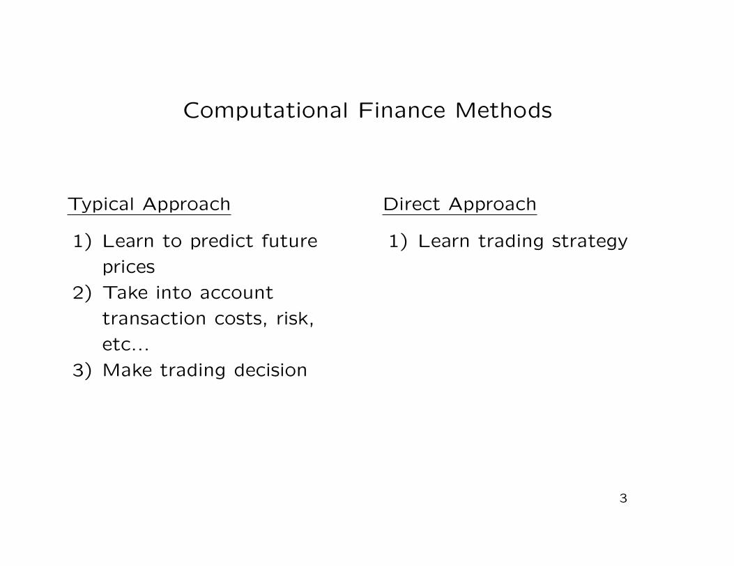
Computational Finance Methods

Typical Approach

1) Learn to predict future

prices

2) Take into account

transaction costs, risk,

etc...

3) Make trading decision

Direct Approach

1) Learn trading strategy

3

Notation

• Our agent trades fixed quantities of a security z.

• The price series is {z1, z2, . . . zt, . . . zT} and corresponding

price changes rt = zt − zt−1

• At each time step, our position is

Ft ∈ {long, neutral, short} = {+1,0,−1}

4

Notation (cont.)

• We wish to learn a trading strategy Ft = F (θt;Fi<t, It)

θ is the set of parameters we are learning

It = {zi≤t, etc...} is our Information at time t

• For example, a system with m + 1 “autoregressive inputs”:

Ft = sign(uFt−1 + v0rt + v1rt−1 + · · · vmrt−m + w)

θ = {u, vi, w}

• Whatever functional form used, F (θ) must be differentiable

(dF/dθ).

5

Profit & Wealth

• Daily Return: Rt = rt · Ft−1 − δ|Ft − Ft−1|δ is the transaction cost

• Total Profits: PT =∑T

t=1 Rt

i.e. no reinvesting

• Wealth: WT = W0 + PT

• Utility: UT = U(R1, . . . RT ;W0)

Ex: UT = WT measures profit without regard to risk

6

Measuring Utility: Sharpe Ratio

• Let UT be the Sharpe Ratio: ST = Average(Rt)StandardDeviation(Rt)

• To maximize UT , we will need an expression for dUT/dRt.

• But dST/dRt is hard to work with.

• Instead, Moody comes up with an approximation...

7

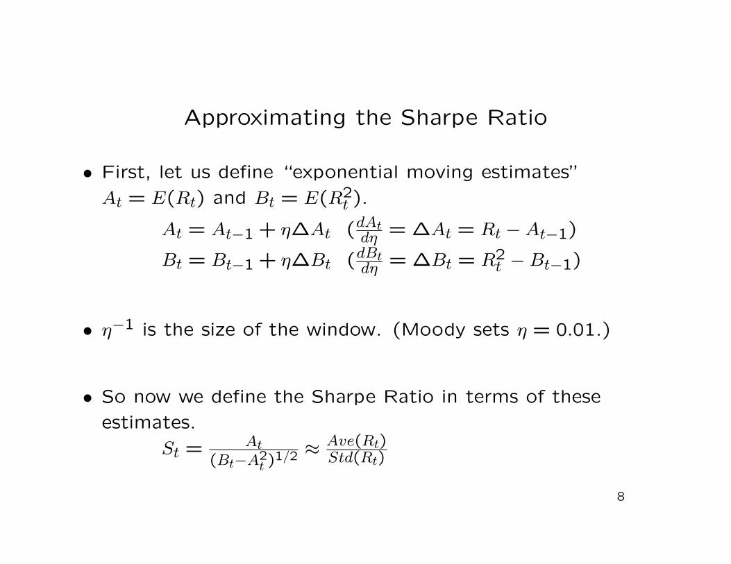
Approximating the Sharpe Ratio

• First, let us define “exponential moving estimates”

At = E(Rt) and Bt = E(R2t ).

At = At−1 + η∆At (dAtdη = ∆At = Rt − At−1)

Bt = Bt−1 + η∆Bt (dBtdη = ∆Bt = R2

t − Bt−1)

• η−1 is the size of the window. (Moody sets η = 0.01.)

• So now we define the Sharpe Ratio in terms of these

estimates.

St = At

(Bt−A2t )

1/2 ≈Ave(Rt)Std(Rt)

8

Approximating the Sharpe Ratio (cont.)

• Now Taylor expand St about η ( not obvious why, but it

helps the algebra ).

St ≈ St−1 + ηdStdη |η=0 + O(η2)

• Ignore O(η2). Notice only the center term depends on Rt.

This lets us say dStdRt

≈ ddRt

ηDt

Dt ≡ dStdη = d

dηAt

(Bt−A2t )

1/2

Dt ≡Bt−1∆At−1

2At−1∆Bt

(Bt−1−A2t−1)

3/2

9

Measuring Utility: Sharpe Ratio (cont.)

• Finally, we arrive atdDtdRt

=Bt−1−At−1Rt

(Bt−1−A2t−1)

3/2

• Hence we’ve gotten our expression :dUtdRt

= dStdRt

≈ ηdDtdRt

• Notice the largest improvement to Ut is when

R∗t = Bt−1/At−1

• So the Sharpe Ratio penalizes gains larger than R∗t !

10

Measuring Utility: Sterling Ratio

• SterlingT = Average Yearly ReturnMaximum Draw Down

• MDD = maxi<j(zi − zj)

where j − i ≤ 1 year

• Useful for mutual fund managers wanting to minimize

displeased customers

• Unfortunately, difficult to deal with analytically

11

Measuring Utility: Double Deviation Ratio

• DDRT = Average(Rt)DDT

• DDT =(1T

∑Tt=1 min{Rt,0}2

)1/2

• DDR rewards large average positive returns,

penalizes “risky” (large negative) returns

12

Learning Parameters through Gradient Ascent

• Given Ft(θ) we want to adjust θ to maximize UT :

dUT (θ)dθ =

T∑t=1

dUTdRt

{dRtdFt

dFtdθ + dRt

dFt−1

dFt−1dθ

}∆θ = ρdUT (θ)

dθ ( ρ is the learning rate )

• dUTdRt

: we saw this from before

• dRtdFt

: easy to determine

• dFtdθ : dFt

dθ = ∂Ft∂θ + ∂Ft

∂Ft−1

dFt−1dθ recursively . . .

13

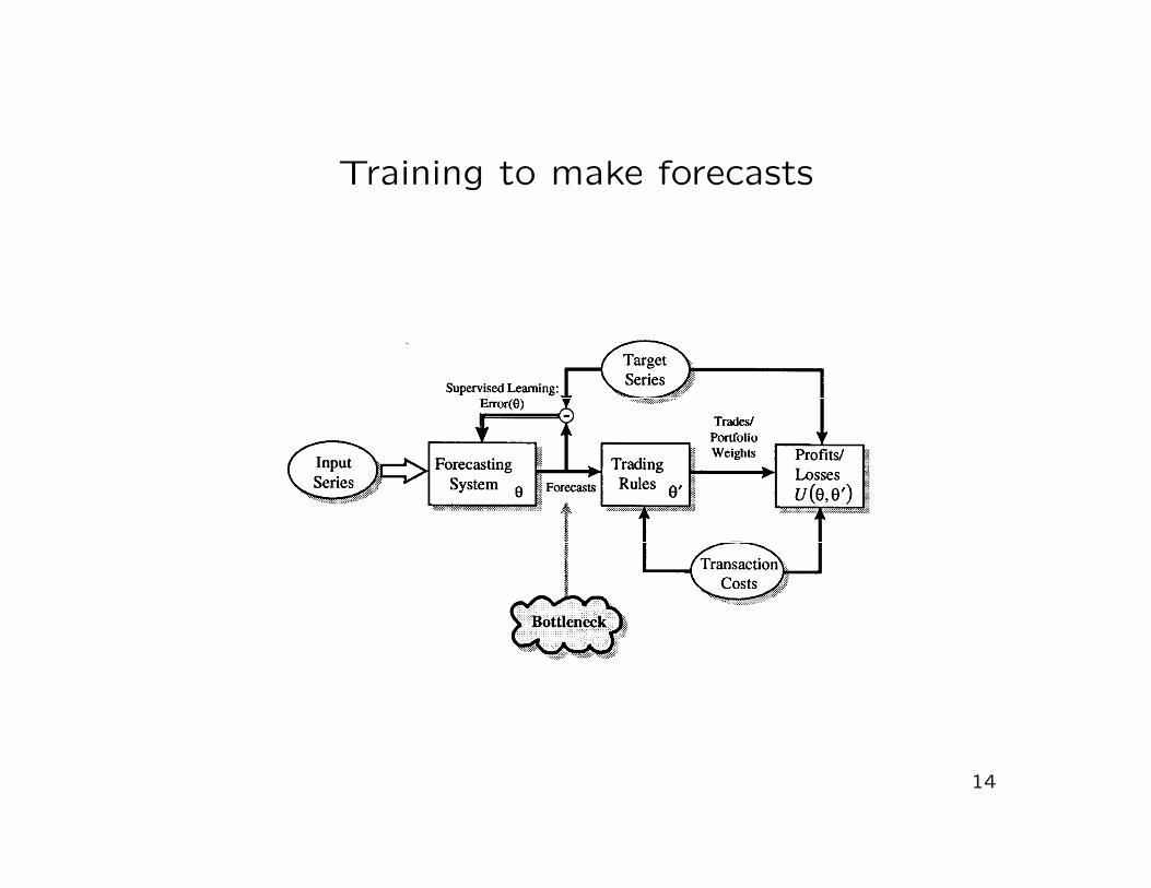
Training to make forecasts

14

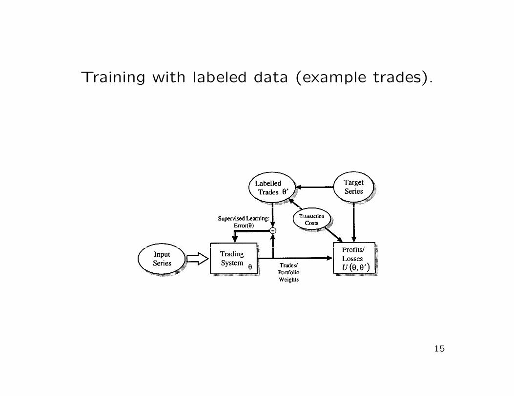
Training with labeled data (example trades).

15

RRL “Direct Reinforcement” Approach

16

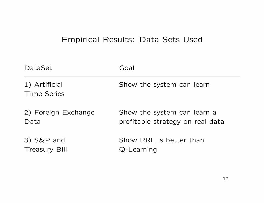
Empirical Results: Data Sets Used

DataSet Goal

1) Artificial Show the system can learn

Time Series

2) Foreign Exchange Show the system can learn a

Data profitable strategy on real data

3) S&P and Show RRL is better than

Treasury Bill Q-Learning

17

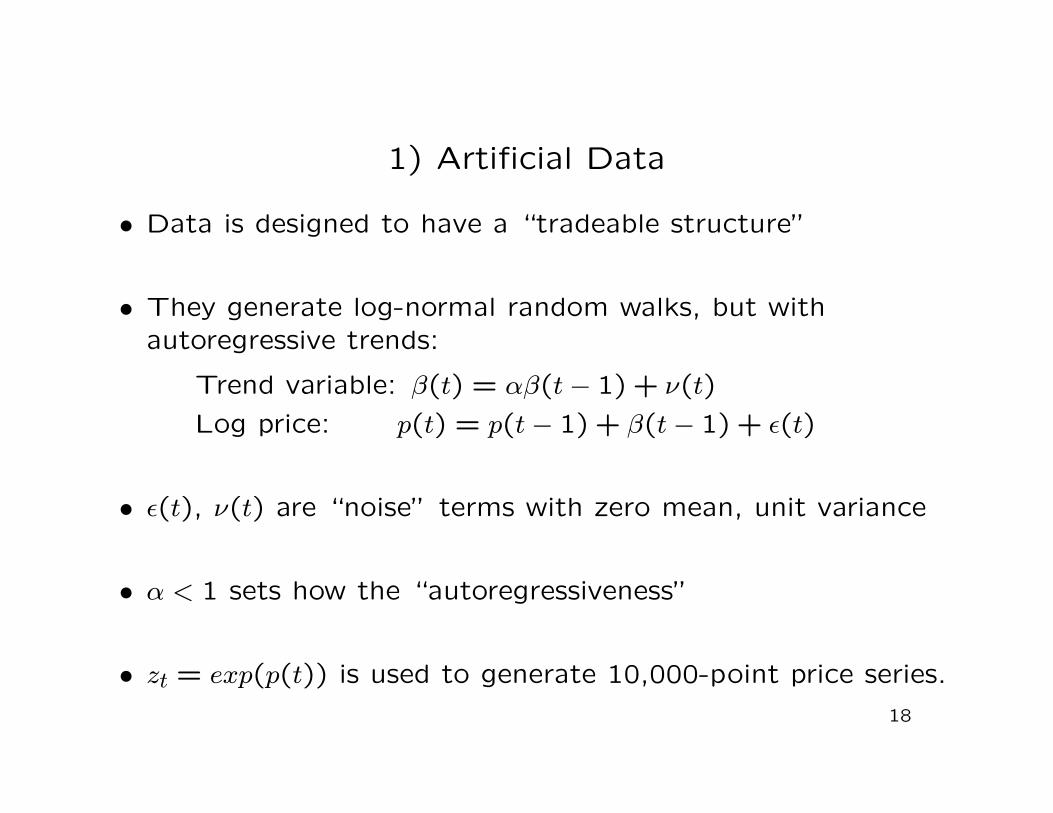
1) Artificial Data

• Data is designed to have a “tradeable structure”

• They generate log-normal random walks, but withautoregressive trends:

Trend variable: β(t) = αβ(t− 1) + ν(t)

Log price: p(t) = p(t− 1) + β(t− 1) + ε(t)

• ε(t), ν(t) are “noise” terms with zero mean, unit variance

• α < 1 sets how the “autoregressiveness”

• zt = exp(p(t)) is used to generate 10,000-point price series.

18

1) Artificial Data - System Details

• The trading function has autoregressive inputs (matches

the data):

Ft = sign(uFt−1 + v0rt + v1rt−1 + · · · v7rt−7 + w)

• Transaction cost: δ = 0.5%

• Learns to maximize the Differential Sharpe Ratio

19

Artificial Prices, and Results

20

Histograms of Artificial Data and Results

21

Artificial Data (continued)

• How do transaction costs affect trading performance?

• Repeat the previous experiments 100 times...

try δ = 0.2%,0.5%,1.0%

• Hypothesis: lower costs should allow:

- more trading

- more profits

- better Sharpe Ratio

22

Boxplots of how transaction costs

affect profits

23

Boxplots of how transaction costs

affect trading frequency

24

Boxplots of how transaction costs

affect Sharpe Ratio

25

2) Foreign Exchange Data

• US Dollar vs. British Pound

• 8 months of data (half-hour quotes) during 1996

• Same autoregressive inputs as Artificial Data experiment?(the paper was unclear)

• The system is trained to maximize theDownside Deviation Ratio.

• Transaction cost is the bid-ask spread(which has a typical average but is not fixed).

26

Foreign Exchange Prices, and Results

27

Foreign Exchange Result Summary

• 15% annualized return, Sharpe Ratio of 2.3

• (S&P index gets roughly 15% return, Sharpe < 1)

• Trading frequency: trades are made roughly once every 5

hours

• It’s difficult to say how well this would have done in real

world environment (since you can’t simulate all market

frictions).

28

3) US Stock Market Data: Q-Trader against

RRL-Trader

• S&P vs. Treasury Bill

• 25 years of data: 1970-1994

• System is trained on previous 20 years (sliding window)

• The Information It also includes macroeconomic data

• Also implement Q-Learning (actually, a variant calledAdvantage Updating) to compare.

29

Q-Trader vs. RRL-Trader Results

30

Q-Trader vs. RRL-Trader Results (continued)

31

Conclusions

• Moody makes the case that RRL is better than Q-Learning

for trading since it is a simpler approach.

(Simpler is better - a recurring theme in this class.)

• I’m not sure I agree personally with some of his methods.

• Moody has set up an interesting method for learning

directly, but hasn’t addressed the problem of choosing a

good trading model.

32