Learning to Speed Up Search

Bart Selman and Wei Wei

Introduction

In this talk, we’ll survey some promising recent developments in using learning methods to speed up search

General methodology: (1) Use machine learning techniques to uncover hidden structure of the search space. (2) Use this information to speed up search.

General ObservationsApproaches fall into two classes:A) Work in the machine learning community. We

will discuss three examples. Promising, but in general not compared to best other solution methods.

B) Approaches coming out of search / SAT community. Powerful but do not explicitly use state-of-the-art learning methods.

We will compare and contrast A & B.

Work From the Machine Learning Community

Three examples

Learn good starting states for local search.

STAGE --- Boyan & Moore 1998

Learn structure of search space directly.

MIMIC --- Bonet et al. 1996

Learn new objective function that is easier for local search.

Zhang & Dietterich 1995.

I) STAGE algorithmBoyan and Moore 1998

Idea: more features of the current state may help local search

Task: to incorporate these features into improved evaluation functions, and help guide search

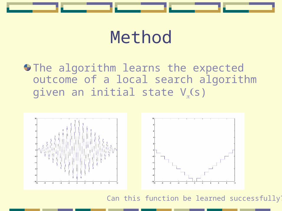
Method

The algorithm learns the expected outcome of a local search algorithm given an initial state Vs)

Can this function be learned successfully?

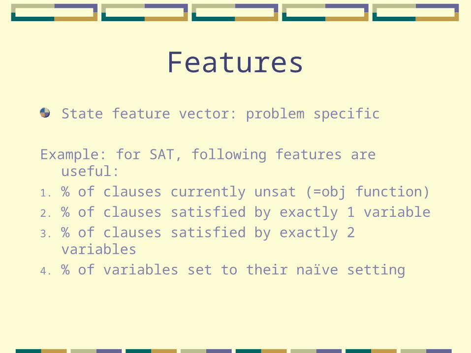
Features

State feature vector: problem specific

Example: for SAT, following features are useful:

1. % of clauses currently unsat (=obj function)

2. % of clauses satisfied by exactly 1 variable

3. % of clauses satisfied by exactly 2 variables

4. % of variables set to their naïve setting

Learner

Fitter: can be any function approximator; polynomial regression is used in practice.

Training data: generated on the fly; every LS trajectory produces a series of new training data.

Restrictions on : it must terminate; it must be Markovian.

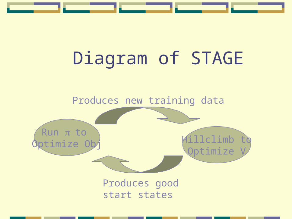
Diagram of STAGE

Run to Optimize Obj Hillclimb to

Optimize V

Produces new training data

Produces good start states

Results

Works on many domain, such as bin-packing, channel routing, SAT

On SAT, reduces the number of unsat clauses on par32 benchmarks (from 9 to 1) when STAGE learner is introduced to WalkSAT

Discussion

Is the learned function a good approximation to V(s)? – Somewhat unclear.

(“worrisome”: linear regression performs better than quadratic regression, which should give a better approximation. Learning does help however.)

Why not learn a better objective function and search on that function directly (clause weighing)?

(Zhang and Dietterich, 3rd example.)

II) MIMIC De Bonet et al, 1997

MIMIC learns a probability density distribution over the search space by repeated and “clever” sampling.

The purpose of retaining this density distribution is to communicate information about the search space from one iteration of the search to the next.

The idea in more detail

If we know nothing about a search space, we look for its minimum by generating points from a uniform distribution over all inputs

Less work is necessary if we know the distribution pθ(x), which is uniformly distributed over those inputs with objective O(x) θ, and has a probability of 0 elsewhere

In particular, the task is trivial when we when the distribution pθ’(x), in which θ’= minx O(x)

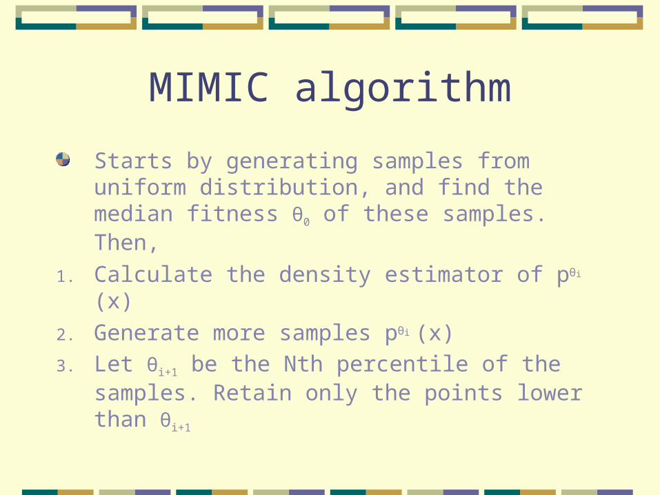
MIMIC algorithm

Starts by generating samples from uniform distribution, and find the median fitness θ0 of these samples. Then,

1. Calculate the density estimator of pθi (x)

2. Generate more samples pθi (x)

3. Let θi+1 be the Nth percentile of the samples. Retain only the points lower than θi+1

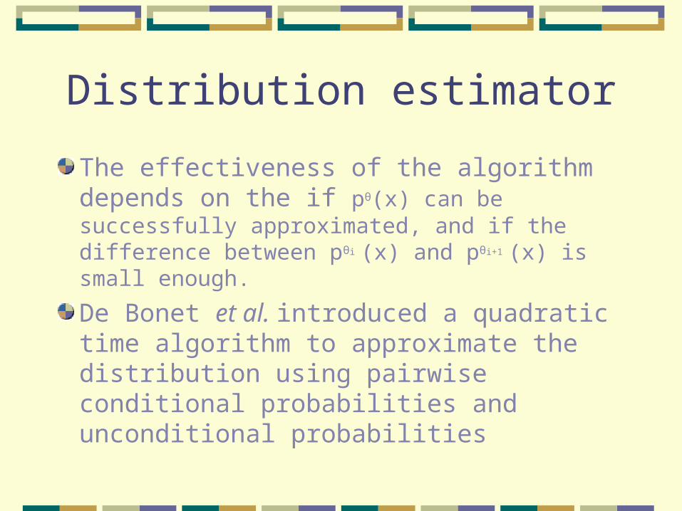
Distribution estimator

The effectiveness of the algorithm depends on the if pθ(x) can be successfully approximated, and if the difference between pθi (x) and pθi+1 (x) is small enough.

De Bonet et al. introduced a quadratic time algorithm to approximate the distribution using pairwise conditional probabilities and unconditional probabilities

Approximation

The true joint probability distribution is p(X) = p(X1|X2…Xn)p(X2|X3…Xn)…p(Xn-1|Xn)p(Xn)

Given a permutation of 1…n, =i1i2…in,

Letp’(X) = p(Xi1|Xi2)p(Xi2|Xi3)…p(Xin-1|Xin)p(Xin)

Ideally, we want to search over all ’s to find the closest one to the true distribution, but there are too many of them

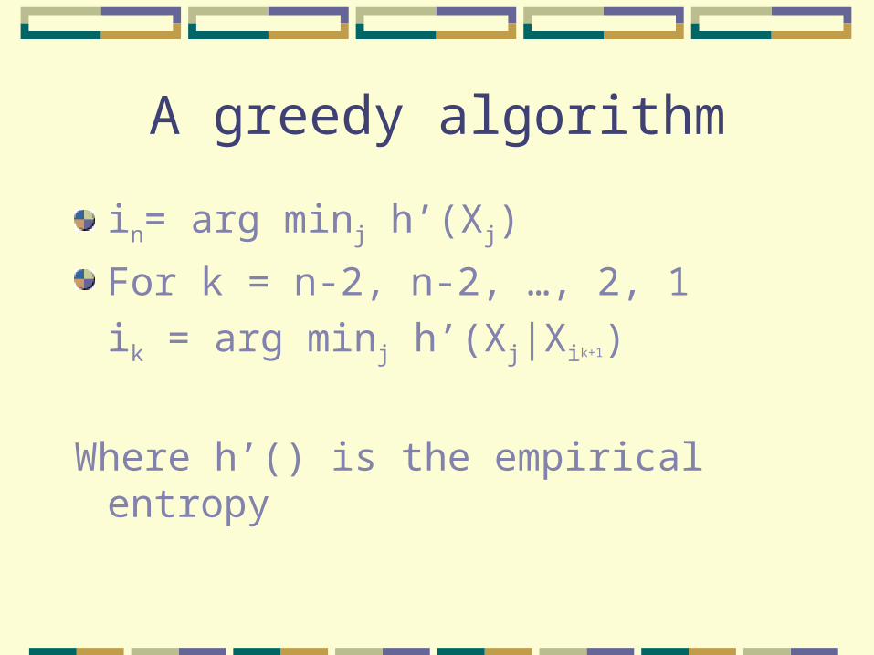
A greedy algorithm

in= arg minj h’(Xj)

For k = n-2, n-2, …, 2, 1

ik = arg minj h’(Xj|Xik+1)

Where h’() is the empirical entropy

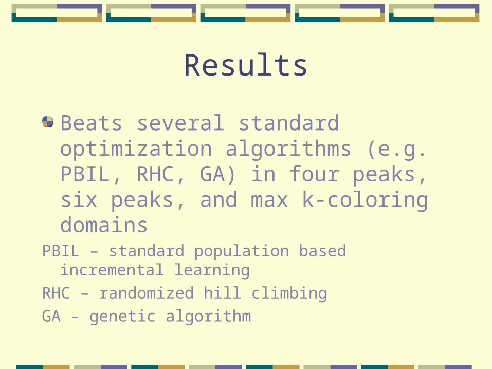
Results

Beats several standard optimization algorithms (e.g. PBIL, RHC, GA) in four peaks, six peaks, and max k-coloring domains

PBIL – standard population based incremental learning

RHC – randomized hill climbing

GA – genetic algorithm

III) Reinforcement learning for scheduling Zhang and Dietterich, 1995

Domain: space shuttle payload processing of NASA

To schedule several jobs; each job has a set of partially-ordered tasks; each task has a duration and a list of resource requirements

35 different resources, each of which has many units available. However, the units are divided into pools, and a task has to draw its need of a resource from a single pool

NASA domain continued

Each job has a fixed launch date, but no starting and ending dates. Most of its tasks are to be performed before the launch date Others take place after the launch dateGoal: find a feasible schedule of the jobs with minimum durationThe algorithm must be able to repair a schedule in case unforeseen event happens

Approach

Critical path: the tightest schedule without considering the resource constraints. (the only consideration is the partial ordering of the tasks.)Resource dilation factor (RDF): can be regarded as a scale-independent measure of the length of the scheduleActions: Reassign-Pool and Move

Approach, continued

Start from the critical path

Reinforce function R(s, a, s’) is equal to –0.001 if s’ is not a feasible state. R(s, a, s’) = -RDF(s’, s0) otherwise.

Reinforcement Learning

We learn a policy , which tells us what action (“local search move”) to take in every state

We can define a value function f, and f(s) is the cumulative reward we can get from s on if we follow We hope to learn the optimal policy *, but we can learn f (denoted as f*) instead, because we can look one step ahead

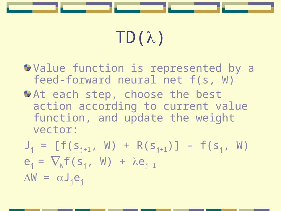
TD()

Value function is represented by a feed-forward neural net f(s, W)At each step, choose the best action according to current value function, and update the weight vector:

Jj = [f(sj+1, W) + R(sj+1)] – f(sj, W)

ej = Wf(sj, W) + ej-1

W = Jjej

Results

Compared with iterative repair (IR) method previously used in the domain, temporal difference (TD) scheduling finds a schedule 3.9% shorter, which translates to 14 days if the schedule lasts 1 year

Approaches from the Search/SATCommunity

Two Strategies

Clause learning. Both for backtrack search and for local search.

Clause weighing. For local search.

Both strategies can be viewed as “changing the objective function” (while maintaining global optima).

Clause learning

DPLL – branch and backtracking

Learning as a pruning method. Generate implied clauses during search, and add them to the clauses database

Clauses are generated by conflict analysis

The technique is employed by state-of-the-art SAT solvers, e.g. Chaff, rel-sat, GRASP

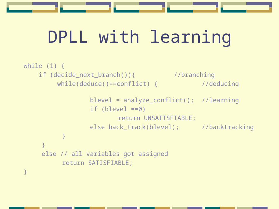
DPLL with learning

while (1) { if (decide_next_branch()){ //branching while(deduce()==conflict) { //deducing

blevel = analyze_conflict(); //learningif (blevel ==0)

return UNSATISFIABLE;else back_track(blevel); //backtracking

} } else // all variables got assigned

return SATISFIABLE;}

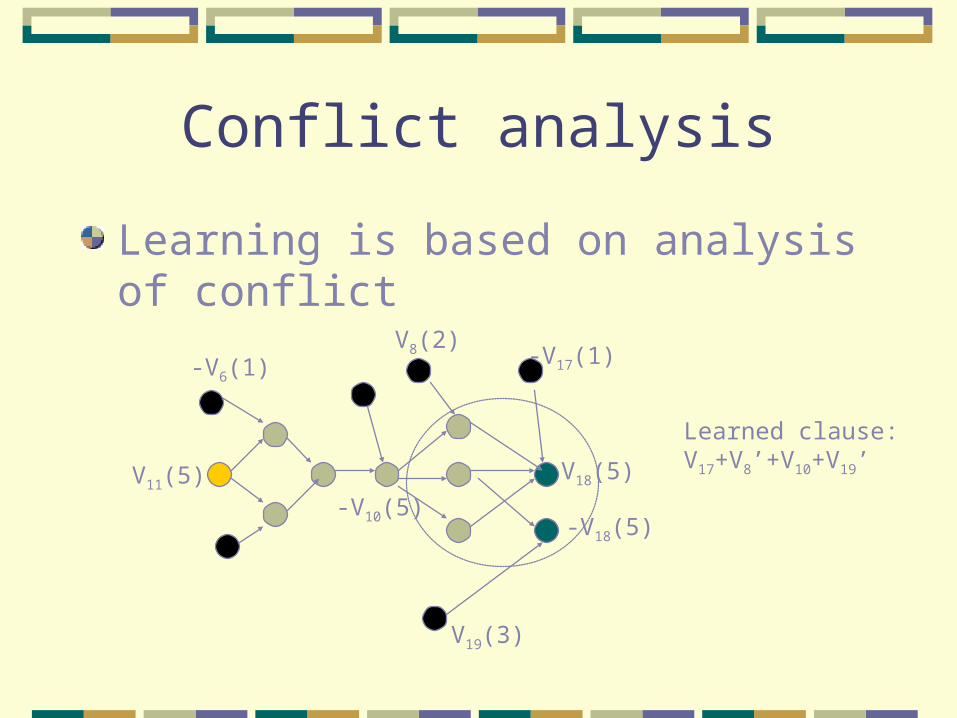
Conflict analysis

Learning is based on analysis of conflict

-V6(1)

V11(5) V18(5)

-V18(5)

-V17(1)V8(2)

-V10(5)

V19(3)

Learned clause:V17+V8’+V10+V19’

Clause learning

Many schemes available for generating clauses

Restarting is helpful in DPLL solvers (Gomes et al, 1995). When restarted, all learned clauses from previous runs are kept

Clause Learning --- Local Search

Similar to clause learning in DPLL solvers, adding new clauses during local search.

(Cha and Iwama, 1996)Clauses added are one-step resolvents that are unsat at the local minimaIt has similar effects as increasing weights of unsat clauses.New approach: add clauses to capture long range structure to speed up local search.

(Wei Wei and Selman, CP 2002)

Clause weighing

Used by local search solvers as a way to “memorize” traps it has encountered.

(Morris 1993; Kautz & Selman 1993)

When search gets stuck, update the weight of each clauseEffectively change the landscape of search space during search (learn a better objective function)Used by a range of efficient stochastic LS algorithms, e.g. DLM (Wu and Wah, 2000), ESG (Schuurmans et al, 2001)

Summary

Recent developments in Machine Learning Community for using learning to speed up search are encouraging.

However, so far, comparisons have been done only against relatively naïve search methods.

Little (or no) follow-up in search/SAT community.

Success of relatively ad-hoc strategies such as clause learning and weighing suggests that more advanced machine learning ideas may have a significant pay-off.

Key idea: Discover (“learn”) hidden structure in underlying search space.

It appears time to re-evaluate the machine learning approaches by incorporating the

ideas in state-of-the-art solvers.