Learning to Search

Henry Kautz

University of Washingtonjoint work with

Dimitri Achlioptas, Carla Gomes, Eric Horvitz, Don Patterson, Yongshao Ruan, Bart Selman

CORE – MSR, Cornell, UW

Speedup Learning

Machine learning historically considered Learning to classify objects Learning to search or reason more efficiently

Speedup Learning Speedup learning disappeared in mid-90’s

Last workshop in 1993 Last thesis 1998

What happened? It failed. It succeeded. Everyone got busy doing something else.

It failed.

Explanation based learning Examine structure of proof trees Explain why choices were good or bad (wasteful) Generalize to create new control rules

At best, mild speedup (50%) Could even degrade performance

Underlying search engines very weak Etzioni (1993) – simple static analysis of next-state

operators yielded as good performance as EBL

It succeeded.

EBL without generalization Memoization No-good learning SAT: clause learning

Integrates clausal resolution with DPLL Huge win in practice!

Clause-learning proofs can be exponentially smaller than best DPLL (tree shaped) proof

Chaff (Malik et al 2001) 1,000,000 variable VLSI verification problems

Everyone got busy.

The something else: reinforcement learning. Learn about the world while acting in the world Don’t reason or classify, just make decisions What isn’t RL?

Another path

Predictive control of search Learn statistical model of behavior of a problem solver

on a problem distribution Use the model as part of a control strategy to improve

the future performance of the solver Synthesis of ideas from

Phase transition phenomena in problem distributions Decision-theoretic control of reasoning Bayesian modeling

Big Picture

ProblemInstances

Solver

static features

runtime

Learning /Analysis

PredictiveModel

dynamic features

resource allocation / reformulation

control / policy

Case Study 1: Beyond 4.25

ProblemInstances

Solver

static features

runtime

Learning /Analysis

PredictiveModel

Phase transitions & problem hardness

Large and growing literature on random problem distributions

Peak in problem hardness associated with critical value of some underlying parameter

3-SAT: clause/variable ratio = 4.25 Using measured parameter to predict hardness of

a particular instance problematic! Random distribution must be a good model of actual

domain of concern Recent progress on more realistic random

distributions...

Quasigroup Completion Problem (QCP)

NP-Complete Has structure is similar to that of real-world problems -

tournament scheduling, classroom assignment, fiber optic routing, experiment design, ...

Can generate hard guaranteed SAT instances (2000)

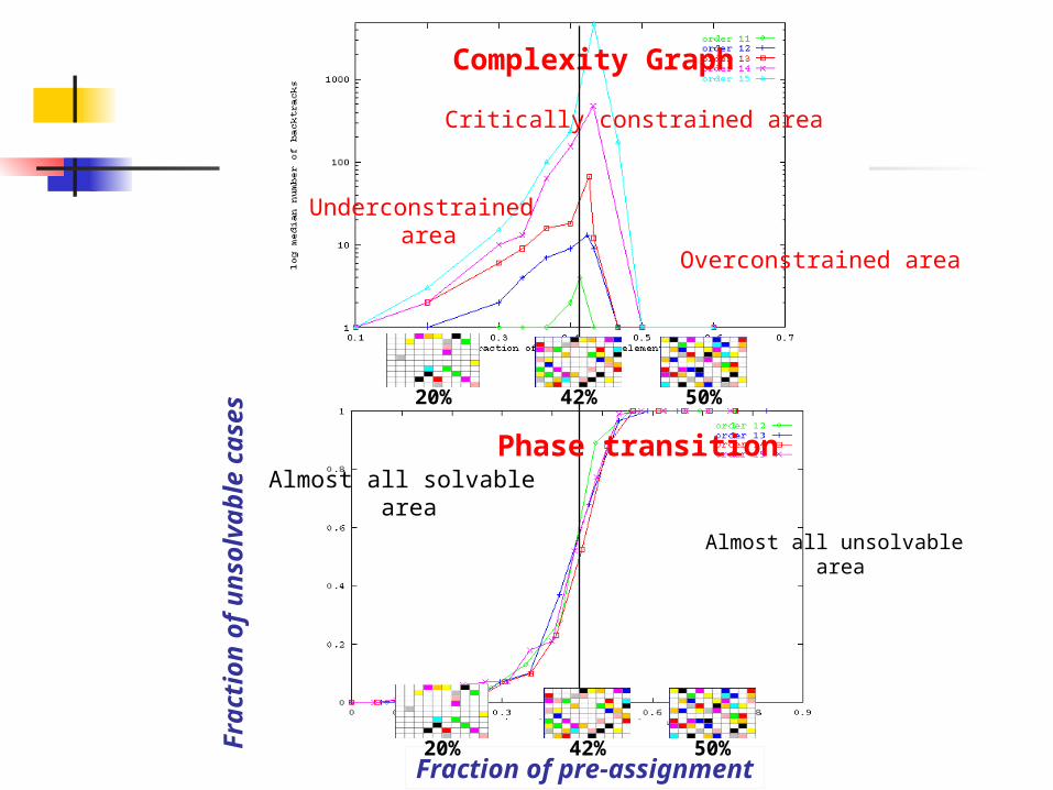
Phase Transition

Almost all unsolvable area

Fraction of pre-assignment

Fra

ctio

n o

f u

nso

lvab

le c

ases

Almost all solvable area

Complexity Graph

Phase transition

42% 50%20%

42% 50%20%

Underconstrained area

Critically constrained area

Overconstrained area

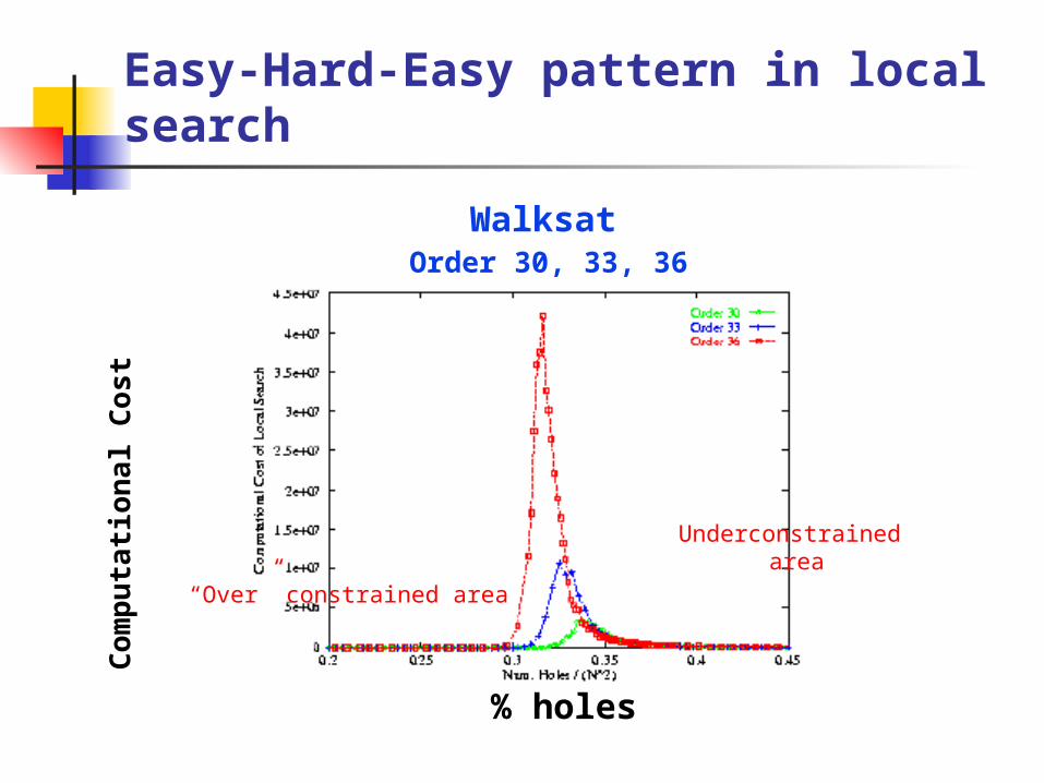
Easy-Hard-Easy pattern in local search

% holes

Co

mp

uta

tio

na

l Co

st

WalksatOrder 30, 33, 36

“Over” constrained area

Underconstrained area

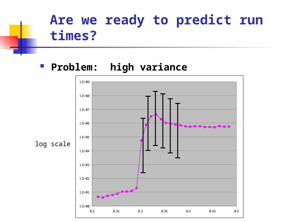
Are we ready to predict run times?

Problem: high variance

1.E+00

1.E+01

1.E+02

1.E+03

1.E+04

1.E+05

1.E+06

1.E+07

1.E+08

1.E+09

0.2 0.25 0.3 0.35 0.4 0.45 0.5

log scale

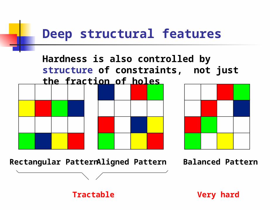
Deep structural features

Rectangular Pattern Aligned Pattern Balanced Pattern

Tractable Very hard

Hardness is also controlled by structure of constraints, not just the fraction of holes

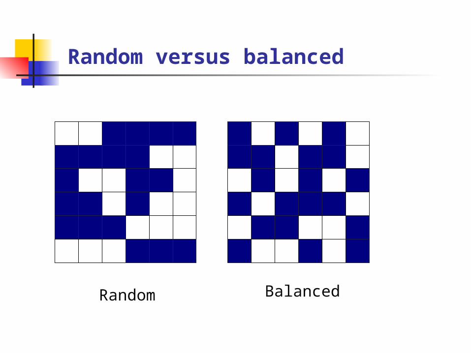
Random versus balanced

BalancedRandom

Random versus balanced

0.E+00

1.E+07

2.E+07

3.E+07

4.E+07

5.E+07

6.E+07

7.E+07

0.2 0.25 0.3 0.35 0.4 0.45 0.5

Balanced

Random

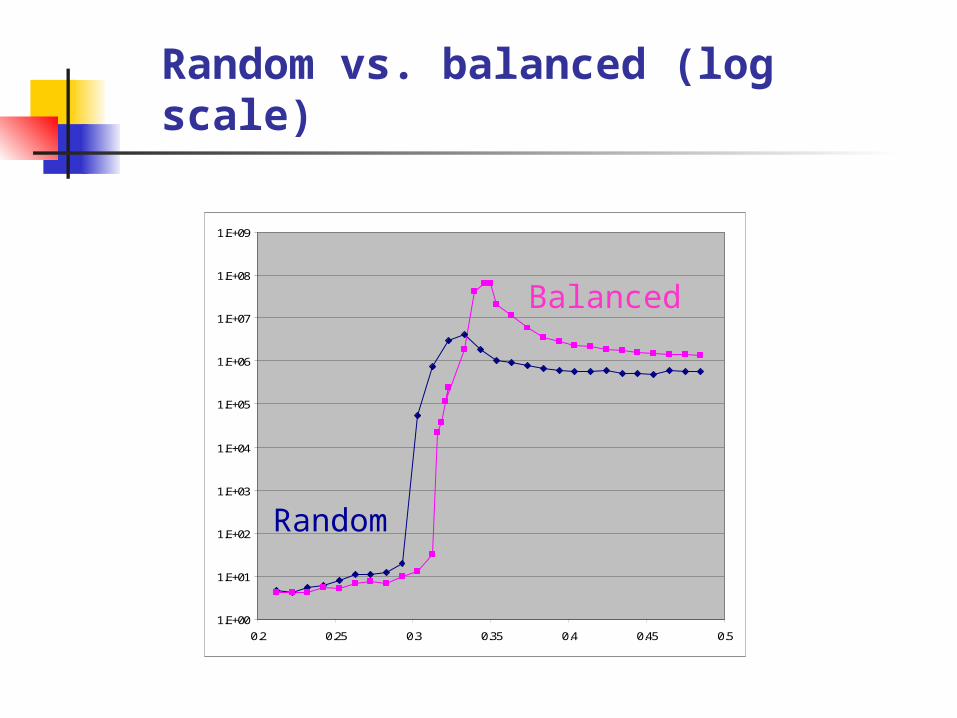
Random vs. balanced (log scale)

1.E+00

1.E+01

1.E+02

1.E+03

1.E+04

1.E+05

1.E+06

1.E+07

1.E+08

1.E+09

0.2 0.25 0.3 0.35 0.4 0.45 0.5

Balanced

Random

Morphing balanced and random

Mixed Model - Walksat

0

10

20

30

40

50

60

70

80

90

100

0.00% 20.00% 40.00% 60.00% 80.00% 100.00%

Percent random holes

Tim

e (s

econds)

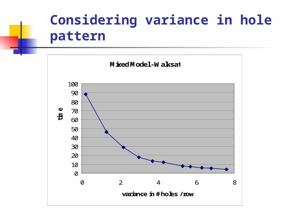
Considering variance in hole pattern

Mixed Model - Walksat

0

10

20

30

40

50

60

70

80

90

100

0 2 4 6 8

variance in # holes / row

tim

e

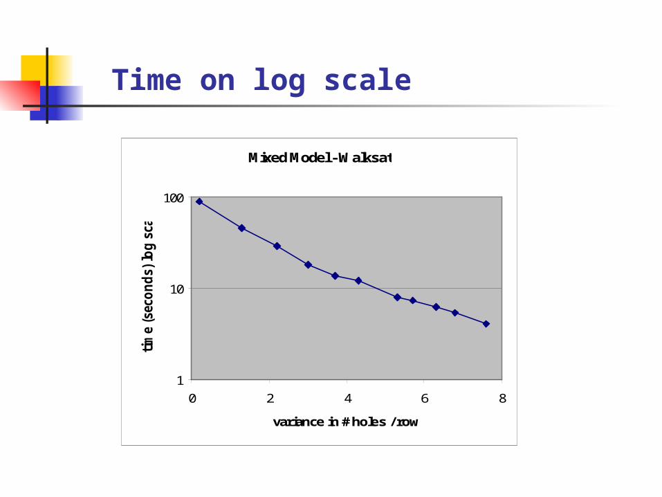
Time on log scale

Mixed Model - Walksat

1

10

100

0 2 4 6 8

variance in # holes / row

tim

e (s

econds)

log s

cale

Effect of balance on hardness

Balanced patterns yield (on average) problems that are 2 orders of magnitude harder than random patterns

Expected run time decreases exponentially with variance in # holes per row or column

E(T) = C-k

Same pattern (differ constants) for DPPL! At extreme of high variance (aligned model) can

prove no hard problems exist

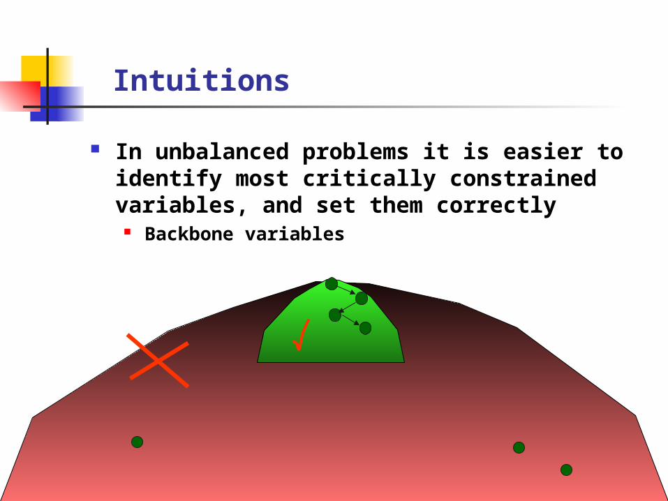
Intuitions

In unbalanced problems it is easier to identify most critically constrained variables, and set them correctly

Backbone variables

Are we done?

Unfortunately, not quite. While few unbalanced problems are hard, “easy”

balanced problems are not uncommon To do: find additional structural features that

signify hardness Introspection Machine learning (later this talk) Ultimate goal: accurate, inexpensive prediction of

hardness of real-world problems

Case study 2: AutoWalksat

ProblemInstances

Solver

runtime

Learning /Analysis

PredictiveModel

dynamic features

control / policy

Walksat

Choose a truth assignment randomlyWhile the assignment evaluates to false

Choose an unsatisfied clause at randomIf possible, flip an unconstrained variable in that clauseElse with probability P (noise)

Flip a variable in the clause randomlyElse flip the variable in the clause which causes the

smallest number of satisfied clauses to become unsatisfied.

Performance of Walksat is highly sensitive to the setting of P

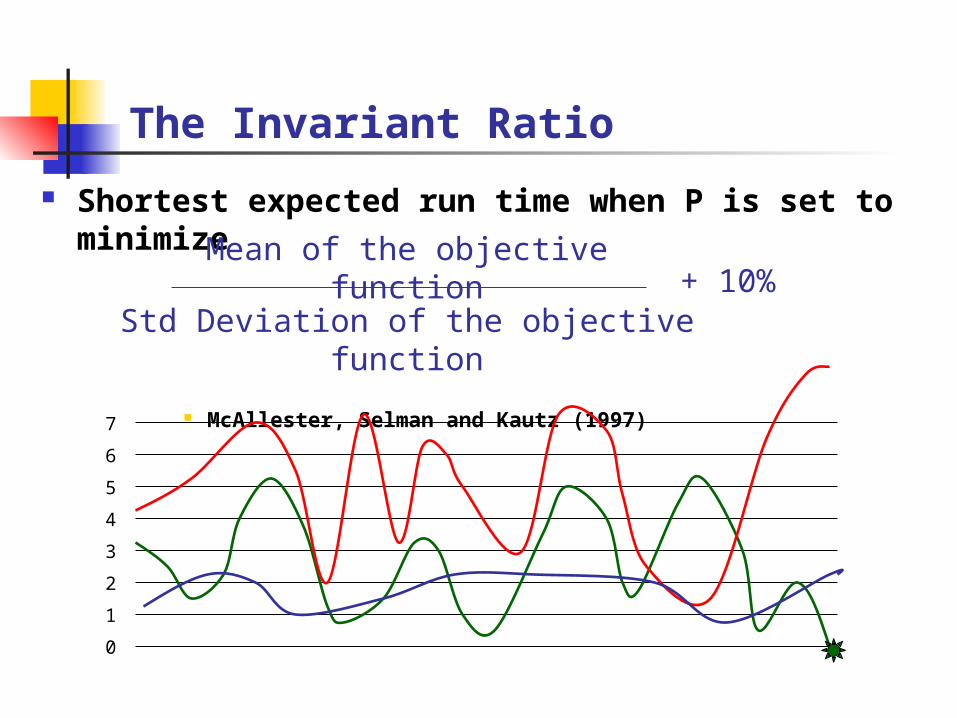
Shortest expected run time when P is set to minimize

McAllester, Selman and Kautz (1997)

The Invariant Ratio

Mean of the objective function

Std Deviation of the objective function

0

1

2

3

4

5

6

7

+ 10%

Automatic Noise Setting

Probe for the optimal noise level

Bracketed Search with Parabolic Interpolation No derivatives required Robust to stochastic variations Efficient

Hard random 3-SAT

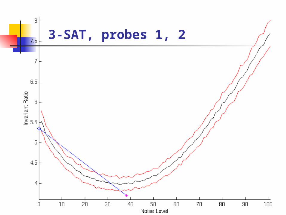
3-SAT, probes 1, 2

3-SAT, probe 3

3-SAT, probe 4

3-SAT, probe 5

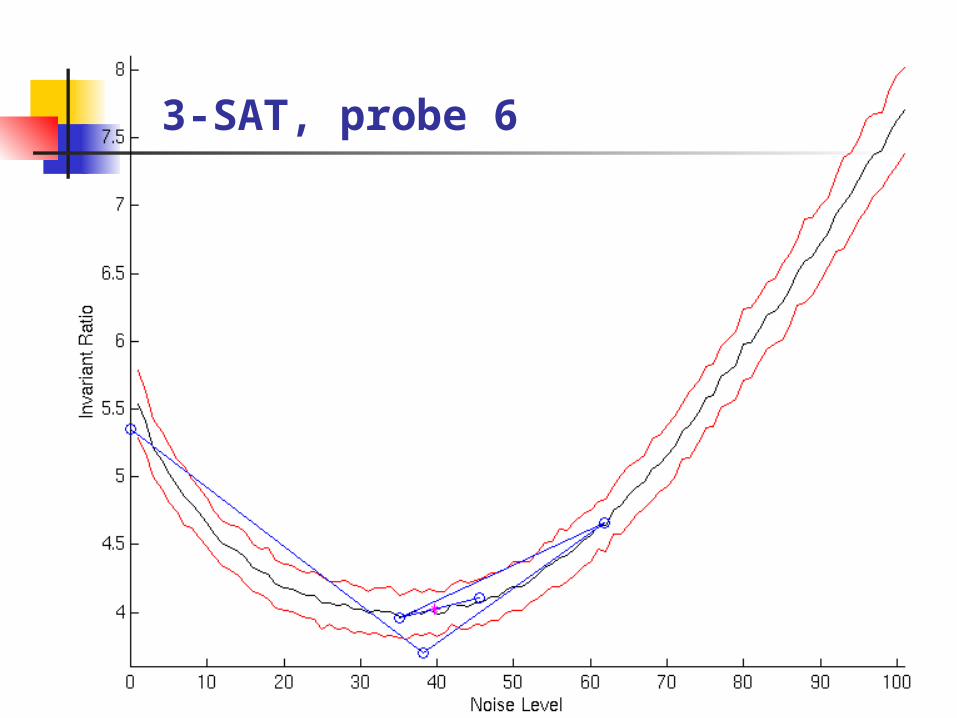
3-SAT, probe 6

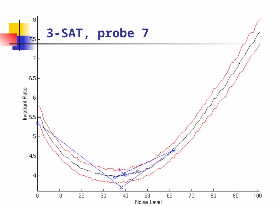
3-SAT, probe 7

3-SAT, probe 8

3-SAT, probe 9

3-SAT, probe 10

Summary: random, circuit test, graph coloring, planning

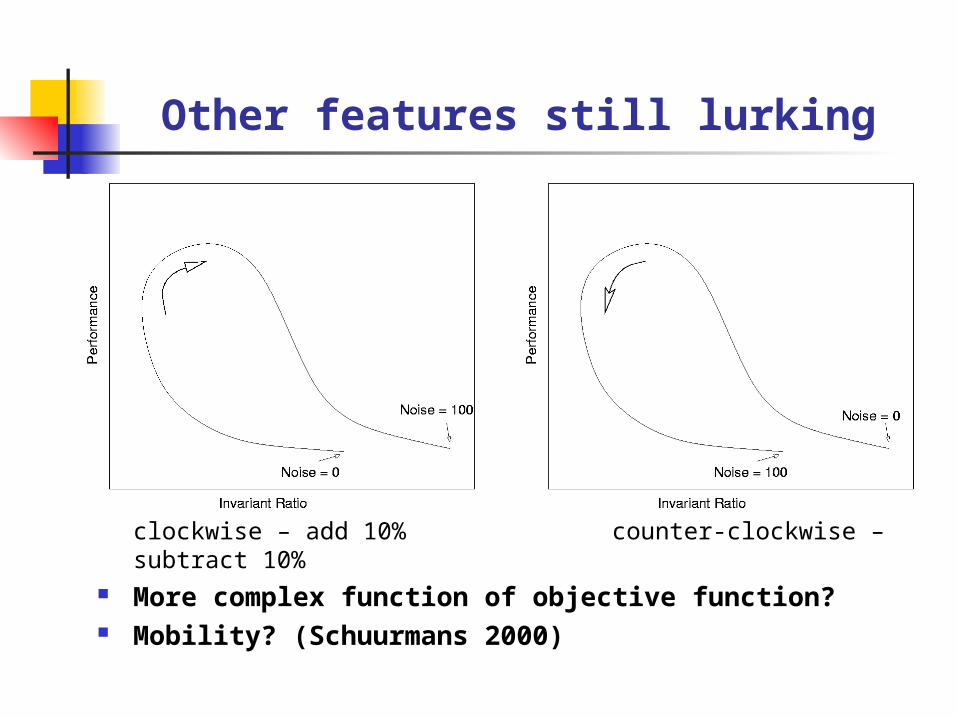
Other features still lurking

clockwise – add 10% counter-clockwise – subtract 10%

More complex function of objective function? Mobility? (Schuurmans 2000)

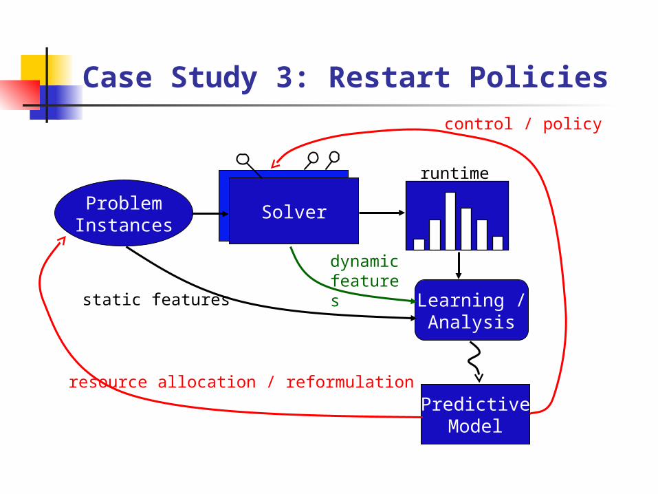
Case Study 3: Restart Policies

ProblemInstances

Solver

static features

runtime

Learning /Analysis

PredictiveModel

dynamic features

resource allocation / reformulation

control / policy

BackgroundBackground

Backtracking search methods often exhibit a remarkable variability in performance between: different heuristics same heuristic on different instances different runs of randomized heuristics

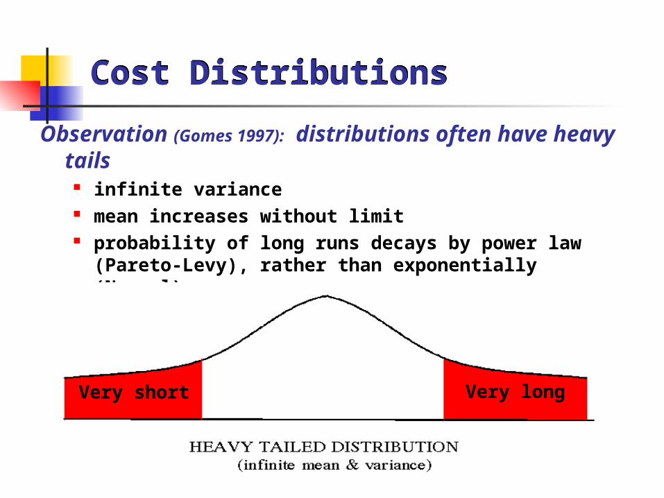
Cost DistributionsCost Distributions

Observation (Gomes 1997): distributions often have heavy tails

infinite variance mean increases without limit probability of long runs decays by power law (Pareto-Levy),

rather than exponentially (Normal)

Very short Very long

Randomized Restarts

Solution: randomize the systematic solver Add noise to the heuristic branching (variable

choice) function Cutoff and restart search after a some number of

steps Provably eliminates heavy tails Very useful in practice

Adopted by state-of-the art search engines for SAT, verification, scheduling, …

Effect of restarts on expected solution time (log scale)

1000

10000

100000

1000000

1 10 100 1000 10000 100000 1000000

log( cutoff )

log

( b

ackt

rack

s )

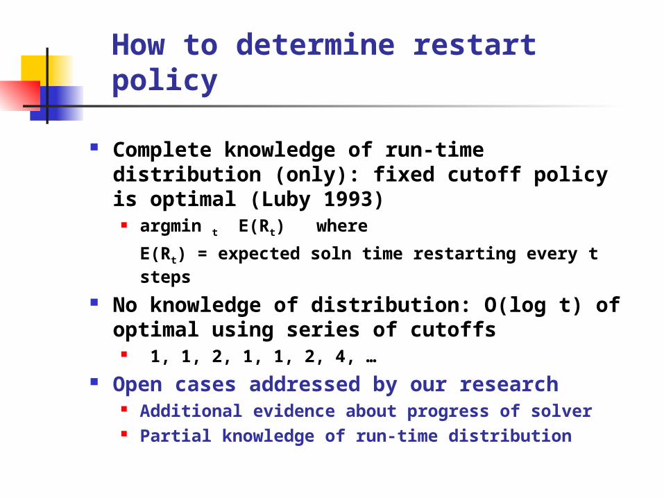
How to determine restart policy

Complete knowledge of run-time distribution (only): fixed cutoff policy is optimal (Luby 1993)

argmin t E(Rt) where

E(Rt) = expected soln time restarting every t steps

No knowledge of distribution: O(log t) of optimal using series of cutoffs

1, 1, 2, 1, 1, 2, 4, … Open cases addressed by our research

Additional evidence about progress of solver Partial knowledge of run-time distribution

Backtracking Problem Solvers

Randomized SAT solver Satz-Rand, a randomized version of Satz (Li & Anbulagan 1997)

DPLL with 1-step lookahead

Randomization with noise parameter for increasing variable choices

Randomized CSP solver Specialized CSP solver for QCP

ILOG constraint programming library

Variable choice, variant of Brelaz heuristic

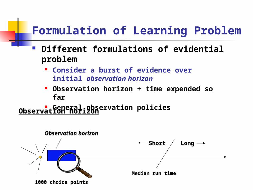
Formulation of Learning Problem Different formulations of evidential problem

Consider a burst of evidence over initial observation horizon

Observation horizon + time expended so far General observation policies

LongLongShortShort

Observation horizonObservation horizon

Median run timeMedian run time

1000 choice points1000 choice points

Observation horizonObservation horizon

Observation horizon + Time expendedObservation horizon + Time expended

Formulation of Learning Problem Different formulations of evidential problem

Consider a burst of evidence over initial observation horizon

Observation horizon + time expended so far General observation policies

LongLongShortShort

Observation horizonObservation horizon

Median run timeMedian run time

1000 choice points1000 choice points tt11 tt22 tt33

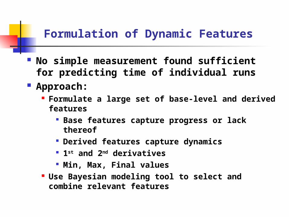
Formulation of Dynamic Features

No simple measurement found sufficient for predicting time of individual runs

Approach: Formulate a large set of base-level and derived features

Base features capture progress or lack thereof Derived features capture dynamics 1st and 2nd derivatives Min, Max, Final values

Use Bayesian modeling tool to select and combine relevant features

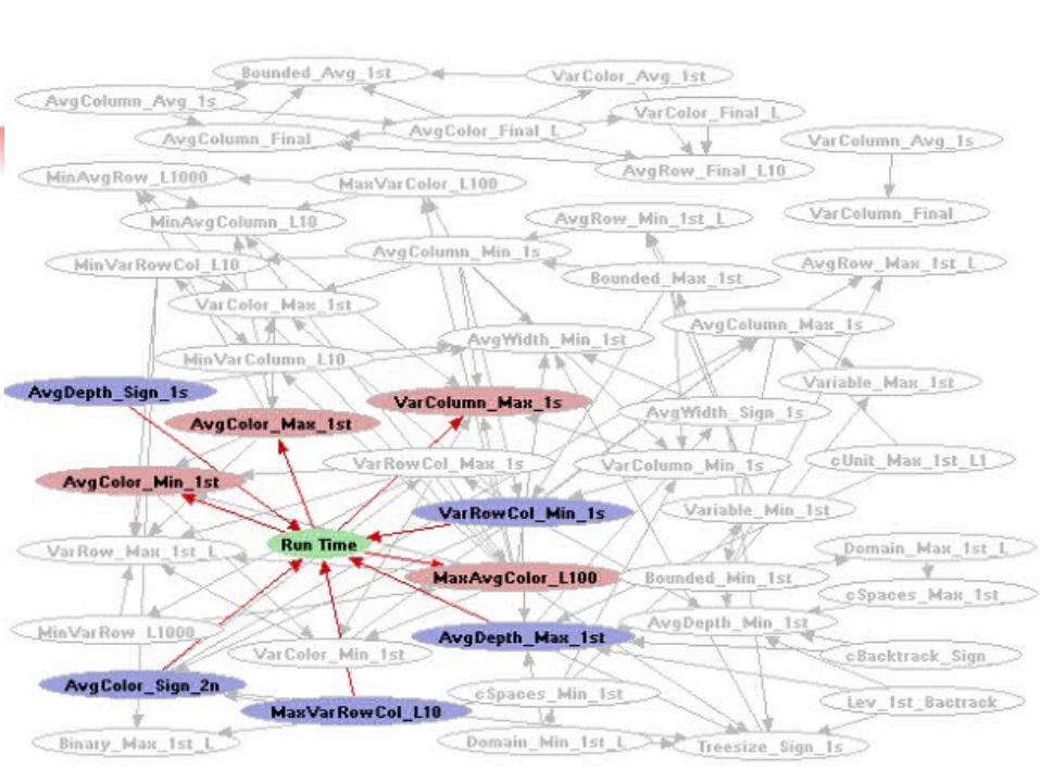
CSP: 18 basic features, summarized by 135 variables # backtracks depth of search tree avg. domain size of unbound CSP variables variance in distribution of unbound CSP variables

Satz: 25 basic features, summarized by 127 variables # unbound variables # variables set positively Size of search tree Effectiveness of unit propagation and lookahead Total # of truth assignments ruled out Degree interaction between binary clauses,

Dynamic Features

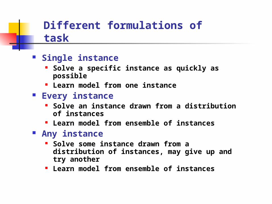
Single instance Solve a specific instance as quickly as possible Learn model from one instance

Every instance Solve an instance drawn from a distribution of

instances Learn model from ensemble of instances

Any instance Solve some instance drawn from a distribution of

instances, may give up and try another Learn model from ensemble of instances

Different formulations of task

Sample Results: CSP-QWH-Single

QWH order 34, 380 unassigned Observation horizon without time Training: Solve 4000 times with random

Test: Solve 1000 times Learning: Bayesian network model

MS Research tool Structure search with Bayesian information criterion

(Chickering, et al. ) Model evaluation:

Average 81% accurate at classifying run time vs. 50% with just background statistics (range of 98% - 78%)

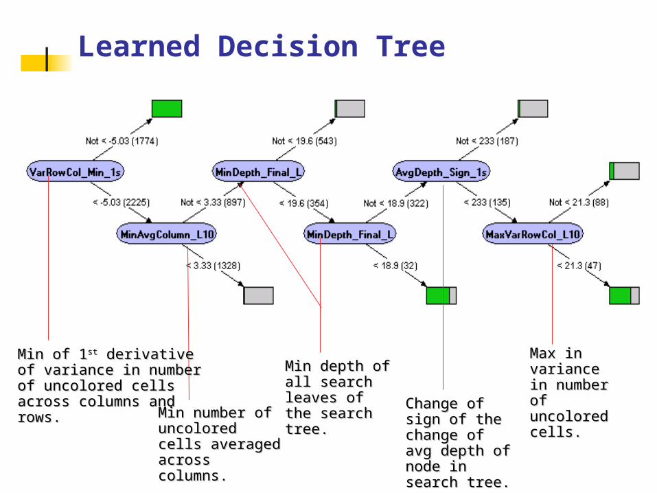
Learned Decision Tree

Min of 1Min of 1stst derivative of derivative of variance in number of variance in number of uncolored cells across uncolored cells across columns and rows.columns and rows.

Min number of Min number of uncolored cells uncolored cells averaged across averaged across columns.columns.

Min depth of all Min depth of all search leaves of search leaves of the search tree.the search tree. Change of sign Change of sign

of the change of of the change of avg depth of avg depth of node in search node in search tree. tree.

Max in Max in variance in variance in number of number of uncolored uncolored cells.cells.

Restart Policies

Model can be used to create policies that are better than any policy that only uses run-time distribution

Example:Observe for 1,000 steps

If “run time > median” predicted, restart immediately;

else run until median reached or solution found;

If no solution, restart. E(Rfixed) = 38,000 but E(Rpredict) = 27,000 Can sometimes beat fixed even if

observation horizon > optimal fixed !

Ongoing work

Optimal predictive policies Dynamic features + Run time + Static features Partial information about run time distribution

E.g.: mixture of two or more subclasses of problems Cheap approximations to optimal policies

Myoptic Bayes

Conclusions

Exciting new direction for improving power of search and reasoning algorithms

Many knobs to learn how to twist Noise level, restart policies just a start

Lots of opportunities for cross-disciplinary work Theory Machine learning Experimental AI and OR Reasoning under uncertainty Statistical physics