Learning to Explain: An Information-Theoretic Perspectiveon Model Interpretation

Jianbo Chen 1 2 Le Song 3 4 Martin J. Wainwright 1 5 Michael I. Jordan 1

AbstractWe introduce instancewise feature selection asa methodology for model interpretation. Ourmethod is based on learning a function to ex-tract a subset of features that are most informativefor each given example. This feature selector istrained to maximize the mutual information be-tween selected features and the response variable,where the conditional distribution of the responsevariable given the input is the model to be ex-plained. We develop an efficient variational ap-proximation to the mutual information, and showthe effectiveness of our method on a variety ofsynthetic and real data sets using both quantitativemetrics and human evaluation.

1. IntroductionInterpretability is an extremely important criterion when amachine learning model is applied in areas such as medicine,financial markets, and criminal justice (e.g., see the discus-sion paper by Lipton ((Lipton, 2016)), as well as referencestherein). Many complex models, such as random forests,kernel methods, and deep neural networks, have been devel-oped and employed to optimize prediction accuracy, whichcan compromise their ease of interpretation.

In this paper, we focus on instancewise feature selection as aspecific approach for model interpretation. Given a machinelearning model, instancewise feature selection asks for theimportance score of each feature on the prediction of a giveninstance, and the relative importance of each feature is al-lowed to vary across instances. Thus, the importance scorescan act as an explanation for the specific instance, indicatingwhich features are the key for the model to make its predic-tion on that instance. A related concept in machine learning

1University of California, Berkeley 2Work done partially duringan internship at Ant Financial 3Georgia Institute of Technology4Ant Financial 5The Voleon Group. Correspondence to: JianboChen <jianbochen@berkeley.edu>.

Proceedings of the 35 th International Conference on MachineLearning, Stockholm, Sweden, PMLR 80, 2018. Copyright 2018by the author(s).

is feature selection, which selects a subset of features thatare useful to build a good predictor for a specified responsevariable (Guyon & Elisseeff, 2003). While feature selectionproduces a global importance of features with respect to theentire labeled data set, instancewise feature selection mea-sures feature importance locally for each instance labeledby the model.

Existing work on interpreting models approach the prob-lem from two directions. The first line of work computesthe gradient of the output of the correct class with respectto the input vector for the given model, and uses it as asaliency map for masking the input (Simonyan et al., 2013;Springenberg et al., 2014). The gradient is computed usinga Parzen window approximation of the original classifierif the original one is not available (Baehrens et al., 2010).Another line of research approximates the model to be in-terpreted via a locally additive model in order to explainthe difference between the model output and some “refer-ence” output in terms of the difference between the inputand some “reference” input (Bach et al., 2015; Kindermanset al., 2016; Ribeiro et al., 2016; Lundberg & Lee, 2017;Shrikumar et al., 2017; Sundararajan et al., 2017). Ribeiroet al. (2016) proposed the LIME, methods which randomlydraws instances from a density centered at the sample tobe explained, and fits a sparse linear model to predict themodel outputs for these instances. Shrikumar et al. (2017)presented DeepLIFT, a method designed specifically forneural networks, which decomposes the output of a neuralnetwork on a specific input by backpropagating the contri-bution back to every feature of the input. Lundberg & Lee(2017) used Shapley values to quantify the importance offeatures of a given input, and proposed a sampling basedmethod “kernel SHAP” for approximating Shapley values.(Sundararajan et al., 2017) proposed Integrated Gradients(IG), which constructs the additive model by cumulating thegradients along the line between the input and the referencepoint. Essentially, the two directions both approximate themodel locally via an additive model, with different defini-tions of locality. While the first one considers infinitesimalregions on the decision surface and takes the first-order termin the Taylor expansion as the additive model, the secondone considers the finite difference between an input vectorand a reference vector.

Learning to Explain: An Information-Theoretic Perspective on Model Interpretation

Training Efficiency Additive Model-agnosticParzen (Baehrens et al., 2010) Yes High Yes Yes

Salient map (Simonyan et al., 2013) No High Yes NoLRP (Bach et al., 2015) No High Yes No

LIME (Ribeiro et al., 2016) No Low Yes YesKernel SHAP (Lundberg & Lee, 2017) No Low Yes Yes

DeepLIFT (Shrikumar et al., 2017) No High Yes NoIG (Sundararajan et al., 2017) No Medium Yes No

L2X Yes High No Yes

Table 1. Summary of the properties of different methods. “Train-ing” indicates whether a method requires training on an unlabeleddata set. “Efficiency” qualitatively evaluates the computationaltime during single interpretation. “Additive” indicates whether amethod is locally additive. “Model-agnostic” indicates whether amethod is generic to black-box models.

In this paper, our approach to instancewise feature selectionis via mutual information, a conceptually different perspec-tive from existing approaches. We define an “explainer,” orinstancewise feature selector, as a model which returns adistribution over the subset of features given the input vector.For a given instance, an ideal explainer should assign thehighest probability to the subset of features that are most in-formative for the associated model response. This motivatesus to maximize the mutual information between the selectedsubset of features and the response variable with respectto the instancewise feature selector. Direct estimation ofmutual information and discrete feature subset sampling areintractable; accordingly, we derive a tractable method byfirst applying a variational lower bound for mutual informa-tion, and then developing a continuous reparametrization ofthe sampling distribution.

At a high level, the primary differences between our ap-proach and past work are the following. First, our frame-work globally learns a local explainer, and therefore takesthe distribution of inputs into consideration. Second, ourframework removes the constraint of local feature additivityon an explainer. These distinctions enable our framework toyield a more efficient, flexible, and natural approach for in-stancewise feature selection. In summary, our contributionsin this work are as follows (see also Table 1 for systematiccomparisons):

• We propose an information-based framework for in-stancewise feature selection.

• We introduce a learning-based method for instancewisefeature selection, which is both efficient and model-agnostic.

Furthermore, we show that the effectiveness of our methodon a variety of synthetic and real data sets using both quanti-tative metric and human evaluation on Amazon MechanicalTurk.

2. A frameworkWe now lay out the primary ingredients of our general ap-proach. While our framework is generic and can be appliedto both classification and regression models, the currentdiscussion is restricted to classification models. We assume

one has access to the output of a model as a conditionaldistribution, Pm(· | x), of the response variable Y given therealization of the input random variable X = x ∈ Rd.

X XS

S

E

Figure 1. The graphical model of obtaining XS from X .

2.1. Mutual informationOur method is derived from considering the mutual infor-mation between a particular pair of random vectors, so webegin by providing some basic background. Given two ran-dom vectors X and Y , the mutual information I(X;Y ) isa measure of dependence between them; intuitively, it cor-responds to how much knowledge of one random vectorreduces the uncertainty about the other. More precisely, themutual information is given by the Kullback-Leibler diver-gence of the product of marginal distributions of X and Yfrom the joint distribution of X and Y (Cover & Thomas,2012); it takes the form

I(X;Y ) = EX,Y[log

pXY (X,Y )

pX(X)pY (Y )

],

where pXY and pX , pY are the joint and marginal prob-ability densities if X,Y are continuous, or the joint andmarginal probability mass functions if they are discrete. Theexpectation is taken with respect to the joint distribution ofX and Y . One can show the mutual information is nonneg-ative and symmetric in two random variables. The mutualinformation has been a popular criteria in feature selection,where one selects the subset of features that approximatelymaximizes the mutual information between the responsevariable and the selected features (Gao et al., 2016; Penget al., 2005). Here we propose to use mutual information asa criteria for instancewise feature selection.

2.2. How to construct explanationsWe now describe how to construct explanations using mu-tual information. In our specific setting, the pair (X,Y )are characterized by the marginal distribution X ∼ PX(·),and a family of conditional distributions of the form(Y | x) ∼ Pm(· | x). For a given positive integer k, let℘k = {S ⊂ 2d | |S| = k} be the set of all subsets ofsize k. An explainer E of size k is a mapping from thefeature space Rd to the power set ℘k; we allow the map-ping to be randomized, meaning that we can also think ofE as mapping x to a conditional distribution P(S | x) overS ∈ ℘k. Given the chosen subset S = E(x), we use xS todenote the sub-vector formed by the chosen features. Weview the choice of the number of explaining features k as

Learning to Explain: An Information-Theoretic Perspective on Model Interpretation

best left in the hands of the user, but it can also be tuned asa hyper-parameter.

We have thus defined a new random vector XS ∈ Rk; seeFigure 1 for a probabilistic graphical model representing itsconstruction. We formulate instancewise feature selectionas seeking explainer that optimizes the criterion

maxE

I(XS ;Y ) subject to S ∼ E(X). (1)

In words, we aim to maximize the mutual information be-tween the response variable from the model and the selectedfeatures, as a function of the choice of selection rule.

It turns out that a global optimum of Problem (1) has a nat-ural information-theoretic interpretation: it corresponds tothe minimization of the expected length of encoded mes-sage for the model Pm(Y | x) using Pm(Y |xS), where thelatter corresponds to the conditional distribution of Y uponobserving the selected sub-vector. More concretely, we havethe following:

Theorem 1. Letting Em[· | x] denote the expectation overPm(· | x), define

E∗(x) := argminS

Em[log

1

Pm(Y | xS)

∣∣∣ x] . (2)

Then E∗ is a global optimum of Problem (1). Conversely,any global optimum of Problem (1) degenerates to E∗ al-most surely over the marginal distribution PX .

The proof of Theorem 1 is left to the supplementary materi-als. In practice, the above global optimum is obtained onlyif the explanation family E is sufficiently large. In the casewhen Pm(Y |xS) is unknown or computationally expensiveto estimate accurately, we can choose to restrict E to suitablycontrolled families so as to prevent overfitting.

3. Proposed methodA direct solution to Problem (1) is not possible, so that weneed to approach it by a variational approximation. In par-ticular, we derive a lower bound on the mutual information,and we approximate the model conditional distribution Pmby a suitably rich family of functions.

3.1. Obtaining a tractable variational formulationWe now describe the steps taken to obtain a tractable varia-tional formulation.

A variational lower bound: Mutual information betweenXS and Y can be expressed in terms of the conditionaldistribution of Y given XS :

I(XS ;Y ) = E[log

Pm(XS , Y )

P(XS)Pm(Y )

]= E

[log

Pm(Y |XS)

Pm(Y )

]= E

[logPm(Y |XS)

]+ Const.

= EXES|XEY |XS

[logPm(Y |XS)

]+ Const.

For a generic model, it is impossible to compute expecta-tions under the conditional distribution Pm(· | xS). Hencewe introduce a variational family for approximation:

Q : ={Q | Q = {xS → QS(Y |xS), S ∈ ℘k}

}. (3)

Note each member Q of the family Q is a collection ofconditional distributions QS(Y |xS), one for each choiceof k-sized feature subset S. For any Q, an application ofJensen’s inequality yields the lower bound

EY |XS[logPm(Y |XS)] ≥

∫Pm(Y |XS) logQS(Y |XS)

= EY |XS[logQS(Y |XS)],

where equality holds if and only if Pm(Y |XS) andQS(Y |XS) are equal in distribution. We have thus ob-tained a variational lower bound of the mutual informationI(XS ;Y ). Problem (1) can thus be relaxed as maximizingthe variational lower bound, over both the explanation Eand the conditional distribution Q:

maxE,Q

E[logQS(Y | XS)

]such that S ∼ E(X). (4)

For generic choices Q and E , it is still difficult to solve thevariational approximation (4). In order to obtain a tractablemethod, we need to restrict both Q and E to suitable familiesover which it is efficient to perform optimization.

A single neural network for parametrizing Q: Recallthat Q = {QS(· | xS), S ∈ ℘k} is a collection of condi-tional distributions with cardinality |Q| =

(dk

). We assume

X is a continuous random vector, and Pm(Y | x) is contin-uous with respect to x. Then we introduce a single neuralnetwork function gα : Rd × [c]→ [0, 1] for parametrizingQ, where [c] = {0, 1, . . . , c− 1} denotes the set of possibleclasses, and α denotes the learnable parameters. We defineQS(Y |xS) : = gα(xS , Y ), where xS ∈ Rd is transformedfrom x by replacing entries not in S with zeros:

(xS)i =

{xi, i ∈ S,0, i /∈ S.

When X contains discrete features, we embed each discretefeature with a vector, and the vector representing a specificfeature is set to zero simultaneously when the correspondingfeature is not in S.

3.2. Continuous relaxation of subset sampling

Direct estimation of the objective function in equation (4)requires summing over

(dk

)combinations of feature sub-

sets after the variational approximation. Several tricksexist for tackling this issue, like REINFORCE-type Al-gorithms (Williams, 1992), or weighted sum of featuresparametrized by deterministic functions of X . (A similarconcept to the second trick is the “soft attention” struc-ture in vision (Ba et al., 2014) and NLP (Bahdanau et al.,2014) where the weight of each feature is parametrized by

Learning to Explain: An Information-Theoretic Perspective on Model Interpretation

a function of the respective feature itself.) We employ analternative approach generalized from Concrete Relaxation(Gumbel-softmax trick) (Jang et al., 2017; Maddison et al.,2014; 2016), which empirically has a lower variance thanREINFORCE and encourages discreteness (Raffel et al.,2017).

The Gumbel-softmax trick uses the concrete distribution asa continuous differentiable approximation to a categoricaldistribution. In particular, suppose we want to approximate acategorical random variable represented as a one-hot vectorin Rd with category probability p1, p2, . . . , pd. The randomperturbation for each category is independently generatedfrom a Gumbel(0, 1) distribution:

Gi = − log(− log ui), ui ∼ Uniform(0, 1).

We add the random perturbation to the log probability ofeach category and take a temperature-dependent softmaxover the d-dimensional vector:

Ci =exp{(log pi +Gi)/τ}∑dj=1 exp{(log pj +Gj)/τ}

.

The resulting random vector C = (C1, . . . , Cd) is called aConcrete random vector, which we denote by

C ∼ Concrete(log p1, . . . , log pd).

We apply the Gumbel-softmax trick to approximateweighted subset sampling. We would like to sample a sub-set S of k distinct features out of the d dimensions. Thesampling scheme for S can be equivalently viewed as sam-pling a k-hot random vector Z from Dd

k : = {z ∈ {0, 1}d |∑zi = k}, with each entry of z being one if it is in the

selected subset S and being zero otherwise. An importancescore which depends on the input vector is assigned for eachfeature. Concretely, we define wθ : Rd → Rd that maps theinput to a d-dimensional vector, with the ith entry of wθ(X)representing the importance score of the ith feature.

We start with approximating sampling k distinct featuresout of d features by the sampling scheme below: Sam-ple a single feature out of d features independently for ktimes. Discard the overlapping features and keep the rest.Such a scheme samples at most k features, and is easierto approximate by a continuous relaxation. We further ap-proximate the above scheme by independently sampling kindependent Concrete random vectors, and then we definea d-dimensional random vector V that is the elementwisemaximum of C1, C2, . . . , Ck:

Cj ∼ Concrete(wθ(X)) i.i.d. for j = 1, 2, . . . , k,

V = (V1, V2, . . . , Vd), Vi = maxjCji .

The random vector V is then used to approximate the k-hotrandom vector Z during training.

We write V = V (θ, ζ) as V is a function of θ and a collec-tion of auxiliary random variables ζ sampled independently

from the Gumbel distribution. Then we use the elementwiseproduct V (θ, ζ)�X between V andX as an approximationof XS .

3.3. The final objective and its optimization

After having applied the continuous approximation of fea-ture subset sampling, we have reduced Problem (4) to thefollowing:

maxθ,α

EX,Y,ζ[log gα(V (θ, ζ)�X,Y )

], (5)

where gα denotes the neural network used to approximatethe model conditional distribution, and the quantity θ is usedto parametrize the explainer. In the case of classificationwith c classes, we can write

EX,ζ[ c∑y=1

[Pm(y | X) log gα(V (θ, ζ)�X, y)]. (6)

Note that the expectation operator EX,ζ does not depend onthe parameters (α, θ), so that during the training stage, wecan apply stochastic gradient methods to jointly optimizethe pair (α, θ). In each update, we sample a mini-batch ofunlabeled data with their class distributions from the modelto be explained, and the auxiliary random variables ζ, andwe then compute a Monte Carlo estimate of the gradient ofthe objective function (6).

3.4. The explaining stage

During the explaining stage, the learned explainer mapseach sample X to a weight vector wθ(X) of dimension d,each entry representing the importance of the correspondingfeature for the specific sample X . In order to provide a de-terministic explanation for a given sample, we rank featuresaccording to the weight vector, and the k features with thelargest weights are picked as the explaining features.

For each sample, only a single forward pass through the neu-ral network parametrizing the explainer is required to yieldexplanation. Thus our algorithm is much more efficientin the explaining stage compared to other model-agnosticexplainers like LIME or Kernel SHAP which require thou-sands of evaluations of the original model per sample.

4. ExperimentsWe carry out experiments on both synthetic and real datasets. For all experiments, we use RMSprop (Maddison et al.,2016) with the default hyperparameters for optimization.We also fix the step size to be 0.001 across experiments.The temperature for Gumbel-softmax approximation is fixedto be 0.1. Codes for reproducing the key results are avail-able online at https://github.com/Jianbo-Lab/L2X.

Learning to Explain: An Information-Theoretic Perspective on Model Interpretation

TaylorSaliency

DeepLIFT SHAP LIME L2X

101

102

103

Cloc

k tim

e (s

)Clock time for various methods

Orange skinXORNonlinear additiveFeature switching

Figure 2. The clock time (in log scale) of explaining 10, 000 sam-ples for each method. The training time of L2X is shown intranslucent bars.4.1. Synthetic Data

We begin with experiments on four synthetic data sets:

• 2-dimensional XOR as binary classification. The inputvector X is generated from a 10-dimensional standardGaussian. The response variable Y is generated fromP (Y = 1|X) ∝ exp{X1X2}.

• Orange Skin. The input vector X is generated from a 10-dimensional standard Gaussian. The response variable Yis generated from P (Y = 1|X) ∝ exp{

∑4i=1X

2i − 4}.

• Nonlinear additive model. Generate X from a10-dimensional standard Gaussian. The responsevariable Y is generated from P (Y = 1|X) ∝exp{−100 sin(2X1) + 2|X2|+X3 + exp{−X4}}.

• Switch feature. GenerateX1 from a mixture of two Gaus-sians centered at ±3 respectively with equal probability.If X1 is generated from the Gaussian centered at 3, the2−5th dimensions are used to generate Y like the orangeskin model. Otherwise, the 6− 9th dimensions are usedto generate Y from the nonlinear additive model.

The first three data sets are modified from commonly useddata sets in the feature selection literature (Chen et al., 2017).The fourth data set is designed specifically for instancewisefeature selection. Every sample in the first data set has thefirst two dimensions as true features, where each dimensionitself is independent of the response variable Y but thecombination of them has a joint effect on Y . In the seconddata set, the samples with positive labels centered around asphere in a four-dimensional space. The sufficient statisticis formed by an additive model of the first four features. Theresponse variable in the third data set is generated from anonlinear additive model using the first four features. Thelast data set switches important features (roughly) based onthe sign of the first feature. The 1− 5 features are true forsamples with X1 generated from the Gaussian centered at−3, and the 1, 6− 9 features are true otherwise.

We compare our method L2X (for “Learning to Explain”)with several strong existing algorithms for instancewise

feature selection, including Saliency (Simonyan et al., 2013),DeepLIFT (Shrikumar et al., 2017), SHAP (Lundberg &Lee, 2017), LIME (Ribeiro et al., 2016). Saliency refers tothe method that computes the gradient of the selected classwith respect to the input feature and uses the absolute valuesas importance scores. SHAP refers to Kernel SHAP. Thenumber of samples used for explaining each instance forLIME and SHAP is set as default for all experiments. Wealso compare with a method that ranks features by the inputfeature times the gradient of the selected class with respectto the input feature. Shrikumar et al. (2017) showed it isequivalent to LRP (Bach et al., 2015) when activations arepiecewise linear, and used it in Shrikumar et al. (2017) asa strong baseline. We call it “Taylor” as it is the first-orderTaylor approximation of the model.

Our experimental setup is as follows. For each data set, wetrain a neural network model with three hidden dense lay-ers. We can safely assume the neural network has success-fully captured the important features, and ignored noise fea-tures, based on its error rate. Then we use Taylor, Saliency,DeepLIFT, SHAP, LIME, and L2X for instancewise featureselection on the trained neural network models. For L2X,the explainer is a neural network composed of two hiddenlayers. The variational family is composed of three hid-den layers. All layers are linear with dimension 200. Thenumber of desired features k is set to the number of truefeatures.

The underlying true features are known for each sample,and hence the median ranks of selected features for eachsample in a validation data set are reported as a performancemetric, the box plots of which have been plotted in Figure 3.We observe that L2X outperforms all other methods onnonlinear additive and feature switching data sets. On theXOR model, DeepLIFT, SHAP and L2X achieve the bestperformance. On the orange skin model, all algorithms havenear optimal performance, with L2X and LIME achievingthe most stable performance across samples.

We also report the clock time of each method in Figure 2,where all experiments were performed on a single NVidiaTesla k80 GPU, coded in TensorFlow. Across all the fourdata sets, SHAP and LIME are the least efficient as theyrequire multiple evaluations of the model. DeepLIFT, Tay-lor and Saliency requires a backward pass of the model.DeepLIFT is the slowest among the three, probably due tothe fact that backpropagation of gradients for Taylor andSaliency are built-in operations of TensorFlow, while back-propagation in DeepLIFT is implemented with high-leveloperations in TensorFlow. Our method L2X is the mostefficient in the explanation stage as it only requires a for-ward pass of the subset sampler. It is much more efficientcompared to SHAP and LIME even after the training timehas been taken into consideration, when a moderate number

Learning to Explain: An Information-Theoretic Perspective on Model Interpretation

TaylorSaliency

DeepLIFT SHAP LIME L2X

2

4

6

8

10

Med

ian

rank

XOR

TaylorSaliency

DeepLIFT SHAP LIME L2X

2

4

6

8

10

Med

ian

rank

Orange skin

TaylorSaliency

DeepLIFT SHAP LIME L2X

2

4

6

8

10

Med

ian

rank

Nonlinear additive

TaylorSaliency

DeepLIFT SHAP LIME L2X

2

4

6

8

10

Med

ian

rank

Feature switching

Figure 3. The box plots for the median ranks of the influential features by each sample, over 10, 000 samples for each data set. The redline and the dotted blue line on each box is the median and the mean respectively. Lower median ranks are better. The dotted green linesindicate the optimal median rank.

Truth Model Key words

positive positive Ray Liotta and Tom Hulce shine in this sterling example of brotherly love and commitment. Hulce playsDominick, (nicky) a mildly mentally handicapped young man who is putting his 12 minutes younger, twinbrother, Liotta, who plays Eugene, through medical school. It is set in Baltimore and deals with the issuesof sibling rivalry, the unbreakable bond of twins, child abuse and good always winning out over evil. It iscaptivating, and filled with laughter and tears. If you have not yet seen this film, please rent it, I promise,you’ll be amazed at how such a wonderful film could go unnoticed.

negative negative Sorry to go against the flow but I thought this film was unrealistic, boring and way too long. I got tired ofwatching Gena Rowlands long arduous battle with herself and the crisis she was experiencing. Maybe thefilm has some cinematic value or represented an important step for the director but for pure entertainmentvalue. I wish I would have skipped it.

negative positive This movie is chilling reminder of Bollywood being just a parasite of Hollywood. Bollywood also tendsto feed on past blockbusters for furthering its industry. Vidhu Vinod Chopra made this movie with thereasoning that a cocktail mix of deewar and on the waterfront will bring home an oscar. It turned out to berookie mistake. Even the idea of the title is inspired from the Elia Kazan classic. In the original, Brandois shown as raising doves as symbolism of peace. Bollywood must move out of Hollywoods shadow if itneeds to be taken seriously.

positive negative When a small town is threatened by a child killer, a lady police officer goes after him by pretending to behis friend. As she becomes more and more emotionally involved with the murderer her psyche begins totake a beating causing her to lose focus on the job of catching the criminal. Not a film of high voltageexcitement, but solid police work and a good depiction of the faulty mind of a psychotic loser.

Table 2. True labels and labels predicted by the model are in the first two columns. Key words picked by L2X are highlighted in yellow.

of samples (10,000) need to be explained. As the scale ofthe data to be explained increases, the training of L2X ac-counts for a smaller proportion of the over-all time. Thusthe relative efficiency of L2X to other algorithms increaseswith the size of a data set.

4.2. IMDB

The Large Movie Review Dataset (IMDB) is a dataset ofmovie reviews for sentiment classification (Maas et al.,2011). It contains 50, 000 labeled movie reviews, with a

split of 25, 000 for training and 25, 000 for testing. Theaverage document length is 231 words, and 10.7 sentences.We use L2X to study two popular classes of models forsentiment analysis on the IMDB data set.

4.2.1. EXPLAINING A CNN MODEL WITH KEY WORDS

Convolutional neural networks (CNN) have shown excel-lent performance for sentiment analysis (Kim, 2014; Zhang& Wallace, 2015). We use a simple CNN model onKeras (Chollet et al., 2015) for the IMDB data set, which

Learning to Explain: An Information-Theoretic Perspective on Model Interpretation

Truth Predicted Key sentence

positive positive There are few really hilarious films about science fiction but this one will knock your sox off. The leadMartians Jack Nicholson take-off is side-splitting. The plot has a very clever twist that has be seen to beenjoyed. This is a movie with heart and excellent acting by all. Make some popcorn and have a greatevening.

negative negative You get 5 writers together, have each write a different story with a different genre, and then you try tomake one movie out of it. Its action, its adventure, its sci-fi, its western, its a mess. Sorry, but this movieabsolutely stinks. 4.5 is giving it an awefully high rating. That said, its movies like this that make methink I could write movies, and I can barely write.

negative positive This movie is not the same as the 1954 version with Judy garland and James mason, and that is a shamebecause the 1954 version is, in my opinion, much better. I am not denying Barbra Streisand’s talent at all.She is a good actress and brilliant singer. I am not acquainted with Kris Kristofferson’s other work andtherefore I can’t pass judgment on it. However, this movie leaves much to be desired. It is paced slowly, ithas gratuitous nudity and foul language, and can be very difficult to sit through. However, I am not a bigfan of rock music, so its only natural that I would like the judy garland version better. See the 1976 filmwith Barbra and Kris, and judge for yourself.

positive negative The first time you see the second renaissance it may look boring. Look at it at least twice and definitelywatch part 2. it will change your view of the matrix. Are the human people the ones who started the war?Is ai a bad thing?

Table 3. True labels and labels from the model are shown in the first two columns. Key sentences picked by L2X highlighted in yellow.

is composed of a word embedding of dimension 50, a 1-Dconvolutional layer of kernel size 3 with 250 filters, a max-pooling layer and a dense layer of dimension 250 as hiddenlayers. Both the convolutional and the dense layers are fol-lowed by ReLU as nonlinearity, and Dropout (Srivastavaet al., 2014) as regularization. Each review is padded/cut to400 words. The CNN model achieves 90% accuracy on thetest data, close to the state-of-the-art performance (around94%). We would like to find out which k words make themost influence on the decision of the model in a specificreview. The number of key words is fixed to be k = 10 forall the experiments.

The explainer of L2X is composed of a global componentand a local component (See Figure 2 in Yang et al. (2018)).The input is initially fed into a common embedding layerfollowed by a convolutional layer with 100 filters. Thenthe local component processes the common output usingtwo convolutional layers with 50 filters, and the global com-ponent processes the common output using a max-poolinglayer followed by a 100-dimensional dense layer. Then weconcatenate the global and local outputs corresponding toeach feature, and process them through one convolutionallayer with 50 filters, followed by a Dropout layer (Srivastavaet al., 2014). Finally a convolutional network with kernelsize 1 is used to yield the output. All previous convolutionallayers are of kernel size 3, and ReLU is used as nonlinearity.The variational family is composed of an word embeddinglayer of the same size, followed by an average pooling anda 250-dimensional dense layer. Each entry of the outputvector V from the explainer is multiplied with the embed-ding of the respective word in the variational family. We useboth automatic metrics and human annotators to validatethe effectiveness of L2X.

Post-hoc accuracy. We introduce post-hoc accuracy forquantitatively validating the effectiveness of our method.

Each model explainer outputs a subset of features XS foreach specific sample X . We use Pm(y | XS) to approx-imate Pm(y | XS). That is, we feed in the sample X tothe model with unselected words masked by zero paddings.Then we compute the accuracy of using Pm(y | XS) topredict samples in the test data set labeled by Pm(y | X),which we call post-hoc accuracy as it is computed afterinstancewise feature selection.

Human accuracy. When designing human experiments,we assume that the key words convey an attitude toward amovie, and can thus be used by a human to infer the reviewsentiment. This assumption has been partially validatedgiven the aligned outcomes provided by post-hoc accuracyand by human judges, because the alignment implies theconsistency between the sentiment judgement based on se-lected words from the original model and that from humans.Based on this assumption, we ask humans on Amazon Me-chanical Turk (AMT) to infer the sentiment of a reviewgiven the ten key words selected by each explainer. Thewords adjacent to each other, like “not good at all,” keeptheir adjacency on the AMT interface if they are selectedsimultaneously. The reviews from different explainers havebeen mixed randomly, and the final sentiment of each reviewis averaged over the results of multiple human annotators.We measure whether the labels from human based on se-lected words align with the labels provided by the model,in terms of the average accuracy over 500 reviews in thetest data set. Some reviews are labeled as “neutral” basedon selected words, which is because the selected key wordsdo not contain sentiment, or the selected key words containcomparable numbers of positive and negative words. Thusthese reviews are neither put in the positive nor in the nega-tive class when we compute accuracy. We call this metrichuman accuracy.

The result is reported in Table 4. We observe that the model

Learning to Explain: An Information-Theoretic Perspective on Model Interpretation

prediction based on only ten words selected by L2X alignwith the original prediction for over 90% of the data. The hu-man judgement given ten words also aligns with the modelprediction for 84.4% of the data. The human accuracy iseven higher than that based on the original review, which is83.3% (Yang et al., 2018). This indicates the selected wordsby L2X can serve as key words for human to understand themodel behavior. Table 2 shows the results of our model onfour examples.

4.2.2. EXPLAINING HIERARCHICAL LSTM

Another competitive class of models in sentiment analysisuses hierarchical LSTM (Hochreiter & Schmidhuber, 1997;Li et al., 2015). We build a simple hierarchical LSTM byputting one layer of LSTM on top of word embeddings,which yields a representation vector for each sentence, andthen using another LSTM to encoder all sentence vectors.The output representation vector by the second LSTM ispassed to the class distribution via a linear layer. Boththe two LSTMs and the word embedding are of dimension100. The word embedding is pretrained on a large cor-pus (Mikolov et al., 2013). Each review is padded to contain15 sentences. The hierarchical LSTM model gets around90% accuracy on the test data. We take each sentence as asingle feature group, and study which sentence is the mostimportant in each review for the model.

The explainer of L2X is composed of a 100-dimensionalword embedding followed by a convolutional layer and amax pooling layer to encode each sentence. The encodedsentence vectors are fed through three convolutional layersand a dense layer to get sampling weights for each sentence.The variational family also encodes each sentence with aconvolutional layer and a max pooling layer. The encodingvectors are weighted by the output of the subset sampler,and passed through an average pooling layer and a denselayer to the class probability. All convolutional layers are offilter size 150 and kernel size 3. In this setting, L2X can beinterpreted as a hard attention model (Xu et al., 2015) thatemploys the Gumbel-softmax trick.

Comparison is carried out with the same metrics. For humanaccuracy, one selected sentence for each review is shownto human annotators. The other experimental setups arekept the same as above. We observe that post-hoc accu-racy reaches 84.4% with one sentence selected by L2X, andhuman judgements using one sentence align with the origi-nal model prediction for 77.4% of data. Table 3 shows theexplanations from our model on four examples.

4.3. MNIST

The MNIST data set contains 28×28 images of handwrittendigits (LeCun et al., 1998). We form a subset of the MNISTdata set by choosing images of digits 3 and 8, with 11, 982

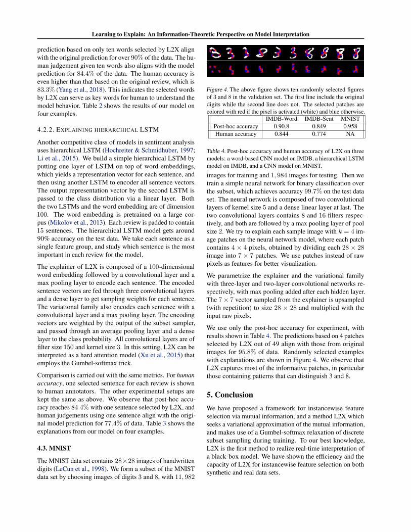
Figure 4. The above figure shows ten randomly selected figuresof 3 and 8 in the validation set. The first line include the originaldigits while the second line does not. The selected patches arecolored with red if the pixel is activated (white) and blue otherwise.

IMDB-Word IMDB-Sent MNISTPost-hoc accuracy 0.90.8 0.849 0.958Human accuracy 0.844 0.774 NA

Table 4. Post-hoc accuracy and human accuracy of L2X on threemodels: a word-based CNN model on IMDB, a hierarchical LSTMmodel on IMDB, and a CNN model on MNIST.

images for training and 1, 984 images for testing. Then wetrain a simple neural network for binary classification overthe subset, which achieves accuracy 99.7% on the test dataset. The neural network is composed of two convolutionallayers of kernel size 5 and a dense linear layer at last. Thetwo convolutional layers contains 8 and 16 filters respec-tively, and both are followed by a max pooling layer of poolsize 2. We try to explain each sample image with k = 4 im-age patches on the neural network model, where each patchcontains 4 × 4 pixels, obtained by dividing each 28 × 28image into 7 × 7 patches. We use patches instead of rawpixels as features for better visualization.

We parametrize the explainer and the variational familywith three-layer and two-layer convolutional networks re-spectively, with max pooling added after each hidden layer.The 7× 7 vector sampled from the explainer is upsampled(with repetition) to size 28 × 28 and multiplied with theinput raw pixels.

We use only the post-hoc accuracy for experiment, withresults shown in Table 4. The predictions based on 4 patchesselected by L2X out of 49 align with those from originalimages for 95.8% of data. Randomly selected exampleswith explanations are shown in Figure 4. We observe thatL2X captures most of the informative patches, in particularthose containing patterns that can distinguish 3 and 8.

5. ConclusionWe have proposed a framework for instancewise featureselection via mutual information, and a method L2X whichseeks a variational approximation of the mutual information,and makes use of a Gumbel-softmax relaxation of discretesubset sampling during training. To our best knowledge,L2X is the first method to realize real-time interpretation ofa black-box model. We have shown the efficiency and thecapacity of L2X for instancewise feature selection on bothsynthetic and real data sets.

Learning to Explain: An Information-Theoretic Perspective on Model Interpretation

AcknowledgementsL.S. was also supported in part by NSF IIS-1218749, NIHBIGDATA 1R01GM108341, NSF CAREER IIS-1350983,NSF IIS-1639792 EAGER, NSF CNS-1704701, ONRN00014-15-1-2340, Intel ISTC, NVIDIA and AmazonAWS. We thank Nilesh Tripuraneni for comments aboutthe Gumbel trick.

ReferencesBa, J., Mnih, V., and Kavukcuoglu, K. Multiple ob-

ject recognition with visual attention. arXiv preprintarXiv:1412.7755, 2014.

Bach, S., Binder, A., Montavon, G., Klauschen, F., Muller,K.-R., and Samek, W. On pixel-wise explanations fornon-linear classifier decisions by layer-wise relevancepropagation. PloS one, 10(7):e0130140, 2015.

Baehrens, D., Schroeter, T., Harmeling, S., Kawanabe, M.,Hansen, K., and MAzller, K.-R. How to explain individ-ual classification decisions. Journal of Machine LearningResearch, 11(Jun):1803–1831, 2010.

Bahdanau, D., Cho, K., and Bengio, Y. Neural machinetranslation by jointly learning to align and translate. arXive-prints, abs/1409.0473, September 2014.

Chen, J., Stern, M., Wainwright, M. J., and Jordan, M. I.Kernel feature selection via conditional covariance mini-mization. In Advances in Neural Information ProcessingSystems 30, pp. 6949–6958. 2017.

Chollet, F. et al. Keras. https://github.com/keras-team/keras, 2015.

Cover, T. M. and Thomas, J. A. Elements of informationtheory. John Wiley & Sons, 2012.

Gao, S., Ver Steeg, G., and Galstyan, A. Variational infor-mation maximization for feature selection. In Advancesin Neural Information Processing Systems, pp. 487–495,2016.

Guyon, I. and Elisseeff, A. An introduction to variable andfeature selection. Journal of machine learning research,3(Mar):1157–1182, 2003.

Hochreiter, S. and Schmidhuber, J. Long short-term memory.Neural computation, 9(8):1735–1780, 1997.

Jang, E., Gu, S., and Poole, B. Categorical reparameteriza-tion with gumbel-softmax. stat, 1050:1, 2017.

Kim, Y. Convolutional neural networks for sentence classi-fication. arXiv preprint arXiv:1408.5882, 2014.

Kindermans, P.-J., Schutt, K., Muller, K.-R., and Dahne,S. Investigating the influence of noise and distractorson the interpretation of neural networks. arXiv preprintarXiv:1611.07270, 2016.

LeCun, Y., Bottou, L., Bengio, Y., and Haffner, P. Gradient-based learning applied to document recognition. Proceed-ings of the IEEE, 86(11):2278–2324, 1998.

Li, J., Luong, M.-T., and Jurafsky, D. A hierarchical neu-ral autoencoder for paragraphs and documents. arXivpreprint arXiv:1506.01057, 2015.

Lipton, Z. C. The mythos of model interpretability. arXivpreprint arXiv:1606.03490, 2016.

Lundberg, S. M. and Lee, S.-I. A unified approach to inter-preting model predictions. pp. 4768–4777, 2017.

Maas, A. L., Daly, R. E., Pham, P. T., Huang, D., Ng, A. Y.,and Potts, C. Learning word vectors for sentiment anal-ysis. In Proceedings of the 49th Annual Meeting of theAssociation for Computational Linguistics: Human Lan-guage Technologies-Volume 1, pp. 142–150. Associationfor Computational Linguistics, 2011.

Maddison, C. J., Tarlow, D., and Minka, T. A* sampling. InAdvances in Neural Information Processing Systems, pp.3086–3094, 2014.

Maddison, C. J., Mnih, A., and Teh, Y. W. The concretedistribution: A continuous relaxation of discrete randomvariables. arXiv preprint arXiv:1611.00712, 2016.

Mikolov, T., Sutskever, I., Chen, K., Corrado, G. S., andDean, J. Distributed representations of words and phrasesand their compositionality. In Advances in neural infor-mation processing systems, pp. 3111–3119, 2013.

Peng, H., Long, F., and Ding, C. Feature selection basedon mutual information criteria of max-dependency, max-relevance, and min-redundancy. IEEE Transactions onpattern analysis and machine intelligence, 27(8):1226–1238, 2005.

Raffel, C., Luong, T., Liu, P. J., Weiss, R. J., and Eck, D.Online and linear-time attention by enforcing monotonicalignments. arXiv preprint arXiv:1704.00784, 2017.

Ribeiro, M. T., Singh, S., and Guestrin, C. Why should itrust you?: Explaining the predictions of any classifier.In Proceedings of the 22nd ACM SIGKDD InternationalConference on Knowledge Discovery and Data Mining,pp. 1135–1144. ACM, 2016.

Shrikumar, A., Greenside, P., and Kundaje, A. Learningimportant features through propagating activation differ-ences. In ICML, volume 70 of Proceedings of Machine

Learning to Explain: An Information-Theoretic Perspective on Model Interpretation

Learning Research, pp. 3145–3153. PMLR, 06–11 Aug2017.

Simonyan, K., Vedaldi, A., and Zisserman, A. Deep in-side convolutional networks: Visualising image clas-sification models and saliency maps. arXiv preprintarXiv:1312.6034, 2013.

Springenberg, J. T., Dosovitskiy, A., Brox, T., and Ried-miller, M. Striving for simplicity: The all convolutionalnet. arXiv preprint arXiv:1412.6806, 2014.

Srivastava, N., Hinton, G., Krizhevsky, A., Sutskever, I.,and Salakhutdinov, R. Dropout: A simple way to preventneural networks from overfitting. The Journal of MachineLearning Research, 15(1):1929–1958, 2014.

Sundararajan, M., Taly, A., and Yan, Q. Axiomatic attribu-tion for deep networks. In International Conference onMachine Learning, pp. 3319–3328, 2017.

Williams, R. J. Simple statistical gradient-following algo-rithms for connectionist reinforcement learning. Machinelearning, 8(3-4):229–256, 1992.

Xu, K., Ba, J., Kiros, R., Cho, K., Courville, A., Salakhudi-nov, R., Zemel, R., and Bengio, Y. Show, attend and tell:Neural image caption generation with visual attention.In International Conference on Machine Learning, pp.2048–2057, 2015.

Yang, P., Chen, J., Hsieh, C.-J., Wang, J.-L., and Jordan,M. I. Greedy attack and gumbel attack: Generatingadversarial examples for discrete data. arXiv preprintarXiv:1805.12316, 2018.

Zhang, Y. and Wallace, B. A sensitivity analysis of (andpractitioners’ guide to) convolutional neural networks forsentence classification. arXiv preprint arXiv:1510.03820,2015.