Learning Terrain Dynamics: A Gaussian Process Modeling …

This article has been accepted for inclusion in a future issue of this journal. Content is final as presented, with the exception of pagination.

IEEE TRANSACTIONS ON CONTROL SYSTEMS TECHNOLOGY 1

Learning Terrain Dynamics: A Gaussian ProcessModeling and Optimal Control AdaptationFramework Applied to Robotic Jumping

Alexander H. Chang , Member, IEEE, Christian M. Hubicki , Member, IEEE, Jeffrey J. Aguilar ,

Daniel I. Goldman , Aaron D. Ames , Senior Member, IEEE, and Patricio A. Vela , Member, IEEE

Abstract— The complex dynamics characterizing deformableterrain presents significant impediments toward the real-worldviability of locomotive robotics, particularly for legged machines.We explore vertical, robotic jumping as a model task forlegged locomotion on presumed-uncharacterized, nonrigid ter-rain. By integrating Gaussian process (GP)-based regression andevaluation to estimate ground reaction forces as a function of thestate, a 1-D jumper acquires the capability to learn forcing pro-files exerted by its environment in tandem with achieving its con-trol objective. The GP-based dynamical model initially assumes abaseline rigid, noncompliant surface. As part of an iterative pro-cedure, the optimizer employing this model generates an optimalcontrol strategy to achieve a target jump height. Experiential datarecovered from execution on the true surface model are appliedto train the GP, in turn, providing the optimizer a more richlyinformed dynamical model of the environment. The iterativecontrol-learning procedure was rigorously evaluated in experi-ment, over different surface types, whereby a robotic hopperwas challenged to jump to several different target heights. Eachtask was achieved within ten attempts, over which the terrain’sdynamics were learned. With each iteration, GP predictions ofground forcing became incrementally refined, rapidly matchingexperimental force measurements. The few-iteration convergencedemonstrates a fundamental capacity to both estimate and adaptto unknown terrain dynamics in application-realistic time scales,all with control tools amenable to robotic legged locomotion.

Index Terms— Gaussian process (GP), learning, optimalcontrol, robotic jumping, terrain dynamics.

Manuscript received November 30, 2019; revised March 21, 2020; acceptedJuly 1, 2020. Manuscript received in final form July 13, 2020. This work wassupported by NSF under Grant CPS#1544857. Recommended by AssociateEditor A. Chakrabortty. (Corresponding author: Alexander H. Chang.)

Alexander H. Chang and Patricio A. Vela are with the Institute forRobotics and Intelligent Machines, Georgia Institute of Technology,Atlanta, GA 30332 USA (e-mail: [email protected];[email protected]).

Christian M. Hubicki is with the Department of Mechanical Engi-neering, Florida A&M University–Florida State University, Tallahassee,FL 32310 USA (e-mail: [email protected]).

Jeffrey J. Aguilar and Daniel I. Goldman are with the School ofPhysics, Georgia Institute of Technology, Atlanta, GA 30332 USA (e-mail:[email protected]; [email protected]).

Aaron D. Ames is with the Department of Mechanical and Civil Engineer-ing, California Institute of Technology, Pasadena, CA 91125 USA (e-mail:[email protected]).

Color versions of one or more of the figures in this article are availableonline at http://ieeexplore.ieee.org.

Digital Object Identifier 10.1109/TCST.2020.3009636

I. INTRODUCTION

ENGINEERED mechanical systems are well character-ized through a combination of known design, machining

to precise tolerances, and the use of system identificationtools. Consequently, optimal control formulations for engi-neered systems have demonstrated the ability to provideexcellent performance for even complex systems, such aslegged locomotion [1]–[3]. However, when the underlyingdynamics of the controlled system rely on external factorsthat must be approximated based on empirical models or aresimply unknown, employing optimal control methods leadsto degraded performance. A mismatch between the presumedmodel dynamics and the actual dynamics may prevent thesatisfaction of critical performance outcomes specified withinthe optimal control formulation. As robotics researchers striveto create more complex robotic systems that exploit hard-to-model physical properties, we can expect optimal controlmethods to break down. Such robotic applications prone tomismatch between the theoretical equations and the actualexperience of the mechanical system include legged movementover unknown ground substrates [4], flapping flight [5], [6],and aquatic swimming [7]–[10]. This particular work focuseson vertical, robotic hopping, as a preliminary model taskfor legged locomotion, where terrain dynamics that drivelocomotion are presumed to be poorly modeled or unknown.

A. Review of Related Work

1) Locomotion on Soft Terrain: Control approachesaddressing legged locomotion over soft terrain often relegatesurface deformation effects to uncertainty terms in the con-troller or presume simplifying, closed-form approximations ofthe terrain model (e.g., spring damper) [11]–[14]. Strategiesaccommodating terrain variation may then apply sensor-drivenswitching between terrain-tuned controllers to achieve taskobjectives [15]. These approaches, however, are not wellsuited to achieving high-performance control objectives whenthe underlying terrain is arbitrarily soft or exhibits complexnonlinear behavior.

Prior work regarding robotic jumping on soft ground gran-ular media (GM) alternatively employed optimal trajectorysynthesis, in conjunction with an empirically tuned model of

1063-6536 © 2020 IEEE. Personal use is permitted, but republication/redistribution requires IEEE permission.See https://www.ieee.org/publications/rights/index.html for more information.

Authorized licensed use limited to: Georgia Institute of Technology. Downloaded on November 10,2020 at 03:25:57 UTC from IEEE Xplore. Restrictions apply.

https://orcid.org/0000-0001-9036-100X

https://orcid.org/0000-0003-0848-3177

https://orcid.org/0000-0002-6888-7002

https://orcid.org/0000-0002-2092-3772

https://orcid.org/0000-0003-3055-3215

https://orcid.org/0000-0002-6954-9857


2 IEEE TRANSACTIONS ON CONTROL SYSTEMS TECHNOLOGY

terrain forcing, to achieve precise control objectives [4].As generalized, terradynamic models do not exist (in contrastto fluid systems, for example, which can be modeled gener-ally via Navier–Stokes equations), we relied on meticulouslyderived and experimentally validated models for the GM[16], [17] and applied system identification to the actuator.We demonstrated that distinct ground substrates might lead todiverging optimal control signals for identical control objec-tives [4]; variation of even the GM ground model parameterswill influence different control solutions to accomplish thesame task [16]. Although control strategies may be com-puted in cases where terrain parameters are known a priori,in practice, a robot likely lacks the ability and opportunityto methodically characterize terrain properties prior to taskexecution. Manual effort to do so precludes adaptive use byautonomously operating systems, such as bipedal robots.

Given that the control synthesis must conform to the actualdynamics experienced by the mechanical system, a means torapidly estimate (or learn) online the unknown forcing functiondue to foot–ground interaction is essential to high-performanceoperation.

2) Kernel Machines in Robotics: Kernel machines andradial basis function networks for function approximation areoften applied to control and robotics problems due to theiruniversal approximation capabilities. Though computationallycomplex to implement in the case of online, data-drivenoperation, modifications to the baseline learning methodsprovide online, real-time implementable algorithms [18]–[20].Gaussian processes (GPs), in particular, have received atten-tion in the area of reinforcement learning (RL) [21], [22],where their inclusion expedites the learning process by regress-ing on the unknown model dynamics. RL approaches havebeen combined with optimal control methods to jointly learnthe model dynamics and identify the optimal control policyto apply [23]. A benefit of GPs, in this context, is the abilityto generate random draws from a function space [24] withinthe context of stochastic optimal control. The combinationof efficient GP learning and sample synthesis methods withstochastic optimal control leads to compelling RL strategies[25], [26]. Importantly, these approaches are experiential,data-driven learning methods. Due to the lack of model infor-mation, however, they involve offline training prior to deploy-ment. If deployed online with no prior knowledge, learningtypically involves on the order of hundreds or more examplesdue to the tension between exploration and exploitation.

3) Kernel Machines and Adaptive Control: From a morecontrols oriented perspective, actor-critic networks with expe-rience replay methods have been used to learn optimalpolicies [27]. These offline-learned-then-online-implementedmethods have proven stability and learning properties.Likewise, a method arising from the model referenceneuro-adaptive control literature, known as concurrent learn-ing, can also learn online and has proven stability and learningproperties [28], [29]. Here, proven learning properties meansthat persistent excitation is shown to hold for the kernelmachine regressor dynamics so that the regression variablesof the kernel machines are known to converge exponentiallyfast. Subsequent efforts created online learning methods using

data-driven kernel machine methods that started with nothingand built the model from scratch [30], [31] much like the afore-mentioned RL methods. To achieve online implementation,data curation and sparsification methods were applied [32],where the data curation was informed by the control task andapproximation needs. The method requires a preexisting base-line controller to preserve stability and learning guarantees.

4) Gaussian Process Regression: GP-based regression isone strategy applied to learn uncertainty online. Its utilityin modeling uncertain dynamical elements, stemming fromcomplex robot-terrain interactions, has found application indifferent classes of mobile platforms [33], [34].

GPs applied to learn substrate forcing, in the context ofjumping on a particular simulated GM model, previouslysuggested that online learning would occur rapidly [35].As opposed to learning the dynamics of the entire systemfrom scratch, online learning targeted the unknown externalforcing component. This data-driven approach facilitated theincremental accumulation of knowledge, ultimately permit-ting estimation of the uncertain element driving the system’sdynamics and follow-on model-based optimal control. Theunderlying strategy of targeted learning of unknown dynam-ical quantities was demonstrably practical while being moredimensionally tractable than learning the system dynamics intheir entirety. The nonparametric nature of a GP frees it fromany a priori structural presumptions; we show its applicationas a regression element, in this particular work, provides theflexibility to learn complex dynamical profiles associated withvarious categorically distinct terrain.

B. Target Problem and Contribution

1) Robotic Jumping, a Model Task: Jumping frequentlyfunctions as a model task for legged locomotion as it encom-passes similar mathematical (and physical) challenges. Akin tobipedal running, it requires changes in contact modes (hybridsystem dynamics) and control through periods of underactu-ation (flight phases). The control-learning approach [35] pre-sented here uses optimal control methods for hybrid systems,similar to those at the core of many model-based legged con-trol techniques [2], [36]. The particular application we exploreentails learning of presumed-unknown terrain dynamics thatinfluence vertical, robotic jumping outcomes. The strategy,however, potentially extends to more complex, higher degreeof freedom (DoF) legged systems as well [37], where controlfeasibility continues to be impacted by modeling uncertaintyassociated with complex and unknown robot-terrain interac-tions. Ground forcing, in this context, must be learned quicklywith respect to several DoFs describing robot-terrain motion,in lieu of just vertical motion. Safety measures guardingagainst mechanical instability may guide exploratory controland learning of unmodeled quantities [38], [39]. Evaluation inmore deployment-realistic scenarios, where terrain dynamicsmay transition drastically, warrants adoption of supplementalstrategies to manage novel encounters [40], [41].

2) Contribution: We extend a previously proposed GP-based dynamical model of 1-D jumping, accompanied by adeterministic process to iteratively learn an unknown ground



CHANG et al.: LEARNING TERRAIN DYNAMICS: GP MODELING AND OPTIMAL CONTROL ADAPTATION FRAMEWORK 3

Fig. 1. Flowchart illustrating an iterative optimal control-learning framework. With each jump, the algorithm regresses an updated terrain model and thenuses the learned model to generate and execute a new optimal control signal.

forcing profile, all while optimizing control to achieve thedesired objective [35]. Whereas the original work involvedsimulation, the extensions involve experimental validation thatthe strategy will work in practice by showing reproducibleoutcomes on three different classes of terrain.

Well-understood equations of motion are rearranged tohighlight the presumed-unknown terrain forcing and introducea GP-based component that enables learning. Without priorexperiential data, the GP-based model assumes a baselinerigid ground dynamical representation of the terrain. Optimalcontrol generation is driven by this GP-based model, whichinitially conveys an inaccurate dynamical understanding. In aniterative process, as shown in Fig. 1, optimal control signalsare generated and then evaluated on the true ground model.The forcing profile exerted by the terrain substrate is recoveredfrom measured trajectory data; defects with respect to the base-line rigid ground dynamics are applied to train the GP which,in turn, conveys an incrementally more accurate understandingof the environment to the optimizer. Experimental validation ofthis approach was performed on a 1-D, vertical robotic jumper,operating over a variety of categorically distinct surfaces:leveled solid ground, a trampoline surface, and a bed of poppyseeds (a model GM [17]). The robot quickly accomplishedspecified control tasks, each within 10–15 control-learningiterations. Using this model-based data-driven learning andcontrol approach, each terrain model was learned, and spec-ified tasks were completed precisely, while only requiring asmall set of experiential data.

II. SYSTEM DYNAMICS

This section reviews the equations governing 1-D jumping,as applicable to any surface type, rigid or deformable. Theequations are arranged to highlight terrain substrate forcing,Fsub, the unknown quantity in this system.

A. Equations of Motion

The 1-D jumping model, shown in Fig. 2 and presentedin [16], is modeled by three massed bodies: a linear motor,a thrust rod, and a foot. This robot model jumps by apply-ing force between the motor and thrust rod, which can be

Fig. 2. (a) Visualization and labeling of the 1-D (vertical-only) jumpingrobot model. (b) Illustration of the jumping task; the robot must thrust itsmotor mass to jump off the ground and achieve a specified jump height at itsapex.

leveraged to pump energy into the spring-loaded system.Vertical motor actuation drives rod displacement which,in turn, transmits forcing to the foot through the connectingspring (which is mass-less, but modeled with linear viscousdamping). The closed-form system dynamics are

x f = −g + 1

m f[k(α − α) + cα] + 1

m fFsub

α = −[

m f + mr + mm

m f (mr + mm)(k(α − α) + cα) + mm

mr + mmβ

]

− 1

m fFsub (1)

where body masses of the motor, rod, and foot are designatedmm , mr , and m f , respectively. The signals x f , α, and βrepresent the spatial position of the foot center of mass(CoM), position of the rod CoM relative to the foot CoM,and the position of the motor CoM relative to the rod CoM,respectively. β denotes acceleration of the motor relative tothe rod; in the physical platform, this is driven by dynamicsrelated to internal motor feedback tracking [4]. The controlinput will be a synthesized reference motor trajectory, u = β∗,against which β is tracked to arrive at β. For later reference,xr = x f + α denotes spatial position of the thrust rod.




α represents the position of the rod, relative to the foot, whenno external forcing, gravity or otherwise, acts to compressor extend the spring. Fsub denotes substrate reaction forcesacting on the foot and is always directed positively upward.The system state is defined, x = [x f x f α α]T ∈ IR4.

1) Substrate Force, Fsub: Substrate forcing, Fsub, resistsnegative displacement of the foot and is one mechanism bywhich energy is stored in the spring, ultimately enabling thesystem to lift off from the ground. The model of the substrateforce will vary with the substrate type and the relevant phaseof the hybrid system. During the flight phase, the foot haslifted off the surface and substrate forcing no longer acts onthe system, Fsub = 0. During the stance phase, the foot is incontact with the ground, and x f is coincident with the surfaceheight. The substrate forcing Fsub then becomes a positivequantity, modeled according to the material composition ofthe jumping surface.

Specifically, in a rigid ground scenario, x f = 0. Theresultant force due to gravity, the spring, and damping isdirected in the negative, downward direction. Substrate forcingcounteracts all other forces acting on the foot. Values of Fsub

follow from the first equation in (1), in closed-form, as afunction of state:

FSGsub = m f g−k(α − α)−cα (2)

where superscript SG denotes the assumption of solid, unde-formable ground.

When the ground is no longer rigid and is, instead, modeledas a deformable material, then the assumptions used for solidground scenarios no longer hold. Consider GM, a materialcharacterizing a particular example class of deformable sur-faces. The function FGM

sub , denoting substrate forcing exertedon foot by the GM, becomes a complex nonlinear function ofthe hopper state and is dependent upon empirically determinedparameters modeling the material [16]. It may be decomposedas

FGMsub = Fp + Fv (3)

where Fp denotes a quasi-static forcing component dependentupon foot depth, while Fv varies as a function of depth,velocity, and added mass to the foot during GM intrusion.

In general, deformation of the ground substrate may inducea significant change in the dynamics of the 1-D hopper,in contrast to operation on solid ground. Open-loop signalsdesigned for solid ground scenarios but applied on GM, forexample, lead to system trajectories that may diverge greatlyfrom operation on the former. Fig. 3 (left-hand side) showssuch a scenario. An open-loop control signal is designedto achieve a peak jump height of 30 mm (dashed) on asimulated 1-D, robotic hopper operating on level solid ground.On simulated GM (solid), however, the ground yields andx f (red) sinks prior to takeoff. Terrain deformation dissipatesenergy, robbing it from the spring, ultimately leading to alower peak jump height, 7.64 mm, which falls short of thetarget by 74.5%. The nonlinear behavior of this complex,deformable terrain type does not permit the use of simplefeedback mechanisms; we have seen that tunable control signalcharacteristics, such as amplitude, do not necessarily trend

linearly, nor monotonically, with achieved peak jump height onthis surface [4]. Alternative approaches to legged locomotivecontrol over soft terrain have presumed spring-damper-basedmodels of the robot-ground interactions [11], [13], [14], [42].These assumptions, however, remain ill-suited for operationover GM, a class of terrain characterized by its complex,hydrodynamically driven nonlinear behavior.

In the context of this study, each terrain type the leg hopson will have its own unique substrate interaction force profile,which will require learning.

III. ONLINE LEARNING OF EXTERNAL FORCING

This section describes the GP-based online learning process.In particular, it describes how the measured state variables ofthe robot lead to estimates of external ground forcing, throughan inverse dynamics procedure.

A. Gaussian Processes

GPs present a Bayesian approach to function regression andmodeling over potentially high-dimensional domains and inthe presence of a limited set of function evaluations or trainingdata [43]. Given a set of (possibly noisy) evaluations of anunknown function, τ (x) : IRn → IR, a GP represents a priorover functions

Z(x) ∼ GP(m(x), κ) (4)

where Z(x) : IRn → IR represents the function regression,m(x) is the mean function, and κ(x, x′) is a kernel functiondescribing covariance. We choose to employ a squared expo-nential kernel

κ(x, x ′) = exp

(−1

2

(x − x′)T

�(x − x′)) + σdampI,

x, x′ ∈ IRn (5)

which provides a measure of similarity between any two ele-ments, x and x′, in the domain of τ (x), based on �2 proximity.� is a bandwidth parameter influencing the scale, over thedomain, with which the function regression varies, while σdamp

represents variance associated with noise in the training data.The latter may be interpreted as a damping factor to tune foroverfitting in regression outcomes.

In particular, we approximate the unknown function τ (x) bythe model y(x) = μ(x)+ Z(x), where μ(x) captures a globaltrend from the training data. The global trend is representedas a linear combination of a set of basis functions, f (x) ={1 f1(x) f2(x), . . . , fm(x)}T, such that μ(x) = f (x)T,where ∈ IRm captures the linear coefficients. Z(x) denotesa nonstationary GP representing regression over any residualdeviations from μ(x).

The GP-based function approximation is more specificallyrepresented by [44]

y(x) = μ(x) + rT(x)R−1( y − μ(x)) (6)

where x = [x1 x2, . . . , x p]T and y ∈ IRp together comprise aset of p training samples; the evaluation of each element ofx, xi ∈ IRn, by the unknown function has yielded yi = τ (xi).R is the empirical covariance matrix such that Ri, j = κ(xi , x j )and rT(x) = [κ(x, x1) κ(x, x2), . . . , κ(x, x p)]T.




B. Learning Ground Forcing as a Function of State

To construct a learning-enabled dynamical model of 1-Dhopping, we begin with (1). However, ground forcing, Fsub,will instead be formulated as the summation of multiplecomponents, one of which is a GP

Fsub(x) = FSGsub (x) + μ(x) + rT(x)R−1( y − μ(x)) (7)

where again x and y comprise training data; xi ∈ IR4 andyi ∈ IR together comprise a training tuple, identifying a pointin the state space and the corresponding ground force expe-rienced, respectively. For subsequent reference, these tuplescompose the reference training data set, = {(xi , yi) : i ∈ N,i ≤ p}, where p = || designates cardinality of the data set.

FSGsub (x) is defined by (2). When no training data has

been collected, the latter two components of (7) vanish, andthe model reduces to the baseline solid ground assumption.As training data are collected, the latter two terms of (7) modelcomponents of terrain forcing that represent defects from arigid surface environment.

A global linear trend, μ(x) = f (x)T, is extracted fromthe training data, after which residuals from this global trendare modeled by the GP in the final term of (7). To computeμ(x), let f (x) = [1 x f x f α α]T. Then, the correspondinglinear coefficients are computed in closed form from a damped,weighted least-squares fit

= (FT R−1 F + ρμI

)−1(FT R−1�

)(8)

where � = [(y1 − FSGsub (x1), . . . , (y p − FSG

sub (x p))]T. F =[ f (x1) f (x2), . . . , f (x p)]T and p denotes the cardinality ofthe training set [44]. ρμ is a damping parameter influencingthe pseudoinverse of F .

We have applied a weighted least squares fit as alow-complexity approach to extract a coarse global trend,μ(x), for the terrain forcing function being approximated. TheGP then regresses over the function’s residual that remainsafter this underlying trend has been removed.

C. State Smoothing

Ground forcing, Fsub, applied during the course of the hop-per trajectory must be recovered to train the GP-based modelof (7). Any direct sensing of this quantity is assumed absent.Through recovery of the relevant quantities from the firstequation of (1), however, Fsub can be computed. We assumethe state of the system, x = [x f x f α α], is completelyobservable. In particular, however, acceleration associated withthe foot, x f , is not immediately and conveniently accessible.To recover this quantity, measured trajectory data producedby the dynamical system, (1), is subjected to a fixed-lagKalman smoothing process with trivial integrator dynamics.The output of this process is a smoothed state trajectory,xs(t) = [xs

f (t) x sf (t) x s

f (t) αs(t) αs(t) αs(t)]T, providing themissing quantity x s

f . Substrate forcing is then estimated as afunction of the smoothed system state

Fssub(t) = m f g − [

k(αs(t) − α

) + cαs(t)] + m f x s

f (t). (9)

This smoothed trajectory and recovered forcing data isappended to the training data set, = ∪ {(xi , yi )},

where xi = xsi and yi = (Fs

sub)i . Time parameter, t , has beenreplaced by discrete time index, i .

D. Data Curation

GP training incurs matrix inversion costs whose complexityis O(p3) in the worst case. Evaluation cost of the GP-basedregression model, (7), scales linearly with the cardinalityof the training set, e.g., it is O(p). When used within thenumerical optimization method, the cost of gradient evaluationwill naturally scale with the number of terms required to sym-bolically express the GP-based model of Fsub. This scales bythe evaluation cost O(p) for each gradient iteration. To speedup the learning and optimization computations, we incorporatea data sparsification procedure that trains a GP model from asubset of the full data set [31], [32], [45].

An initial data set, = {(xi , yi) : i ∈ N, i ≤ p}, withcardinality p = || is reduced to the subset ⊆ via aniterative procedure. Initially, = ∅. Each iteration then selectsa random element of the set, (xcent, ycent) ∈ , to serve as acenter; all elements falling within its shadow are culled

cull = {(xi , yi) ∈ : ‖xi − xcent‖� < �−2

cull

}. (10)

The threshold �cull determines which elements are to be culledand associated with the center element, (xcent, ycent). Thescaled Euclidean distance ‖·‖� is the weighted �2-norm, withrespect to the GP squared exponential kernel’s bandwidthparameter, �, in (5). The center is appended to the reduceddata set, = ∪ {(xcent, ycent)}, and the reference data setupdated, = \ cull. This procedure repeats until = ∅.

After every hop, when a new set of batch data is to be assim-ilated into the GP model, data sparsification is first applied.Training with the reduced set uses a density-weighted pro-cedure that factors in the removed data [45] when performingthe matrix inversion during GP training. Data accumulates intothe set as needed (based on �cull).

IV. ITERATIVE OPTIMAL CONTROL-LEARNING FRAMEWORK

The dynamics model, force recovery procedure, and learn-ing process contribute to an online, iterative optimal controlsynthesis and learning framework [35]. In a prior imple-mentation of the framework, a cyclic procedure (Fig. 1) togenerate an optimal motion plan, apply it to a robotic hopper,then collect trajectory data and retrain a GP-based model ofground forcing, resulted in optimal control solutions whosepredicted hopper trajectories coincided with simulated realityafter a few control-learning iterations. This section delineatesthe procedure and supporting components.

A. Optimal Jumping Control

This work leverages trajectory optimization methods togenerate an optimal control solution, u = β∗. Using a directcollocation approach, a trajectory optimization problem is tran-scribed into a large-scale nonlinear program (NLP) [46], [47].An NLP formulation allows casting of hard constraints, such asphysical and task constraints, as inequality/equality constraints




rather than as weighting factors within the objective function.Furthermore, direct collocation approaches admit computationof all objectives, constraints, and derivatives thereof in closed-form.

In this work, objectives, constraints, and their respectivederivatives are all exported as closed-form expressions by aMATLAB-based parser [48]; the resulting NLP is solved usingInterior Point OPTimizer (IPOPT) [49], a large-scale interiorpoint solver. We approximate the trajectory using N = 31trapezoidally integrated collocation points for each of thestance and flight phases of this hybrid system (62 total).

The optimal control specification and problem setup followsthat of [4]. We begin by rearranging our system dynamicsinto a typical set of first-order ordinary differential equations(ODEs), x = f (t, x, u(t)), where t , x, and u(t) are time, state,and time-varying control inputs, respectively. Collocationmethods discretize the optimal control problem and then applya numerical optimizer on the discrete set of variables definingthe piecewise state and control trajectories. This includes adiscrete time tape, td

i , where 0 = td0 < td

1 < td2 <. . .< td

N =T d , and state variables, xd

i , and control inputs, udi , where

i ∈ {1, 2, 3, . . . , N − 1}. Variables are duplicated for eachdynamical domain, d ∈ D = {stance, flight}. The variables,xd

i , udi = β∗,d

i , and tdi , are free variables for the optimization

process to determine. In this manner, durations of each dynam-ical domain, T d , are free to be designed as well. A vector of alloptimization variables, w = {xd

i , xdi , ud

i , β∗,di , td

i }, is built fromstates, first-order time derivatives, and control inputs, over alli and d defined. Depending on the motor’s internal controlloop, definition of additional design variables was required toencode the first-order dynamics of integral control terms.

Each discrete point, i , is rendered dynamically consistentwith the next point, i + 1, via “defect” constraints in the NLP,which approximate implicit integration

(xd

i+1 − xdi

) − 1

2

(tdi+1 − td

i

)(xd

i+1 + xdi

) = 0 (11)

xdi − f

(tdi , xd

i , udi

) = 0 (12)

for all i , derived from a trapezoidal integration scheme.The equations of motion f include the GP-based forcingmodel Fsub in symbolic form.

The control task is to achieve a specified “jump height”defined as the difference between the initial rod height, x0

r ,and the rod’s highest point during the jump, x f

r , as shownin Fig. 2(b). Consequently, targeted jumping requires addingan equality constraint x f

r −x0r = h∗ with h∗ equal to the target

jump height.In hardware implementation, the true actuation signal, β,

arises from a low-level trajectory tracking control loop appliedto the linear motor of Fig. 2(a). The closed-loop motordynamics introduce a dynamic response that impacts jump-ing performance. We explicitly account for these trackingdynamics in the optimization by modeling the control loopas part of the system dynamics [4]. In brief, the solution, u,is computed with anticipation, both of how the tracking willperform given the closed-loop dynamics and the saturationlimits of the actuator force, Fm .

The objective function is defined

J(w) =∑d∈D

[td2 − td

1

2J(

xd1 , xd

1 , ud1, β

∗,d1

)

+N−1∑i=2

tdi+1 − td

i−1

2J(

xdi , xd

i , udi , β

∗,di

)

+ tdN − td

N−1

2J(

xdN , xd

N , udN , β∗,d

N

)](13)

where J (·) is the integrand of a continuous-time cost.We defined the objective integrand to be J = β∗,d

i (t)2, whichpenalized actuator velocity as a proxy for energetic cost andalso favored more-easily trackable position trajectories onhardware. One could substitute instantaneous power as theobjective; however, such power minimizing solutions tendto rail actuator forces violently between zero and nonzerovalues. Such “banging” strategies are typically more sensitiveto timing errors in hardware implementation.

The resulting NLP is

w∗ = argminw

J(w) (14)

s.t. wmin ≤ w ≤ wmax (15)

cmin ≤ c(w) ≤ cmax (16)

where c(w) represents the concatenation of all constraintfunctions, including defect constraints (11) and (12) andtask constraints, such as jumping height, actuator limits,workspace/acceleration limits, and so on [4]. The optimizationroutine was tasked to return a locally optimal control trajec-tory. In addition to the other states in w, the optimizationreturns a vector u = β∗ comprising the concatenation ofsequences, β∗,stance

i and β∗,flighti . In implementation, IPOPT

solved the NLP to a tolerance of 10−9, for both feasibilityand duality. All told, the optimal control computations wereperformed given (1) an a priori robot model, (2) an a priorimodel of the motor control loop, and (3) a GP-based modelof the terrain forcing.

B. Iterative Optimal Control and Learning

We apply an iterative control-learning procedure to recovera GP-based dynamical model of the 1-D hopper system,described jointly by (1) and (7). While hopping on an unknownsurface, the forcing profile that surface exerts as a functionof the system state, x, will be simultaneously learned. Priorto any experimental attempts, the reference training data setis empty, = ∅, corresponding to the zero function forany learned components of the unknown forcing model. Eachlearning iteration begins with the hopper at rest on the jumpingsurface. An optimizer then employs the GP-based dynamicalmodel, described by (1) and (7), to generate an optimal controlsignal enabling a target peak jump height to be attained, whileminimizing actuation effort. The control signal is subsequentlyapplied to the 1-D hopper. If the target peak jump height isnot attained using the generated control signal on the surface,trajectory data are collected, smoothed, and substrate forcing,Fs

sub(t), is recovered per (9). The reference training set, ,




Algorithm 1 Iterative Hopper Control and Learning

is augmented with the computed tuples, (xs(t), Fssub(t)), for all

discretely measured t . This training set is limited to trajectoriesand corresponding forces occurring during the stance phase ofthe jump prior to the hopper transitioning to the flight phase.

The reduced training data set, , is extracted from thecumulative reference set, , with cardinality k ≤ p. It isused to update the GP-based model of substrate forcing.First, the deviation of Fsub(x) from the equivalent solidground forcing profile, FSG

sub (x), is computed and a globallinear trend is extracted, using (8) to compute the linearcoefficients. The GP is trained on the remaining residual,Fsub(x)− FSG

sub (x)−μ(x), and represents a regression estimateof this quantity over the state space. This process then repeats,with the optimizer informed by a newly trained GP-basedapproximation of terrain forcing. Algorithm 1 sketches theiterative optimal control and learning process.

V. EXPERIMENTAL VALIDATION

Preliminary validation of the simultaneous control andlearning approach, detailed in Algorithm 1, was demonstratedin simulation [35]. When challenging the hopper to learnthe forcing profile associated with an unknown, simulatedGM surface, the target hop height was achieved by the thirdcontrol-learning iteration. Fig. 3 shows outcomes produced ina similar simulated environment, where the hopper model andlearning parameters have been updated to reflect those appliedin follow-on physical experiments (Sections V-A and V-B).Results of each control-learning iteration, in Algorithm 1,are depicted. The target jump height is achieved, withinapproximately 3% error, with the final jump. Hopping with thelearned model was a significant improvement over the initialmodel, which yielded a 22.36 mm (or 74.5%) error. It showedthat significant practical improvements can occur over

relatively few iterations when the problem and observationsare formulated to emphasize the uncertainty in the system(here, the unknown terrain forcing model) as opposed toattempting to learn the entire set of dynamics. A comparisonof the underlying ground reaction force models, seen in Fig. 3(right-hand side), shows that the GP-based estimate of groundforcing converges to the true model. This behavior underscoreshow a learned model approach can yield quickly adaptivebehaviors in robotic applications for a targeted task. To con-firm whether the situation would be reproduced in reality,we applied the same iterative control-learning procedure to aphysical robotic hopper. This section describes the experimentsand their outcomes.

A. Experimental Apparatus

The experimental setup of [4] and [16], with minor mod-ifications, was utilized to generate all experimental resultspresented in this section. It is shown in Fig. 4(a) on the lefttogether with an annotated model on the right describing themotor, foot, and rod properties associated with (1). A coilspring couples the foot to the bottom of the thrust rod. Themotor actuates along the rod and is additionally mounted to alow friction air-bearing, vertical linear slide. This restricts themotion of the entire hopper apparatus to a single dimension.The foot of the robot is the only component to interactwith any jumping surface and is composed of a lightweight,3-D printed cylinder with base radius, 38.1 mm, and height,35 mm. Fig. 4(b)–(d) shows the three categorically distinctsurface types employed during the experiments: solid ground,a trampoline surface, and a GM bed.

Performance of Algorithm 1 was evaluated for control tasksrequiring the hopper to achieve a range of targeted peak jumpheights. Jump heights were defined to be the maximum trackedheight attained by the rod marker, relative to its resting positionat the start of the jump, shown in Fig. 2(b). To facilitate themeasurement of state variables x f and xr , spherical, whitemarkers were mounted to both the foot and rod, respectively.A gray-scale PointGrey Grasshopper camera with a high-framerate (200 Hz) was positioned to simultaneously capture bothmarkers during the course of each experiment. Marker trackingwas performed frame-to-frame.

B. Experimental Procedure

In the interest of repeatability and consistency across exper-imental trials, we defined and followed an experimental proto-col, with minor adjustments for each terrain tested. To reducethe impact of transient effects after setting the hopper in itsinitial resting configuration, a waiting period was observedafter lowering the robot onto the experimental terrain andcommanding initial motor position, β∗

0 . For each surface, thispause allowed spring-induced oscillations to dampen out (fromthe hopper spring or the trampoline). On GM, additionalprocedures were in place to ensure reproducible outcomes.Preceding execution of any robotic jump, the hopper waselevated off the GM surface. The bed of poppy seeds wasthen fluidized using a 5-hp air blower through a flow diffuserat the bed’s base. Cessation of airflow then led to a consistent,




Fig. 3. Simulation of Algorithm 1 jumping experiments on GM, with the goal of achieving a 30-mm jump height (as measured by the rod position),is illustrated in the three leftmost plots. In three iterations of learning → planning → jumping, the simulated jumping task improved in accuracy from 74.5%error to −3.2% error. The evolution of the ground reaction force prediction, across three iterations, is shown in the rightmost plot. Each iteration updatedthe GP-based model, from which a new strategy was computed by the motion planning optimizer. By the third iteration, the actual experienced ground forcesufficiently matched the GP prediction to achieve a jump apex with −3.2% error.

Fig. 4. (a) Experimental Hopper: one-dimensional, vertical robotic hopper resting on a bed of poppy seeds (left-hand side) and a free-body diagramrepresentation of the hopper model (right-hand side), illustrating motor (dark gray), foot (light gray), and rod (white) and model parameters. (b)–(d)Hopping experiments applied the iterative control-learning framework to 3 surfaces types with categorically distinct robot-terrain dynamics (b) solid ground,(c) trampoline, and (d) GM.

loose-packed terrain state [4], φ = 0.57, after which thehopper was lowered to rest on the GM bed, in preparationfor jumping.

The experimental apparatus had a specialized terrain bedconstructed for the experiments (Fig. 4). The most importantconsideration was to ensure that the GM terrain type wasproperly configured. In these experiments the GM surface wasrealized by a bed of poppy seeds (∼1-mm diameter) [16].A generously sized 56 cm × 56 cm glass container was filledwith poppy seeds, to a depth of 15 cm, to avoid boundaryeffects associated with walls of the container [Fig. 4(d)]. Thesolid ground and trampoline terrain types involved placing acustom object over the GM bed. For solid ground, the objectwas a 12.7-mm-thick aluminum plate, as shown in Fig. 4(b).The plate was mounted and leveled, such that the surface planenormal aligned with the gravitational force vector. For thetrampoline, the object was an elevated, hollow square frame(46 cm × 46 cm) outfitted with a thin, elastic rubber sheetsecured to the frame’s borders [see Fig. 4(c)]. The setup wasconfigured such that the hopper foot maintained its positionat the center of the terrain bed during the course of allexperiments.

The three terrain types were chosen because of the distinctbehaviors they each exhibit. The GM bed behaves as asoft dissipative surface; energy expended by the hopper isabsorbed by the GM and never restored. The elasticity ofthe trampoline’s rubber sheet confers energy-restorative (asopposed to dissipative) properties to the soft surface. Lastly,solid ground represented the baseline condition, where nolearning should be required (outside of minor modificationsto correct for incorrectly identified system parameters). Foreach terrain type and hop height, we performed ten runs of anoptimal control trajectory that would meet the hop height. Thestandard deviation (SD) of hop height was then measured toserve as an indication of the natural variance associated withthe task. Repeatability of task convergence, for the hopper,cannot be better than this natural variance.

Additional parameters influencing performance of the sys-tem and Algorithm 1 are detailed in Table I (i.e., GP anddata curation parameters). A single set of GP hyperparametervalues were used for all experimental trials. These hyperpa-rameters were held static across all experimental iterationsof Algorithm 1, irrespective of the targeted jump height orterrain class. Variation of the data curation parameter, �cull,




Fig. 5. Hopper was tasked to jump to four different peak heights (dark green line) on each surface type, in accordance with Table II (a) solid ground, (b)trampoline surface, and (c) GM. Peak jump heights, over the course of 15 control-learning iterations, were measured. Task completion was declared when±5% of the target jump height was attained (shaded green). Error bars show 1 SD associated with jump height measurements on a particular surface. If notvisible, it is because the variability is low.

TABLE I

GP LEARNING PARAMETERS

TABLE II

EXPERIMENTAL TRIALS

occurred by surface type and was primarily motivated bya desire to achieve roughly equivalent reduced data setcardinalities, ||, across the experiments.

The carefully engineered experimental environment, in con-junction with the established experimental procedure, was nec-essary to evaluate the efficacy of the iterative control-learningprocedure, Algorithm 1. This experimental structure ensuredthat all relevant variables were controlled in order to quantifythe effectiveness of Algorithm 1, in a consistent and highlyrepeatable manner. Future work will extend the evaluation ofthis control-learning approach to additional challenging terrainprofiles in less controlled experimental settings.

C. Task: Jump to Target Height

On each terrain type, the robotic hopper was tasked toachieve a set of different peak jump heights (Table II),all realizable for the terrain in question. For each experi-mental trial associated with a particular target jump height,15 control-learning iterations from Algorithm 1 were executed.At the start of each trial, both the reference and reducedtraining data sets were initialized, = ∅ and = ∅,

prompting the GP-based model, (7), to presume rigid grounddynamics. Peak hop heights attained during each iteration wererecorded to capture the progress of the system over the courseof a single trial. Fig. 5 shows the outcomes, per terrain typeand jump height, over the trials.

D. Results: Achieving the Target Jump Height

As Fig. 5 demonstrates, through successive optimalcontrol-learning iterations, the robotic hopper attained eachtargeted jump height regardless of its initial ignorance ofthe particular ground dynamics influencing the system. Theshaded green regions show ±5% bounds with respect to eachtargeted jump height (solid dark green lines); we equate theseshaded regions to task completion, for the purposes of thisstudy. The plots are broken down by terrain type: solid ground[Fig. 5(a)], trampoline [Fig. 5(b)], and GM [Fig. 5(c)]. Eachcolored line shows the peak jump height measured over thecourse of successive optimal control-learning iterations for aparticular targeted jump height. Error bars illustrate ±1 SD,characterizing variance in measured experimental jump heightson a particular surface type. If not visible, then the errorbar is smaller than the plotted dot’s radius, meaning thatthe experimental variance is small. From the plots, only theGM terrain has an experimental variance on par with theplotted ±5% error region. Convergence to within 5% errortypically occurred within 10 to 11 iterations, as seen by theexperimental traces lying within the shaded green bands. Themajority of progress, to achieve each desired jump height, wasmade within the first six iterations (error less than 10%). Theremaining iterations saw the convergence of the measured peakjump heights toward the targeted height.

During solid ground experiments [Fig. 5(a)], the initialpredicted model was sufficiently close to reality such thatmeasured jump heights were within the 5% window on thefirst hop (i.e., Iteration 0), but consistently below the targetheight. Higher target jump heights led to a greater initialerror, which was corrected within two jumps as the systemrefined its parametric model of the ground interaction forcesand instantiated a GP model for additional corrections. Across




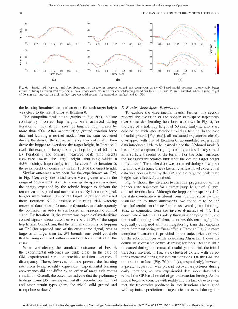
Fig. 6. Spatial rod (top), xr , and foot (bottom), x f , trajectories progress toward task completion as the GP-based model becomes incrementally betterinformed through accumulated experiential data. Trajectories measured for control-learning Iterations 0–3, 6, 10, and 15 are illustrated, where a jump heightof 60 mm was targeted on each surface type (a) solid ground, (b) trampoline surface, and (c) GM.

the learning iterations, the median error for each target heightwas close to the initial error at Iteration 0.

The trampoline peak height graphs in Fig. 5(b), indicateconsistently incorrect hop heights were achieved duringIteration 0; they all fell short of targeted hop heights bymore than 40%. After accumulating ground reaction forcedata and learning a revised model from the data recoveredduring Iteration 0, the subsequently synthesized control thendrove the hopper to overshoot the target height, in Iteration 1(with the exception being the target hop height of 60 mm).By Iteration 6 and onward, measured peak jump heightsconverged toward the target height, remaining within a±5% vicinity. Importantly, from Iteration 3 to Iteration 6,the peak height outcomes lay within 10% of the target height.

Similar outcomes were seen for the experiments on GM,in Fig. 5(c); only, the initial errors were greater and in therange of 55% − 65%. As GM is energy dissipative in nature,the energy expended by the robotic hopper to deform theterrain was dissipated and never restored. By Iteration 3, peakheights were within 10% of the target height and remainedthere. Iterations 6–10 consisted of learning trials wherebyrecovered data better informed the dynamics, and subsequentlythe optimizer, in order to synthesize an appropriate controlsignal. By Iteration 10, the system was capable of synthesizingcontrol signals whose outcomes were within 5% of the targethop height. Considering that the natural variability of hoppingon GM (for repeated runs of the exact same signal) was aslarge as or larger than the 5% bounds, one could concludethat learning occurred within seven hops for almost all of thecases.

When considering the simulated outcomes of Fig. 3,the experimental outcomes are quite close. In the case ofGM, experimental variation provides additional sources ofdiscrepancy. These, however, do not prevent the learningrate from being roughly equivalent; experimental learningconvergence did not differ by an order of magnitude versussimulation. Overall, the outcomes indicate that the preliminaryfindings from [35] are experimentally reproducible for GMand other terrain types (here, the trivial solid ground andtrampoline surfaces).

E. Results: State Space ExplorationTo explore the experimental results further, this section

reviews the evolution of the hopper state–space trajectoriesover successive learning iterations, as shown in Fig. 6, forthe case of a task hop height of 60 mm. Early iterations arecolored red with later iterations trending to blue. In the caseof solid ground [Fig. 6(a)], all measured trajectories closelyoverlapped with that of Iteration 0; accumulated experientialdata introduced little to be learned since the GP-based model’sbaseline presumption of rigid ground dynamics already servedas a sufficient model of the terrain. For the other surfaces,the measured trajectories undershot the desired target heightin Iteration 0. The undershoot was corrected during subsequentiterations, with trajectories clustering as less novel experientialdata was accumulated by the GP, and the targeted peak jumpheight was effectively attained.

Fig. 7 shows the iteration-to-iteration progression of thehopper state trajectory for a target jump height of 60 mm,on each terrain class. Although the hopper state space is 4-D,the state coordinate α is absent from this plot since we mayvisualize up to three dimensions. We found α to be theleast influential coordinate for the recovered ground forcing,Fsub, as computed from the inverse dynamics of (1). Thecoordinate α informs (1) solely through a damping term, cα;the small damping coefficient, c, makes this term negligible,especially compared with its neighboring term that capturesmore dominant spring stiffness effects. Through Fig. 7, a morecomplete illustration is provided of the trajectories exploredby the robotic hopper while exercising Algorithm 1 over thecourse of successive control-learning attempts. Because littleis learned during the course of a solid ground trial, the initialtrajectory traveled, in Fig. 7(a), clustered closely with trajec-tories measured during subsequent iterations. On the GM andtrampoline surfaces [Fig. 7(b) and (c), respectively], however,a greater separation was present between trajectories duringearly iterations, as new experiential data more drasticallyrefined the GP-based model of ground reaction forcing. As themodel began to coincide with reality and the task objective wasmet, the trajectories produced in later iterations also alignedwith optimizer predictions. Trajectories measured during late




Fig. 7. Stance phase hopper state trajectories explored over successive iterations for a target jump height of 60 mm (a) solid ground, (b) trampoline surface,and (c) GM.

Fig. 8. Predicted (dashed red) versus measured (dark green) ground forcing (a) solid ground, (b) trampoline surface, and (c) GM.

iterations incurred only minor changes, having already accom-plished the desired task.

F. Results: Ground Reaction Force Prediction

Success at the task objective relies on accurate force pre-diction for the synthesis of a task-achieving control signal.Using force recovery via inverse dynamics of (1), as employedfor learning, we compare actual ground reaction forcing,recovered from measured jump trajectories, with the forcepredictions used to craft the corresponding control.

The GP-based model of Fsub entails a baseline assumptionof rigid ground dynamics, in the absence of any training data.Then, we expect the predicted ground forces to coincide withthe recovered ground forcing in the solid ground experiments.

Because the true ground forcing model should already closelycoincide with the baseline assumption of (7), in this context,Iterations 1 and onward should introduce few if any, drasticdefects with respect to the baseline solid ground dynamics.Fig. 8(a) shows a comparison of the predicted and actualrecovered ground reaction forcing, applied by solid groundterrain, over the course of 15 control-learning iterations wherea target peak jump height of 60 mm was commanded. Groundreaction force predictions align very closely with actual recov-ered measurements of Fsub in most iterations. Shaded greenshows a 2 SD region associated with force measurements.Associated measurements of the area under the plots are foundabove and to the left of each plot.

The trampoline and GM cases are a bit more interesting.The underestimated trampoline forcing in Iteration 0 of




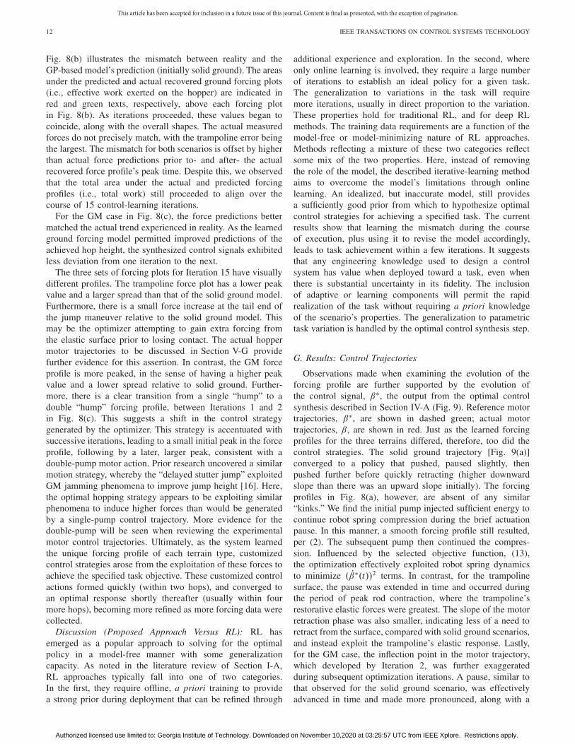
Fig. 8(b) illustrates the mismatch between reality and theGP-based model’s prediction (initially solid ground). The areasunder the predicted and actual recovered ground forcing plots(i.e., effective work exerted on the hopper) are indicated inred and green texts, respectively, above each forcing plotin Fig. 8(b). As iterations proceeded, these values began tocoincide, along with the overall shapes. The actual measuredforces do not precisely match, with the trampoline error beingthe largest. The mismatch for both scenarios is offset by higherthan actual force predictions prior to- and after- the actualrecovered force profile’s peak time. Despite this, we observedthat the total area under the actual and predicted forcingprofiles (i.e., total work) still proceeded to align over thecourse of 15 control-learning iterations.

For the GM case in Fig. 8(c), the force predictions bettermatched the actual trend experienced in reality. As the learnedground forcing model permitted improved predictions of theachieved hop height, the synthesized control signals exhibitedless deviation from one iteration to the next.

The three sets of forcing plots for Iteration 15 have visuallydifferent profiles. The trampoline force plot has a lower peakvalue and a larger spread than that of the solid ground model.Furthermore, there is a small force increase at the tail end ofthe jump maneuver relative to the solid ground model. Thismay be the optimizer attempting to gain extra forcing fromthe elastic surface prior to losing contact. The actual hoppermotor trajectories to be discussed in Section V-G providefurther evidence for this assertion. In contrast, the GM forceprofile is more peaked, in the sense of having a higher peakvalue and a lower spread relative to solid ground. Further-more, there is a clear transition from a single “hump” to adouble “hump” forcing profile, between Iterations 1 and 2in Fig. 8(c). This suggests a shift in the control strategygenerated by the optimizer. This strategy is accentuated withsuccessive iterations, leading to a small initial peak in the forceprofile, following by a later, larger peak, consistent with adouble-pump motor action. Prior research uncovered a similarmotion strategy, whereby the “delayed stutter jump” exploitedGM jamming phenomena to improve jump height [16]. Here,the optimal hopping strategy appears to be exploiting similarphenomena to induce higher forces than would be generatedby a single-pump control trajectory. More evidence for thedouble-pump will be seen when reviewing the experimentalmotor control trajectories. Ultimately, as the system learnedthe unique forcing profile of each terrain type, customizedcontrol strategies arose from the exploitation of these forces toachieve the specified task objective. These customized controlactions formed quickly (within two hops), and converged toan optimal response shortly thereafter (usually within fourmore hops), becoming more refined as more forcing data werecollected.

Discussion (Proposed Approach Versus RL): RL hasemerged as a popular approach to solving for the optimalpolicy in a model-free manner with some generalizationcapacity. As noted in the literature review of Section I-A,RL approaches typically fall into one of two categories.In the first, they require offline, a priori training to providea strong prior during deployment that can be refined through

additional experience and exploration. In the second, whereonly online learning is involved, they require a large numberof iterations to establish an ideal policy for a given task.The generalization to variations in the task will requiremore iterations, usually in direct proportion to the variation.These properties hold for traditional RL, and for deep RLmethods. The training data requirements are a function of themodel-free or model-minimizing nature of RL approaches.Methods reflecting a mixture of these two categories reflectsome mix of the two properties. Here, instead of removingthe role of the model, the described iterative-learning methodaims to overcome the model’s limitations through onlinelearning. An idealized, but inaccurate model, still providesa sufficiently good prior from which to hypothesize optimalcontrol strategies for achieving a specified task. The currentresults show that learning the mismatch during the courseof execution, plus using it to revise the model accordingly,leads to task achievement within a few iterations. It suggeststhat any engineering knowledge used to design a controlsystem has value when deployed toward a task, even whenthere is substantial uncertainty in its fidelity. The inclusionof adaptive or learning components will permit the rapidrealization of the task without requiring a priori knowledgeof the scenario’s properties. The generalization to parametrictask variation is handled by the optimal control synthesis step.

G. Results: Control Trajectories

Observations made when examining the evolution of theforcing profile are further supported by the evolution ofthe control signal, β∗, the output from the optimal controlsynthesis described in Section IV-A (Fig. 9). Reference motortrajectories, β∗, are shown in dashed green; actual motortrajectories, β, are shown in red. Just as the learned forcingprofiles for the three terrains differed, therefore, too did thecontrol strategies. The solid ground trajectory [Fig. 9(a)]converged to a policy that pushed, paused slightly, thenpushed further before quickly retracting (higher downwardslope than there was an upward slope initially). The forcingprofiles in Fig. 8(a), however, are absent of any similar“kinks.” We find the initial pump injected sufficient energy tocontinue robot spring compression during the brief actuationpause. In this manner, a smooth forcing profile still resulted,per (2). The subsequent pump then continued the compres-sion. Influenced by the selected objective function, (13),the optimization effectively exploited robot spring dynamicsto minimize (β∗(t))2 terms. In contrast, for the trampolinesurface, the pause was extended in time and occurred duringthe period of peak rod contraction, where the trampoline’srestorative elastic forces were greatest. The slope of the motorretraction phase was also smaller, indicating less of a need toretract from the surface, compared with solid ground scenarios,and instead exploit the trampoline’s elastic response. Lastly,for the GM case, the inflection point in the motor trajectory,which developed by Iteration 2, was further exaggeratedduring subsequent optimization iterations. A pause, similar tothat observed for the solid ground scenario, was effectivelyadvanced in time and made more pronounced, along with a




Fig. 9. Synthesized control inputs (a) solid ground, (b) trampoline surface, and (c) GM.

Fig. 10. (a) Mean, over all experimental runs, of each of the reference and reduced training set cardinalities (|| and ||, respectively) are compared across15 control-learning iterations. (b) Mean of ||, as a percentage of ||, is additionally depicted across successive iterations, demonstrating a linearly decreasingtrend; while || grows linearly, || grows sublinearly.

more gradual transition from the first short peak to the nextlarger peak. This feature signified the switch from a singlepush to a double push strategy as the optimization’s meansof exploiting the learned terrain dynamics. The convergedoptimal control solutions inherently depend on the GP-basedmodel of the terrain reaction forces. This computed controlinput evolves as the GP’s understanding of the terrain isincrementally refined.

H. Results: Training Set ReductionThe applied data curation procedure (Section III-D)

is designed to target system bottlenecks with respect tocomputational complexity and further facilitate onlineapplication. Computational costs are primarily driven by thecardinality of the training set used to train the GP-basedmodel, (7). Fig. 10(d) shows the accumulated cardinalities forthe full reference data set, , and the reduced set, , over the




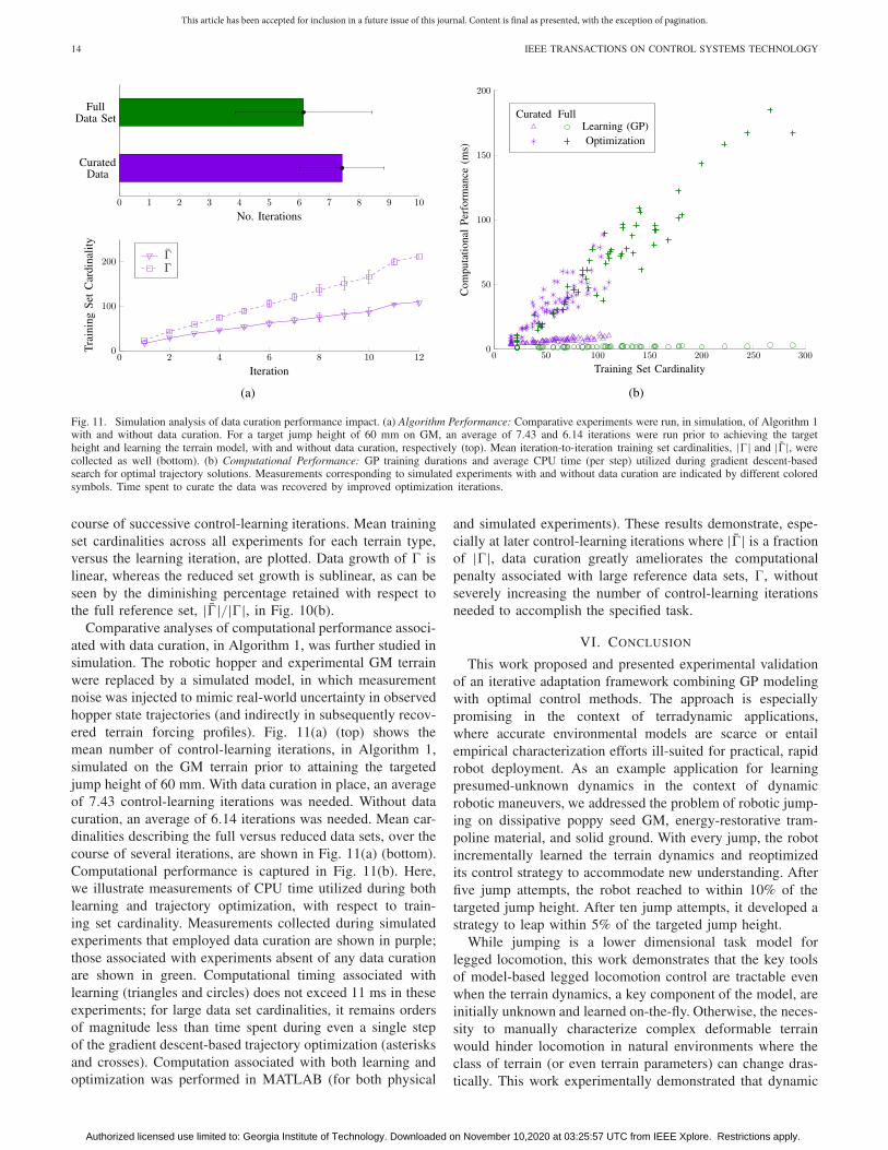
Fig. 11. Simulation analysis of data curation performance impact. (a) Algorithm Performance: Comparative experiments were run, in simulation, of Algorithm 1with and without data curation. For a target jump height of 60 mm on GM, an average of 7.43 and 6.14 iterations were run prior to achieving the targetheight and learning the terrain model, with and without data curation, respectively (top). Mean iteration-to-iteration training set cardinalities, || and ||, werecollected as well (bottom). (b) Computational Performance: GP training durations and average CPU time (per step) utilized during gradient descent-basedsearch for optimal trajectory solutions. Measurements corresponding to simulated experiments with and without data curation are indicated by different coloredsymbols. Time spent to curate the data was recovered by improved optimization iterations.

course of successive control-learning iterations. Mean trainingset cardinalities across all experiments for each terrain type,versus the learning iteration, are plotted. Data growth of islinear, whereas the reduced set growth is sublinear, as can beseen by the diminishing percentage retained with respect tothe full reference set, ||/||, in Fig. 10(b).

Comparative analyses of computational performance associ-ated with data curation, in Algorithm 1, was further studied insimulation. The robotic hopper and experimental GM terrainwere replaced by a simulated model, in which measurementnoise was injected to mimic real-world uncertainty in observedhopper state trajectories (and indirectly in subsequently recov-ered terrain forcing profiles). Fig. 11(a) (top) shows themean number of control-learning iterations, in Algorithm 1,simulated on the GM terrain prior to attaining the targetedjump height of 60 mm. With data curation in place, an averageof 7.43 control-learning iterations was needed. Without datacuration, an average of 6.14 iterations was needed. Mean car-dinalities describing the full versus reduced data sets, over thecourse of several iterations, are shown in Fig. 11(a) (bottom).Computational performance is captured in Fig. 11(b). Here,we illustrate measurements of CPU time utilized during bothlearning and trajectory optimization, with respect to train-ing set cardinality. Measurements collected during simulatedexperiments that employed data curation are shown in purple;those associated with experiments absent of any data curationare shown in green. Computational timing associated withlearning (triangles and circles) does not exceed 11 ms in theseexperiments; for large data set cardinalities, it remains ordersof magnitude less than time spent during even a single stepof the gradient descent-based trajectory optimization (asterisksand crosses). Computation associated with both learning andoptimization was performed in MATLAB (for both physical

and simulated experiments). These results demonstrate, espe-cially at later control-learning iterations where || is a fractionof ||, data curation greatly ameliorates the computationalpenalty associated with large reference data sets, , withoutseverely increasing the number of control-learning iterationsneeded to accomplish the specified task.

VI. CONCLUSION

This work proposed and presented experimental validationof an iterative adaptation framework combining GP modelingwith optimal control methods. The approach is especiallypromising in the context of terradynamic applications,where accurate environmental models are scarce or entailempirical characterization efforts ill-suited for practical, rapidrobot deployment. As an example application for learningpresumed-unknown dynamics in the context of dynamicrobotic maneuvers, we addressed the problem of robotic jump-ing on dissipative poppy seed GM, energy-restorative tram-poline material, and solid ground. With every jump, the robotincrementally learned the terrain dynamics and reoptimizedits control strategy to accommodate new understanding. Afterfive jump attempts, the robot reached to within 10% of thetargeted jump height. After ten jump attempts, it developed astrategy to leap within 5% of the targeted jump height.

While jumping is a lower dimensional task model forlegged locomotion, this work demonstrates that the key toolsof model-based legged locomotion control are tractable evenwhen the terrain dynamics, a key component of the model, areinitially unknown and learned on-the-fly. Otherwise, the neces-sity to manually characterize complex deformable terrainwould hinder locomotion in natural environments where theclass of terrain (or even terrain parameters) can change dras-tically. This work experimentally demonstrated that dynamic




locomotion tasks can be achieved precisely even when keysystem quantities begin poorly modeled or entirely unknown.Specifically, incremental learning of the unknown externalforcing, during the course of iterative control synthesis andexecution, can be accomplished in only a handful of repeti-tions. Though promising, one aspect not considered was safetyor stability during the learning iterations. We aim to considerthis in future efforts.

REFERENCES

[1] E. R. Westervelt, J. W. Grizzle, and D. E. Koditschek, “Hybrid zerodynamics of planar biped walkers,” IEEE Trans. Autom. Control, vol. 48,no. 1, pp. 42–56, Jan. 2003.

[2] I. R. Manchester, U. Mettin, F. Iida, and R. Tedrake, “Stable dynamicwalking over uneven terrain,” Int. J. Robot. Res., vol. 30, no. 3,pp. 265–279, Mar. 2011.

[3] A. D. Ames, “Human-inspired control of bipedal walking robots,” IEEETrans. Autom. Control, vol. 59, no. 5, pp. 1115–1130, May 2014.

[4] C. M. Hubicki, J. J. Aguilar, D. I. Goldman, and A. D. Ames, “Tractableterrain-aware motion planning on granular media: An impulsive jump-ing study,” in Proc. IEEE/RSJ Int. Conf. Intell. Robots Syst. (IROS),Oct. 2016, pp. 3887–3892.

[5] H. E. Taha, C. A. Woolsey, and M. R. Hajj, “Geometric control approachto longitudinal stability of flapping flight,” J. Guid., Control, Dyn.,vol. 39, no. 2, pp. 214–226, Feb. 2016.

[6] A. Ramezani, X. Shi, S.-J. Chung, and S. Hutchinson, “Lagrangianmodeling and flight control of articulated-winged bat robot,” inProc. IEEE/RSJ Int. Conf. Intell. Robots Syst. (IROS), Sep. 2015,pp. 2867–2874.

[7] S. D. Kelly, P. Pujari, and H. Xiong, “Geometric mechanics, dynamics,and control of fishlike swimming in a planar ideal fluid,” in NaturalLocomotion in Fluids and on Surfaces: Swimming, Flying, and Sliding,S. Childress, A. Hosoi, W. W. Schultz, and J. Wang, Eds. New York,NY, USA: Springer, 2012, pp. 101–116.

[8] K. A. Morgansen, B. I. Triplett, and D. J. Klein, “Geometric methodsfor modeling and control of free-swimming fin-actuated underwatervehicles,” IEEE Trans. Robot., vol. 23, no. 6, pp. 1184–1199, Dec. 2007.

[9] M. Porez, F. Boyer, and A. J. Ijspeert, “Improved lighthill fish swim-ming model for bio-inspired robots: Modeling, computational aspectsand experimental comparisons,” Int. J. Robot. Res., vol. 33, no. 10,pp. 1322–1341, Sep. 2014.

[10] J. Wang and X. Tan, “Averaging tail-actuated robotic fish dynamicsthrough force and moment scaling,” IEEE Trans. Robot., vol. 31, no. 4,pp. 906–917, Aug. 2015.

[11] V. Vasilopoulos, I. S. Paraskevas, and E. G. Papadopoulos, “Compliantterrain legged locomotion using a viscoplastic approach,” in Proc.IEEE/RSJ Int. Conf. Intell. Robots Syst., Sep. 2014, pp. 4849–4854.

[12] F. B. Mathis and R. Mukherjee, “Two-mass robot hopping on an elasticfoundation: Apex height control,” in Proc. IEEE 1st Int. Conf. Control,Meas. Instrum. (CMI), Jan. 2016, pp. 167–171.

[13] D. Koepl and J. Hurst, “Impulse control for planar spring-mass running,”J. Intell. Robotic Syst., vol. 74, nos. 3–4, pp. 589–603, Jun. 2014.

[14] H.-J. Kang et al., “Biped walking stabilization on soft ground based ongait analysis,” in Proc. 4th IEEE RAS EMBS Int. Conf. Biomed. Robot.Biomechatronics (BioRob), Jun. 2012, pp. 669–674.

[15] W. Bosworth, J. Whitney, S. Kim, and N. Hogan, “Robot locomotionon hard and soft ground: Measuring stability and ground propertiesin-situ,” in Proc. IEEE Int. Conf. Robot. Autom. (ICRA), May 2016,pp. 3582–3589.

[16] J. Aguilar and D. I. Goldman, “Robophysical study of jumping dynamicson granular media,” Nature Phys., vol. 12, pp. 278–283, Nov. 2016.

[17] C. Li, T. Zhang, and D. I. Goldman, “A terradynamics of legged loco-motion on granular media,” Science, vol. 339, no. 6126, pp. 1408–1412,Mar. 2013.

[18] A. Gijsberts and G. Metta, “Real-time model learning using incrementalsparse spectrum Gaussian process regression,” Neural Netw., vol. 41,pp. 59–69, May 2013.

[19] D. Nguyen-Tuong, B. Scholkopf, and J. Peters, “Sparse online modellearning for robot control with support vector regression,” in Proc.IEEE/RSJ Int. Conf. Intell. Robots Syst., Oct. 2009, pp. 3121–3126.

[20] S. Vijayakumar, A. D’Souza, and S. Schaal, “Incremental online learningin high dimensions,” Neural Comput., vol. 17, no. 12, pp. 2602–2634,Dec. 2005.

[21] M. P. Deisenroth, D. Fox, and C. E. Rasmussen, “Gaussian processesfor data-efficient learning in robotics and control,” IEEE Trans. PatternAnal. Mach. Intell., vol. 37, no. 2, pp. 408–423, Feb. 2015.

[22] S. Levine and P. Abbeel, “Learning neural network policies with guidedpolicy search under unknown dynamics,” in Proc. Adv. Neural Inf.Process. Syst., 2014, pp. 1071–1079.

[23] J. Boedecker, J. T. Springenberg, J. Wulfing, and M. Riedmiller,“Approximate real-time optimal control based on sparse Gaussianprocess models,” in Proc. IEEE Symp. Adapt. Dyn. Program. Reinforce-ment Learn. (ADPRL), Dec. 2014, pp. 1–8.

[24] Y. Pan and E. A. Theodorou, “Data-driven differential dynamic program-ming using Gaussian processes,” in Proc. Amer. Control Conf. (ACC),Jul. 2015, pp. 4467–4472.

[25] Y. Pan, X. Yan, E. Theodorou, and B. Boots, “Scalable reinforcementlearning via trajectory optimization and approximate Gaussian processregression,” in Proc. NIPS Workshop Adv. Approx. Bayesian Inference,2015, pp. 1–5.

[26] Y. Pan, X. Yan, E. Theodorou, and B. Boots, “Adaptive probabilis-tic trajectory optimization via efficient approximate inference,” 2016,arXiv:1608.06235. [Online]. Available: http://arxiv.org/abs/1608.06235

[27] H. Modares, F. L. Lewis, and M.-B. Naghibi-Sistani, “Integral rein-forcement learning and experience replay for adaptive optimal controlof partially-unknown constrained-input continuous-time systems,” Auto-matica, vol. 50, no. 1, pp. 193–202, Jan. 2014.

[28] G. Chowdhary, “Concurrent learning for convergence in adaptive controlwithout persistency of excitation,” Ph.D. dissertation, School Aerosp.Eng., Georgia Inst. Technol., Atlanta, GA, USA, 2010.

[29] G. Chowdhary, T. Yucelen, M. Mühlegg, and E. N. Johnson, “Concurrentlearning adaptive control of linear systems with exponentially conver-gent bounds,” Int. J. Adapt. Control Signal Process., vol. 27, no. 4,pp. 280–301, Apr. 2013.

[30] H. A. Kingravi, G. Chowdhary, P. A. Vela, and E. N. Johnson, “Repro-ducing kernel Hilbert space approach for the online update of radialbases in neuro-adaptive control,” IEEE Trans. Neural Netw. Learn. Syst.,vol. 23, no. 7, pp. 1130–1141, Jul. 2012.

[31] G. Chowdhary, H. A. Kingravi, J. P. How, and P. A. Vela, “Bayesiannonparametric adaptive control using Gaussian processes,” IEEE Trans.Neural Netw. Learn. Syst., vol. 26, no. 3, pp. 537–550, Mar. 2015.

[32] H. Kingravi, “Reduced-set models for improving the training andexecution speed of kernel methods,” Ph.D. dissertation, School Elect.Comput. Eng., Georgia Inst. Technol., Atlanta, GA, USA, 2014.

[33] J. Hidalgo-Carrio, D. Hennes, J. Schwendner, and F. Kirchner, “Gaussianprocess estimation of odometry errors for localization and mapping,” inProc. IEEE Int. Conf. Robot. Autom. (ICRA), May 2017, pp. 5696–5701.

[34] C. Cunningham, M. Ono, I. Nesnas, J. Yen, and W. L. Whittaker,“Locally-adaptive slip prediction for planetary rovers using Gaussianprocesses,” in Proc. IEEE Int. Conf. Robot. Autom. (ICRA), May 2017,pp. 5487–5494.

[35] A. H. Chang, C. M. Hubicki, J. J. Aguilar, D. I. Goldman, A. D. Ames,and P. A. Vela, “Learning to jump in granular media: Unifying optimalcontrol synthesis with Gaussian process-based regression,” in Proc. IEEEInt. Conf. Robot. Autom. (ICRA), May 2017, pp. 2154–2160.

[36] A. Hereid, E. A. Cousineau, C. M. Hubicki, and A. D. Ames, “3Ddynamic walking with underactuated humanoid robots: A direct collo-cation framework for optimizing hybrid zero dynamics,” in Proc. IEEEInt. Conf. Robot. Autom. (ICRA), May 2016, pp. 1–8.

[37] X. Xiong, A. D. Ames, and D. I. Goldman, “A stability region criterionfor flat-footed bipedal walking on deformable granular terrain,” inProc. IEEE/RSJ Int. Conf. Intell. Robots Syst. (IROS), Sep. 2017,pp. 4552–4559.

[38] F. Berkenkamp, R. Moriconi, A. P. Schoellig, and A. Krause, “Safelearning of regions of attraction for uncertain, nonlinear systems withGaussian processes,” in Proc. IEEE 55th Conf. Decis. Control (CDC),Dec. 2016, pp. 4661–4666.

[39] F. Berkenkamp, A. P. Schoellig, and A. Krause, “Safe controller opti-mization for quadrotors with Gaussian processes,” in Proc. IEEE Int.Conf. Robot. Autom. (ICRA), May 2016, pp. 493–496.

[40] C. D. McKinnon and A. P. Schoellig, “Learning multimodal models forrobot dynamics online with a mixture of Gaussian process experts,” inProc. IEEE Int. Conf. Robot. Autom. (ICRA), May 2017, pp. 322–328.

[41] A. H. Chang, C. Hubicki, A. Ames, and P. A. Vela, “Every hopis an opportunity: Quickly classifying and adapting to terrain duringtargeted hopping,” in Proc. Int. Conf. Robot. Autom. (ICRA), May 2019,pp. 3188–3194.

[42] C. Hubicki and J. Hurst, “Running on soft ground: Simple, energy-optimal disturbance rejection,” in Proc. CLAWAR, 2012, pp. 543–547.




[43] K. P. Murphy, Machine Learning: A Probabilistic Perspective.Cambridge, MA, USA: Massachusetts Institute of Technology, 2012.

[44] S. Ba and V. R. Joseph, “Composite Gaussian process models foremulating expensive functions,” Ann. Appl. Statist., vol. 6, no. 4,pp. 1838–1860, Dec. 2012.

[45] H. A. Kingravi, P. A. Vela, and A. Gray, “Reduced set KPCA forimproving the training and execution speed of kernel machines,” in Proc.SIAM Int. Conf. Data Mining, May 2013, pp. 441–449.

[46] C. R. Hargraves and S. W. Paris, “Direct trajectory optimizationusing nonlinear programming and collocation,” J. Guid., Control, Dyn.,vol. 10, no. 4, pp. 338–342, Jul. 1987.

[47] A. V. Rao, “A survey of numerical methods for optimal control,” Adv.Astron. Sci., vol. 135, no. 1, pp. 497–528, Aug. 2009.

[48] M. S. Jones, “Optimal control of an underactuated bipedal robot,” Ph.D.dissertation, School Mech., Ind., Manuf. Eng., Oregon State Univ.,Corvallis, OR, USA, 2014.

[49] A. Wächter and L. T. Biegler, “On the implementation of an interior-point filter line-search algorithm for large-scale nonlinear programming,”Math. Program., vol. 106, no. 1, pp. 25–57, 2006.

Alexander H. Chang (Member, IEEE) received thebachelor’s degree in computer and telecommunica-tions engineering and the master’s degree in electri-cal engineering from the University of Pennsylvania,Philadelphia, PA, USA, in 2005 and 2006, respec-tively. He is currently pursuing the robotics Ph.D.degree with the Intelligent Vision and Automa-tion Laboratory, School of Electrical and ComputerEngineering, Institute for Robotics and IntelligentMachines, Georgia Institute of Technology, Atlanta,GA, USA, under the supervision of ProfessorPatricio A. Vela.

His research interests focus on biologically inspired robotic locomotion,specifically snakelike robotic motion modeling and control.

Christian M. Hubicki (Member, IEEE) receivedthe bachelor’s and master’s degrees in mechanicalengineering, with minor degrees in physics andmusic, from Bucknell University, Lewisburg, PA,USA, in 2007 and 2011, respectively, and the dualPh.D. degree in robotics and mechanical engineeringfrom Oregon State University, Corvallis, OR, USA,in 2015.

In 2015, he joined the Georgia Institute ofTechnology, Atlanta, GA, USA, where he wasa Post-Doctoral Fellow with the Department of

Mechanical Engineering and the School of Physics. In 2018, he started hisposition as the Director of the Optimal Robotics Laboratory, Florida StateUniversity, Tallahassee, FL, USA, with research specializing in legged roboticsand applied optimization. He is currently an Assistant Professor of mechanicalengineering with Florida State University and the FAMU-FSU College ofEngineering, Tallahassee, FL, USA.

Dr. Hubicki was a recipient of the Gilbreth Lectureship from the NationalAcademy of Engineering in 2020.

Jeffrey J. Aguilar received the B.S., master’s, andPh.D. degrees in mechanical engineering from theGeorgia Institute of Technology, Atlanta, GA, USA,in 2010, 2012, and 2016, respectively.

During his graduate program, he worked in theCRAB Laboratory, Georgia Institute of Technology,and utilized a simple robotic system to study thedynamics of jumping on hard substrates and gran-ular media. He is currently Managing Engineer-ing of research and development with Hi FidelityGenetics, Durham, NC, USA, a startup focused on

developing new sensor technologies to collect data for computational cropbreeding. His work has involved the creation of the RootTracker, a scalablecapacitance-based sensor for mapping in-field root systems.

Daniel I. Goldman received the B.S. degree inphysics from the Massachusetts Institute of Tech-nology, Cambridge, MA, USA, in 1994, and thePh.D. degree with a focus on nonlinear dynamicsand granular media from The University of Texas atAustin, Austin, TX, USA, in 2002.

He was a Post-Doctoral Researcher in locomotionbiomechanics with the University of California atBerkeley, Berkeley, CA, USA. He became a FacultyMember with the Georgia Institute of Technology,Atlanta, GA, USA, in 2007, where he also became

an Adjunct Member with the School of Biology and a member of theBioengineering Graduate Program. He is currently a Dunn Family Professorwith the School of Physics, Georgia Institute of Technology. His researchprogram investigates the interaction of biological and physical systems withcomplex materials, including granular media.

Prof. Goldman is a Georgia Power Professor of Excellence and a Fellow ofthe American Physical Society. He received the NSF CAREER/PECASEAward, the DARPA Young Faculty Award, the Sigma Xi Young FacultyAward, and the Burroughs Welcome Fund Career Award at the ScientificInterface.

Aaron D. Ames (Senior Member, IEEE) receivedthe B.S. degree in mechanical engineering and theB.A. degree in mathematics from the University ofSt. Thomas, St. Paul, MN, USA, in 2001, and theM.A. degree in mathematics and the Ph.D. degree inelectrical engineering and computer sciences fromthe University of California at Berkeley, Berkeley,CA, USA, in 2006.

He was a Post-Doctoral Scholar at the CaliforniaInstitute of Technology, Pasadena, CA, USA, from2006 to 2008. He began his faculty career at Texas

A&M University, College Station, TX, USA, in 2008. He was subsequentlyan Associate Professor in mechanical engineering and electrical and computerengineering with the Georgia Institute of Technology, Atlanta, GA, USA.He is currently the Bren Professor of mechanical and civil engineering andcontrol and dynamical systems at the California Institute of Technology. Hislaboratory designs build and test novel bipedal robots, exoskeletons, andprostheses with the goal of achieving human-like robotic locomotion. Hisresearch interests span the areas of robotics, safety-critical nonlinear control,and hybrid systems.

Dr. Ames received the NSF CAREER, Eckman, and Ruberti awards, amongothers.

Patricio A. Vela (Member, IEEE) received theB.Sc. and Ph.D. degrees in control and dynamicalsystems from the California Institute of Technology,Pasadena, CA, USA, in 1998 and 2003, respectively,where his graduate research focused on geometricnonlinear control and robotics.

In 2004, he was a Post-Doctoral Researcher incomputer vision with the School of Electrical andComputer Engineering (ECE), Georgia Institute ofTechnology, Atlanta, GA, USA, He joined the ECEFaculty, Georgia Institute of Technology, in 2005,

where he is currently an Associate Professor with the School of ECE,Institute of Robotics and Intelligent Machines. His research interests liein the geometric perspectives to control theory, computer vision, the rolethat computer vision can play for achieving control-theoretic objectives of(semi-)autonomous systems, and the control of nonlinear systems, typicallyrobotic systems.


Learning Terrain Dynamics: A Gaussian Process Modeling …

Documents

Transcript of Learning Terrain Dynamics: A Gaussian Process Modeling …