Six SigmaGreen Belt Training

6Methusael Brown Cebrian ITIL v3 LSSBB

Certified Lean Six Sigma Black Belt

“You cannot Manage, what you cannot measure” – W. Edwards Deming

What is Six Sigma?

- It is a Quantitative, data-driven Define, Measure, Analyze, Improve, Control methodology to Process Improvement based on Statistical and Management tools to increase efficiency in the process.

- Simply put, it is a way of using data to solve problems and make businesses more profitable. 

The term “sigma” is used to designate the distribution or spread around the mean (average) of any process or procedure.

• Developed by Motorola, used successfully by Texas Instruments, Boeing, Honeywell, Lockheed Martin.

• GE, has become the face of Six Sigma due to its wide adoption throughout the organization.

• Internal Focus: Improve existing processes – manufacturing, business transaction for service industry.

• External Focus: Listens to Voice of the Customer (VoC).

• Uses trained teams- Champions: Business Leaders, provide resources

and support implementation.- Master Black Belts: Experts and Culture-

Changers, train and mentor Black Belts/ Green Belts.- Black Belts: Lead Six Sigma project teams.- Green Belts: Carry out six sigma projects related

to their jobs.Driver for Cost Savings and Customer Satisfaction

Six Sigma is:• An enabler to Business Strategy.• Places customers at the center of the performance

improvements.• Fact-based approach for improving business

processes and solving problems.• A proven methodology and toolset supported by

deep training and mentoring.• Focused on reducing variability of processes• Elimination of Defects/Wastes (Mudas).• A way to develop highly skilled business leaders.• A means for creating capacity in organizations.

Quality is Everyone’s Responsibility

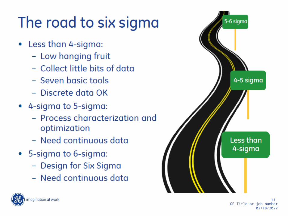
Striving towards Six Sigma

Six Sigma Improves Quality by Reducing Defects and Variation

Quality

99% is never good enough!

Building on Quality reduces long -term costs

Why do we need to pursue Quality Initiatives?• Meet Customer expectations for higher quality.• Provide a competitive differentiator in the Market.• Build greater pride and satisfaction within the company.• Drive other key goals: Productivity and Growth.

Delighting Customers

• Making customers successful• Customer-Centric metrics• Listens to the Voice of the Customer

(Voc)• Surveys, Interviews, Net Promoter Score

Make customers feel Six Sigma

The Kano Model• A way to evaluate how customer satisfaction is

impacted by an initiative

• Three types of improvements• Hygiene factor (green). Customer expect this and

is dissatisfied if not fulfilled. Ensuring that these

needs are met should have highest priority.

• Performance factor (blue). There is a relationship

between customer satisfaction and how well the

need is met. Important to ensure satisfactory

performance.

• Delight factor (red). Customers do not expect this

and are thus indifferent if the need is not met. A

way to create additional satisfaction if all hygiene

factors are performing.

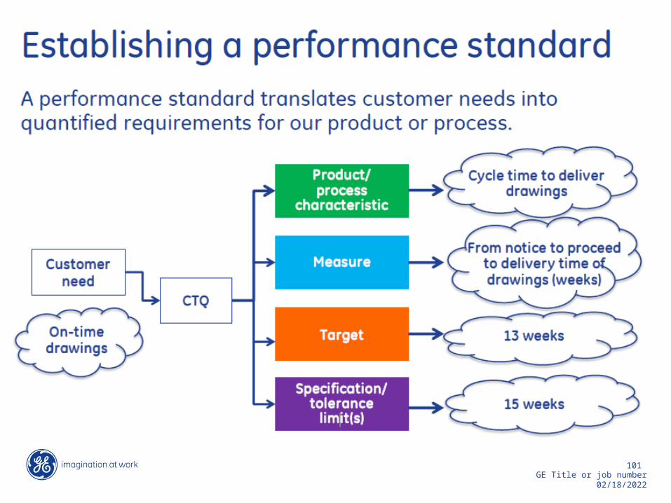
Definitions

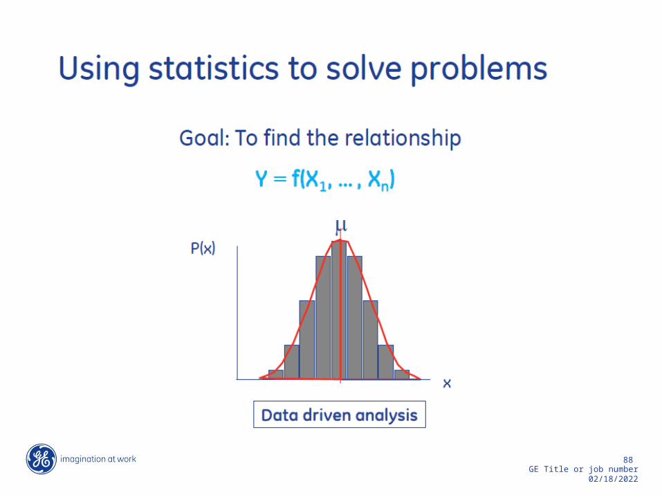
The statistical objective of Six Sigma

Reduce Variation and Center Process – Customers feel variation more than the mean.

What is Variation?• Variation is the extent to which items (things) differ,

from one to the next!• There will always be some variation present in all

processes.-Nature – shape, size of leaves, height of trees-Human – Handwriting, speed of walk, tone of

voice etc.-Mechanical – weight/size/shape of product,

content etc.

We can tolerate this variation if:- The process is on target (where we want it to be)- The variation is small compared to the customer

specifications.- The process is stable over time.

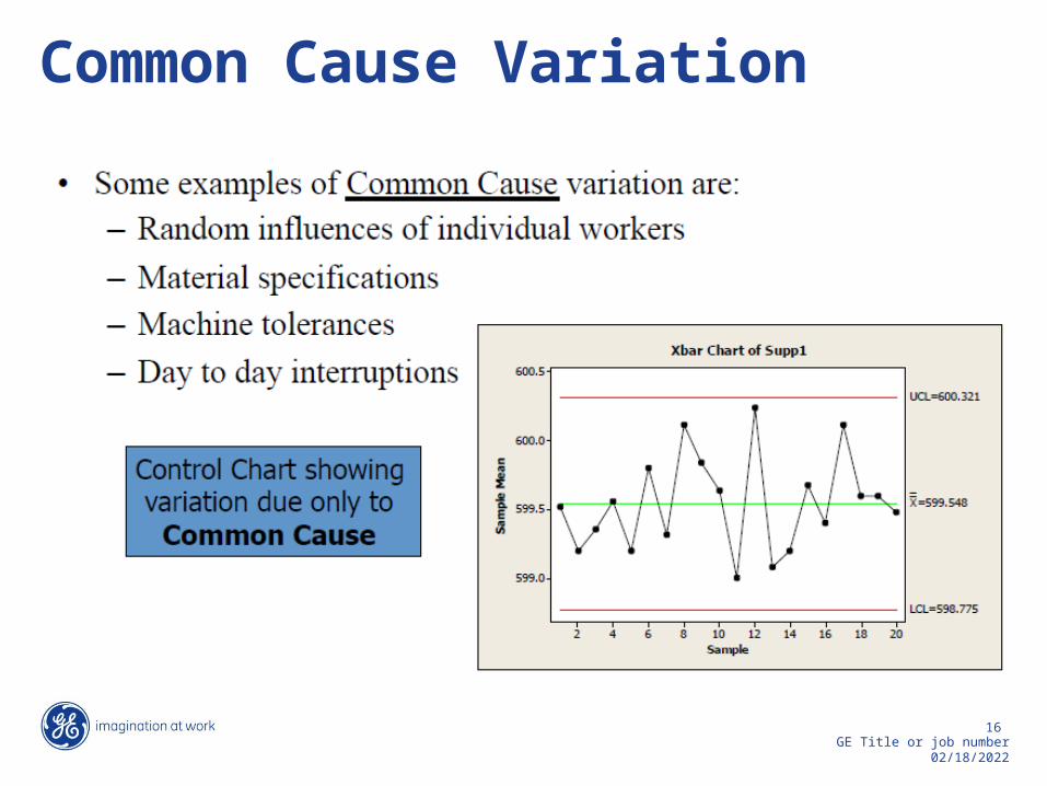
According to Deming:• 85%-95% of all variation is Common

Cause.• 5%-15% of all variation is Special

Cause.• Common Cause – variation is

random, stable and consistent over time. It is expected variation.

• Special Cause – is not random, and changes over time. It is unexpected variation. There is undue influence in the process.

Variation is the enemy of Process Improvement efforts.

Common Cause Variation

Special Cause Variation

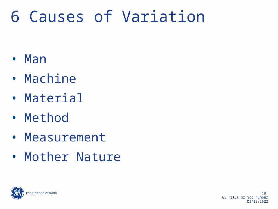
6 Causes of Variation

• Man• Machine• Material• Method• Measurement• Mother Nature

ProcessAny activity that takes inputs, adds value, and provides an output(s).

Variation exists in the process.

Six Sigma improvement approach

Six Sigma is Long Term Commitment to the Philosophy of Quality.

The heart of Six Sigma

Historically the Y – with Six Sigma the X’s

Focusing on the X’s relies on a good and steady flow of Data – Metrics!

D-M-A-I-C

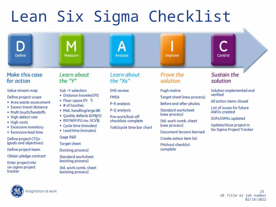
Lean Six Sigma Checklist

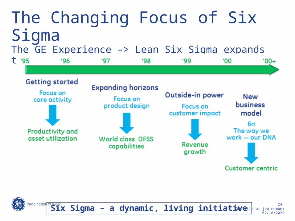
The Changing Focus of Six SigmaThe GE Experience –> Lean Six Sigma expands the tool set

Six Sigma – a dynamic, living initiative

Summary of Introduction:

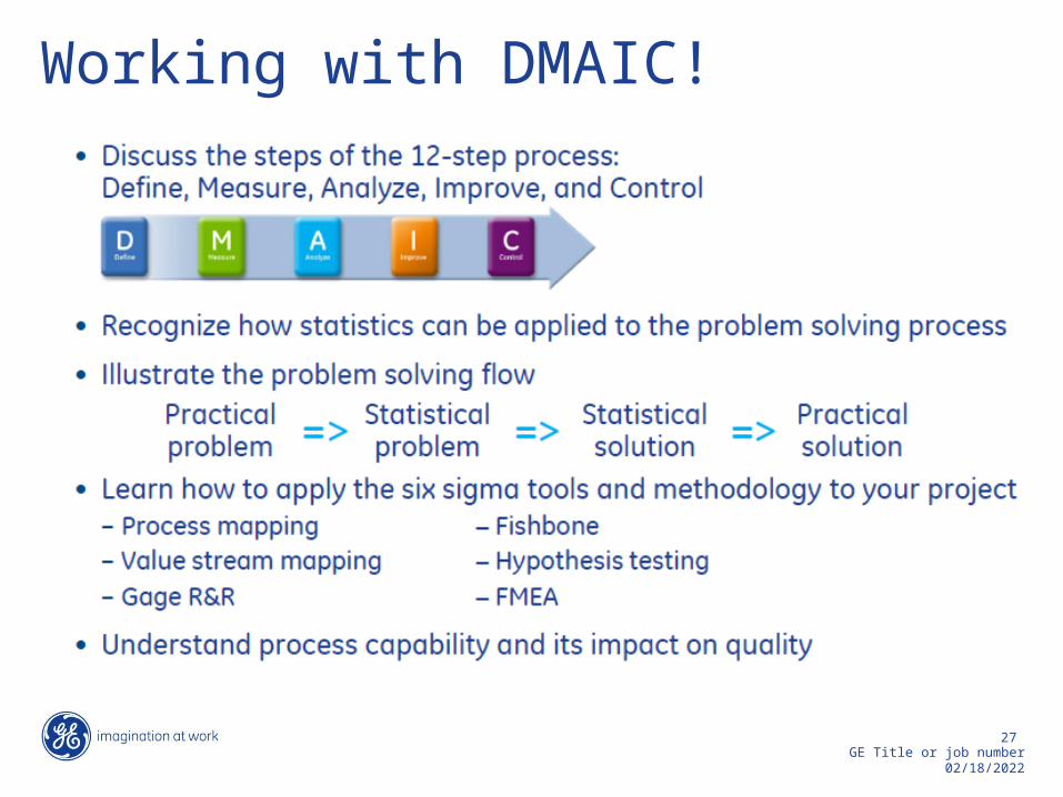
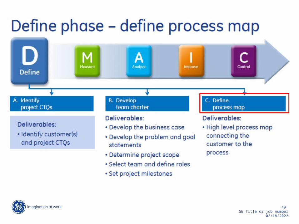
Working with DMAIC!

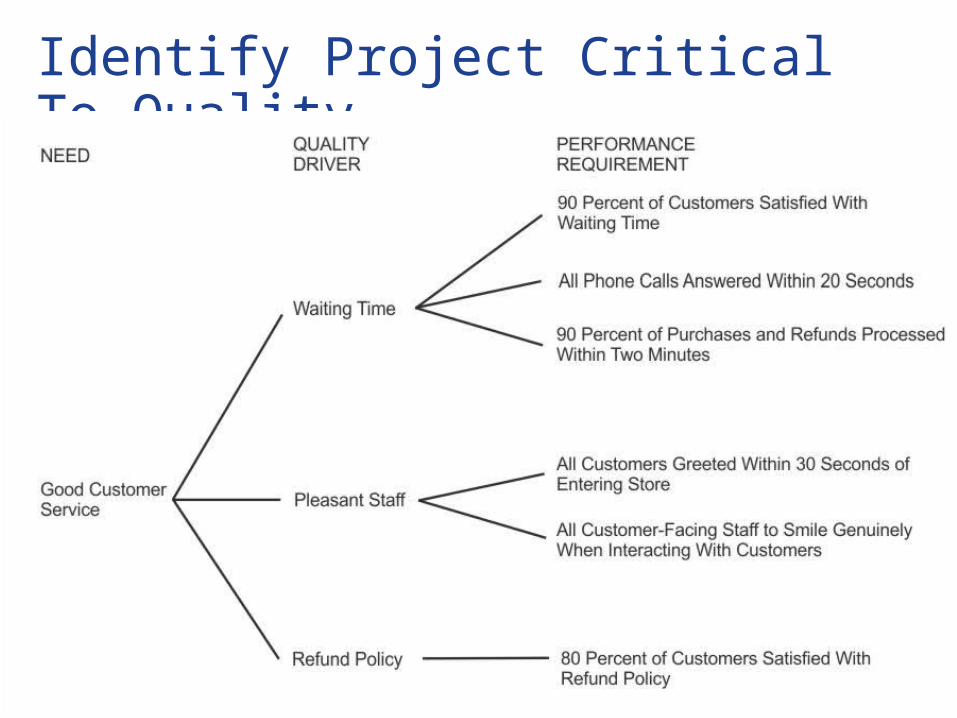
Identify Project Critical To Quality

Define Phase Date Version 1.1

The scope of this project will focus on following key aspects:

People

Process

Critical To Quality

Machines

Workplace

Problem / Goal RolesSponsorBBGB

Shift Managers:Allan K, Mark L., John Doe

Shift Machine OperatorsRey M , Louie G, Rick L.

Finance AccountantJulie P.

Project Outcome MilestonesDefine 1-Jun-13

Measure 15-Jun-13

Analyze 15-Jul-13

Improve 15-Oct-13

Control 15-Nov-13

Potential RisksLack of Buy in from operatorsNon-Compliance to governance/policy/SOP and difficult to monitorLack of support from Leadership Signature Sponsor Signature BB / GB

We will look at the existing capabilities of the machines to produce the PCB's according to specifications. Including the ways it processes the raw materials being fed to it, as well as its technological limitations to produce a PCB according to specs.We will look at the workplace environment involved in the process of producing PCB's. IF an essential 5S processes are in place. Some aspects that will be looked at, but is not limited to: Machine arrangements, distance, tool placements, lighting, tidiness.

The existing process produces a high number of scraps or waste, which affects the pricing model for the product as well as the reliability of delivery schedules, we will pursue key areas of interests such as People, Process, Machines, and Workplace in zeroing down the root causes of the existing issues. In order to meet the Customer requirements for Volumes, we will embark on a project using Lean Six Sigma methodologies to improve the existing process by eliminating 98% from existing Scrap Rates, reduce product cost as well as achieve 100% reliability in delivery schedule. With the elimination of Scraps in the processes, we will be able to provide room for future growth in customer demands.

98% Reduction of Scraps 100% Availablity of Machines to Operate Newly trained Operators Newly published SOP's, Policy, Guideline and Manuals Reduced Product Cost 100% Reliability in Delivery Schedule 35% increase in volume capacity

Plant Manager - David MackQuality Manager - John Loyd

Methusael B. Cebrian

Core Team

Project Charter

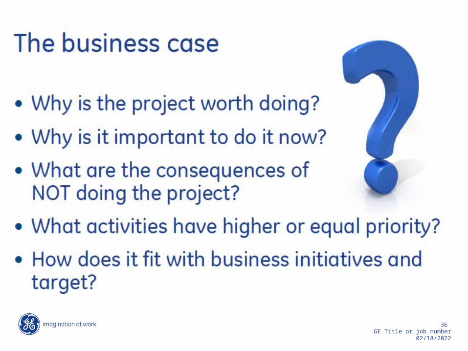
The Quality and Reliability of our process and products are threatened because of the defects existing in the manufacturing line. Customers are complaining that we can no longer keep up with our committed scheduled deliveries, which also affects their supply chain. The cost of raw materials is also at all time high, and a high rate of scraps is no longer acceptable. The high cost of raw materials and the number of scrap rates, is passed to the customer which coupled with unreliable delivery schedule makes our customers to look for other suppliers. It is therefore imperative to engage the problem and eliminate it using Lean Six Sigma methodology and make our product a reliable and cost competetive one for our customers.

Project NameBusiness Case Project Scope

Eliminate Manufacturing Defects Affecting Scrap Rate, Product Cost and Delivery Schedule.

1-Jul-13

We will look at the skill sets, trainings, and capabilities of people involved in the process, to follow the existing instructions, guidelines and SOP's needed to produce the PCB's.

We will look at the existing methodologies, instructions, steps if it conforms to the right processes needed to produce the PCB's according to specifications.

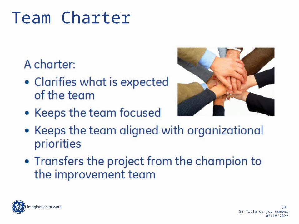
Team Charter

Five major elements of a Charter

Problem and Goal Statements

Together they provide focus and purpose for the team

Description of the “pain”

Problem Statement

The Goal Statement

SMART Problem and Goal Statements

Milestones

Simplification is the goal of Lean Six Sigma!

Example: It is much easier to work on your SIPOC Chart, if you follow POCIS

process.

SUPPLIERS INPUTS OUTPUTS CUSTOMERS

Client Inputs Order order call/email Order SlipsProduction Planning Control Department

Production Planning Control Department

Order slips/documents from Clients Internal Production orders

Production Material Control Department

- Release internal production order

Production Material Control Department Production Orders Raw Materials Production Floor - Release Material and other Raw materials to production shop

Production FloorRaw Materials for PCB manufacturing Printed Circuit Boards Quality Inspection

- PCB Production Process

Quality InspectionOutput products from production floor.

Quality Pass, Defects, Scraps Packaging Facility

Packaging FacilityFinal Product ready for delivery Package PCB's for delivery

- Final Product packaged and ready for delivery

PROCESS

SIPOC DIAGRAM

Online Order System

Production and Engineering

Documentations

Packaging - delivery to customers

Pre Prod Engineering

Check for Specs tolerance, Defects

Load Lookup/Look DownStencil/PWB Alignment

Print

Wipe Stencil Buttom

UnloadSeparate

Define – make a case for actionMeasure – define success

Pareto Chart – 80/20 RULE

Failure Modes and Effects Analysis (FMEA)

Process or Product Name: Prepared by: Page ____ of ____

Responsible: FMEA Date (Orig) ______________ (Rev) _____________

Process Step Key Process Input Potential Failure Mode Potential Failure Effects

SEV

Potential CausesOCC

Current ControlsDET

RPN

Actions Recommended Resp. Actions Taken

SEV

OCC

DET

RPN

What is the process step

What is the Key Process Input?

In what ways does the Key Input go wrong?

What is the impact on the Key Output Variables (Customer Requirements) or internal requirements?

How

Sev

ere

is th

e ef

fect

to th

e cu

sotm

er?

What causes the Key Input to go wrong?

How

ofte

n do

es c

ause

or

FM

occ

ur?

What are the existing controls and procedures (inspection and test) that prevent eith the cause or the Failure Mode? Should include an SOP number.

How

wel

l can

you

de

tect

cau

se o

r FM

?

What are the actions for reducing the

occurrance of the Cause, or improving detection? Should

have actions only on high RPN's or easy

fixes.

Whose Responsible

for the recommende

d action?

What are the completed actions taken with the recalculated RPN? Be

sure to include completion month/year

0 0

0 0

0 0

0 0

Process / Product Failure Modes and Effects Analysis

(FMEA)

• RPN = Severity * Occurrence * Detection

What is FMEA?

• A predictive/ Proactive tool that allows us to identify potential risk failures in the system or process, and prevent it from happening.

Opposite of FMEA: Reactive Tool Root Cause Analysis Pareto Chart

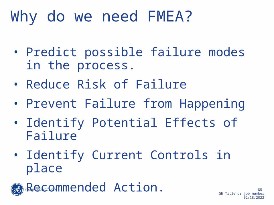
Why do we need FMEA?

• Predict possible failure modes in the process.

• Reduce Risk of Failure• Prevent Failure from Happening• Identify Potential Effects of Failure• Identify Current Controls in place• Recommended Action.

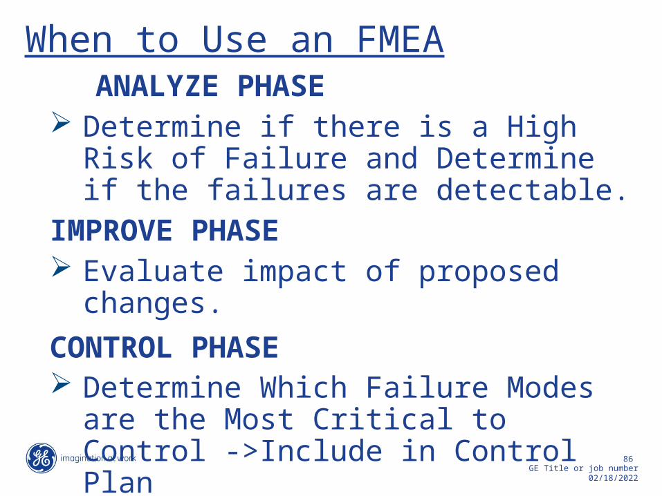
When to Use an FMEA ANALYZE PHASE Determine if there is a High Risk of

Failure and Determine if the failures are detectable.

IMPROVE PHASE Evaluate impact of proposed

changes.CONTROL PHASE Determine Which Failure Modes are

the Most Critical to Control ->Include in Control Plan

Who willDo it?

Type of Operational Measurement Data Tags Needed Data Collection Person(s) What? Where? When? How Many?Measure Measure Definition or Test Method to Stratify the Data Method Assigned

Name of X or Y Clear definition of Visual Data tags are Manual? State What Location How The numberparameter attribute or the measurement inspection defined for the Spreadsheet? who has measure is for often of data

or condition discrete defined in such a or automated measure. Such Computer based? the being data the points to be data, way as to achieve test? as: time, date, etc. responsibility? collected collection data collected

measured product or repeatable results Test instruments location, tester, is per sampleprocess from multiple are defined. line, customer, collected

data observers buyer, operator,Procedures for etc.data collectionare defined.

Define What to Measure Define How to Measure Sample PlanData Collection Plan

Measurement Systems AnalysisWhere does variation come from?

Measurement Variation

Actual Value

Measured ValueVariation

Measuring Process

The Process:Variable Data

Operators

The Tool

Part To BeMeasured

Measurements

Gage R & R Studies

• Measures the Repeatability and Reproducibility of your measurement process and compares it to the variation occurring in your part

• Or stated another way, Measures the amount of error introduced in the measurement process

Total Variation in Measurement:Preferred

Actual Variation in Product

Operator

Environment

Gage

Process

Total Variation in Measurement:Unacceptable

Actual Variation in Product

Operator

Environment

Gage

Process

Accuracy and Precision

Accuracy: How close to the measured.Precision: How repeatableExamples of:• Poor accuracy

and precision• Good precision,

poor accuracy

ActualValue

MeasuredValue

Accuracy

Repeatability(Precision)

Target Practice How could the green

player improve performance?

How could the yellow player improve performance?

Which player do you think has a better chance of becoming a champion dart player?

Typically, it is easier to shift the average than to reduce variation

Understanding Accuracy and Precision

Target

Target Target

TargetHigh accuracy & high precision Low accuracy & high precision

High accuracy & low precision Low accuracy & low precision

Gage R&R Example

• One gage• Two operators• Measuring the length of a part in

meters twice• Blind samples• Spec Limit: +/- 0.1 mm• Gage Tolerance +/-0.0001 mm

The Data

Use Minitab

Open Minitab, enter data as shownQuality Tools: Gage R&R (Crossed)Follow directions as on following sheetsMinitab uses ANOVA to perform analysis • ANOVA was discussed in DOE Class

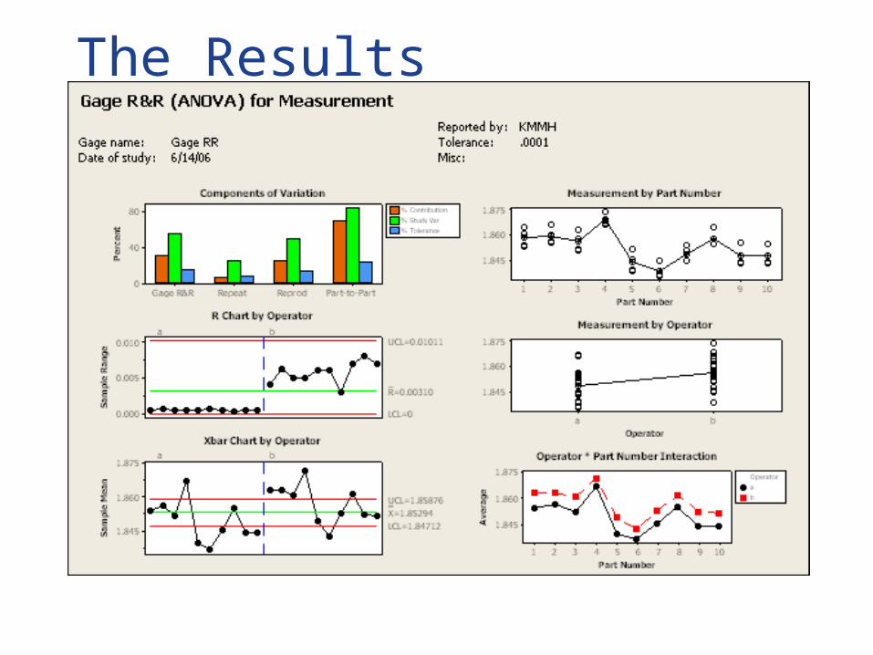
The Results

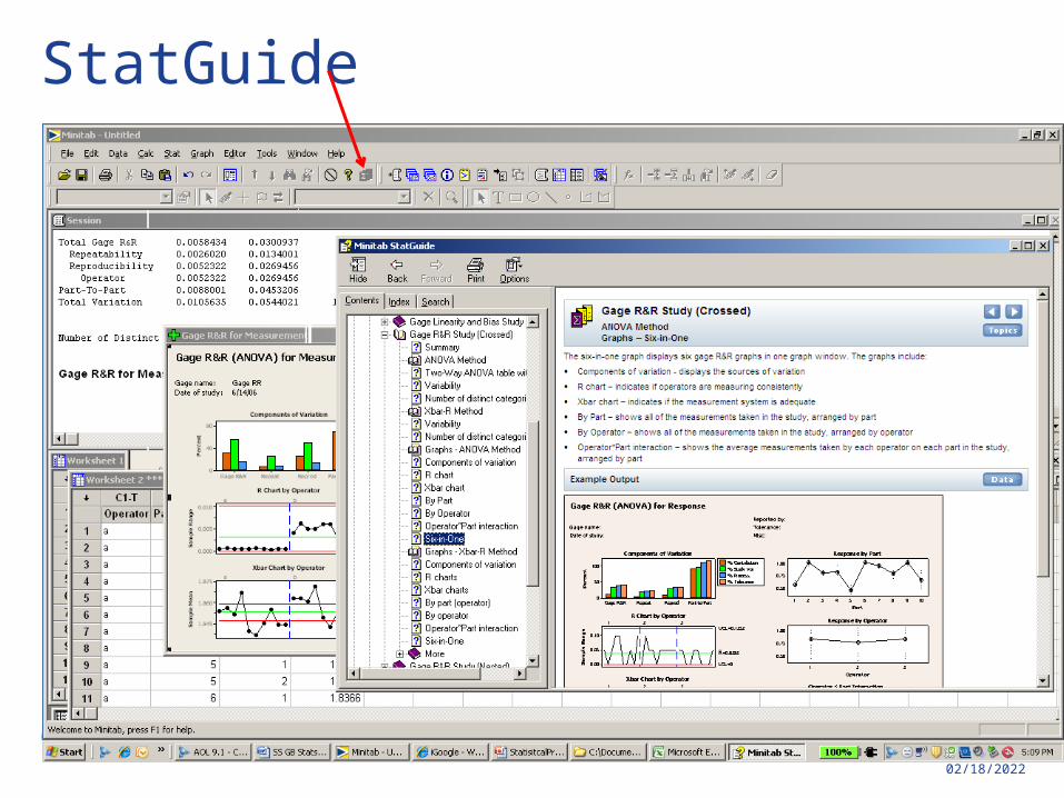
StatGuide

Statistical Process Control (SPC) is a technique that enables the quality controller to monitor, analyze, predict, control, and improve a production process through control charts.

Control charts were developed as a monitoring tool for SPC by Shewhart.

Statistical Process Control

Understanding Variation

The 6 Ms – all variation is from one or more of the 6Ms.• Man (generic)• Machine• Material• Method• Measurement• Mother nature

USLLSL

USLLSL

LSL USL

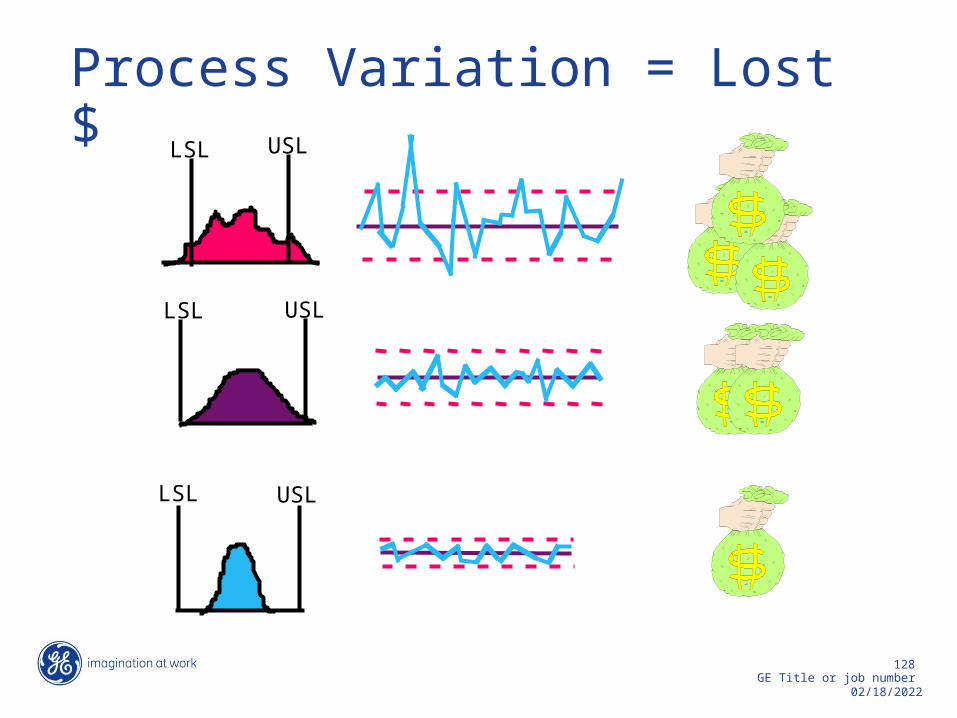
Process Variation = Lost $

Common Cause Variation

• Natural, expected variation, Controllable• Characterized by a stable and consistent pattern of variation

over time. A process operating with controlled variation has an outcome that is predictable within the bounds of the control limits.

Special Cause Variation

• Unnatural, not expected• Perform root cause analysis and eliminate if possible

Remember!

According to Deming:

85% to 95% of all variation is Common Cause.

5% to 15% of all variation is Special Cause.

“Eighty-five percent of the reasons for failure to meet customer expectations are related to deficiencies in systems and process…rather than the employee.

The role of management is to (fundamentally) change the process rather than badgering individuals to do better.”

Should We Be Concerned with Common Cause Variation?

– W. Edwards Deming

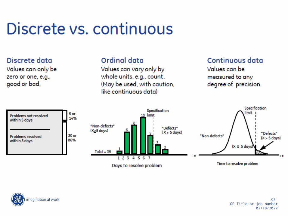
Types of DataDiscrete Data• Is Counted• Can only take certain values• Example: The number of students in class (you

cannot have a half student)

Continuous Data• Is measured• Can take any value (within a range)• Often involve fractions or decimals.• Example: A person’s height, Time (hour, minutes,

seconds), weight, length.

Control Charts• Control charts are simple but very powerful tools

that can help you determine whether a process is in control (meaning it has only random, normal variation) or out of control (meaning it shows unusual variation, probably due to a "special cause").

• Control charts have two general uses in an improvement project. The most common application is as a tool to monitor process stability and control. A less common, although some might argue more powerful, use of control charts is as an analysis tool.

Choosing Control Chart using Minitab

Commonly used Control Charts

Control Charts for Continuous DataXbar-R Charts• Xbar charts give the average value each operator obtained per

part.• R chart shows the difference between the largest and the

smallest measurement for each part. The R chart is used to evaluate the consistency of process variation. 

• Each subgroup is a snapshot of the process at a given point in time. The chart’s x-axes are time based, so that the chart shows a history of the process. For this reason, it is important that the data is in time-order.

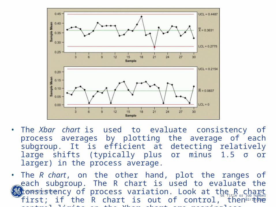
• The Xbar chart is used to evaluate consistency of process averages by plotting the average of each subgroup. It is efficient at detecting relatively large shifts (typically plus or minus 1.5 σ or larger) in the process average.

• The R chart, on the other hand, plot the ranges of each subgroup. The R chart is used to evaluate the consistency of process variation. Look at the R chart first; if the R chart is out of control, then the control limits on the Xbar chart are meaningless.

Control Charts for Discrete Data

C Charts• Assumes a Poisson distribution (counting or

integers)• Tracks the # defects and presence of Special Causes• Used when identifying the total count of defects per

unit (c) that occurred during the sampling period, the c-chart allows the practitioner to assign each sample more than one defect. This chart is used when the number of samples of each sampling period is essentially the same.

• This chart is used when the number of samples of each sampling period is essentially the same.

Control Limits

The data determine the control limits with Common Cause variation

UCL

LCL

Ave

Measurement Number

Valu

e

Control Limits Differentiate CC and SC Variation

LCL

Special Cause Variation

UCL

When a process is stable and in control, it displays common cause variation, variation that is inherent to the process.

If the process is unstable, the process displays special cause variation, non-random variation from external factors.

X bar Control Chart for SPC

Sigma 3

Sigma 2

Sigma 1

Sigma 1

Sigma 2

Sigma 3

UCL

LCL

Centerline = Mean

USL

LSL

X bar R Chart - The X bar Part

S1 S2 S3 S4 S5 S6 S7 S8 S9S10 S11 S12 S13 S14 S15 S16 S17 S18 S19 S20 S21 S22 S23 S24 S25

73.980

73.985

73.990

73.995

74.000

74.005

74.010

74.015

74.020

UCL 74.015

CL 74.001

LCL 73.988

X bar Observations

Date/Time/Period

CL = Center Line; this is the average of the averages (grand average) of each sample

aver

age

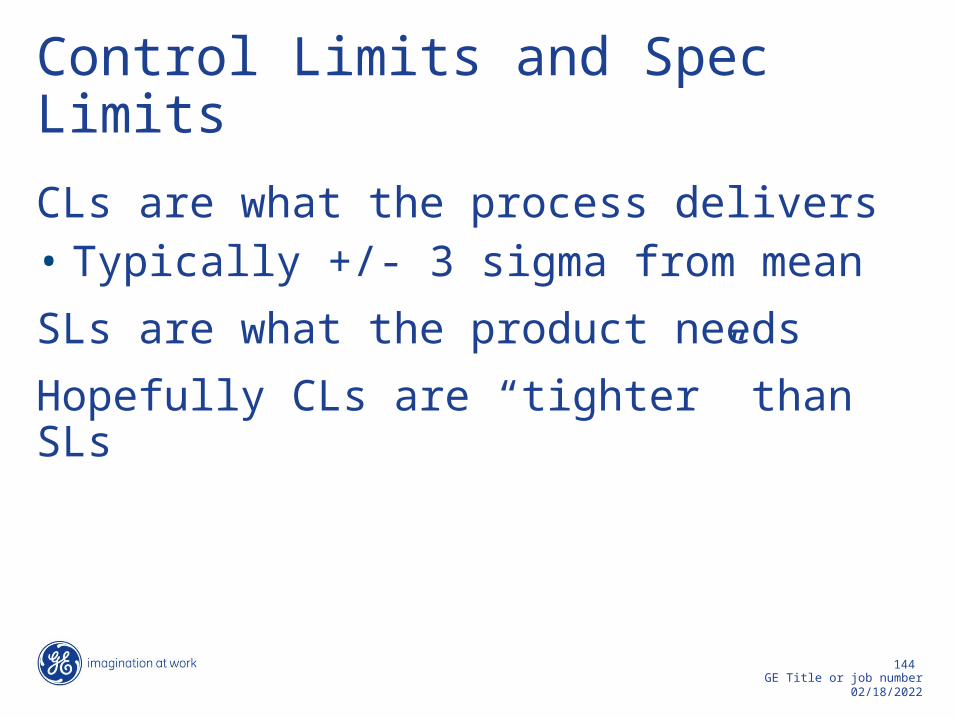
Control Limits and Spec Limits

CLs are what the process delivers• Typically +/- 3 sigma from meanSLs are what the product needsHopefully CLs are “tighter” than SLs

Sigma 3

Sigma 2

Sigma 1

Sigma 1

Sigma 2

Sigma 3

UCL

LCL

Mean

Shewhart RulesDeveloped by Dr. Walter Shewhart in 1931Assume Normal Distribution“3 sigma significant”

1891-1967

Sigma 3

Sigma 2

Sigma 1

Sigma 1

Sigma 2

Sigma 3

UCL

LCL

Mean

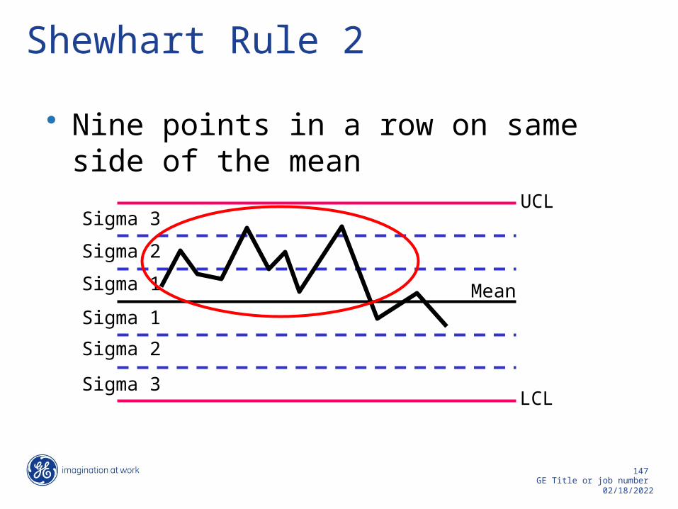
Shewhart Rule 1

• One point more than 3 sigma from mean

Sigma 3

Sigma 2

Sigma 1

Sigma 1

Sigma 2

Sigma 3

UCL

LCL

Mean

Shewhart Rule 2• Nine points in a row on same side of the

mean

Sigma 3

Sigma 2

Sigma 1

Sigma 1

Sigma 2

Sigma 3

UCL

LCL

Mean

Shewhart Rule 3• Six points in a row all decreasing or all

increasing

Sigma 3

Sigma 2

Sigma 1

Sigma 1

Sigma 2

Sigma 3

UCL

LCL

Mean

Shewhart Rule 4

• Fourteen points in a row alternating up and down

Sigma 3

Sigma 2

Sigma 1

Sigma 1

Sigma 2

Sigma 3

UCL

LCL

Mean

Shewhart Rule 5

• Two out of three points more than two sigma from the mean on the same side

Sigma 3

Sigma 2

Sigma 1

Sigma 1

Sigma 2

Sigma 3

UCL

LCL

Mean

Shewhart Rule 6• Four out of five points more than one

sigma from the mean on the same side

Sigma 3

Sigma 2

Sigma 1

Sigma 1

Sigma 2

Sigma 3

UCL

LCL

Mean

Shewhart Rule 7

• Fifteen points in a row within one sigma of mean on either side

Sigma 3

Sigma 2

Sigma 1

Sigma 1

Sigma 2

Sigma 3

UCL

LCL

Mean

Shewhart Rule 8• Eight points in a row more than one

sigma from mean on either side

Using the Rules

Xbar-R charts use 1-8 C Charts 1-4Often people will select which rules to chose, 7 and 8 are least often usedSince 3 sigma is 99.7%, if you analyze large quantities of data you will get rule violations even with CC variation

The Control Chart

Sigma 3

Sigma 2

Sigma 1

Sigma 1

Sigma 2

Sigma 3

UCL

LCL

Mean x

x

x + A2R

- A2R

Example

Stencil Printing VolumeSubgroup size =5 60 subgroupsDevelop Xbar - Chart

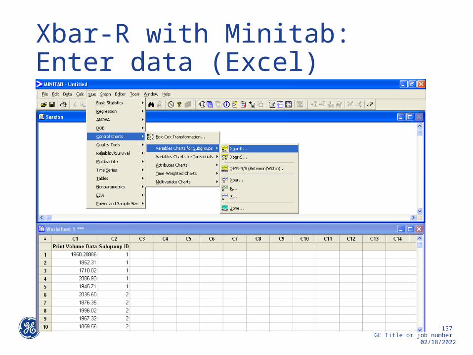
Xbar-R with Minitab:Enter data (Excel) then…..

Discussion?

Sample

Sam

ple

Mea

n

554943373125191371

2000

1900

1800

1700

__X=1870.6

UCL=2007.3

LCL=1733.9

Sample

Sam

ple

Rang

e

554943373125191371

600

450

300

150

0

_R=237.0

UCL=501.1

LCL=0

6

1

Xbar-R Chart of Print Volume Data

Stencil Printing Process

The Process:Variable Data

Process Parameters:Print SpeedSnap OffDownstop

Design:PWB LayoutStencil DesignSolder Paste Design

Materials:PWB Solder PasteStencilSqueegee

The Product:An Acceptable Board For Component PlacementQuality Level(Attribute Data)

C Charts: Control Charts for Attribute Data

Measure attribute dataEx: X defects per 1000 partsCan be done manually

xxLCL 3

xxUCL 3

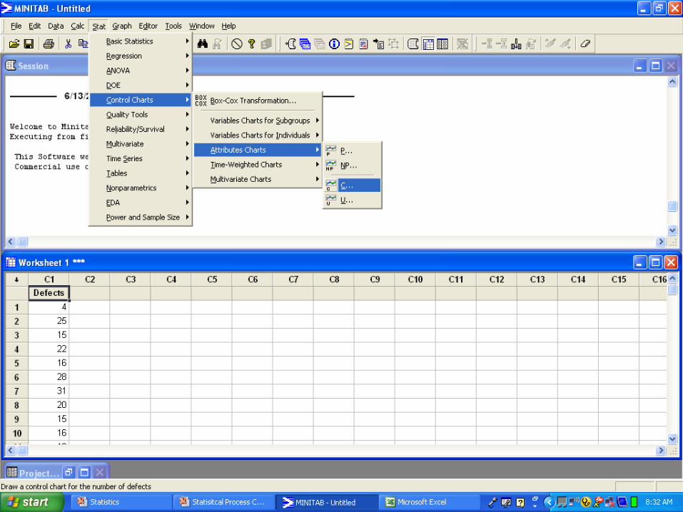
Using Minitab1. Enter defect data in column C-12. Then perform operations as above

Conclusions?

Sample

Sam

ple

Coun

t

28252219161310741

35

30

25

20

15

10

5

0

_C=13.66

UCL=24.74

LCL=2.5711

1

1

2

1

1

1

C Chart of Defects

Analysis

Other Control Charts

C and Xbar-R charts are most commonly used in SPC

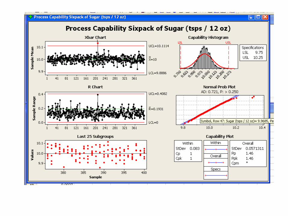
Process Capability Analysis

Where specs and process capability face off• Use Capability Sixpack (normal)• Assumes Normal DistributionIs your process in spec?How well is it in spec?• Cp• Cpk

When the Data are Not Normal

Control chart theory will be misleadingMinitab tests for normalityFortunately, data are often normal, or can be normalized with a transformation

X 1 2 3123

Mean

Capability Analysis:What are Cp and Cpk?

Cp – Process Capability ->measures precision only.Cp - is a measurement that considers the spread of the data relative to the specification limits. As shown in the following figure, a high Cp value indicates low process variation.

6 sigma means Cp = 2

Cpk – Process Capability Index ->measures precision and accuracy.

Cpk - is a measurement that considers both the spread of the data and the shift of the data relative to the specification. As shown in the following figure, a process may have good Cp but not meeting specifications (low Cpk).

6 sigma means Cp = 2 and Cpk =1.5

Remember!It is important to note that capability indices are only useful when the process is stable.

In addition, like all other statistical procedures, capability indices are only estimates based on the samples collected.

Thus, control charts are often used in conjunction to monitor the process over time rather than relying on a single number.

Good Cp and Cpk

X 1 2 3123

Mean,

99.74% with +/- 3 sigma

LSL USL

Tolerance

Width of Distribution

Good Cp, Poor Cpk

X 1 2 3123

Median, Mean, Mode

LSL USL

Width of Distribution

3 standard deviations

Cp and Cpk

• Cp = USL – LSL 6

• Cpu = USL – Xbar 3

• Cpl = Xbar - LSL

3• Cpk = min (Cpu, Cpl )

What is the Cp and Cpk of this Distribution?

X 1 2 3123

Median, Mean, Mode

99.74%

LSL USL

Tolerance

Width of Distribution

Cpl

Cpu

3 standard deviations

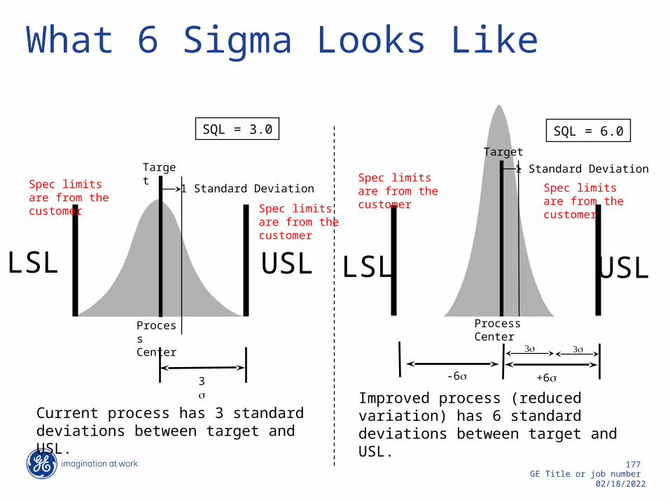
Current process has 3 standard deviations between target and USL.

USLLSL

1 Standard Deviation

Target

Process Center

3

Improved process (reduced variation) has 6 standard deviations between target and USL.

What 6 Sigma Looks Like

USLLSL

Target

Process Center

1 Standard Deviation

3

+6

3

SQL = 3.0 SQL = 6.0

-6

Spec limits are from the customer Spec limits

are from the customer

Spec limits are from the customer

Spec limits are from the customer

X

X

10 LSL

15 20 USL

10 LSL

20 USL

18

X

X

USL 10

LSL 16 20

10 LSL

15 20 USL

For σ = 1.66

For Cpk = 4

What are Cp, Cpk or σ?

For Cp = 2.5

For σ = 1

Sugar Concentration in Soda

A manufacturer wants the sugar concentration in his soft drink to be 10 teaspoons +/- 0.25 at a 3 sigma level in a 12 oz canAnalyze the data with the Capability SixpackComment on the results

Introduction to DOEsand Regression

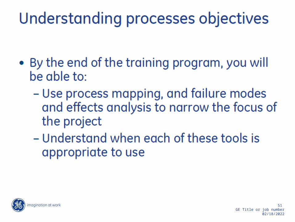
Objectives

DOE = Design of Experiment To be able to set up, solve and analyze

simple DOEs Perform simple Regression analysis

ExperimentsThe experimental method is the foundation of science and engineering• Without it we would live short, savage livesThey are a new invention• Only practiced consistently since GalileoAristotle could have avoided the mistake of thinking that women have fewer teeth than men, by the simple device of asking Mrs. Aristotle to keep her mouth open while he counted. ---Bertrand Russell

What is DOE?Most processes are affected by multiple factors• Example: Stencil Printing• Factors: Stencil, paste, snap off speed, print speed,

wipe frequencyWith DOE, the effect of all the factors can be determined with a minimum amount of testing• The results are “statistically significant,” not an

opinionThe old way: one experiment for each factor => not effective• Requires much more data, interactions are a

problem

History

1830 – Gauss• Curve fitting with least squares • The “Normal” or “Gaussian” Curve1908 – “Student” develops t -Test to analyze beer1920 - DOE Concepts Developed• First in Agriculture….calculations harder than experiments1950-80s “Taguchi” Developed1951 - Central Composite Design1990’s - D optimal designs• Experiments harder than calculations

DOE: Step 1

Clarifying the process mechanisms is crucialHence, have a brainstorming session to identifying independent variables (factors)

Guidelines for Brainstorming

Team Makeup• Experts• “Semi” experts• Implementers• Analysts• Technical Staff who will run the

experiment• Operators

Guidelines for Brainstorming

Discussion Rules• Suspend judgement• Strive for quantity• Generate wild ideas• Build on ideas of others

Guidelines for Brainstorming

Leader’s Rules for Brainstorming• Be enthusiastic• Capture all ideas• Make sure you have a good skills mix• Push for quantity• Strictly enforce the rules• Keep intensity high• Get participation from everybody

Conducting a DOE Steps 1 through 5

1. State the Problem2. Define the Objective3. Set the start and end dates4. Select the Response

– e.g., Solder paste volume5. Select the factors

– e.g., Print Speed, Separation Speed, Paste, Stencil, etc.

6. Define the team and resources7. Select design type

– e.g., Full factorial, etc.8. Conduct experiment9. Analyze data10. Plan and execute further tests from

these results

Conducting a DOE Steps 6 through 10

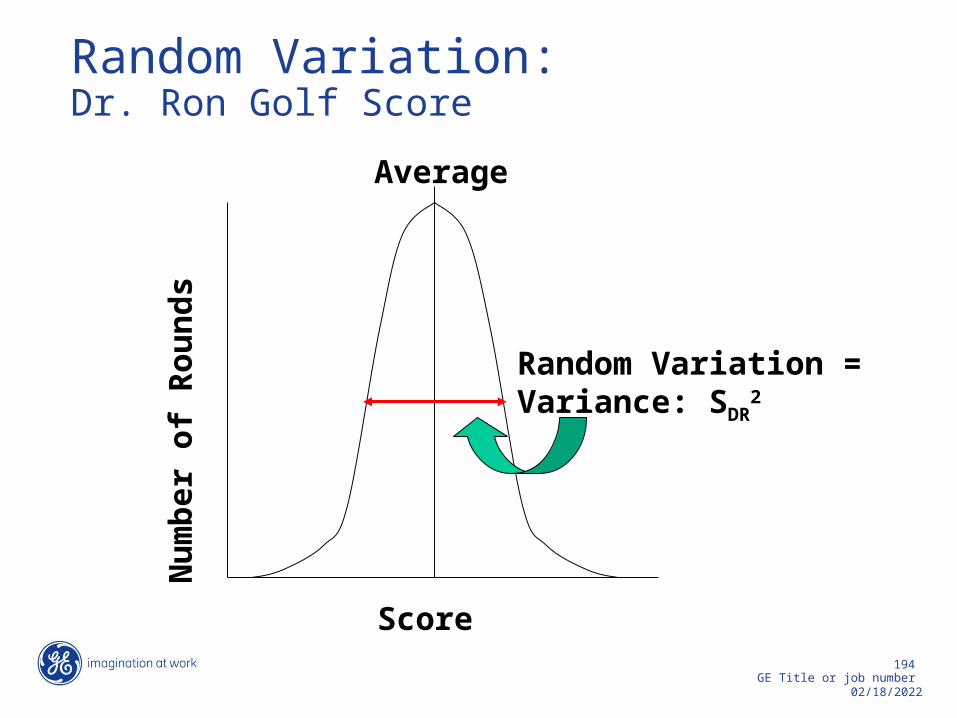
Score

Random Variation =Variance: SDR

2

AverageN

umbe

r of R

ound

s

Random Variation:Dr. Ron Golf Score

Tiger Dr. Ron Score

D Differencein averages

Implies that there is a greater difference between Tiger and Dr. Ron than among them D2 >> Sr

2

Num

ber o

f Rou

nds

STiger2

Variation from Factors: Tiger and Dr. Ron

SDR2

For example: Phil Mickelson and Steve Stricker. Then, D2 << Sr

2

D

Mul

tiple

Rou

nds

Golf Score

Sr2

When Variation from Factor Change is Small…….

ANOVA

ANOVA (Analysis of Variance)• Compares S2

to D2

The F Statistic:

Large F => factors have a significant effect on result“Large” varies with sample size, typically > 4 for 95% confidence

2

2

rSF D

The Null Hypothesis

H0: The mean response at two different factor levels is the same.Example: The Tiger and Dr. Ron score the same.Typically, we want to see if we can reject H0 at a certain “level of confidence” F ~ 4 can reject H0 with >95% confidence:• P<0.05

DOE SizeThe amount of data needed quickly grows with the number of factors and levelsF = number of factors, L= number of levelsData Points = LF

• a 6 factor, 4 level experiment = 4096 data points

DOE Size

Must work to minimize # of factors and levels“If it’s too big, it won’t get done.” - Joe BelmonteFractional factorial, Taguchi, Plackett-Burman, and D-Optimal Designs were created to minimize data collectionBut, always with the loss of something

DOE Example and TheoryApple growthTwo Factors: Water and fertilizer are believed to increase the quantity of apples. It is not known if there are interactions between the two factorsTwo Levels: For each FactorResponse: Crates of ApplesWe will do a “full factorial” experiment

The DataRun Water

(A) Fertilizer

(B) Resp1 (100 crates)

Resp2

1 70 100 2.2 2.8

2 70 200 3.2 3.6

3 90 100 5.0 4.6

4 90 200 5.8 5.4

Parallel lines => No Interaction!

Apple Production vs Amount of Irrigation

0

1

2

3

4

5

6

60 65 70 75 80 85 90 95

Units of Water

Appl

es (

100

Crat

es/t

ree)

200 Units Fertilizer

100 Units Fertilizer

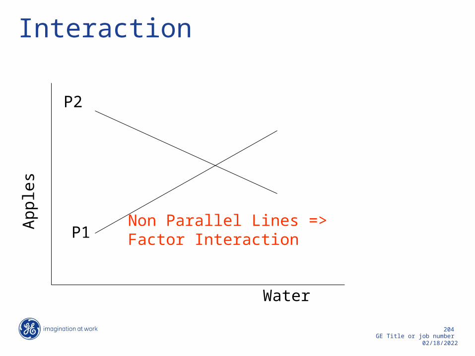
Interaction

Water

App

les

P1

P2

Non Parallel Lines => Factor Interaction

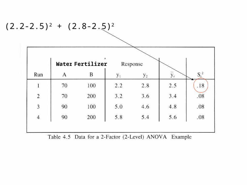
(2.2-2.5)2 + (2.8-2.5)2

Water Fertilizer

Number of responses minus 1

Cross Product Term

If we reject Ho

we are wrongonly 5% of the time.

(4.8+5.6)/2 -(3.4+2.5)/2

Still can reject strongly H0

Cross product term not significant

Strong A and B dependence, weak AxB

What does ANOVA Do?

ANOVA uses the analysis of variance to determine if the “treatment” is more significant than random error

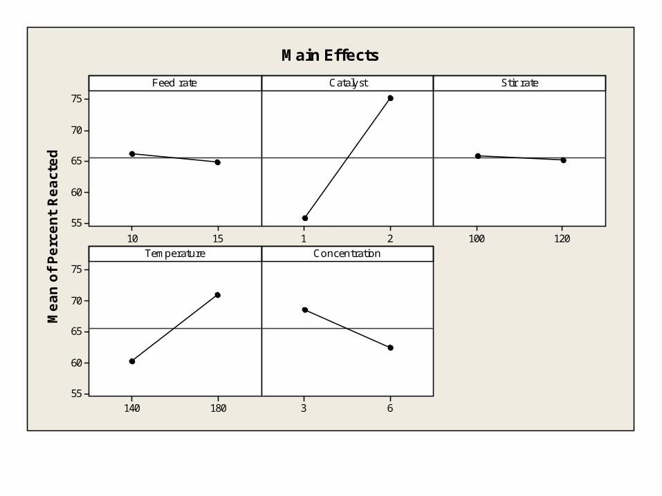
Factors in a Chemical Reaction

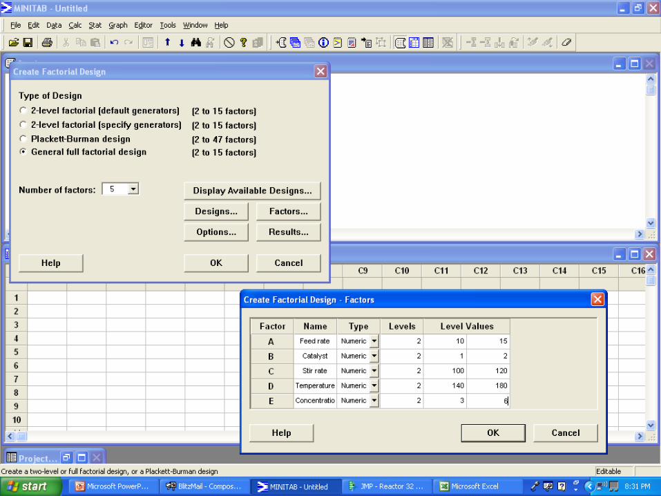
Feed rate, Catalyst, Stir rate, Temperature and Concentration are to be evaluated on their effect to increase the percent reactedTwo levels for each factor are considered:• Feed rate: 10, 15 (g/min)• Catalyst: 1, 2• Stir rate: 100,120 (stirs/min)• Temperature: 140, 180 (degrees F)• Concentration: 3, 6 (g/L)

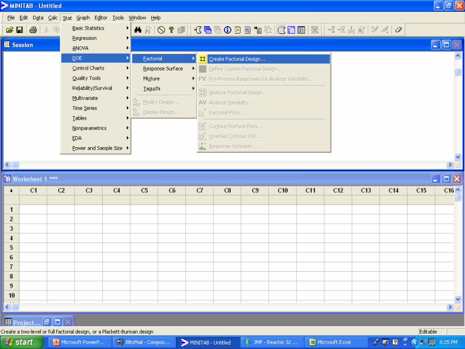
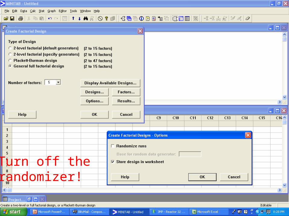
Turn off the randomizer!

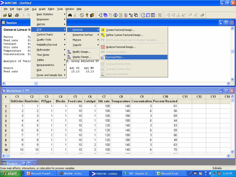
Now Paste in your Data

Note: If you only have one replicate, do not select more than a 2nd order fit

Mea

n of

Per

cent

Rea

cted

1510

75

70

65

60

5521 120100

180140

75

70

65

60

5563

Feed rate Catalyst Stir rate

Temperature Concentration

Main Effects

Feed rate

21 120100 180140 6390

75

60

Catalyst

90

75

60

Stir rate

90

75

60

Temperature

90

75

60

Concentration

1015

rateFeed

12

Catalyst

100120

Stir rate

140180

Temperature

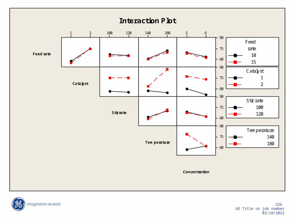
Interaction Plot

But Always…..

Look at the raw data

DOE Class Problem: using Minitab on your ownThree new additives are being pursued to increase

stainless steel cutlery hardness. Each additive (A,B,C) is tested at four levels. In addition, two new cold quench temperatures are tried. The data are “Stainless DOE/Regression.”Use DOE techniques (Full Factorial, turn randomizer off, 1 replicate, select 2nd order) to determine which additives have an effect on the hardness and whether quench temperature is important. Using factorial plots, comment on the results. What formulation and treatment would you suggest from these data to maximize hardness? What future experiments might you want to do to learn more about hardness as a function of the factors?

Don’t jump ahead, answers are on the next slide!

Analysis of Variance for Rockwell C Hardness, using Adjusted SS for Tests

Source DF Seq SS Adj SS Adj MS F PA 3 18.141 18.141 6.0471 682.78 0.000B 3 38.567 38.567 12.8555 1451.5 0.000C 3 12.227 12.227 4.0755 460.17 0.000Quench Temp 1 0.0021 0.0021 0.0021 0.24 0.626A*B 9 0.1127 0.1127 0.0125 1.41 0.196A*C 9 0.0516 0.0516 0.0057 0.65 0.754A*Quench Temp 3 0.0220 0.0220 0.0073 0.83 0.483B*C 9 0.0708 0.0708 0.0079 0.89 0.540B*Quench Temp 3 0.0052 0.0052 0.0017 0.20 0.899C*Quench Temp 3 0.0066 0.0066 0.0022 0.25 0.862Error 81 0.7174 0.7174 0.0089Total 127 69.9228

S = 0.0941094 R-Sq = 98.97% R-Sq(adj) = 98.39%

Session Window Conclusions:

Additives A, B & C are statistically significant. Need to find optimal level to achieve specified hardness. Quench temperature and interactions not statistically significant.

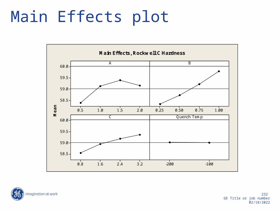
Main Effects plot

2.01.51.00.5

60.0

59.5

59.0

58.5

1.000.750.500.25

3.22.41.60.8

60.0

59.5

59.0

58.5

-100-200

AM

ean

B

C Quench Temp

Main Effects, Rockwell C Hardness

Main Effects Conclusions

Additive A achieves optimal hardness between 1.0 & 2.0. Further experimentation with greater resolution between these points recommended.• If cost prohibits, can recommend to use

level 1.5, as this produces the hardest steel of levels tested

Additives B & C do not achieve any local or global optimum. Further experimentation at higher dosages recommended• Or if costs prohibit, use the highest

levelsQuench temp is not statistically significant.• Can choose to use level that is

cheaper• This information is just as important

because it allows the business to do what is cheaper.

Interaction Plot

1.000.750.500.25 3.22.41.60.8 -100-200

60

59

58

60

59

58

60

59

58

A

B

C

Quench Temp

0.51.01.52.0

A

0.250.500.751.00

B

0.81.62.43.2

C

Interaction Plot - Rockwell C Hardness

Interactions discussion

No interactions statistically significant.• Seen previously in your session window• Seen here as there are no non-parallel

lines

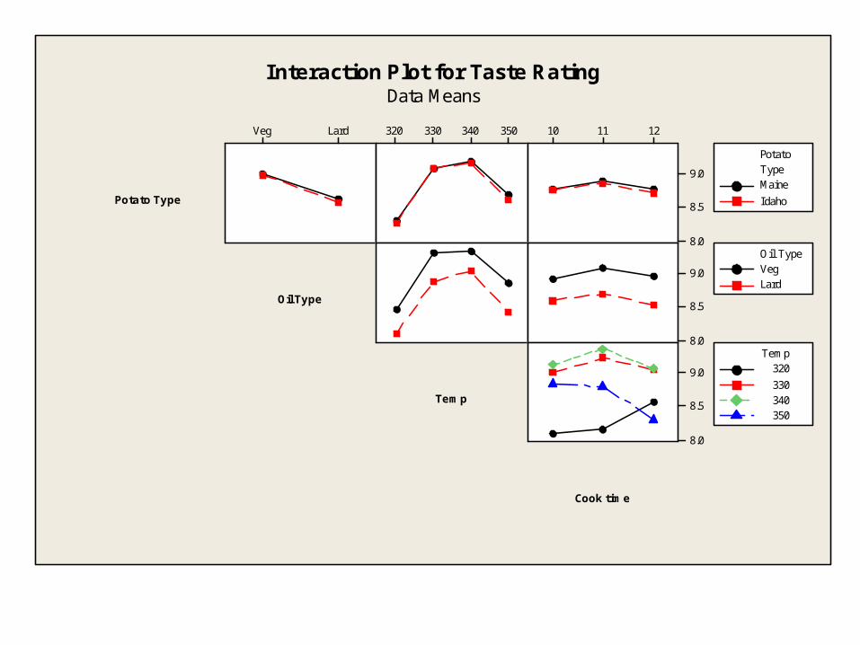
Extra Problem: French Fries

McDonalds is concerned that their French fries are losing favor to Burger King. They perform a DOE to optimize taste. Professional testers evaluate the taste of the fries that have been cooked under varying conditions. The average of 10 tasters is the “response.” Ten is the best rating, one is the worst. The experiments are performed twice to get two replicates of data. The factors are: Potato Type: Maine or Idaho, Cooking Oil Type: lard or vegetable, cooking temperature: 320, 330, 340, 350oF and cooking time 10, 11 or 12 minutes. The results are in the spreadsheet in tab “French Fry DOE”. Historically, lard has made better tasting fries, but the vegetable oil is a new version, specifically designed for improved taste.Analyze and discuss.

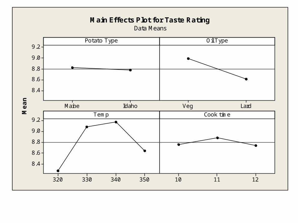
IdahoMaine

9.29.08.88.68.4

LardVeg

350340330320

9.29.08.88.68.4

121110

Potato Type

Mea

n

Oil Type

Temp Cook time

Main Effects Plot for Taste RatingData Means

LardVeg 350340330320 121110

9.0

8.5

8.0

9.0

8.5

8.0

9.0

8.5

8.0

Potato Type

Oil Type

Temp

Cook time

MaineIdaho

TypePotato

VegLard

Oil Type

320330340350

Temp

Interaction Plot for Taste RatingData Means

Improvement

Tool Overview

*It is not expected that all tools be used – the project focus and questions must drive the tool selection.

Define Measure Analyze Improve Control KaizenRACIStakeholder AnalysisNorms/Ground RulesSIPOCBaseline MeasurementsContractProject PlanReview Process Cost Benefit Analysis

Integrated Flowchart8 Types of WastePareto DiagramKano ModelCustomer /Results MatrixResults/Process MatrixOperational DefinitionsSampling PlanData Collection FormMeasurement AnalysisControl ChartProcess CapabilityDPMOHistogramRun ChartsCause and Effect Diagram

Pareto DiagramAffinity DiagramInterrelationship DiagraphControl ChartScatter DiagramPareto DiagramStratificationHypothesis TestingRegression AnalysisTree DiagramDesign of ExperimentCube PlotPDSA Test Plans

BrainstormingLateral Thinking5SSolution and Effect DiagramImplementation PlanGantt ChartFlow Chart (To Be)Control ChartParetoVisual ManagementLine BalancingPoke-YokeFMEA

Arrow DiagramGantt ChartRisk AssessmentStakeholder AnalysisCommunication PlanSOPControl ChartControl PlanTraining PlanForce Field AnalysisCost Benefit AnalysisFinal Project Review DocumentSuccess Story for Publication

Review ProcessCommunication Plan

Key Tools / Techniques Typically Used in Each Phase