K.7

Learning in the Oil Futures Markets: Evidence and Macroeconomic Implications Leduc, Sylvain, Kevin Moran and Robert J. Vigfusson

International Finance Discussion Papers Board of Governors of the Federal Reserve System

Number 1179 September 2016

Please cite paper as: Leduc, Sylvain, Kevin Moran and Robert J. Vigfusson (2016). Learning in the Oil Futures Markets: Evidence and Macroeconomic Implications. International Finance DiscussionPapers 1179. http://dx.doi.org/10.17016/IFDP.2016.1179

Board of Governors of the Federal Reserve System

International Finance Discussion Papers

Number 1179

September 2016

Learning in the Oil Futures Markets: Evidence and Macroeconomic Implications

Sylvain Leduc, Kevin Moran, and Robert J. Vigfusson

NOTE: International Finance Discussion Papers are preliminary materials circulated to stimulate discussion and critical comment. References in publications to International Finance Discussion Papers (other than an acknowledgment that the writer has had access to unpublished material) should be cleared with the author or authors. Recent IFDPs are available on the Web at www.federalreserve.gov/pubs/ifdp/. This paper can be downloaded without charge from Social Science Research Network electronic library at http://www.ssrn.com/.

Learning in the Oil Futures Markets: Evidence and

Macroeconomic Implications

Sylvain Leduc

Bank of Canada

Kevin Moran

Universite Laval

Robert J. Vigfusson∗†

Federal Reserve Board

Abstract

We show that a model where investors learn about the persistence of oil-price

movements accounts well for the fluctuations in oil-price futures since the late

1990s. Using a DSGE model, we then show that this learning process alters the

impact of oil shocks, making it time-dependent and consistent with the muted

impact oil-price changes had on macroeconomic outcomes during the early 2000s

and again over the past two years. The Spring 2008 increase in oil prices had a

larger impact because market participants considered that it was likely driven by

permanent shocks.

JEL Codes: E32, E37 , Q43

Keywords: Kalman filter, time-variation, inventories, conditional response

∗The views in this paper are solely the responsibility of the authors and should not be interpreted

as reflecting the views of the Governing Council of the Bank of Canada, the Board of Governors of

the Federal Reserve System, or any other person associated with the Bank of Canada or the Federal

Reserve System.†We thank seminar participants at the Federal Reserve Board, the Federal Reserve Bank of Boston,

the Federal Reserve Bank of Cleveland, the Swiss National Bank, the Bank of Canada, Larefi (Uni-

versity of Bordeaux), and conference participants at the BI Norwegian Business School and the 2015

NBER meeting on the Economics of Commodity Markets. In particular thanks to Benjamin Johannsen,

Matt Smith, Hilde Bjornland, and Fabio Canova. Comments to robert.j.vigfusson@frb.gov.

1

1 Introduction

The large fluctuations in the price of oil over the past 15 years have renewed interest in

the usefulness of the oil futures market in anticipating future price movements (Alquist

and Kilian, 2010; Alquist, Kilian, and Vigfusson, 2013). However, the futures market

appeared to have only slowly recognized that events since the early 2000s, from the

growing importance of China in the world economy to the onset of the financial crisis

and the more recent shale revolution, would radically change the outlook for oil prices.

Whereas the resulting forecast errors over this period have often been attributed to

speculation or to time-varying risk, this paper provides an explanation of the movements

in oil-price futures based on learning and shows through a DSGE model that this

learning process has important macroeconomic implications.

In particular, our analysis indicates that the developments in the oil futures markets

since the late 1990s are largely consistent with investors learning about the persistence

of underlying shocks. Using the Kalman filter to infer the permanent and transitory

components of shocks to spot oil prices, we show that this simple form of learning can

explain the observed behavior of futures prices reasonably well. Our simple framework

accounts for the relatively slow increase in oil-price futures at the beginning of the past

decade and their unprecedented run-up between 2004 and 2008. Even during the first

half of 2008, a period during which oil prices reached historic highs, the model predicts

a level of futures prices that is broadly in line with the data. Our estimates suggest a

significant and steady increase in the variance of the permanent component of shocks

to spot oil prices from 2002 to 2008, accompanied by a similarly steady decline in the

variance of the temporary component. In turn, these varying estimates translate into a

growing contribution of permanent shocks to the variance of oil prices over this period.

More recently, our analysis indicates that investors largely perceived the drop in oil

prices during the second half of 2014 as being transitory.1

1Although the Kalman filter has the advantage of being a straightforward approach to model learn-

ing, it is also somewhat restrictive since it assumes that the parameters of the model are constant. In

robustness exercises, we present results for two alternative models that allow for time-varying param-

eters: a constant-gain learning model and a variant of Stock and Watson’s unobserved components

model (2007) with stochastic volatility, with the unobserved components estimated via the particle

filter. We find that our baseline results derived using the Kalman filter are little changed under either

alternative model.

2

Our findings have important implications regarding the macroeconomic impact of oil

shocks. Using a DSGE model in which oil is storable and used in production, we show

that agents’ learning in the form suggested by our empirical results alters the effects

of oil shocks by making them time-varying. Consistent with our empirical results, we

calibrate three scenarios that capture market participants’ perceptions regarding the

persistence of oil prices: first, in 2003, when changes in oil prices were largely thought

to be transitory; next, in 2007, when oil-price changes were expected to be much more

persistent; and finally in 2014 during the recent oil-price collapse. Compared with a

framework with full information, we show that the recessionary effects of permanent oil-

price increases are roughly halved in the year following the rise in the price of oil under

the 2003 scenario. In contrast, the increase in oil prices in the spring of 2008 had a larger

impact on output, in part because market participants were more likely to view the rise

in oil prices as driven by permanent shocks than earlier in the 2000s.2 Our analysis also

indicates that the large drop in oil prices during the second half of 2014 did not translate

into a correspondingly large boost in economic activity partly because investors initially

viewed the price declines as being fairly transitory. We show that part of this dampening

effect is due to an interaction between learning and storage. In particular, believing

that the oil shock is transitory leads agents to draw down inventories, which initially

mutes the rise in oil prices and the associated fall in economic activity.

A more muted dampening effect occurs under our 2007 and 2014 scenarios. We

show that part of this dampening effect is due to an interaction between learning and

storage. In particular, believing that the oil shock is transitory leads agents to draw

down inventories, which initially mutes the rise in oil prices and the associated fall in

economic activity.

The more muted effects of permanent oil shocks under learning and storage partly

account for the relatively weak impact on growth from the run-up in oil prices in the

mid-2000s (see Blanchard and Galı, 2009). As such, our results complement Kilian’s

(2008) emphasis on the importance of the source of oil shocks in understanding their

effects on GDP. In particular, Kilian finds that the run-up in oil prices starting in 2003

was largely driven by an increase in world aggregate demand and thus had a muted

effect on U.S. economic growth. Our results indicate that the effect on growth was also

muted because market participants initially failed to correctly assess the persistence of

2Hamilton (2009) analyzes the contribution of the oil shock of 2007-08 to the Great Recession.

3

the increase in oil prices. Similarly, our model simulations are consistent with the view

that the steep decline in oil prices in the summer of 2014 did not translate into a large

boost to economic activity.

1.1 Related literature

A growing literature seeks to understand the large movements in the spot price of oil

and its changing relationship with the futures market. In particular, our paper relates

to some of the recent work on the role of financial markets in driving oil prices.3 For

instance, Hamilton and Wu (2014) argue that increased participation by index-fund

investing has reduced oil futures premiums since 2005, accounting for the smaller gap

between spot and futures prices observed in the data between 2005 and 2008. Similarly,

Buyuksahin et al. (2008) argue that increased market activity by commodity swap

dealers, hedge funds, and other financial traders, has helped link crude oil futures

prices at different maturities. Acharya et al. (2013) emphasize limits to arbitrage and

their effects on spot and futures prices in commodity markets. In their environment,

speculators face capital constraints in commodity markets, which limits commodity

producers’ ability to hedge risk and is reflected in commodity prices. As such, these

papers attribute developments in the futures markets to the increased financialization

of commodity markets or to speculators’ risk appetite, while we show that part of these

movements can be attributed to learning. Our emphasis on learning in the futures

markets is compatible with Kellog’s result (2014) that conditioning on oil futures better

explains drilling decisions than assuming that oil prices followed a random walk.

Our paper also complements the work of Alquist and Kilian (2010). They empha-

size the presence of a convenience yield associated with oil inventories and its role in

accounting for the large and persistent fluctuations in the oil futures spread. Using a

theoretical model, they argue that, under greater uncertainty about future oil supplies,

the presence of a convenience yield may underlie the poor predictive performance of oil-

price futures. We add to this literature by highlighting the interaction between learning

and oil storage.

Our approach also shares with Milani (2009) the emphasis on learning. In a DSGE

3This literature is large and growing. Some of the many papers discussing this issue include Irwin

and Sanders (2012); Fattouh, Kilian and Mahadeva (2013); Kilian and Murphy (2014); Alquist and

Gervais (2013); and Singleton (2014).

4

model in which oil is used in production, Milani (2009) studies the effect of learning

on the changing relationship between oil prices and the macroeconomy since the 1970s,

assuming that agents in the model learn about the parameters of the model and the

underlying shocks through constant-gain learning. He shows that learning is important

to account for the changing effects of oil shocks on output and inflation over time.

In contrast, our approach highlights that the futures markets also provide valuable

information about the learning process. We show that a simple model of learning about

the persistence of underlying shocks tracks the evolution of oil futures prices since the

late 1990s reasonably well, and that this type of learning can alter the impact of oil

shocks on the macroeconomy. Our work on showing the importance of learning in a

DSGE model and its implications for economic outcomes is also related to work by

Slobodyan and Wouters (2012), Fornero and Kirchner (2014) and Ormeno and Molnar

(2015).

Lastly, throughout our analysis we focus on the role of learning, abstracting from

other possible important factors that can also influence futures prices. For instance,

we abstract from risk-premium variations, which have been shown to be important in

understanding futures prices during particular episodes, for instance at the height of

the oil-price boom in the beginning of 2008 (see, Baumeister and Kilian, 2015).

The rest of the paper is organized as follows. After describing in more details

movements in oil prices over the past 15 years, we lay out our empirical framework,

estimating a time-series model of permanent and temporary shocks to oil prices. We

then develop a theoretical framework to examine the impact of learning about the

persistence of oil-market developments on the economy, calibrating the learning process

to match our empirical findings in 2003, 2007, and 2014. After describing our theoretical

findings, we conclude in the last section.

2 Oil prices during the 1990s, 2000s, and beyond

We start our analysis by presenting some evidence of the oil market’s evolving views

regarding the persistence of the shocks hitting the world economy. To do so, consider

the movements in the spot and futures prices of oil since the early 1990s, depicted in

the three panels of Figure 1. In each panel, the solid line shows the evolution of the

spot price, while the dotted lines depict the path of futures prices at a given point in

5

time. The futures prices are quotes as reported by NYMEX. During the 1990s (top

panel), the spot price tended to gyrate around fairly stable oil-price futures, suggesting

that market participants viewed economic developments affecting the oil market as

mainly temporary. Underlying shocks would tend to move the spot price of oil, at

times substantially, but futures prices would indicate an expected return to roughly

$18 per barrel, about the average spot price during that period. Clearly, whatever the

disturbances affecting the world economy, market participants did not view them as

persistent enough to substantially alter their long-term view of oil prices, and these

views were substantially correct during the 1990s.

However, the middle panel of Figure 1 indicates that the relationship between spot

and futures prices changed during the early 2000s. Between 2000 and 2008, the spot

price of oil rose steadily, from roughly $27 per barrel to more than $135 per barrel. In

contrast, oil-price futures remained initially low, consistently fluctuating below $20 per

barrel until 2003. Then, oil-price futures started a gradual rise, increasing to roughly

$50 per barrel by the mid-2000s. Spot and futures prices then tended to move in lockstep

between 2005 and 2008.

One possible interpretation of this pattern is that, between 2000-03, market par-

ticipants perceived movements in spot prices as likely to be temporary, as indeed was

the case throughout the 1990s. However, after being consistently surprised by the per-

sistence of the rise in spot prices, market participants reassessed their views, placing

more weight on the possibility that the increase in oil prices was persistent rather than

transitory.

According to this interpretation, by the time the oil market reached its peak in the

spring of 2008, market participants largely expected the movements in spot prices to

be highly persistent, remaining at about $135 per barrel over the next five years, as

indicated by the futures curves at that time. The graph also suggests that the global

financial crisis during the fall of 2008 led to a reassessment of the long-run equilibrium

price of oil. Indeed, the far-dated futures prices declined from roughly $140 per barrel

in the spring of 2008 to roughly $60 per barrel by the end of that year.

Lastly, the evolution of spot and futures prices since 2010 is shown in the bottom

panel of the figure. Between 2010 and 2014, the fluctuations in prices had more in

common with the 1990s. That is, market participants appear to have perceived that

most of the fluctuations in the spot price of oil were largely transitory, with the long-

run futures price remaining fairly stable despite significant movements in the spot price.

6

However, the oil market changed dramatically in mid-2014 when the spot price collapsed

by roughly 50 percent.4 As in the early 2000s, it took some time for futures markets

to change their views about the persistence of the price change, which was initially

perceived as being somewhat temporary, with futures curves rising back to a long-run

price of about $80 per barrel during most of 2014. By the end of 2015, this assessment

was substantially changed, as far-dated futures prices only reached about $55 per barrel.

3 Empirical framework

In this section, we develop a simple unobserved components model to account for the

role of permanent and temporary shocks in determining oil-price futures. By design,

we adopt a straightforward approach to highlight our main point. Accordingly, we

abstract from many features of the oil market. Specifically, we postulate that spot oil

prices are the result of movements in permanent and transitory components and that

market participants use the Kalman filter to assess the relative importance of these

two components over time. In addition, under our baseline model, we allow the model

parameters to evolve with the data sample. In Appendix A, we assess the robustness

of our baseline results by analyzing alternative models that explicitly allow for time-

varying parameters. As reported in the appendix, results are largely unchanged.

3.1 A simple model

Consider the following linear process relating the spot price of oil st (expressed in logs)

to a permanent component, ePt , and a stationary one, eτt ,

st = ePt + eτt . (1)

Schwartz and Smith (2000) modelled oil prices using this assumption but, unlike in the

current paper, they assumed that the model parameters were constant. The permanent

component is modelled as a random walk with drift:

ePt = µ+ ePt−1 + vt, (2)

4Further discussion of this decline can be found in Baumeister and Kilian (2016).

7

where vt is an independently and identically normally distributed disturbance with

mean zero and constant variance σ2p. The temporary component is assumed to follow

the AR(1) process

eτt = φτeτt−1 + εt, (3)

where εt is an independently and identically normally distributed disturbance with mean

zero and constant variance σ2τ and with |φτ | < 1.

Assuming full information at time t about the temporary and permanent components

underlying oil prices, the k-period-ahead futures price at time t, ft,k, is given by the

following expression:

ft,k = Etst+k = kµ+ ePt + φkτeτt . (4)

In contrast, absent full information about the current levels of ePt and eτt , the futures

price will be based on the best forecasts given past values of st:

ft,k = Et(st+k| {st−i}1

i=t

)= Et

(kµ+ ePt + φkτe

τt | {st−i}

1i=t

). (5)

To determine the relative importance of permanent shocks, a simple statistic can be

derived from the expression for the change in the spot price of oil:

4st = µ+ vt + (φτ − 1) eτt−1 + εt,

which implies that the variance of 4st can be expressed as

σ24s = σ2

p +2

(1 + φτ )σ2τ ,

and the fraction of σ24s due to permanent shocks is captured by the following expression:

σ2p

σ2p + 2

(1+φτ )σ2τ

.

3.2 Learning

We assume that market participants use the Kalman filter to form expectations of

future oil prices. Our treatment of the Kalman filter is a standard textbook treatment

(Hamilton, 1994). In particular, define ξt as the unobserved state vector of the model

above, comprising the trend, µ, as well as the permanent and temporary components:

ξt =(µ ePt eτt µ ePt−1 eτt−1

)′. Given values of the model’s parameters, Γ = [ σ2

p,

8

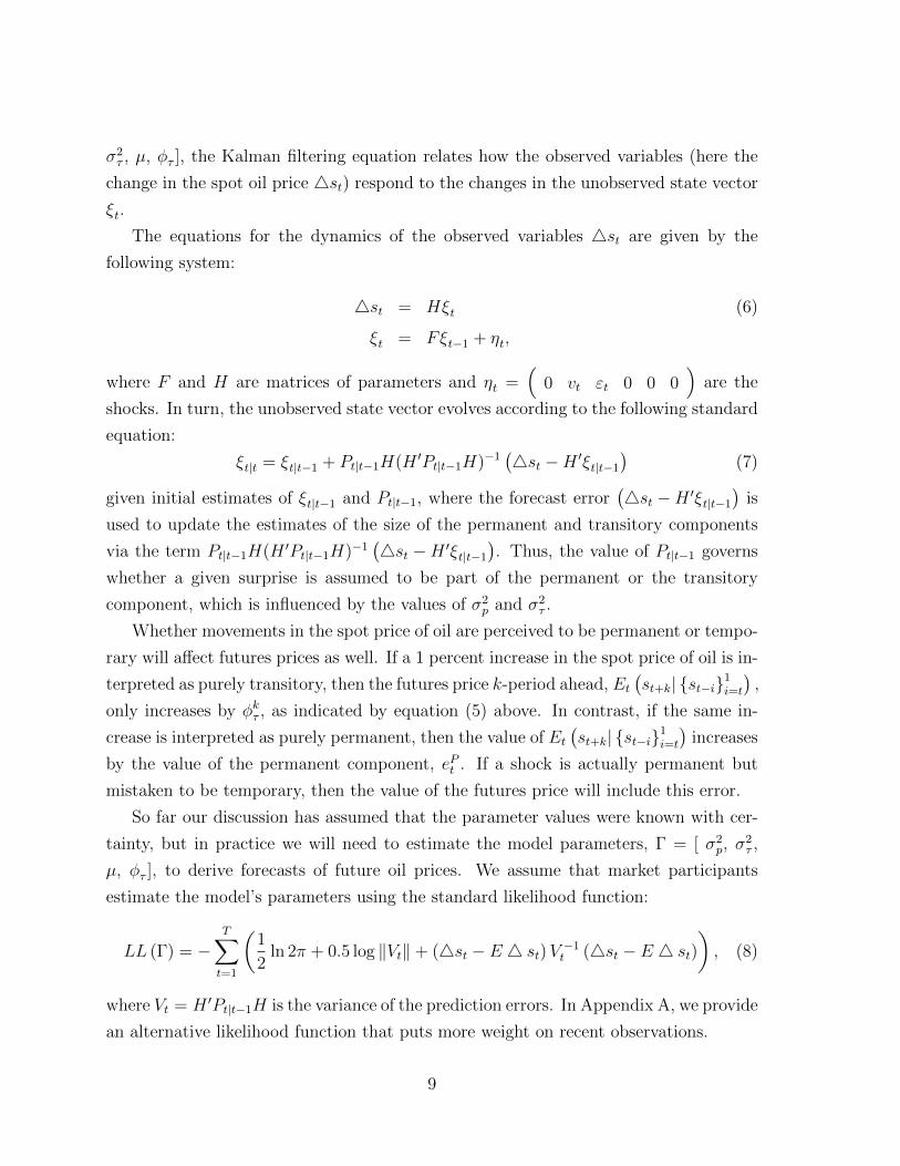
σ2τ , µ, φτ ], the Kalman filtering equation relates how the observed variables (here the

change in the spot oil price 4st) respond to the changes in the unobserved state vector

ξt.

The equations for the dynamics of the observed variables 4st are given by the

following system:

4st = Hξt (6)

ξt = Fξt−1 + ηt,

where F and H are matrices of parameters and ηt =(

0 vt εt 0 0 0)

are the

shocks. In turn, the unobserved state vector evolves according to the following standard

equation:

ξt|t = ξt|t−1 + Pt|t−1H(H ′Pt|t−1H)−1(4st −H ′ξt|t−1

)(7)

given initial estimates of ξt|t−1 and Pt|t−1, where the forecast error(4st −H ′ξt|t−1

)is

used to update the estimates of the size of the permanent and transitory components

via the term Pt|t−1H(H ′Pt|t−1H)−1(4st −H ′ξt|t−1

). Thus, the value of Pt|t−1 governs

whether a given surprise is assumed to be part of the permanent or the transitory

component, which is influenced by the values of σ2p and σ2

τ .

Whether movements in the spot price of oil are perceived to be permanent or tempo-

rary will affect futures prices as well. If a 1 percent increase in the spot price of oil is in-

terpreted as purely transitory, then the futures price k-period ahead, Et(st+k| {st−i}1

i=t

),

only increases by φkτ , as indicated by equation (5) above. In contrast, if the same in-

crease is interpreted as purely permanent, then the value of Et(st+k| {st−i}1

i=t

)increases

by the value of the permanent component, ePt . If a shock is actually permanent but

mistaken to be temporary, then the value of the futures price will include this error.

So far our discussion has assumed that the parameter values were known with cer-

tainty, but in practice we will need to estimate the model parameters, Γ = [ σ2p, σ

2τ ,

µ, φτ ], to derive forecasts of future oil prices. We assume that market participants

estimate the model’s parameters using the standard likelihood function:

LL (Γ) = −T∑t=1

(1

2ln 2π + 0.5 log ‖Vt‖+ (4st − E 4 st)V

−1t (4st − E 4 st)

), (8)

where Vt = H ′Pt|t−1H is the variance of the prediction errors. In Appendix A, we provide

an alternative likelihood function that puts more weight on recent observations.

9

4 Baseline results

In this section, we present our model’s predictions for futures prices assuming that

market participants form expectations about the permanent and temporary components

of oil prices through the Kalman filter. We estimate our model assuming that market

participants form their beliefs using univariate methods, i.e., using only data on the

spot price of oil. Although extracting information about the components of oil prices

solely from previous spot prices may be suboptimal, our emphasis on univariate methods

has the benefit of simplicity and shares similarities with the learning algorithm used

in the monetary policy literature (see, for instance, Orphanides and van Norden, 2005,

and Primiceri, 2006). Using the price of West Texas Intermediate from 1980Q1 to

2015Q4, we construct the model-implied estimates of the two-year-ahead futures prices

and compare them with the actual futures price data.5

To compute the k-period ahead futures prices we apply the following three-step

procedure. First, we use spot oil prices observed up to time t − 1 and estimate the

model parameters Γ = [ σ2p, σ

2τ , µ, φkτ ] using the standard likelihood function. Second,

we apply the Kalman filter using the estimated model parameters and observed prices

through time t to get estimates of the unobserved permanent and temporary components

ePt and eτt . In the third step, we use the estimated ePt and eτt and Γ to construct ft,k.

We are particularly interested in the behavior of futures prices since the late 1990s.

As such, we first estimate the model from 1980Q1 to 1998Q4 and start calculating

futures prices from this period on, using an expanding window of data. Thus, the

futures prices at the beginning of 2000Q1 are calculated using the model estimated over

the period from 1980Q1 to 1999Q4. Similarly, the sample 1980Q1–2004Q3 would be

used to estimate the model and compute the forecast of futures prices in 2004Q4. Our

modelled two-year ahead futures price is compared against the actual two-year ahead

futures price, measured using the closing quote from NYMEX for WTI crude at the

end of the first week of the following quarter (typically near the 7th of the month). For

instance, the futures price computed using the spot price through the fourth quarter of

2015 is compared against the closing futures price for January 7, 2016.

5We begin the sample in 1980 when U.S. oil production was deregulated. From 1986 onward,

we use the WTI prices reported by the Energy Information Administration (EIA), while for earlier

observations we use those reported in Alquist et al. (2013). Our measure of the quarterly price is the

average price during the last month of the quarter.

10

One concern is whether there is sufficient activity in these far-dated contracts to

provide useful information. One relevant metric to assess the market’s liquidity is the

fraction of total open interest that has a duration greater than 18 months. Before 2003,

these further-dated futures contracts accounted for roughly 10 percent of open interest.

However, their importance rose substantially between 2004 and 2013, averaging just

under 20 percent of total open interest. With the decline in oil prices in mid-2014,

far-dated futures contracts went back down to about 10 percent of total open interest.

Although subject to fluctuations, the liquidity of the far-dated futures market appears

sufficient to provide relevant price information.

We first present the behavior of the model’s parameter estimates over the expanding

estimation window in Figure 2 and Figure 3. In both figures, solid black lines report

the estimated coefficients while the grey intervals are two-standard-deviation confidence

intervals. The results are broadly in line with the narrative of Figure 1. First, the left

panel of Figure 2 reports the estimated value of µ. Using only the pre-2000 part of

the sample, the point estimate of µ is slightly below zero, implying a negative trend

for the nominal oil price. However, as the estimation sample includes more of the

post-2000 data, the estimated trend first turns positive and then begins to increase,

although the uncertainty around the estimated value is large. The maximum value of

the trend occurs for the sample ending in the second quarter of 2008, before starting

to decline and stabilizing around 1.3 percent per quarter, or at an annual rate of just

over 5 percent. In contrast to µ, the value of φτ , the autoregressive coefficient of the

temporary component, is more stable, varying only slightly around a value of 0.7 (right

panel of Figure 2).

Next, Figure 3 reports the estimation results for the standard deviation of the perma-

nent and temporary components, σp and στ , respectively. These estimated coefficients

do vary considerably as the estimation sample period expands and are also more pre-

cisely estimated. In particular, the estimated value of σp is notably zero for the initial

sample ending in 1998Q4, implying that market participants perceived oil prices to be

solely driven by temporary factors. As more data from the 2000s are included in the

estimation sample, the perceived contribution of the permanent component steadily in-

creases, peaking in the second quarter of 2008, before the financial meltdown and global

recession. In contrast, the estimated value of στ broadly follows the opposite pattern.

The evolution of these model parameters can also be viewed by considering the role

of permanent shocks in affecting the variance of4st, which is reported in Figure 4. The

11

figure shows that the estimated contribution of permanent shocks only slowly increases

over time. In the early part of the sample, because the standard deviation of inno-

vations to the permanent component is extremely small, the permanent component’s

contribution to the variance of 4st is negligible, so that the temporary component is

the main driver of changes in the spot price. These results are very much in line with

our assessment of Figure 1, where the futures curves show transitory deviations from a

long-term price during the 1990s and early 2000s. However, the estimated contribution

of permanent shocks rises roughly steadily between 2002 and the first half of 2008, when

it accounted for more than 60 percent of the variance of 4st. Thereafter, the sharp

fall in oil prices in the last half of 2008 resulted in lower estimates of the role of per-

manent shocks, which remained fairly stable thereafter. In turn, our estimates suggest

that when the price of oil collapsed in June 2014, market participants perceived oil-price

movements as more likely to be transitory. This perception has continued through 2014,

but has risen slightly in early 2015.

Given the estimates of the model’s parameters, we now construct forecasts of the

one- and two-year ahead futures prices, using the Kalman filtering formula (7) for

each quarter from 1999Q1 onward. Figure 5 illustrates the evolution of the estimated

and actual two-year-ahead futures prices, as well as the spot price of oil. Comparing

the actual futures prices with our model-implied futures price, the figure shows that

our simple framework model does reasonably well in matching what happened.6 As

are the actual futures prices, our estimated futures prices are well below the observed

spot prices in the early 2000s, suggesting again that market participants viewed the

underlying factors pushing spot prices up to be mostly transitory. By the mid-2000s,

our estimated futures prices move closely together with the spot price. In line with the

rising estimate of the contribution of the permanent component to the variance in oil-

price changes in Figure 5, changes in the spot price of oil by the mid-2000s are perceived

as being mostly permanent and are thus being reflected rapidly in futures prices. As

6The grey bands indicate the confidence interval, which is defined as the following set:

{Et

(st+8| {st−i}1i=t , Γt−1

)|(

Γt−1 − Γt−1

)′W (Γt−1)

−1(

Γt−1 − Γt−1

)≤ 4.5

},

where Γt−1 is the maximum likelihood estimate and W (Γt−1) is the corresponding estimated variance-

covariance matrix. The critical value of 4.5 is chosen as the 66 percentile of the chi-squared distribution

with four degrees of freedom.

12

the financial crisis intensified in mid-2008, the spot price of oil fell rapidly, but this

decline was much more pronounced than the fall in the actual futures price, which is

well captured by our estimated value. Our model tracked well the actual futures price

between 2010 and the end of 2013. A gap then developed as our predicted futures kept

rising, while the actual futures price was relatively stable. This gap was largely erased

by mid-2014.

To assess the model fit, Figure 6 reports the cumulative mean-squared error (MSE)

of fitting the futures price using the implied value from our Kalman Filtering approach

relative to using the previous quarter’s spot price. As is clear from the figure, the

Kalman filtering approach is much better at fitting the futures prices than the spot

price. As noted from Figure 5, the model does do somewhat worse in matching the

futures price after 2012. However, the overall performance is still considerably better

than using the spot price. Furthermore, as described in Appendix A, alternative models,

such as the particle filter, can improve the fit along that dimension.

Overall, our results indicate that learning about the persistence of underlying shocks

helps capture movements in oil-price futures. Although our model is simple and only

uses information from past movements in the spot price of oil, it accounts reasonably

well for the fluctuations in oil-price futures over the past 15 years. In the appendix, we

also consider extensions of our approach to assess robustness. Section A.1 considers the

possibility that market participants may be concerned with structural breaks and thus

examines a form of learning that places relatively more weight on recent observations.

Section A.2 extends our framework to one with time-varying volatility, which allows

for time variation in our model parameters. Overall, we find our baseline results to be

robust to these relevant extensions.

5 A DSGE model with learning

In the previous sections, we showed that investors’ perception of the persistence of

oil prices clearly changed over the past 15 years and that these changes are captured

reasonably well by a learning process about the role of transitory and persistent factors

in the economy. We now assess the importance of this learning process for the impact

of oil shocks on economic activity, using a DSGE model in which agents learn about the

13

persistence of oil-price movements via the Kalman filter.7 Throughout our theoretical

analysis, we assume that economic agents are subject to information constraints similar

to those that investors face in the futures markets, as documented above. The model

consists of households that supply labor and rent capital to firms and save over time by

holding one-period, pure discount bonds and by accumulating capital. One novel aspect

of our approach is the use of a storage model. This framework is a priori appealing for

our purpose, since storage directly links oil prices to expectations of future oil prices.

We follow Arseneau and Leduc (2013) and assume that households hold oil inventories.

As is typical in the rational expectations storage literature, speculation in inventory

holdings allows the household to smooth temporary volatility in the oil market. The

production side of the model is composed of firms producing a consumption good using

labor, capital, and oil.

We analyze three specific scenarios, which are model parameterizations of the model

that are meant to capture salient features of our empirical results at important points

during the past 15 years. Our first scenario is the 2003 scenario, which assumes that

agents in our economy perceive shocks affecting the outlook for oil prices as being mostly

transitory, as was the case in the early 2000s, according to our empirical findings. For

our second scenario, the 2007 scenario, we calibrate the economy such that the shocks

underlying oil-price movements are perceived to be mostly permanent, in line with

investors’ perceptions on the eve of the Great Recession. Finally, we calibrate a 2014

scenario that assesses the role of learning during the recent oil-price collapse. For each

scenario, we simulate the impact of an oil-demand shock on economic activity. We

then contrast the responses of the economy to those under full information to capture

the effect of agents’ perceptions. We focus on an oil-demand shock since it played an

important role during the run-up in oil prices during the past decade (Kilian, 2009).

However, the gist of our results does not depend on the source of oil price fluctuations

and generalizes to oil-supply shocks or to environments in which oil prices are exogenous

and subject to random fluctuations as in Leduc and Sill (2004).

7Erceg and Levin (2003) and Andolfatto et al. (2008) develop related frameworks, in which economic

agents assess persistent and transitory shocks to monetary policy via a filtering mechanism.

14

5.1 Households

The representative household’s utility function is defined over the consumption of a

composite good, ct, and hours worked, nt

Ut =∞∑t=0

βt[c1−σt

1− σ− η n

1+ϕt

1 + ϕ

](9)

where β denotes the subjective discount factor, σ represents the coefficient of rela-

tive risk aversion, and ϕ controls the Hicksian labour supply elasticity. In turn, the

composite consumption good is itself the following CES combination of final good con-

sumption, cgt , and oil consumption, cot :

ct =[(1− ωc)1/ξccgt

ξc−1ξc + ω1/ξc

c cotξc−1ξc

] ξcξc−1

, (10)

with ξc denoting the elasticity of substitution between the final good’s consumption and

oil consumption and where ωc represents the share of oil consumption in the composite

good.

The price of the composite good, pct , is given by the standard expression:

pct =[(1− ωc) + ωcp

ot1−ξc

] 11−ξc , (11)

where the price of the final good is taken to be the numeraire and pot is the relative

price of oil.

Households supply labor and capital services to firms producing the final good, and

the associated income from these two activities are wtnt and rtkt, with the real wage

and rental rate of capital denoted by wt and rt, respectively.

Households hold three types of assets: bonds, capital, and oil inventories. First, we

assume they can purchase a one-period real discount bond, denoted bt+1, at price pb,t+1;

the current holding bt thus constitutes an additional source of revenue. Next, capital,

kt, accumulates according to the usual law of motion

kt+1 = it + (1− δ)kt, (12)

where it denotes investment and δ represents the depreciation rate of capital.

Finally, we assume that households can purchase st+1 units of oil, to hold as storage

until the next period. Because households cannot borrow oil from the future, inventories

must be non-negative. However, to simplify the numerical analysis below, we assume

15

that the economy fluctuates around a steady state characterized by inventory holdings

sufficiently large that the non-negativity constraint is never binding.8 We verify that

this condition is met in our simulations below. Holding inventories entails a per-unit

cost φ(st+1), with φ′(st+1) > 0 in terms of oil. Finally, households receive a fixed

endowment of oil each period, o, which they can sell to firms on the spot market for oil.

In this context, the household optimization problem is to choose sequences of ct,

nt, kt+1, st+1, and bt+1 to maximize (9) subject to (12) and an infinite sequence of flow

budget constraints given by:

pctct + pb,t+1bt+1 + it + potst+1 [1 + φ(st+1)] = wtnt + rtkt + bt + potst + potot, (13)

The efficiency conditions being standard, we concentrate on the optimal demand for

oil inventories by households, which is characterized by the following condition:

pot (1 + φ(st+1) + φ′(st+1)st+1) = βEt

[λt+1

λtpot+1

], (14)

where λt denotes the marginal utility of wealth. This expression states that the house-

hold will accumulate oil inventories up until the marginal cost of holding one additional

unit, inclusive of the cost of storage, is equal to the expected gain from holding the

commodity for one period and then selling it at next period’s spot price.

Finally, we define the current futures price of oil for delivery at time t+1 as ft+1|t ≡Et[pot+1

], i.e., the expected future spot price of oil. The model solution then allows us

to also compute ft+k|t, the futures price for delivery at a future date t+ k.

5.2 Production

Final Goods

Firms combine capital, labor, and oil inputs to produce a final good, using the following

two-stage production process. First, production of the final good yt is given by

yt =

[(1− ωy)1/ξyva

ξy−1

ξy

t + ω1/ξyy zot o

ξy−1

ξy

t

] ξyξy−1

, (15)

8See Williams and Wright (1991) and Arseneau and Leduc (2013) for partial and general equilibrium

analyses directly tackling the non-negativity constraints on inventories.

16

where ot represents the oil input, ωy is the share of oil in final output, and ξy is the elas-

ticity of substitution between energy and value-added vat, which itself is the following

CES combination of capital and labor:

vat =

[(1− ωva)1/ξvak

ξva−1ξva

t + ω1/ξvava n

ξva−1ξva

t

] ξvaξva−1

, (16)

where ωva is the share of labor in value added. In (15), the shock zot affects the relative

weight of oil in the production of a given level of final goods; we interpret this shock as

a demand shock for oil, in the spirit of Bodenstein and Guerrieri (2011).

Shocks

The shock zot to the demand for oil is affected by both persistent and transitory

components, as captured by the following expression:

zot = zo εPz,t ετz,t, (17)

where the persistent and transitory components εPz,t and ετz,t follow AR(1) processes:

log(εPz,t) = ρPz log(εPz,t−1) + uPz,t, (18)

log(ετz,t) = ρτz log(ετz,t−1) + uτz,t. (19)

Below, we calibrate the AR coefficient ρPz to be 0.999, as a near-random walk and uPz,t

as a zero-mean Gaussian innovation with standard deviation σPz . The AR coefficient for

the transitory component, ρτz , is assumed to be strictly less than one, and uτt is similarly

a Gaussian disturbance with mean zero and standard deviation στz . Importantly, we

assume two different information structures: in the first, agents have full information

and can directly observe the two components affecting the shock. In the second, agents

know all the model parameters, but do not separately observe the permanent and

transitory shocks to the demand for oil. Consistent with our empirical results above,

we assume instead that they use the Kalman filter to learn about the permanent and

transitory shocks.

5.3 Equilibrium

Taking as given the exogenous shocks zot , the equilibrium of the model is a sequence

of {yt, vat, ct, cgt , cot , nt, kt, ot, st, wt, pt, rt} that satisfy the household optimality

17

conditions; the optimality conditions for firms producing final and consumption goods;

the bond market clearing condition, as well as the oil-market clearing conditions (1 +

φ(st+1))st+1 − st + cot + ot = o;9 and the resource constraint cgt + it = yt.

5.4 Calibration

We calibrate the structural parameters to be consistent with the literature and broadly

match some characteristics about the importance of oil in the economy. First, parame-

ters common to most business cycle models are calibrated. The model is calibrated to

a quarterly frequency, and we set the discount factor β and the depreciation rate δ to

0.99 and 0.025, respectively. The parameter σ, controlling the extent of intertemporal

substitution in consumption, is 2, and the Hicksian elasticity of labor supply ϕ is 1.

Finally, the scaling parameter η is set in order for the labor input in the economy’s

steady state to be 1.

We next calibrate the parameters related to the production and storage of oil. Fol-

lowing Unalmis et al. (2012), we adopt the following storage cost function, φ(s) = κ+φ2s,

where the constant κ can be thought of as a convenience yield that we set to 5 percent

and where φ is set such that the steady-state stock of oil stored as a ratio of total

(quarterly) output is 50 percent, also as in Unalmis et al. (2012).

Next, the three pairs of production parameters, ωva and ξva, ωy and ξy, as well

as ωc and ξc, are assigned values. First, we set ωva = 0.66 and ξva = 1.0, which

matches the values used in standard business cycle models where substitution between

capital and labor in production is unity and the capital share in final output is around

one-thrid. The remaining parameters are assigned the values ωy = ωc = 0.0585 and

ξy = ξc = 0.1, which ensures that the elasticity of substitution between oil and other

inputs is small, at 0.1, and that the steady-state value of oil used in production and in

composite consumption is about 4 percent, the values also used in Bodenstein, Erceg,

and Guerrieri (2011).

The evolution of the permanent and transitory shocks to oil demand is governed by

the parameters ρPz , ρτz , σPz , στz . Their values are key for determining the agents’ inference

about the persistence of oil-price movements. First, we set ρPz arbitrarily close to 1, so

9The aggregate endowment of oil, o, could also be subjected to shocks; as mentioned above, simu-

lation results analyzing such supply shocks are broadly similar to those discussed below, which result

from the demand shocks zot .

18

that these shocks have a near unit root. In assigning values for the remaining three

parameters, we consider three scenarios, labelled 2003, 2007, and 2014, respectively,

that are meant to replicate the spirit of our empirical findings at three key moments.

First, the 2003 scenario captures an environment where agents consider most of

the shocks affecting the oil market to be transitory. Under this scenario, permanent

shocks will only gradually be recognized and integrated in agents’ expectations. To this

end, we first use our estimate of the autocorrelation coefficient of transitory shocks of

roughly 0.75 in 2003 to calibrate ρτz (see right panel of Figure 2). Next, we calibrate σPz

and στz to match the perceived relative importance of permanent and transitory shocks

in 2003. As shown in Figure 4, less than 10 percent of the variance in spot price changes

was attributed to permanent shocks around that time. In practice, this strategy only

allows us to pin down the relative magnitudes of σPz and στz . We thus set στz = 0.01 as

a benchmark, and the procedure yields σPz = 0.003.

By contrast, the 2007 scenario captures the view that the perceived relative im-

portance of permanent shocks had risen substantially by 2007. As documented above,

roughly 50 percent of shocks affecting the spot price of oil were perceived to be perma-

nent on the eve of the Great Recession. In addition, our estimate of the autocorrelation

of transitory shocks indicates a slight decrease, to around 0.65. To reflect this envi-

ronment, we set ρτz = 0.65 and σPz = 0.005, while keeping the benchmarked value of

στz unchanged at 0.01. All told, the 2007 scenario represents an environment where

agents consider the occurrence of permanent shocks to be very likely, so that their con-

sequences for the oil market and the macroeconomy will be rapidly internalized when

they occur.

Finally, the 2014 scenario is based on our empirical results on the eve of the steep

decline in oil prices in the middle of 2014. Our findings indicate that at that time

investors perceived that about 30 percent of oil-price shocks were permanent. This

scenario is thus midway between the previous two, and so we set σPz = 0.013.

In all our simulations below, the consequences of learning for oil prices and for

economic activity are assessed by integrating Kalman filtering about the two types of

shocks in the King and Watson (2002) first-order solution method (see Appendix B for

details).

19

6 Macro effects of learning

We now examine the response of the economy to near-permanent shocks to oil efficiency

(i.e., a shock to the demand for oil captured by the variable εPz,t above), comparing

the effect of such shocks in the case where agents can fully observe them to the case

when they must instead infer their persistence via learning. We linearize the model’s

equilibrium conditions around the economy’s steady state and study a shock whose

amplitude entails a 10 percent increase in oil prices under full information. Agents

observe the increase in the price of oil and its associated economic impact, but must

infer its persistence based on their perception of the relative importance of permanent

and transitory shocks. Over time, as the economy evolves, agents reassess their views

regarding the persistence of the shock to oil efficiency using the Kalman filter, which in

turn informs their forward-looking decisions.

To demonstrate the model mechanism, we first contrast the transmission of a perma-

nent shock to that of a transitory one, assuming that agents have complete information

about the source of the shock underlying the rise in the price of oil. Figure 7 com-

pares these responses, with the solid line denoting the economy’s response following a

permanent shock and the dotted line representing those stemming from a transitory

one.

The figure shows that the transitory shock has a substantially more muted impact on

output relative to its response following a permanent shock, partly reflecting both the

large decrease in oil inventories and the temporary nature of the shock. With the price

of oil temporarily higher, inventory demand declines sharply, which helps mitigate the

reduction in the effective oil supply and the associated reduction in output. In contrast,

inventories decline much less following a permanent increase in oil prices, so the rise

in the price of oil and the associated decline in oil supply leads to a larger decline

in output. The figure also shows that the more muted response of economic activity

following the transitory shock is also shared by consumption and investment.

Next, we examine the effect of the perceptions of oil-shock persistence and their

interaction with storage. In the following exercises, we look at the response of the

economy to the same permanent oil-demand shock, but under two alternative scenarios

about available information. We first reproduce the effects of the shock when full

information about its persistence is available, but then contrast those to responses when

the shock is misperceived to be temporary, as parameterized under our 2003 scenario.

20

We then contrast the results to those under the 2007 scenario in which agents expect

the shock to be nearly permanent.

Figure 8 reports results under the 2003 scenario. It shows that when agents misper-

ceived the shock as being largely transitory ,the decline in GDP is substantially smaller,

about one-half, than when agents have complete information. This partly reflects the

much greater decline in inventories and thus the associated smaller rise in the price of

oil. With incomplete information, the spot price of oil rises persistently above the one-

year-ahead futures price, a feature observed empirically during that period. In addition,

the muted response of output is once again shared by investment and consumption.

Even when agents expect the shock to be fairly persistent, as under the 2007 sce-

nario, the near-term decline in activity continues to be substantially smaller relative to

an economy with complete information, as shown in Figure 9. However, agents learn

more rapidly about the persistence of the shock, so the impact on the economy quickly

resembles that of an economy with complete information. Under the 2007 scenario,

spot prices do not rise as much above futures prices, and the quantitative differences

between the full-information and learning scenarios are relatively modest.

The macroeconomic responses following this adverse shock stem from the combina-

tion of expectation effects, which describe agents’ views about the perceived durability

of the shock, and the storage capabilities of the economy, which allow transitory shocks

in oil’s efficiency to be smoothed over. Figure 10 shows that the ability to store oil in-

teracts importantly with expectations to create the macroeconomic responses described

above. The figure contrasts full-information and learning responses in the economy with

storage (charts in the left column) with those arising when agents are unable to store

oil (on the right).

The figure shows that this storage ability is important in dampening the fall in out-

put during the quarters immediately following the shock: the left-hand panels show that

GDP decreases significantly less when inventories are available to smooth the shocks’

effects, and the rise in oil prices is concurrently much more modest. When storage is not

available to ease the transition following the shock (right-hand panels), the decreases in

GDP and oil-price rises are broadly similar under the two information regimes, show-

ing that storage ability is an important factor in our framework for learning to have

significant effects on the macroeconomy.

Overall, our model findings indicate that the learning process in the futures market

documented in this paper can have a meaningful impact on the transmission of oil

21

shocks on the economy. In particular, our empirical evidence implies that the negative

effect of oil-demand shocks on output are only about one-half of its effect in an economy

with full information. Agents expecting most movements in oil prices to be transitory

may therefore account for the muted effects of oil shocks on the macroeconomy during

the 2000s.

In that context, it is also instructive to bring the model to bear on the more recent

oil-price collapse: between June 2014 and the beginning of 2015, oil prices fell by roughly

50 percent. Using our 2014 scenario, we examine the effect of such a decline. Figure 11

reports the results of a permanent negative shock to oil efficiency (oil demand) calibrated

to result in a 50 percent fall in oil prices under full information. The figure shows that

the boost in economic activity following this positive shock strongly depends on its

perceived persistence: when agents correctly perceive that the shock will be highly

persistent, output, investment, and consumption rise substantially more than when

agents have incorrect perceptions. According to our estimates, this learning process

leads to an output response that is about 25 percent more muted in the first few

quarters following the shock than that under full information. This weaker response

partly reflects a rise in inventories that helps mitigate the effect on oil prices. Note

that in this case the spot price falls substantially more than the futures price compared

with the economy with full information. This analysis highlights the possible role of

learning for the relatively weak response of economic activity following the recent oil-

price collapse.

7 Conclusion

We provide an analysis of movements in oil-price futures since 2000 based on learning

and assess the macroeconomic implications brought about by this learning process. We

show that a simple unobserved component model in which investors must form beliefs

about the persistence of changes in oil prices accounts well for the fluctuations in oil-

price futures. Our simple framework captures the relatively slow increase in futures

prices at the beginning of the past decade and their unprecedented run-up between

2004 and 2008. Even during the first half of 2008, a period during which oil prices

reached historic highs, the model predicts a level of futures prices that is broadly in line

with the data. Our estimates suggest that through learning investors revised up the

22

contribution of permanent shocks to the variance of oil prices over this period. Similarly,

our results suggest that throughout 2014 investors perceived the dramatic decline in oil

prices as largely temporary.

Using a DSGE model in which oil is storable and used in production, we show

that agents’ learning in the form suggested by our empirical results can substantially

alter the impact of oil shocks. Consistent with our empirical results, we calibrate three

scenarios that capture market participants’ perceptions regarding the persistence of oil

prices in 2003, when changes in oil prices were largely thought to be transitory; in 2007,

when oil-price changes were expected to be much more persistent, and more recently,

during the oil-price collapse in 2014, midway between the first two scenarios. We show

that compared with a framework with full information, the recessionary effects of oil-

price increases are significantly more muted under learning than with full information,

particularly in our 2003 scenario, where the negative impact of that shock on output is

roughly halved in the year following the rise in the price of oil. As such, our analysis

highlights expectations formation as an additional factor accounting for the smaller

effects of oil shocks during the past 15 years, complementing the role of demand shocks,

changes in monetary policy, and a smaller dependence on oil than in previous decades.

23

References

Acharya, Viral V., Lochstoer, Lars A., and Tarun Ramadorai, 2013. “Limits to Ar-

bitrage and Hedging: Evidence from Commodity Markets,”Journal of Financial Eco-

nomics 109(2), pp. 441-465.

Alquist, Ron and Lutz Kilian, 2010. “What Do We Learn from the Price of Crude Oil

Futures?”Journal of Applied Econometrics 25(4), pp. 539-573.

Alquist, Ron, and Olivier Gervais, 2013. “The Role of Financial Speculation in Driving

the Price of Crude Oil,”The Energy Journal, International Association for Energy

Economics 34(3), pp. 35-54.

Alquist Ron, Lutz Kilian and Robert J. Vigfusson, 2013. “Forecasting the Price of

Oil,” in: G. Elliott and A. Timmermann (eds.), Handbook of Economic Forecasting

2, pp. 427-507.

Andolfatto, David, Hendry, Scott, and Kevin Moran, 2008. “Are inflation expectations

rational?”Journal of Monetary Economics 55(2), pp. 406-422.

Arseneau, David M. and Sylvain Leduc, 2013. “Commodity Price Movements in a

General Equilibrium Model of Storage,” IMF Economic Review 61(1), pp. 199-224.

Baumeister, Christiane and Lutz Kilian, 2015. “A General Approach to Recover-

ing Market Expectations from Futures Prices With An Application to Crude Oil,”

Manuscript.

Baumeister, Christiane and Lutz Kilian, 2016a. “Understanding the Decline in the

Price of Oil since June 2014 ”Journal of the Association of Environmental and Resource

Economists, 3(1), pp. 131-158.

Baumeister, Christiane and Lutz Kilian, 2016b. “Forty Years of Oil Price Fluctuations:

Why the Price of Oil May Still Surprise Us”, Journal of Economic Perspectives 30(1),

pp. 139-160.

Blanchard, Olivier J. and Jordi Galı, 2009. “The Macroeconomic Effects of Oil Shocks:

Why are the 2000s So Different from the 1970s?” in Galı Jordi and Mark Gertler (eds.)

International Dimensions of Monetary Policy. Chicago: University of Chicago Press.

24

Bodenstein, Martin and Luca Guerrieri, 2011.“Oil efficiency, demand, and prices: a

tale of ups and downs”, International Finance Discussion Papers 1031, Board of Gov-

ernors of the Federal Reserve System.

Bodenstein, Martin, Christopher J. Erceg, and Luca Guerrieri, 2011. “Oil shocks and

external adjustment,”Journal of International Economics 83(2), pp. 168-184.

Buyuksahin, B., Haigh, M., Harris, J., Overdalh, J. and M. Robe 2008. Fundamentals,

Trader Activity and Derivative Pricing, Manuscript.

Cho, In-Koo., Noah Williams, and Thomas Sargent, 2002. “Escaping Nash infla-

tion,”Review of Economic Studies 69(1), pp. 1-40.

Creal, Drew 2012. “A Survey of Sequential Monte Carlo Methods for Economics and

Finance,”Econometric Reviews 31(3), pp. 245-296,

Erceg, Christopher and Andrew T. Levin, 2003. “Imperfect credibility and inflation

persistence,”Journal of Monetary Economics 50(4), pp. 915-944.

Fattouh, Bassam, Lutz Kilian, and Lavan Mahadeva, 2013. “The Role of Speculation

in Oil Markets: What Have We Learned So Far?” Energy Journal 34(3), pp. 7-33.

Fornero, Jorge and Markus Kirchner, 2014. “Learning About Commodity Cycles and

Saving- Investment Dynamics in a Commodity-Exporting Economy,” Working Papers

Central Bank of Chile 727, Central Bank of Chile.

Hamilton, James D., 2009. “Causes and Consequences of the Oil Shock of 2007-

08,”Brookings Papers on Economic Activity Spring 2009, pp. 567-582.

Hamilton, James D., 1994. Time Series Analysis. Princeton University Press, Prince-

ton,

Hamilton, James D. and Jing Cynthia Wu, 2014. “Risk Premia in Crude Oil Futures

Prices,” Journal of International Money and Finance 42(C), pp. 9-37.

Irwin, Scott H. and Dwight R. Sanders, 2012. “Testing the Masters Hypothesis in

Commodity Futures Markets” Energy Economics 34, pp. 256-269.

Kellog, Ryan, 2014. “The Effect of Uncertainty on Investment: Evidence from Texas

Oil Drilling,” American Economic Review 104(6), pp. 1698-1734.

25

Kilian, Lutz, 2009. “Not All Oil Prices Are Alike: Disentengling Demand And Supply

Shocks in the Crude Oil Market,”American Economic Review 99(3), pp. 1053-1069.

Kilian, Lutz, and Daniel P. Murphy, 2014. “The Role of Inventories and Speculative

Trading in the Global Market for Crude Oil,”Journal of Applied Econometrics 29(3),

pp. 454-478.

King, Robert and Mark Watson, 2002. “System Reduction and Solution Algorithms

for Singular Linear Difference Systems under Rational Expectations,” Computational

Economics 20: pp. 57–86.

Leduc Sylvain and Keith Sill, 2004. “A quantitative analysis of oil-price shocks, sys-

tematic monetary policy, and economic downturns,” Journal of Monetary Economics

51(4), pp. 781-808.

Milani, Fabio, 2009. “Expectations, learning, and the changing relationship between

oil prices and the macroeconomy,”Energy Economics 31(6), pp. 827-837.

Ormeno, Arturo and Krisztina Molnar, 2015. “Using Survey Data of Inflation Expec-

tations in the Estimation of Learning and Rational Expectations Models,”Journal of

Money, Credit and Banking 47(4), pp. 673-699.

Orphanides, Athanasios and Simon van Norden, 2005. “The Reliability of Inflation

Forecasts Based on Output Gap Estimates in Real Time,” Journal of Money, Credit

and Banking 37(3), pp. 583-601.

Orphanides, Athanasios and John C. Williams, 2007. “Robust monetary policy with

imperfect knowledge,” Journal of Monetary Economics 54(5), pp. 1406-143

Primiceri, Giorgio E., 2006. “Why Inflation Rose and Fell: Policy-Makers’ Beliefs and

U. S. Postwar Stabilization Policy,” The Quarterly Journal of Economics 121(3), pp.

867-901.

Schwartz, Eduardo, and James E. Smith 2000. “Short-Term Variations and Long-Term

Dynamics in Commodity Prices,” Management Science 46(7), pp. 893-911.

Singleton, Kenneth J. 2014. “Investor Flows and the 2008 Boom/Bust in Oil Prices,”

Management Science 60(2), pp. 300-318.

26

Slobodyan, Sergey and Raf Wouters, 2012. “Learning in a Medium-Scale DSGE Model

with Expectations Based on Small Forecasting Models,” American Economic Journal:

Macroeconomics 4(2), pp. 65-101.

Stock, J. H. and Mark Watson, 2007. “Why Has U.S. Inflation Become Harder to

Forecast?”Journal of Money, Credit and Banking 39(1), pp. 3-33.

Unalmis, Deren, Unalmis, Ibrahim, and Derya Filiz Undal, 2012. “On Oil Price Shocks:

The Role of Storage,” IMF Economic Review 60(4), pp. 505-532.

Williams, J.C., and B. D. Wright, 1991, Storage and Commodity Markets, Cambridge

University Press, Cambridge, U.K.

27

A Alternative Statistical Models

We consider two alternatives to the standard Kalman filtering approach used in the

main body of the paper. The first alternative is to modify the likelihood function to

allow for greater weight being placed on more recent observations relative to earlier

observations, a form of constant-gain learning. The second is to use a particle filtering

approach to model the evolution of model parameters in a modified version of Stock

and Watson’s unobserved components with stochastic volatility model.

A.1 Constant-Gain Learning

Our baseline results highlight the importance of time variations in the model’s param-

eter estimates. This finding suggests that investors may be concerned with structural

breaks and may choose to weight recent observations relatively more than distant ones.

As a result, we now consider the possibility that market participants use a modified

likelihood function, which in the spirit of the recursive least squares algorithm in Cho,

Williams and Sargent (2002), we define as follows

LLT = (1− χT )LLT−1 − χT(

1

2ln 2π + 0.5 log ‖Ft‖+ (st − Est)V −1

t (st − Est)).

(20)

If χt = 1t, then all observations have the same weight, equivalent to the standard

likelihood function described above. In contrast, if χt is a constant, then recent obser-

vations are more important than lagged observations (in the learning literature, this

approach is referred to as constant-gain learning). In particular, for a dataset of T

observations, the first observation contributesT∏t=1

(1− χt)χ1,whereas the most recent

observation (observed at time T ) has a much greater weight of χT . In conducting this

exercise, we consider different constant values of χT in the weighted maximum likelihood

estimation.

As a starting point, we use information from the literature on learning and monetary

policy to parameterize the gain. We first set χT to 2 percent based on the value reported

by Orphanides and Williams (2007) who estimate the (constant) gain that best fits the

inflation forecasts from the Survey of Professional Forecasters. This value implies that

an observation eight years in the past gets only half as much weight in the likelihood

as the current observation. Figure A1 compares our baseline results with the estimate

28

of the two-year-ahead futures price when χT = 0.02. The figure shows that discounting

past observations at this rate generally leads to worse forecasts. Relative to our baseline

model, it significantly overpredicts oil-price futures from 2004 onward, predicting a peak

of $180 per barrel in the second quarter of 2008, well above the actual peak value.

Is there a value of χT such that the weighted maximum likelihood estimation results

in a better model fit? The value of χT that best matches the two-year-ahead futures path

is 1.5 percent. Remarkably, this is also the value used by Primeceri (2006) in a model of

U.S. inflation in which policymakers learn about the natural rate of unemployment using

a constant-gain algorithm. However, as shown in Figure A2, even with this optimized

value, the constant-gain estimation tends to overpredict the run-up in futures prices

between 2004 and 2008 relative to our baseline model, partly reflecting the large weight

ascribed to permanent shocks as sources of oil-price fluctuations during this period

(Figure 8). A similar pattern emerges since the end of the Great Recession.

A.2 Particle Filter

The three-step procedure that we used to derive our baseline results has the benefit of

simplicity, but it also presents some potentially important limitations. It assumes that

the model’s parameters are constant. As a result, while the procedure allows investors

to learn about the importance of temporary and permanent shocks, it restricts the

evolution of the parameter values by requiring them to fit the entire sample rather than

just recent observations.

In this section, we address this limitation by assessing the robustness of our baseline

results to a more general learning process. In particular, we consider a variant of Stock

and Watson’s (2007) unobserved component model with stochastic volatility, in which

we introduce an additional temporary shock to the level of oil prices. Although the

model is similar to our baseline framework, it differs by allowing for time variation in

Γ. Therefore, as before, the model for the log spot price of oil is

st = ePt + eτt , (21)

where we continue to assume that the permanent component follows a random walk

with drift:

ePt = µt + ePt−1 + vt. (22)

29

However, in contrast to our baseline framework, we allow for time variation in µt

and assume that the disturbance vt is Gaussian with time-varying variance σ2p,t: vt ∼

N(0, σ2p,t). Moreover, we postulate that the drift parameter, µt, follows a random walk:

µt = µt−1 + ξµ,t (23)

and that σ2p,t evolves according to

lnσ2p,t = lnσ2

p,t−1 + ξP,t (24)

where ξµ,t and ξP,t are Gaussian disturbances with zero mean and constant variance σ2ξµ

and σ2ξP

, respectively.

As before, the temporary component follows an AR(1) process:

eτt = φτ ,teτt−1 + ετt , (25)

where φτ ,t is allowed to vary through time and ετt ∼ N(0, σ2τ ,t). Again, we assume that

lnσ2τ ,t = lnσ2

τ ,t−1 + ξτ ,t, (26)

where ξτ ,t is a homoskedastic, Gaussian error term with zero mean and constant variance

σ2ξτ.

In addition, following Schwartz and Smith (2000), we allow for the presence of

measurement error in the pricing of oil futures that could capture errors in reporting

or deviations between our model’s fit and observed prices:

fkt = Est+k + ξt, (27)

where the measurement error term, ξt, is assumed to be independently and identically

normally distributed with zero mean and time-varying variance σ2ξ,t, which evolves ac-

cording to

lnσ2ξ,t = lnσ2

ξ,t−1 + ξΦ,t, (28)

where ξt ∼ N(0, σ2ξ).

To bring our model to the data, we use the following set of equations consisting of

the growth rate of the spot price of oil

4st =[µt + εPt + (φτ − 1) ett−1

]+ ετt , (29)

30

the expression for the spread between the k-period-ahead futures price and the spot

price

fkt − st =[kµt + ρΦt−1 +

(φk − 1

)φeτt−1

]+ φkετt + ξΦ,t, (30)

as well as (22), (25), (23), (24), (26), and (28). To better discipline the particle filter,

we complement the use of the price of West Texas Intermediate oil used for estimating

our baseline model with the nine-month-ahead futures price. We then use the model’s

estimates to forecast two-year-ahead futures prices. Because we are limited by the

availability of one-year ahead futures contracts, our estimation period begins in 1989Q1.

The sample still ends in 2015Q4. The estimation is done using the particle filter as

described in Creal (2012).

Figure A1 compares the expected futures prices using the Kalman filter model to

those from the particle filter. The figure shows that, overall, both models have very

similar predictions, especially in the 2002–05 period. In 2006 and 2007, the particle-

filter-implied futures estimates are slightly higher, but the differences are relatively

slight. In addition, the particle filter tracks better the decline of the two-year-ahead

futures prices since 2013.

31

B Model Solution

We extend King and Watson’s (2002) solution method to allow Kalman filtering of per-

sistent and transitory shocks. Denote dynamic (dt) and flow (ft) variables as functions

of exogenous expected future variables xt, as follows (King and Watson, Sec. 4):

Etdt+1 = Wdt + Et [Ψd(F )xt] ; (31)

ft = −Kdt − Et [Ψf (F )xt] ; (32)

with Ψd(F ) and Ψf (F ) matrix polynomials in the forward operator (i.e, Fxt = xt+1).

Dynamic variables in dt can be further separated into non-predetermined and predeter-

mined variables labelled λt and kt, respectively, so that dt = [λt kt]′.

King and Watson use the following decomposition of the matrix W in (31):

VuW = µVu, (33)

where µ is a lower-triangular matrix with the unstable eigenvalues of W on its diagonal.

Next, they define ut ≡ Vudt, or since dt = [λt kt]′,

ut = Vuλλt + Vukkt. (34)

Finally, they apply Vu to (31) and use the definition of ut and (31) to obtain:

Etut+1 = µut + VuΨd(F )Et(xt). (35)

Meanwhile, the exogenous variables xt evolve as

xt = Θξt, (36)

ξt = ρξt−1 + θηt, ηt ∼ (0, Q); (37)

where ηt is a martingale difference sequence.

B.1 Solution when shocks in ξt are observed

For reference, we first illustrate how to solve the model when all of the shocks ξt are ob-

served. The system (36)–(37) is used to evaluate expressions that depends on expected

future values of xt. Notably, the last part of expression (35) becomes

VuΨd(F )Et(xt) = VuΨd,0xt + VuΨd,1Et(xt+1) + VuΨd,2Et(xt+2) + . . .

= Vu[Ψd,0Θ + Ψd,1Θρ+ Ψd,2Θρ2 + . . .

]ξt

≡ ϕu ξt; (38)

32

while the last part of (32) becomes

Ψf (F )Et(xt) = Ψf,0xt + Ψf,1Et(xt+1) + Ψf,2Et(xt+2) + . . .

=[Ψf,0Θ + Ψf,1Θρ+ Ψf,2Θρ2 + . . .

]ξt

≡ ϕf ξt. (39)

Eigenvalues of µ are unstable so (35) can be solved forward, equation-by-equation and

yield

ut = νξt, (40)

where ν is a function of the coefficients in ϕu, in µ, and in ρ. Once ut is solved as a

function of ξt, the remainder is straightforward: using (34) allows us to compute λt as

a function of the predetermined variables kt and the exogenous shocks ξt:

λt = −V −1uλ Vukkt + V −1

uλ νξt, (41)

and the stable part of (31) allows us to compute the dynamic evolution of predetermined

variables kt. Finally, (32) is used to solve for ft, and the complete solution reads asft

λt

kt

xt

=

Πfk Πfξ

Πλk Πλξ

I 0

0 Θ

[kt

ξt

]

[kt+1

ξt+1

]=

[Mkk Mkξ

0 ρ

][kt

ξt

]+

[0

θ

]ηt+1.

B.2 Solution when xt is observed but not ξt

Consider now that only the composite shock xt in (36) is observable and that its decom-

position into components of ξt is not. Knowledge about (36)–(37) can still be used to

infer probable values for ξt through the application of the Kalman filter on the observed

values of xt. In turn, these inferences can be used to compute Et[xt+h] for any h. To

this end, denote the best estimate of ξt based on information up to time t as ξt|t and

the best linear forecast for ξt+1 as ξt+1|t. Further, Pt+1|t is the mean-squared error of

33

that forecast. The following recursions obtain for these quantities:

ξt|t = ξt|t−1 +Kt

(xt −Θξt|t−1

); (42)

ξt+1|t = ρξt|t = ρξt|t−1 + ρKt

(xt −Θξt|t−1

); (43)

Kt = Pt|t−1Q′ (QPt|t−1Q

′)−1

; (44)

Pt+1|t = (ρ−KtΘ)Pt|t−1(ρ′ −Θ′K ′t) +Q; (45)

Before proceeding, notice that (42) can be rewritten

ξt|t = KtΘξt + [I −KtΘ] ξt|t−1;

= Aξt +Bξt|t−1 (46)

We can now use (42)–(45) in computations involving expectations of future values of

exogenous shocks above: (38) and (39) become

VuΨd(F )Et(xt) = VuΨd,0xt + VuΨd,1Et(xt+1) + VuΨd,2Et(xt+2) + . . .

= VuΨd,0Θξt + VuΨd,1Θξt+1|t + VuΨd,2Θξt+2|t + . . .

= VuΨd,0Θξt + VuΨd,1Θρξt|t + VuΨd,2Θρ2ξt|t + . . .

≡ ϕd,ξξt + ϕd,ξ ξt|t; (47)

Ψf (F )Et(xt) = Ψf,0xt + Ψf,1Et(xt+1) + Ψf,2Et(xt+2) + . . .

= Ψf,0Θξt + Ψf,1Θξt+1|t + Ψf,2Θξt+2|t + . . .

= Ψf,0Θξt + Ψf,1Θρξt|t + Ψf,2Θρ2ξt|t + . . .

≡ ϕf,ξξt + ϕf,ξ ξt|t. (48)

Again, use (46) and (47) to help solve (35) forward, equation-by-equation to get

ut = νξξt + ν ξ ξt|t−1, (49)

The solution for ut allows us to express λt as a function of predetermined variables kt

and exogenous shocks ξt, as follows:

λt = −V −1uλ Vukkt + V −1

uλ νξξt + V −1uλ ν ξ ξt|t−1. (50)

Further the “stable” part of (31) is again used to find a dynamic solution for the

evolution of the predetermined variables kt; and (32) can then be used to find the

34

solution for ft. In the end, the complete solution has the following form:ft

λt

kt

xt

=

Πfk Πfξ Πfξ

Πλk Πλξ Πλξ

I 0 0

0 Θ 0

kt

ξt

ξt

kt+1

ξt+1

ξt+1

=

Mkk Mkξ Mkξ

0 ρ 0

0 ρA ρB

kt

ξt

ξt

+

0

θ

0

ηt+1.

Note that, in effect, we have added ξt|t as an additional vector of dynamic variables to

the original solution and taken into account its impact on the other variables through

the matrices Πfξ, Πλξ and Mkξ. Further details about the solution method can be

obtained from the authors.

35

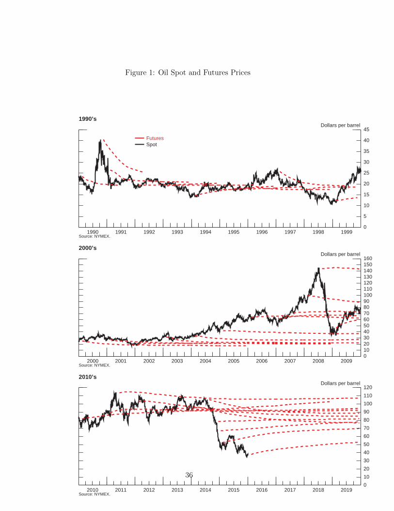
Figure 1: Oil Spot and Futures Prices

0

5

10

15

20

25

30

35

40

45

1990 1991 1992 1993 1994 1995 1996 1997 1998 1999

1990’sDollars per barrel

FuturesSpot

Source: NYMEX.

0 10 20 30 40 50 60 70 80 90 100 110 120

2010 2011 2012 2013 2014 2015 2016 2017 2018 2019

2010’sDollars per barrel

Source: NYMEX.

0 10 20 30 40 50 60 70 80 90 100 110 120 130 140 150 160

2000 2001 2002 2003 2004 2005 2006 2007 2008 2009

2000’sDollars per barrel

Source: NYMEX.

36

Figure 2: Estimates of Oil-Price Trend and Persistence of Transitory Shocks

2000 2005 2010 2015

−0.01

0

0.01

0.02

0.03

µ φ

2000 2005 2010 2015

0

0.2

0.4

0.6

0.8

1

1.2

1.4

37

Figure 3: Estimated Standard Deviations of Permanent and Transitory Shocks

σp

2000 2005 2010 20150

0.05

0.1

0.15

0.2

στ

2000 2005 2010 20150

0.05

0.1

0.15

0.2

38

Figure 4: The Relative Importance of Permanent Shocks

2000 2005 2010 20150

0.1

0.2

0.3

0.4

0.5

0.6

0.7

0.8

0.9

1

39

Figure 5: Predicting Futures Prices

2000 2005 2010 20150

20

40

60

80

100

120

140

160

180

Dol

lars

Per

Bar

rel

Spot Price2−year Ahead Futures Prices (Data)2−year Ahead Futures Prices (Model)

40

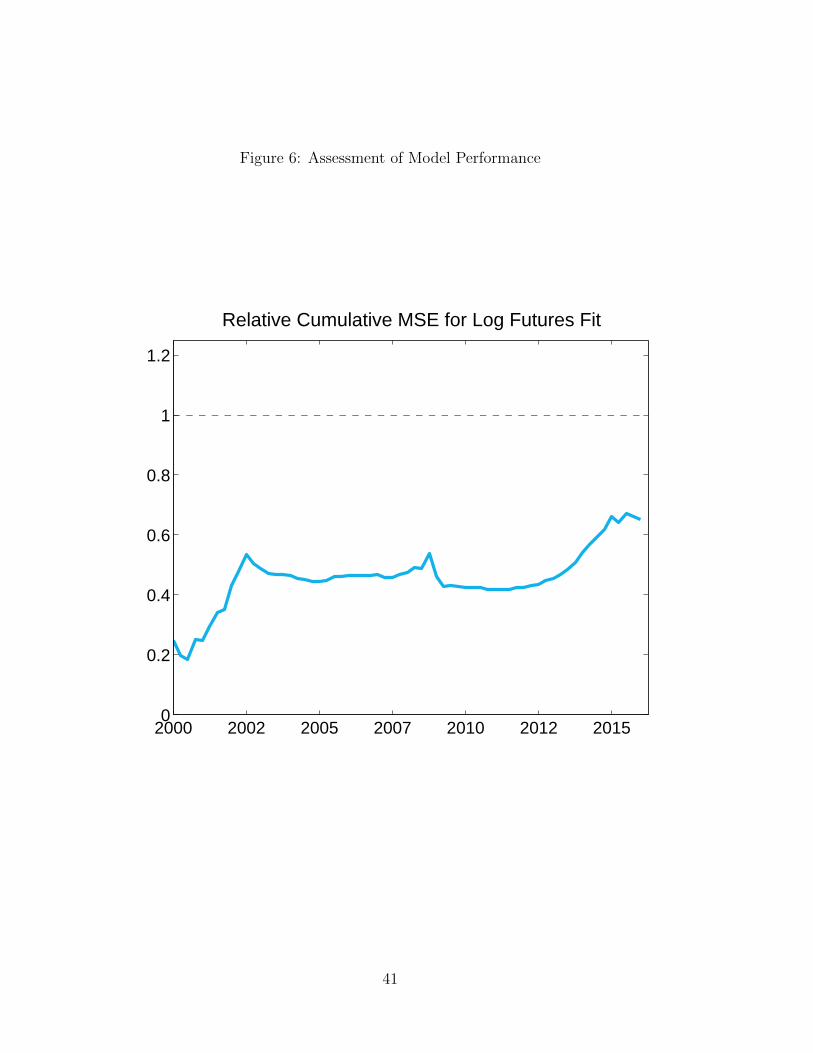
Figure 6: Assessment of Model Performance

Relative Cumulative MSE for Log Futures Fit

2000 2002 2005 2007 2010 2012 20150

0.2

0.4

0.6

0.8

1

1.2

41

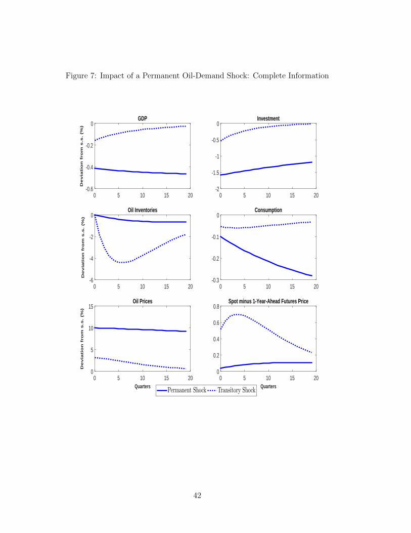
Figure 7: Impact of a Permanent Oil-Demand Shock: Complete Information

0 5 10 15 20

De

via

tio

n f

rom

s.s

. (%

)

-0.6

-0.4

-0.2

0GDP

0 5 10 15 20 -2

-1.5

-1

-0.5

0Investment

0 5 10 15 20

De

via

tio

n f

rom

s.s

. (%

)

-6

-4

-2

0Oil Inventories

0 5 10 15 20 -0.3

-0.2

-0.1

0Consumption

Quarters0 5 10 15 20

De

via

tio

n f

rom

s.s

. (%

)

0

5

10

15Oil Prices

Quarters0 5 10 15 20

0

0.2

0.4

0.6

0.8Spot minus 1-Year-Ahead Futures Price

Permanent Shock Transitory Shock

42

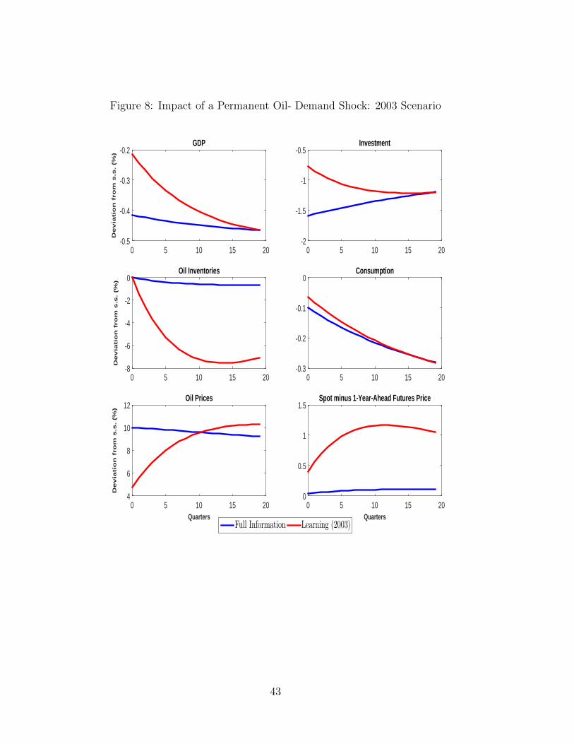
Figure 8: Impact of a Permanent Oil- Demand Shock: 2003 Scenario

0 5 10 15 20

De

via

tio

n f

rom

s.s

. (%

)

-0.5

-0.4

-0.3

-0.2GDP

0 5 10 15 20 -2

-1.5

-1

-0.5Investment

0 5 10 15 20

De

via

tio

n f

rom

s.s

. (%

)

-8

-6

-4

-2

0Oil Inventories

0 5 10 15 20 -0.3

-0.2

-0.1

0Consumption

Quarters0 5 10 15 20

De

via

tio

n f

rom

s.s

. (%

)

4

6

8

10

12Oil Prices

Quarters0 5 10 15 20

0

0.5

1

1.5Spot minus 1-Year-Ahead Futures Price

Full Information Learning (2003)

43

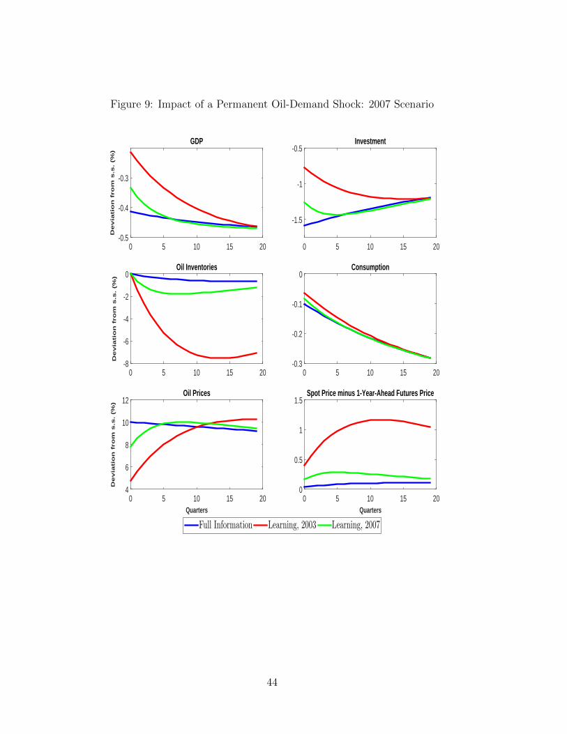
Figure 9: Impact of a Permanent Oil-Demand Shock: 2007 Scenario

0 5 10 15 20

De

via

tio

n f

rom

s.s

. (%

)

-0.5

-0.4

-0.3

GDP

0 5 10 15 20

-1.5

-1

-0.5Investment

0 5 10 15 20

De

via

tio

n f

rom

s.s

. (%

)

-8

-6

-4

-2

0Oil Inventories

Quarters0 5 10 15 20

De

via

tio

n f

rom

s.s

. (%

)

4

6

8

10

12Oil Prices

Quarters0 5 10 15 20

0

0.5

1

1.5Spot Price minus 1-Year-Ahead Futures Price

Full Information Learning, 2003 Learning, 2007

0 5 10 15 20 -0.3

-0.2

-0.1

0Consumption

44

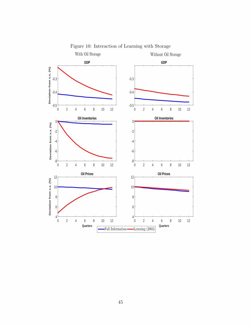
Figure 10: Interaction of Learning with Storage

0 2 4 6 8 10 12

De

via

tio

n f

rom

s.s

. (%

)

-0.5

-0.4

-0.3

GDP

0 2 4 6 8 10 12

De

via

tio

n f

rom

s.s

. (%

)

-8

-6

-4

-2

0Oil Inventories

Quarters0 2 4 6 8 10 12

De

via

tio

n f

rom

s.s

. (%

)

4

6

8

10

12Oil Prices

0 2 4 6 8 10 12 -0.5

-0.4

-0.3

GDP

0 2 4 6 8 10 12 -8

-6

-4

-2

0Oil Inventories

Quarters0 2 4 6 8 10 12

4

6

8

10

12

With Oil Storage Without Oil Storage

Oil Prices

Full Information Learning (2003)

45

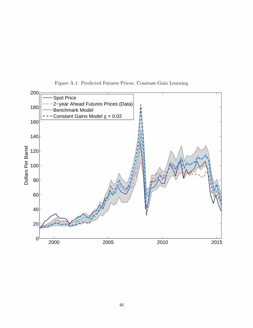
Figure A.1: Predicted Futures Prices: Constant-Gain Learning

Dol

lars

Per

Bar

rel

2000 2005 2010 20150

20

40

60

80

100

120

140

160

180

200Spot Price2−year Ahead Futures Prices (Data)Benchmark ModelConstant Gains Model χ = 0.02

46

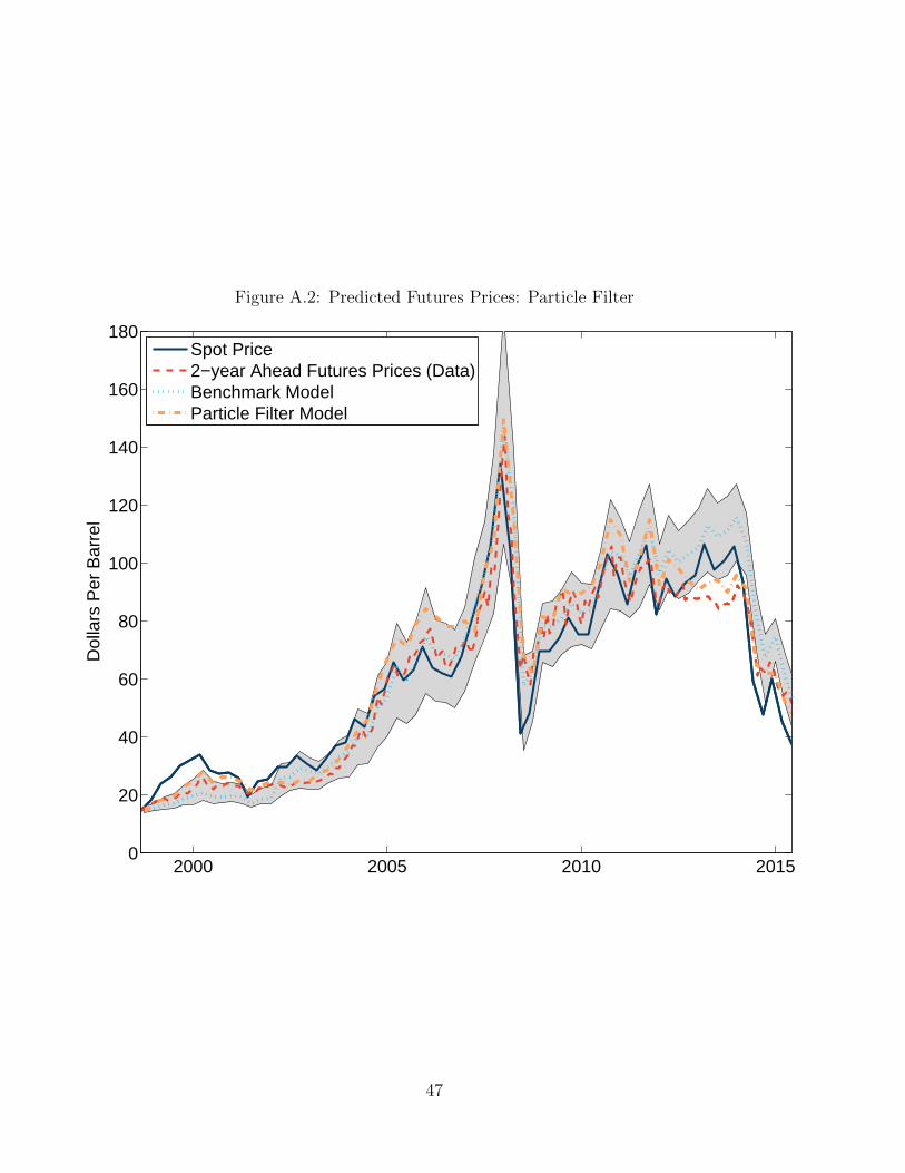
Figure A.2: Predicted Futures Prices: Particle Filter

2000 2005 2010 20150

20

40

60

80

100

120

140

160

180

Dol

lars

Per

Bar

rel

Spot Price2−year Ahead Futures Prices (Data)Benchmark ModelParticle Filter Model

47