M A X P L A N C K S O C I E T Y

Preprints of theMax Planck Institute for

Research on Collective GoodsBonn 2011/26

Learning in experimental 2 x 2 games

Thorsten Chmura Sebastian J. Goerg Reinhard Selten

Preprints of the Max Planck Institute for Research on Collective Goods Bonn 2011/26

Learning in experimental 2 x 2 games

Thorsten Chmura, Sebastian J. Goerg, Reinhard Selten

October 2011

Max Planck Institute for Research on Collective Goods, Kurt-Schumacher-Str. 10, D-53113 Bonn http://www.coll.mpg.de

Learning in experimental 2× 2 games

Thorsten Chmuraa, Sebastian J. Goergb,∗, Reinhard Seltenc

aDepartment of Economics, Ludwig-Maximilians-Universitat MunichbMax Planck Institute for Research on Collective Goods, Bonn

cLaboratory for Experimental Economics (BonnEconLab), University of Bonn

Abstract

In this paper, we introduce two new learning models: impulse-matching learning andaction-sampling learning. These two models together with the models of self-tuningEWA and reinforcement learning are applied to 12 different 2 × 2 games and theirresults are compared with the results from experimental data. We test whether themodels are capable of replicating the aggregate distribution of behavior, as well ascorrectly predicting individuals’ round-by-round behavior. Our results are two-fold:while the simulations with impulse-matching and action-sampling learning success-fully replicate the experimental data on the aggregate level, individual behavior isbest described by self-tuning EWA. Nevertheless, impulse-matching learning has thesecond highest score for the individual data. In addition, only self-tuning EWAand impulse-matching learning lead to better round-by-round predictions than theaggregate frequencies, which means they adjust their predictions correctly over time.

Keywords: Learning, 2× 2 games, Experimental data

JEL: C72, C91, C92

1. Introduction

It is well known that rational learning, in the sense of Bayesian updating, leadsto the stationary points of the Nash equilibrium (e.g., Kalai and Lehrer, 1993).But it also known that actual human behavior not necessarily converges to Nashequilibrium. In fact, a vast body of literature indicates situations in which standardtheory does not perform as a good predictor for subjects’ behavior in experiments(e.g., Brown & Rosenthal, 1990, Erev & Roth, 1998).

A recent publication by Selten & Chmura (2008) documents the predominanceof behavioral stationary concepts regarding descriptive power. In the paper, theconcepts of impulse-balance equilibrium (Selten & Chmura, 2008), payoff-samplingequilibrium (Osborne & Rubinstein, 1998), action-sampling equilibrium (Selten &Chmura, 2008) and quantal response equilibrium (McKelvey & Palfrey, 1995) out-perform Nash equilibrium in describing the decisions of a population in twelve

∗Corresponding author. Kurt-Schumacher-Str. 10, 53113 Bonn, Germany,Tel.: +49 228 91416 39; fax: +49 228 9141662.

Email address: goerg@coll.mpg.de (Sebastian J. Goerg)

1

completely mixed 2 × 2 games. Moreover, payoff-sampling equilibrium and action-sampling equilibrium perform better than quantal response equilibrium does. In ad-dition the parameter-free concept of impulse-balance equilibrium performs equallywell as the parametric concept of quantal response equilibrium.1 Furthermore, Go-erg & Selten (2009) show that the advantage of impulse-balance equilibrium overNash equilibrium is not limited to 2 × 2 games, but also present in cyclic duopolygames.

Presumably stationary behavior is a result of a learning process converging toa stationary distribution of actions for both players, which is, as the above studiesdemonstrate, not necessarily the Nash equilibrium. Therefore, constructing andtesting simple learning models with the predicted stationary states of the betterperforming concepts suggests itself. For the two behavioral stationary concepts ofaction-sampling equilibrium and impulse-balance equilibrium this is quite easy: bothyield precise expression for stationary behavior.

The main purpose of this article is to introduce two new learning models whichare based on the behavioral reasoning of action-sampling equilibrium and impulse-balance equilibrium and test them in the environment of twelve repeated 2×2 gameswith mixed equilibria. Hereby, the learning rules have to meet two challenges: first,do they reproduce the aggregate behavior of a human population, and second, canthey adequately describe the observed behavior of a single individual?

For comparison, we include the models of reinforcement learning (Erev & Roth,1995) and self-tuning experience-weighted attraction learning (Ho, Camerer & Chong,2007). We decided to compare our results with reinforcement learning, as it was thefirst model with application of rote learning to economics and it is the most citedlearning model in economics. Self-tuning EWA was selected to cover a broader setof different learning variants, as it can describe weighted fictitious play, averagingreinforcement learning, and models in between.2

For the analysis on the aggregate level, we conduct simulations with the fourlearning models and the twelve 2× 2 games experimentally investigated in Selten &Chmura (2008). The simulations replicate the exact situation of the experiments.In each simulation run, eight agents, four deciding as row players and four decidingas column players, are randomly matched in each round over 200 rounds. In eachsimulation run, one game is played and one learning model is applied. To judge thepredictive power on the aggregate level we compare the distribution of choices in thesimulation runs with the experimental data from Selten & Chmura (2008).

To investigate how well the learning models predict individuals’ behavior, we

1For further discussions please refer to Brunner, Camerer & Goeree (2011) and Selten, Chmura& Goerg (2011).

2We decided not to include a pure version of fictitious play in our analyses since a populationof fictitious players would converge in the 2 × 2 games to the Nash equilibrium (Miyasawa, 1961,and Metrick & Polak, 1994), which is clearly outperformed by the stationary concepts of impulse-balance equilibrium and action-sampling equilibrium (Selten & Chmura, 2008). However, withaction-sampling learning and self-tuning EWA variants of fictitious play are included into ouranalyzes. Furthermore, in this paper we solely focus on learning rules with at most one parameter.Thus, more elaborate versions of fictitious play with additional parameters like the three parametermodel by Cheung & Friedman (1997) and the six parameter model of Chen et al (2011) are ignored.

2

separately evaluate the explanatory power of the learning models for each participantof the 2×2 experiments. For each of the 864 subjects we compare the actual decisionin every round with the decision predicted by the learning model given the subject’shistory. To judge the power of the learning models, we introduce three benchmarkswhich all learning models should beat. The first benchmark is the inertia rule, whichpredicts for each round the same choice as executed in the round before. The secondbenchmark is a random play with equal probability for each of the two decisions.In addition, if the learning theories describe subjects’ behavior correctly over time,their predictions should be more accurate than the observed aggregate frequencies.Thus, as a more demanding benchmark, we include the empirical frequencies as acriterion.

As Erev, Ert, & Roth (2010) state, there are three obstacles for the learningliterature: 1. small data sets, 2. problems of over-fitting (Salmon, 2001; Hopkins,2002), and 3. relative small sets of models. We try to address these issues by1.) using the large data set of Selten & Chmura (2008) with twelve 2 × 2 gamesplayed by 864 subjects, 2.) using theories with at most one parameter , adjustingthe parameters over all games and applying only nonparametric analysis, and 3.)applying and testing four different learning models. In fact, the results presentedin this paper are the condensed summary of the analyses with 7 learning models.In addition to the already mentioned models, we introduce and test the conceptsof payoff-sampling learning and impulse-balance learning. Because both conceptsperform worse than the inertia benchmark and the random play benchmark, we donot cover these two learning models in more detail. More information about thesetwo models can be found in the Appendix. To shed some additional light on theperformance of self-tuning EWA, we include a non-parametric version of self-tuningEWA into our analyzes. We will refer to these results in the discussion. Additionalinformation about the omitted concepts as well as the comparison of all 7 learningmodels can be found in the appendix.

Our results are twofold: our newly introduced models are able to capture the dis-tribution of decisions on the aggregate level much better than self-tuning EWA andreinforcement does, while self-tuning EWA describes the individual data in a muchmore accurate way. On the aggregate level the learning models of impulse-matchinglearning and action-sampling learning have the smallest distance to the experimen-tal data, while the concepts of self-tuning EWA and reinforcement learning haverelatively high distances to the data. On the individual level, self-tuning EWA andimpulse-matching have the highest scores. In addition, these two learning conceptsare the only concepts that perform significantly better in describing individual roundby round behavior then the overall empirical frequencies.

2. The Learning Models

In the following, we will introduce impulse-matching learning and action-samplinglearning, which are based on the behavioral stationary concepts discussed in Selten& Chmura (2008). In addition to the new learning models, the more establishedconcepts of reinforcement learning (c.p. Erev & Roth, 1998) and self-tuning EWA(Ho, Camerer & Chong , 2007) are briefly explained.

3

Two of the discussed models, namely action-sampling learning and self-tuningEWA are parametric concepts. In case of action sample learning the parameteris the sample size. Self-tuning EWA is based on the multi-parametric concept ofexperience-weighted attraction learning (Camerer & Ho, 1999). Self-tuning EWAreplaces two of the parameters with numerical values and two with functions. The re-maining parameter λ ”measures sensitivity of players to attractions” (p. 835 Camerer& Ho, 1999). The version of reinforcement learning examined here does not have aparameter and the initial propensities are not estimated from the data. All inves-tigated learning rules will start with randomization of .5 in the first round. Onlyafter all necessary information has been gathered, the corresponding learning ruledetermines the following decisions.3

The parameters of the parametric concepts are estimated to lead to the best fitover all data and over all games. For more details about the parameter estimationon the aggregate level, refer to the results section 4.2; for details on the estimationof the parameters on the individual level, refer to results section 5.2.

2.1. Impulse Matching Learning

Impulse-matching learning relates to the concepts of impulse-balance equilibrium(Selten, Abbink & Cox, 2005 and Selten & Chmura, 2008) and learning directiontheory (Selten & Stoecker, 1986 and Selten & Buchta, 1999). After a decision andafter the realization of the payoffs, the behavior is adjusted to experience. Seltenand Buchta explain the concept by the example of a marksman aiming at a trunk:”If he misses the trunk to the right, he will shift the position of the bow to the left andif he misses the trunk to the left he will shift the position of the bow to the right. Themarksman looks at his experience from the last trial and adjusts his behavior [...].”(p. 86 Selten & Buchta, 1999). Impulse-balance equilibrium and impulse-matchinglearning overcome the limitation of learning direction theory defining a directiononly for ordered strategies, e.g., increasing a bid in an auction (cf. Ho, Camerer &Chong , 2007) by shifting the probabilities of single actions.

To understand how impulse-matching learning works, suppose that in a periodthe first of two actions has been chosen and that this action was not the best reply tothe action played by the other player. Then the player receives an impulse towardsthe second action. Originally, an impulse was defined as the difference between thepayoff the player could have received for his best reply minus the payoff actuallyreceived given the decision by the other player in this period. However, the theoryof impulse-matching learning is based on another impulse concept. Here, a playeralways receives an impulse from the action with the lower payoff to the one with thehigher payoff. The resulting learning model is similar to the regret-based learningmodels, which have already been successfully tested by Marchiori & Warglien (2008).The name impulse-matching is due to the fact that this kind of learning leads toprobability matching by a player if the probabilities p1 and (1 − p1) on the otherside are fixed, and the payoffs for the player is one if both players play the strategy

3This means, for example, that for impulse-matching learning, impulses into both directionsmust have been experienced by the subject, and for reinforcement learning payoff-sums for bothactions must have been collected.

4

with the same number (one or two) and zero otherwise (cf. Estes, 1954).To incorporate loss aversion, the impulses are not calculated with the original

payoffs, but with transformed ones. In games with two pure strategies and a mixedNash equilibrium, each pure strategy has a minimal payoff and the maximum ofthe two minimal payoffs is called the pure strategy maximin. This pure strategymaximin is the maximal payoff a player can obtain for sure in every round and itforms a natural aspiration level. Amounts below this aspiration level are perceivedas losses and amounts above this aspiration level are perceived as gains. In linewith prospect theory (Kahneman & Tversky, 1979), losses are counted double incomparison to gains. Thus, gains (the part above the aspiration level) are cut tohalf for the computation of impulses. Figure 1 is taken from Selten & Chmura (2008)and illustrates the transformation of the payoffs by the example of game 3.

3

Figure 2: The curves for pU and qL arising in the example of game 1 for each of the five

concepts.

Figure 3: Impulse Balance Transformation for the example of experimental game 3.

Figure 4: Impulse in the direction of the strategy not chosen.

Figure 1: Example of matrix transformation as given in Selten & Chmura (2008)

Impulse-matching learning can be described as a process in which a subject formsimpulse sums. The impulse sum Ri(t) is the sum of all impulses from j towards iexperienced up to period t−1. The probabilities for playing action 1 and 2 in periodt are proportional to the impulse sums R1(t) and R2(t) :

pi(t) =Ri(t)

R1(t) +R2(t), for i = 1, 2 (1)

The impulses from action j towards action i in period t are as follows:

ri(t) = max[0, πi − πj] (2)

for i, j = 1, 2 and i 6= j. Here, πi is the transformed payoff for action i given thematched agents decision and πj the one for action j. Afterwards the impulse sumsare updated with the new impulses:

Ri(t+ 1) = Ri(t) + ri(t) (3)

In the first round, all impulse sums are zero R1(1) = R2(1) = 0, and until bothimpulse sums are higher than zero, the probabilities are fixed to p1(t) = p2(t) = 0.5.

5

2.2. Action Sampling Learning

Action-sampling learning relates to the idea of the action-sampling equilibriumof Selten & Chmura (2008). According to action-sampling equilibrium, a playertakes in the stationary state a fixed size sample of the pure strategies played by theother players in the past and optimizes against this sample. The process of action-sampling learning is a belief-based type of learning, which is very similar to fictitiousplay. In fact, the model by Chen et al (2011) is a generalization of action-samplinglearning, which captures in addition inertia, recency and weighting of the grandmean. Action-sampling learning is much simpler and can be described as a versionof fictitious play where only random periods are considered and not the whole datafrom the history.

In the process of action-sampling learning, the agent randomly takes a sampleA(t) with replacement of n earlier actions a1, ..., an of the other player. Let πi(aj)be the payoff of action i if the opponent plays action aj. For i = 1, 2 let Pi(t) =∑n

j=1 πi(aj) be the sum of all payoffs of the player for using her action i against theactions in this sample.

Therefore, in period t, the player chooses her action according to

pi(t) =

1 if Pi(t) > Pj(t)

0.5 if Pi(t) = Pj(t)

0 else

(4)

for i, j = 1, 2 and i 6= j.At the beginning, the probabilities are set to p1 = p2 = 0.5, until both possible

actions have been played by the opponent agents.

2.3. Reinforcement Learning

The concept of reinforcement learning is one of the oldest and best establishedlearning models in the literature; refer to Harley (1981) for an early application. Forexperimental economics, it was first formulated and introduced by I. Erev and A.E. Roth ( Erev & Roth,1995, and Roth & Erev, 1998). In the reinforcement model,a player builds up a payoff sum Bi(t) for each action i according to the followingformula:

Bi(t+ 1) =

{Bi(t) + π(t) if action i was chosen in t

Bi(t) else.(5)

Here π(t) is the payoff obtained in period t. After an initial phase in which bothpossible actions are used with equal probabilities, the probability of choosing actioni in period t is given by:

pi(t) =Bi(t)

B1(t) +B2(t)(6)

This model presupposes that all payoffs in a player’s payoff matrix are non-negative and at least one payoff in each column and row is positive, a condition

6

fulfilled by all twelve investigated games.4 In the first round, the initial payoff sumsBi(t) are zero and the player chooses both possible actions with equal probabilitiesp1 = p2 = .5. The initial phase ends as soon as both sums are positive, and onlyfrom then on, equation 6 is applied to determine the probabilities.

Impulse matching learning and action-sampling learning are both based on be-havioral stationary concepts. Reinformcent learning can converge to Nash equilib-rium (Beggs, 2005) and therefore, we treat it in the following as the learning conceptthat corresponds with Nash equilibrium.

2.4. Self-Tuning EWA

Self-tuning EWA was introduced by Ho, Camerer, & Chong (2007). It is basedon the experience-weighted attraction model (Camerer & Ho, 1999), but replacesall but one parameter of this model with functions or fixed values. Of all modelsdiscussed in this article, self-tuning EWA is the most sophisticated one because it cancapture different types of learning. The decisions are made according to attractionsAi(t) for each strategy i. Attractions are based on the payoffs π(si, s

m(t)) which asubject would have received for playing strategy si given the actual decision sm(t)by the matched player. The attraction updating function depends on an experienceweight N(t), a change-detector function φ(t), and the attention function δ(t):

Ai(t) =φ(t)N(t− 1)Ai(t− 1) + [δ(t) + (1− δ(t))I(si, s(t))]π(si, s

m(t))

N(t)(7)

Here I(x, y) is an indicator function equal to 1 for s(t) = si and 0 otherwise. Anexperience weight is applied to each attraction and it is defined as

N(t) = N(t− 1)φ(t) + 1, with N(0) = 1. (8)

The change-detector function φ(t) weights lagged attractions and represents ”a player’sperception of how quickly the learning environment is changing”(p. 182, Ho, Camerer,& Chong, 2007). It is defined as

φ(t) = 1− 1

2S(t) (9)

with S(t) being the so called surprise index, which measures the deviation of thematched players’ recent decisions from all previous decisions.5 S(t) is the quadraticdistance between the cumulative history vector hmk (t) and the immediate historyvector rmk (t) for the k strategies of the matched player m. The cumulative historyvector gives the relative frequency over all rounds and is defined as

hmk (t) =

∑tτ=1 I(smk , s

m(τ))

t. (10)

4For games with negative payoffs, this approach would not be adequate. To cope with negativepayoffs, the model used by Erev & Roth (1998) replaces the payoff π(t) in E.1 by π(t) − πmin,where πmin is the smallest possible payoff of the player.

5The experiments were played with random matching and thus no identification of single playersis possible. Therefore, we assume that all matched players are perceived as one average player.

7

The immediate history vector gives the relative frequency in the recent rounds. For2× 2 games with mixed equilibria, it is defined as

rmk (t) =2∑

k=1

(∑tτ=t−W+1 I(smk , s

m(τ))

W

), (11)

with W = 2. The surprise index is zero, if the strategy of the matched player didnot change from period t− 1 to t. Otherwise it is 1 and the matched player changesa lot between strategies.

S(t) =2∑

k=1

(hmk (t)− rmk (t))2 (12)

The attention function δ(t) generates a weight for foregone payoffs and turns theattention to strategies which would have yielded higher payoffs. In games with aunique mixed-strategy equilibrium, these payoffs are weighted with 1/W , with Wbeing the numbers of strategies played in equilibrium. Thus, in our 2×2 games withmixed equilibria, it is set to be W = 2.

δ(t) =

{1W

if π(sj, sm(t)) ≥ π(t)

0 else.(13)

The attention function δ(t) of self-tuning EWA captures the idea of learningdirection theory (Selten & Stoecker, 1986) that subjects have a tendency to moveinto the direction of the strategy which was ex-post the best response. This is doneby shifting the attention and thus the probability towards the strategy with thehighest payoff. This is similar to the process of impulse-matching learning. Theresulting probability of playing action i in period t, depending on the attractions, iscalculated as a logit response function:

pi(t) =eλAi(t−1)∑2j=1 e

λAj(t−1)(14)

Here, λ is the response sensitivity and this parameter must be specified to fitthe empirical data. To be consistent with the other models, we have chosen not toestimate any additional values and the simulations start with pure randomizationwith p1 = p2 = 0.5.

3. Games and Experiments

Our comparison of the investigated learning rules is based on the data of Selten& Chmura (2008). In their study, twelve 2× 2 games with pure equilibria in mixedstrategies were experimentally investigated. To cover a broad set of games, sixconstant and six non-constant sum games were played. Figure 2 shows the twelvegames used in the experiment. The constant sum games are shown on the left sideof the figure and the non-constant sum games on the right side.

Note that the first six games have the same best-response structure as the secondsix games and that the concepts of action-sampling equilibrium and Nash equilibrium

8

Constant sum games Non-constant sum gamesL R L R

Game 1U

10 0

Game 7U

10 48 18 12 22

D9 10

D9 14

9 8 9 8

L R L R

Game 2U

9 0

Game 8U

9 34 13 7 16

D6 8

D6 11

7 5 7 5

L R L R

Game 3U

8 0

Game 9U

8 36 14 9 17

D7 10

D7 13

7 4 7 4

L R L R

Game 4U

7 0

Game 10U

7 24 11 6 13

D5 9

D5 11

6 2 6 2

L R L R

Game 5U

7 0

Game 11U

7 22 9 4 11

D4 8

D4 10

5 1 5 1

L R L R

Game 6U

7 1

Game 12U

7 31 7 3 9

D3 8

D3 10

5 0 5 0

The payoffs for the column players are shown in the lower right corner,the payoff for the row palyers are shown in the upper left corner.

Abbreviations used: L Left, R Right, U Up, D Down

Figure 2: The twelve 2× 2-games taken from Selten & Chmura (2008).

only depend on this best response structure. Thus, the predictions of Nash equilib-rium are the same for the first and the second six games and the same holds true foraction-sampling equilibrium. The predictions of Nash equilibrium, action-samplingequilibrium and impulse-balance equilibrium are given in table 1.

All experiments were run at the BonnEconLab with students mainly majoringin economics or law. The experiment was programmed with RatImage developed byAbbink and Sadrieh (1995). The data was collected in 54 sessions with 16 subjectseach. In every session, only one game was played and this game was known by allsubjects. The games were played for 200 periods with matching groups consistingout of eight subjects. For each constant sum game twelve independent matchinggroups were gathered, for each non-constant sum game six independent matchinggroups were gathered. Overall, 864 subjects participated.

The role of the subjects was fixed for the whole experiment, thus four subjectsin each matching group decided as column players and the other four as row playersthroughout the whole experiment. At the beginning of each round, row and col-umn players were randomly matched. After every round, subjects received feedbackabout the other player’s decision, their own payoff, the period number and their

9

own cumulative payoff. Each participant received e 5 for showing-up. In addition,the payoffs in the 200 periods were accumulated and transferred into EURO. Theexchange rate was e 0.016 Cent per payoff point. An experimental session lastedbetween 1.5 and 2 hours and the average earning per subject was roughly e 24,including show-up fee.

4. Performance on the Aggregate Level

In this section, we investigate whether the learning algorithms can replicate theaggregate distribution of actions generated by human subjects. In the following, wewill first introduce our measurement for the aggregate level. Thereafter, we discussthe success of the different learning models in predicting/reproducing the aggregatedistribution of behavior.

4.1. Measure of Predictive Success on the Aggregate Level

For our analysis on the aggregate level, we conduct simulations keeping every-thing the same as in the experiment, except that instead of real participants nowcomputer agents interact. Each agent interacts according to her history and to thesame learning model over 200 rounds. In each round, eight agents with fixed roles,four deciding as row players and four as column players, are randomly matched andall agents act in accordance to the same learning rule.

After each round, they receive feedback about the matched agent’s decision andtheir payoff. Since none of the learning models makes use of the round number andsince the calculation of the cumulated payoff can be done by the agents themselves,this information is not provided to the agents. It is crucial that the agents do notreceive more information than the subjects in the experiment did.

All learning models include stochastic elements. To avoid the influence of sta-tistical outliers, 500 simulation runs per game are conducted. In each simulationrun, all agents act in accordance with the same learning model. To measure thepredictive success on the aggregate basis, we will compare the mean frequencies ofU and L in the simulations with the mean frequencies obtained in the experimentsby means of the quadratic distance. The mean quadratic distance Q is the averagequadratic distance over all 12 games and over all 500 simulations. It is defined as

Q =1

12

12∑i=1

(1

500

500∑n=1

(sLin − fLi )2 + (sUin − fUi )2

),

with sLin and sUin being the frequencies for L and U in game i and simulationrun n. Respectively, fLi and fUi are the mean frequencies for L and U observedin the experiments with game number i. The frequencies of R and D need not beconsidered in view of (sLin − fLi )2 = (sRin − fRi )2 and (sUin − fUi )2 = (sDin − fDi )2. Thepredictive success of a learning model increases with a decreasing mean quadraticdistance, i.e., the smaller the mean quadratic distance is, the better the learningtheory fits the experimental data on the aggregate level.

10

4.2. Parameter Estimates

The concepts of action-sampling equilibrium and self-tuning EWA have a param-eter which needs to be adjusted to the experimental data. We decided to estimatefor each learning model one parameter that minimizes the quadratic distance overall games.6 To estimate the optimal parameter, we ran for each parameter 500simulations per game and calculated the mean quadratic distance. Thereafter, thesimulations were conducted with the parameter that yielded the smallest quadraticdistance.7

0.0

2.0

4.0

6.0

8.1

Mea

n Q

uadr

atic

Dis

tanc

e

1 2 3 4 5 6 7 8 9 10 11 12 13 14 15Sample sizes

Action−sampling

0.0

2.0

4.0

6.0

8.1

Mea

n Q

uadr

atic

Dis

tanc

e

1 2 3 4 5 6 7 8 9 10 11 12 13 14 15Sample sizes

Payoff−sampling

Figure 3: Quadratic distances of action-sampling learning

The parameter of action-sampling learning is the size of the drawn samples.Figure 3 gives the mean quadratic distances of action-sampling learning for 1 ≥ n ≥15. A sample size of n = 12 leads to the smallest quadratic distance, which is thesame sample size that also leads to the smallest distance for the stationary concept(cf. Brunner, Camerer & Goeree, 2011)

Figure 4 gives the mean quadratic distances of self-tuning EWA for differentlambdas. The left part gives the mean quadratic distances for all tested lambdasbetween 0 and 10, and the right part gives the quadratic distance for .2 < λ < .3.

6One could fit the parameter of the parametric concepts for each game separately. We believethat this gives an unfair advantage to one-parameter theories over parameter-free ones. Thisespecially holds for the case of 2 × 2 games, where only two relative frequencies are predicted.Adjusting a parameter separately for each game, so to speak, does half the job. One might usemethods to adjust the fit of a theory to the number of parameters used, but this only makes senseif the non-adjusted performance of a model increased in case of parameters being estimated foreach game separately. For our simulations, only the quadratic distance of action-sampling learningwould benefit from such a procedure. The quadratic distance of self-tuning EWA (0.0805 vs.0.0786) would change only slightly and this adjustment would not influence the relative ranking ofquadratic distances. Therefore, we decided to estimate only one parameter for each theory.

7To speed up this procedure, round-by-round data was only saved for the simulations with thefinal parameter.

11

.1.2

.3.4

.5.6

Mea

n Q

uadr

atic

Dis

tanc

e

0 2 4 6 8 10Lambda

.080

5.0

81.0

815

.082

.082

5M

ean

Qua

drat

ic D

ista

nce

.2 .22 .24 .26 .28 .3Lambda

Figure 4: Quadratic distances of self-tuning EWA for different lambdas. Eachpoint represents the mean quadratic distance over 500 simulations per game. Leftfigure for 0 ≤ λ ≤ 10 and right figure for .2 ≤ λ ≤ .3

Each point in the graph represents the mean quadratic distance over all twelvegames with 500 simulations runs per game with one specific lambda value. Thevalue leading to the smallest quadratic distance is λ = 0.2775.

4.3. Relative Frequencies

Table 1 gives the observed mean frequencies for each learning type, mean fre-quencies predicted by the stationary concepts and the observed frequencies in theexperiments. For the experimental games 1 to 6, the mean frequencies observed in agame are based on the observed frequencies in twelve independent matching groups;for games 7 to 12 they are based on the observed frequencies in six independentmatching groups. Each matching group consists of eight subjects. For each learningtype and game, the mean is based on 500 simulation runs, which produced 500 inde-pendent matching groups per game. Each matching group consists of eight agents.Figure 5 gives the typical development of probabilities over time in game 7 for eachof the learning types. This figure in combination with Table 1 already reveals somedifferences between the learning rules.8

It is surprising that self-tuning EWA yields relative frequencies very near to .5for each of the twelve games. This is probably connected to the fact that, in oursimulations, the whole population is of the same type and agents try to adjust toan inaccurate history, and by this process generate a new inaccurate history forthemselves and the matched agents. Estimating the free parameter of this modeljointly for all games is not a reason for this behavior. If we estimate the optimal λfor each game separately, the resulting mean quadratic distance to the data improvesonly marginally (0.081 vs. 0.079) and observed relative frequencies do not change

8The course of probabilities for all games is given in Appendix in section Appendix C.1

12

Table 1: Relative frequencies for playing Let and Up in the simulations, predicted bythe stationary concepts and observed in the experiments for Up and Left

Impuls

e-m

atc

hin

gle

arnin

g

Act

ion-s

am

pling

learn

ing

Rei

nfo

rcem

ent

learn

ing

self

-tunin

gE

WA

lear

nin

g

Impuls

e-b

alance

equilib

rium

Act

ion-s

am

pling

equilib

rium

Nas

heq

uilib

rium

Sel

ten

&C

hm

ura

data

Game 1 L 0.574 0.710 0.345 0.499 0.580 0.705 0.909 0.690U 0.063 0.095 0.121 0.499 0.068 0.090 0.091 0.079

Game 2 L 0.495 0.571 0.333 0.477 0.491 0.584 0.727 0.527U 0.169 0.193 0.161 0.502 0.172 0.193 0.182 0.217

Game 3 L 0.770 0.763 0.503 0.541 0.765 0.774 0.909 0.793U 0.157 0.211 0.128 0.492 0.161 0.208 0.273 0.163

Game 4 L 0.714 0.711 0.587 0.548 0.710 0.719 0.818 0.736U 0.259 0.295 0.190 0.494 0.259 0.302 0.364 0.286

Game 5 L 0.632 0.639 0.566 0.524 0.628 0.643 0.727 0.664U 0.296 0.323 0.241 0.495 0.297 0.329 0.364 0.327

Game 6 L 0.602 0.596 0.666 0.527 0.600 0.596 0.636 0.596U 0.400 0.422 0.265 0.497 0.400 0.426 0.455 0.445

Game 7 L 0.637 0.709 0.380 0.564 0.634 0.705 0.909 0.564U 0.098 0.094 0.170 0.485 0.104 0.090 0.091 0.141

Game 8 L 0.563 0.572 0.396 0.540 0.561 0.584 0.727 0.586U 0.258 0.193 0.217 0.494 0.258 0.193 0.182 0.250

Game 9 L 0.767 0.762 0.525 0.600 0.764 0.774 0.909 0.827U 0.185 0.212 0.165 0.489 0.188 0.208 0.273 0.254

Game 10 L 0.726 0.711 0.640 0.587 0.724 0.719 0.818 0.699U 0.303 0.295 0.219 0.487 0.304 0.302 0.364 0.366

Game 11 L 0.648 0.640 0.609 0.572 0.646 0.643 0.727 0.652U 0.354 0.324 0.289 0.492 0.354 0.329 0.364 0.331

Game 12 L 0.605 0.596 0.560 0.578 0.604 0.596 0.636 0.604U 0.466 0.422 0.342 0.494 0.604 0.426 0.455 0.439

much.Impulse-matching learning and action-sampling learning are quite close to their

stationary counterparts after 200 periods. The quadratic distances between impulse-

13

0.2

.4.6

.8

0 50 100 150 200Round

Impulse matching

0.2

.4.6

.8

0 50 100 150 200Round

Action sampling0

.2.4

.6.8

0 50 100 150 200Round

Reinforcement

0.2

.4.6

.8

0 50 100 150 200Round

self−tuning EWA

0.2

.4.6

.8

0 50 100 150 200Round

Experiment

Figure 5: Mean probabilities for left and right in the simulations runs and theexperiment for game 7 . Mean probability for left is given in black and the meanprobability for up is given in gray.

matching learning and impulse-balance equilibrium, as well as the one betweenaction-sampling learning and action-sampling equilibrium, are smaller than 0.001.If we treat reinforcement learning as the learning counterpart to Nash equilibrium,the difference in quadratic distances is 0.158. Self-tuning EWA has the highest dis-tances towards all stationary concepts. This closeness results in high correlationsbetween the frequencies of the simulations and corresponding stationary concepts.For impulse-matching learning and action-sampling learning, this is true for bothplayers (pairwise correlation with r > .9 and p < .01 for row and column players),and for reinforcement only for row players (pairwise correlation with r > .9 andp < .01). Correlations between observed frequencies from the experiments and thesimulations with action-sampling learning and impulse-matching learning are high(pairwise correlation with r > .8 and p < .01 for both playes), but lower than theones with the stationary concepts. The frequencies of reinforcement learning arecorrelated with the ones of the row player in the experiment (pairwise correlationwith r > .8 and p < .01), but not for the ones of the column players. The frequenciesof self-tuning EWA are not significantly correlated with the empirical data for eachof both players.

14

0.0

2.0

4.0

6.0

8

Reinfor

cemen

t

self−

tuning

EWANas

h

Impu

lse Bala

nce

Action S

amplin

g

Action S

amplin

g

Impu

lse M

atchin

g

Figure 6: Mean quadratic distances of the stationary concepts and the learningmodels to the observed behavior (stationary concepts dark bars and learning modelsin light bars).

4.4. Overall Performance

Figure 6 gives the mean of the quadratic distance between the experiment andsimulations over all games and rounds for self-tuning EWA learning, reinforcementlearning, action-sample learning and impulse-matching learning. In addition, thefigure gives the mean quadratic distances between of the stationary counterparts (ifexisting) and the data in black.9

We first turn our attention to the comparison of the simulations. The figurereveals a clear order of explanatory power. The order from worst to best (highestquadratic distance to lowest quadratic distance) is as follows: reinforcement learning,self-tuning EWA learning, action-sampling learning and impulse-matching learning.Because of the high number of observations (6000 per learning type), the order givenby Figure 6 is statistically robust (for all p < 0.01 Fisher-Pitman permutation test forpaired replicates). The difference between self-tuning EWA and reinforcement is verysmall and irrelevant. However, the similarity between the two quadratic distancesdoes not mean that both theories make similar predictions. This can be seen forexample in Table 1 and in Figure 5. The figure demonstrates that the concepts ofself-tuning EWA and reinforcement fail to describe the aggregate behavior in the2 × 2 experiments, in contrast to the other concepts. The quadratic distance ofself-tuning EWA is 18 times higher than the one of impulse-matching learning.

9The mean quadratic distances of the stationary concepts are either taken from Selten & Chmura(2008) or from Brunner, Camerer, & Goeree (2011). There were some flaws in the paper by Selten& Chmura (2008). For a detailed discussion, refer to Brunner, Camerer, & Goeree (2011) andSelten, Chmura, & Goerg (2011).

15

The quadratic distances of reinforcement learning and self-tuning EWA learningare significantly bigger not only over all games, but also for the subsets of constantsum games and non-constant sum games. However, reinforcement performs betterin constant sum games than self-tuning EWA does, while self-tuning EWA performsbetter in non-constant sum games (both p < 0.01 Fisher-Pitman permutation testfor paired replicates). While the quadratic distance of impulse-matching is stable inconstant and non-constant sum games, the one of action-sampling learning is smallerin constant sum games. Thus, action-sampling learning performs significantly betterin constant sum games, and impulse-matching learning performs significantly betterin non-constant sum games (both p < 0.01 Fisher-Pitman permutation test forpaired replicates).10

Comparing the stationary concepts with the learning models reveals that self-tuning EWA and reinforcement learning are not only outperformed by impulse-matching learning and action-sampling learning, but by all stationary concepts. Incontrast, the learning models of action-sampling and impulse-matching perform verywell. Both learning models have higher predictive success than the other learningmodels and additionally a higher predictive success than all stationary concepts.

4.5. Original Versus Transformed Games

The concept of impulse-matching learning is applied to the transformed gamerather than the original one. This transformation is an essential part of impulse-matching learning and impulse-balance equilibrium (Selten & Chmura, 2008; andGoerg & Selten, 2009), because both concepts involve a fixed loss-aversion. Losseswith respect to the pure strategy maximin are counted double. While double count-ing of losses with respect to the pure-strategy maximin is an essential part of impulse-matching learning, it is ignored by the other concepts (reinforcement learning, action-sampling learning, self-tuning EWA). This raises the question, whether the goodperformance of impulse-matching learning is an artifact of the incorporation of loss-aversion. To investigate this point, we apply all learning models to the transformedand to the original matrices.

Figure 7 shows the overall mean quadratic distances for self-tuning EWA learning,reinforcement learning, payoff-sampling learning, impulse-balance learning, action-sampling learning and impulse-matching learning applied to the original games andto the transformed games, which are again based on 500 simulation runs per gameand learning model.

It can be seen that impulse-matching learning and reinforcement learning per-form better when applied to the transformed games, whereas self-tuning EWA learn-ing and action-sampling learning do less well. While the improvement of impulse-matching learning in transformed games is expected, the benefit of applying rein-forcement learning to transformed games is unexpected. This improvement is sub-stantial, in the original game the quadratic distance is nearly 1.3 times higher thanin the transformed ones.

10Refer to the Appendix for more information about the performance in constant and non-constant sum games.

16

0.0

2.0

4.0

6.0

8M

ean

quad

ratic

dis

tanc

e

Reinforcement self-tuning EWA Action Sampling Impulse Matching

origin

al

trans

formed

origin

al

trans

formed

origin

al

trans

formed

origin

al

trans

formed

Figure 7: Mean quadratic distance in original and transformed games

0.0

2.0

4.0

6.0

8.1

Mea

n qu

adra

tic d

ista

nce

Reinforcement self-tuning EWA Action Sampling Impulse Matching

1-100

101-2

001-1

00

101-2

001-1

00

101-2

001-1

00

101-2

00

Figure 8: Mean quadratic distance over time

The theory of Roth and Erev (1998) applies a transformation of the original gameby replacing the payoff of a player by its difference to the minimal value in her matrix.The transformation used here is different since it involves double weights for losseswith respect to the pure strategy maximin. However, in Selten & Chmura (2008),no improvement of the predictive power of the Nash equilibrium was observed whenapplied to the transformed game rather than to the original one. It is interesting that

17

the picture looks different for the simulations over 200 rounds with reinforcementlearning, although it corresponds very much with Nash equilibrium (Beggs, 2005).

Although reinforcement learning improves when applied to the transformed ma-trix, it still performs significantly worse than impulse-matching learning. Therefore,and because of self-tuning EWA and action-sampling learning performing worse inthe transformed matrices, we can conclude that the good performance of impulse-matching learning is not driven by the transition to the transformed matrices alone.

4.6. Changes over Time

Learning processes are always dependent on time and history, and therefore itis of interest to check whether our above results remain stable over time. To checkstability of the order of explanatory power over time, we compare the first hundredperiods with the second hundred periods. Figure 8 gives the mean quadratic dis-tances for periods 1-100 (left) and 101-200 (right) for the six learning models. Thebasis of the comparison is always the observed mean frequencies for the correspond-ing rounds (either round 1-100 or 101-200) in the experiments.

It is easy to recognize, that in the second half of the simulation runs, the explana-tory power of self-tuning EWA and reinforcement learning decreases significantlywhile the one of impulse-matching learning improves significantly (all Fisher-Pitmanpermutation test for paired replicates p < 0.01). The concept of action-samplinglearning is rather stable over time and the statistically significant disimprovementof action-sampling learning (p < 0.01) is economically negligible, with an increaseof the quadratic distances of only 0.0004.

The ranking of concepts by mean quadratic distances is stable over time, theoverall ranking for round 1-200 is the same in rounds 1-100 and 101-200.

5. Performance on the Individual Level

In this part, we investigate how well the learning rules describe the individualbehavior of the subjects in the 2 × 2 experiments. To judge the performance onthe individual level, we compare the individual decisions in every round with thepredicted decisions or predicted probability by the learning rule, given the historyof the subject.

5.1. Measure of Predictive Success on the Individual Level

To measure the predictive success of the learning theories describing the behaviorof a single individual, we apply the quadratic scoring rule on each of the 864 subjectsfor each learning rule.11 The quadratic scoring rule was first introduced by Brier(1950) in the context of weather forecasting. The rationale behind the quadraticscoring rule is that for each round a score is determined, which evaluates the nearnessof the predicted probability distribution to the observed outcome.

11Of course, one could calculate the proportions of subjects that are described best by eachlearning rule. But this calculation of proportion is problematic: it depends on the number andthe performance of included learning concepts. Given that the score of one learning rule does notdepend on the competing learning concepts, we prefer to use the mean quadratic scores.

18

In Selten (1998), the quadratic scoring rule is axiomatically characterized. Thecharacterizing properties of the quadratic scoring rule, as described in Selten (1998),are: symmetry, elongational invariance, incentive compatibility, and neutrality. Sym-metry means that the score of a theory must not depend on the numbering of thedecision alternatives. Elongational invariance assures that the score of a theory isnot influenced by adding or leaving an alternative which is predicted with a probabil-ity of zero. Incentive compatibility requires that predicting the actual probabilitiesyields the highest score. Finally, neutrality means that in the comparison of twotheories, among which one is right, in the sense that it predicts the actual probabili-ties, and the other is wrong, the score for the right theory does not depend on whichof the two theories is the right one. This means that the score does not prejudge oneof the theories depending on the location of the theory in the space of probabilitydistributions.

We apply the quadratic scoring rule to measure the predictive success of a theoryfor every period and subject and then calculate the mean over subjects, rounds,and games. Accordingly, a score depending on the predicted probabilities and theactually observed action is computed. In order to compute the score the observationis interpreted as a frequency distribution where for the chosen action the relativefrequency is one, and for the action not chosen, it is zero.

The quadratic score q(t) of a learning theory for subject choosing action i inperiod t is given as:12

q(t) = 2pi(t)− p2i (t)− (1− pi(t))2

Here pi(t) is the predicted probability of the learning theory. The predictedprobability of the learning theory is calculated by applying the theory’s learningalgorithm on the whole playing history of this player. If no history yielding a positivenumber smaller than 1 for pi(t) is available, the player randomizes with pi(t) = .5.This rule provides an initial phase. As soon as both probabilities are positive theywill remain positive forever.

If a player decides completely in line with the prediction of the theory, he receivesa score of 1; if he decides in complete contrast to the prediction the theory, he receivesa score of −1. The mean score q is given as the mean of q(t) over all 200 roundsand all 864 subjects. Of course, q must be in the closed interval between −1 and+1. Thus, in contrast to our measurement for the success on the aggregate level,the success of a theory on the individual level increases with the score.

The concept of action-sampling learning always yields a probability of 1, 0 or .5for one of the possible actions. Which action is chosen depends on the randomlydrawn sample. Therefore we calculate the probability of drawing a sample thatcommands playing action 1 or action 2 as the predictions of this concept.

In addition to the investigated learning, rules we introduce three benchmarks.The first one is a heuristic which we call the inertia rule. This rule commands to ”doexactly the same as in the preceding round”. This does not apply to the first period

12If the decision maker has n choices it is defined as: q(t) = 2pi(t)−∑n

j=1 p2j (t). The formula in

the text holds for the special case of n = 2.

19

.5.5

5.6

.65

Qua

drat

ic s

core

0 2 4 6 8 10Lambda

.63

.632

.634

.636

.638

Qua

drat

ic s

core

.3 .4 .5 .6Lambda

Figure 9: Quadratic scores of self-tuning EWA for different lambdas, each pointrepresents the mean quadratic score for all 864 subjects in Left figure for 0 ≤ λ ≤ 10and right figure for .3 ≤ λ ≤ .6

0.1

.2.3

.4.5

.6M

ean

Qua

drat

ic S

core

1 2 3 4 5 6 7 8 9 10 11 12 13 14 15Sample sizes

Action−sampling

0.1

.2.3

.4.5

.6M

ean

Qua

drat

ic S

core

1 2 3 4 5 6 7 8 9 10 11 12 13 14 15Sample sizes

Payoff−sampling

Figure 10: Quadratic scores of action-sampling learning for different sample sizes

in which both possible actions are chosen with equal probabilities. The player isrequired to repeat the decision of the preceding period even if he deviated from thisrule in the past. Obviously, the inertia rule is not a serious decision rule, but it servesas a benchmark that every learning rule should beat. The second benchmark is thescore, an agent would receive if he decided randomly between the two actions withp = 0.5. In this case, the score would be 0.5 and again every learning rule should beatthis benchmark. The third benchmark are the aggregated observed frequencies takenfrom the experiments. If a learning theory adequately describes the adjustments overtime, it should yield higher scores than these stationary probabilities, which do notdepend on this information.

20

5.2. Parameter Estimates

On the individual level, we calculated for each parametric learning theory oneparameter, which leads to the highest mean quadratic score over all 864 subjects.Figure 9 gives the mean quadratic scores for the parameter lambda of self.tuningEWA between 0 and 10 (left side) and for lambda between .3 and .6 (right) side.The highest mean quadratic score is reached for λ = .436.

Figure 10 gives the mean quadratic scores of action-sampling for sample sizesbetween 1 and 15. The optimal sample size for action-sampling is n = 6. Notethat the optimal sample size of action-sampling learning for the performance on theaggregate level (n = 12) also performs very well on the individual level; it leads tothe second-highest mean quadratic score.

5.2.1. Overall Mean Quadratic Scores

0.2

.4.6

Mea

n qu

adra

tic s

core

s

Inertia

Bench

mark

Action S

amplin

g

Reinfor

cemen

t

Empirica

l Freq

uenc

ies

Impu

lse M

atchin

g

Self-Tu

ning E

WA

Figure 11: Mean quadratic scores, over all 108 independent observations. Thesolid line gives the random rule benchmark.

Figure 11 gives the mean quadratic scores in the 108 independent observationsfor each learning model. The randomization benchmark is included as a horizontalline. The figure reveals a clear order of predictive success, from best to worst: self-tuning EWA, impulse-matching learning, empirical frequencies, reinforcement learn-ing, action-sampling learning, randomization benchmark and inertia benchmark.

Applying a two-sided permutation test for the pairwise comparison of the meanscores over all independent observations reveals that the order given by the graph isstatistically robust. All pairwise comparisons between two learning models over allgames are at least significant on the 1% level. Table 2 gives all test results over allgames (top), over the constant-sum games (midle), and over the non-constant sumgames (bottom). This ranking is robust over all games, as well as for the subsets ofconstant sum games and non-constant sum games.

21

Table 2: Two-sided Significances in Favor of Row Concepts, Monte-Carlo approximationof the two-sided Fisher-Pitman permutation test for paired replicates

Impuls

eM

atc

hin

g

Em

pir

ical

Fre

qu

enci

es

Rei

nfo

rcem

ent

Act

ion

Sam

plin

g

Rand

om.

Ben

chm

ark

Iner

tia

Ben

chm

ark

self-tuning EWALearning

1%1%1%

1%1%1%

1%1%1%

1%1%1%

1%1%1%

1%1%1%

Impulse MatchingLearning

1%1%5%

1%1%10%

1%1%1%

1%1%1%

1%1%1%

EmpiricalFrequencies

n.s.n.s.n.s.

1%1%1%

1%1%1%

1%1%1%

ReinforcementLearning

1%1%10%

1%1%5%

1%1%1%

Action SamplingLearning

1%1%5%

1%1%1%

RandomizationBenchmark

1%1%1%

Notes: Above: all 108 experiments;Middle: 72 constant-sum game experiments;Below: 36 non-constant sum game experiments.

All reported learning models perform significantly better than the inertia andrandomization benchmarks. However, only impulse-matching learning and self-tuning EWA perform significantly better than the aggregated empirical frequenciesin describing the individual round-by-round behavior. No significant difference be-tween reinforcement learning and the empirical frequencies are observed, and action-sampling learning performs even worse than the empirical frequencies.

Although the inertia benchmark performs rather badly in describing subjects’behavior, it does not imply that low inertia rates are observed. On the contrary,in line with Erev & Haruvy (2005) and Erev, Ert, & Roth (2010) very high inertiarates are observed. In 74% of all cases, subjects stick to their previous decision.

22

0.2

.4.6

Mea

n qu

adra

tic s

core

s

InertiaBenchmark

ActionSampling

Reinforcement EmpiricalFrequencies

ImpulseMatching

self-tuningEWA

1-100

101-2

001-1

00

101-2

001-1

00

101-2

001-1

00

101-2

001-1

00

101-2

001-1

00

101-2

00

Figure 12: Mean quadratic scores in the first and second half of the experiments

On the other side, this means that, in 26% of all cases, inertia predicts exactlythe opposite of observed behavior and receives the lowest score of all models (-1).Nevertheless, a fraction of 13% of the subjects are best described by the inertia rule.Overall, roughly 8% of the subjects are best described by reinforcement and action-sampling learning, 23% by impulse-matching learning, and the majority of 47% isbest described by self-tuning EWA.

5.3. Mean Quadratic Scores over Time

To conclude our analysis, we now take a look at the quadratic scores over time.Figure 12 gives the mean quadratic scores for rounds 1-100 and rounds 101-200. Inthe first and the second half of the experiments, the same order of success is presentas over all rounds. For rounds 1-100, all differences between the scores, except forthe one of reinforcement learning and the empirical benchmark, are highly signifi-cant (all Fisher-Pitman permutation test for paired replicates p < 0.01). As for theoverall comparison, no significant difference between the mean quadratic scores ofreinforcement learning and the empirical benchmark is observed. Although the orderremains the same over time, in the second half of the experiments the differencesbetween impulse-matching learning, reinforcement learning and the empirical bench-mark decrease. The difference between reinforcement learning and impulse-matchinglearning is no longer significant, while impulse-matching learning still performs sig-nificantly better than the empirical benchmark.

Figure 13 gives the development of the mean quadratic scores per round overtime. Impulse-matching learning has the fastest increase of scores in the very earlyrounds. In the first 10 rounds, impulse-matching learning performs better thanself-tuning EWA. The performance of self-tuning EWA increases continuously overtime, leading to higher scores per round after round 10, and after 25 rounds, the

23

.3.4

.5.6

.7m

ean_

scor

e_t_

stEW

A

0 50 100 150 200Round

self−tuning EWA

.3.4

.5.6

.7m

ean_

scor

e_t_

imp_

mat

ch

0 50 100 150 200Round

Impulse matching.3

.4.5

.6.7

mea

n_sc

ore_

t_re

inf

0 50 100 150 200Round

Reinforcement

.3.4

.5.6

.7m

ean_

scor

e_t_

actio

n

0 50 100 150 200Round

Action sampling

.3.4

.5.6

.7m

ean_

scor

e_t_

empb

ench

0 50 100 150 200Round

Empirical Benchmark.3

.4.5

.6.7

mea

n_sc

ore_

t_in

ertia

0 50 100 150 200Round

Inertia Benchmark

Figure 13: Mean quadratic scores per round over time for the learning models andbenchmarks

overall quadratic score of self-tuning EWA is above the one of impulse-matching.The score of reinforcement learning also increases continuously over time, but at aslower rate, approaching the performance of impulse-matching learning only in thelast 50 rounds. In addition, the graph reveals the increase of inertia over the rounds.Over time, the score of the inertia benchmark approaches the score of the purerandomization benchmark (.5). In the last periods, inertia has a higher predictivepower than randomization but still performs worse than the learning concepts.

6. Summary and Discussion

In this article, the models of impulse-matching learning, and action-samplinglearning have been introduced. Together with reinforcement learning and self-tuningEWA, they were applied and tested in the environment of 12 repeated 2× 2 games.

The newly introduced learning models are based on the behavioral reasoning ofaction-sampling equilibrium and impulse-balance equilibrium, which had been suc-cessfully tested in experimental 2× 2 games by Selten & Chmura (2008). Thereforethe experimental dataset obtained by Selten & Chmura (2008) was used as a testbedfor the learning models. The experimental data comprises aggregate and individ-ual behavior in 12 completely mixed 2 × 2 games, 6 constant sum games with 12independent subject groups each, and 6 non-constant sum games with 6 indepen-dent subject groups each. Each subject group consists of eight participants being

24

randomly matched over 200 periods.The learning models had to prove whether they could replicate the aggregate

behavior of the experimental population and whether they could explain the indi-vidual behavior of single subjects. For the comparison with the aggregate behavior,500 simulation runs per game and learning model were conducted. As in the exper-iment, 200 rounds with random matching and four agents deciding as row playersand four agents as column players were simulated. Our measure of predictive powerfor the aggregate is the quadratic distance between observed relative frequenciesin simulation runs and the mean frequencies observed in the experiments. For thecomparison with the individuals’ behavior, the models were applied to the historyof each participant. Then the actual decisions of every round were compared withthe predictions of the learning models given the subject’s history. For each subjectand round, a quadratic score, a measurement for the accuracy of a prediction, wascalculated and averaged over rounds, subjects, and games.

For our comparisons with the aggregate and the individual behavior we canconclude two main results:Main Result 1: The models of impulse-matching learning and action-samplinglearning are able to replicate the aggregate behavior.

The comparison of the four models yields the following order of predictive successfrom best to worst: impulse-matching learning, action-sampling learning, reinforce-ment learning, self-tuning EWA learning. Due to the high number of simulation runs,this order is statistically robust, all pairwise comparisons are at least significant onthe 1% level.

The predominance of the new models, impulse-matching learning and action-sampling learning, over the established models of reinforcement learning and self-tuning EWA is stable over time and across the different game types (constant sumand non-constant sum games). A further interesting result is that for reinforcementlearning the quadratic distance to the data is about 22% lower if applied to thetransformed matrixes instead to the original ones.Main Result 2: On the individual level self-tuning EWA outperforms all otherlearning concepts

Overall, the models of action-sampling learning, reinforcement learning, impulse-matching learning, and self-tunig EWA perform better than simple randomizationwith .5 and the inertia benchmark does. But only the models of self-tuning EWA andimpulse-matching learning perform significantly better in describing round-by-roundbehavior than the aggregated frequencies from the experiment. The mean quadraticscore of self-tuning EWA is significantly above the ones of all other investigatedlearning concepts, and impulse-matching learning has the second highest score.

The good performance of self-tuning EWA on the individual level is remarkable,and not the results of the free parameter. A non-parametric version of self-tuningEWA13 yields an only marginal lower quadratic score (0.624 vs. 0.637) and stillperforms significantly better than impulse-matching learning. However, on the ag-

13A non-parametric self-tuning EWA can be obtained by replacing the equation for calculating

the probabilities with pi(t) = Ai(t−1)∑2j=1 Aj(t−1)

. We thank an anonymous referee for this suggestion.

25

gregate level the distance to the data increases even further ( 0.079 vs. 0.111) andtherefore impulse-matching learning performs significantly better in this domain(both Fisher-Pitman permutation test for paired replicates p < 0.01). In additionour data shows that over time inertia increases adding an inertia component to thelearning models might increase their predictive power. For example the model byChen et al. (2001) provides a multi-parameter generalization of action-samplinglearning that takes inertia and recency into account.

We conclude, that impulse-matching learning produces good results across fieldsof applications (aggregate and individual level) while self-tuning EWA organizes ex-isting individual data exceptionally well. Our results suggest, that if one is interestedin the aggregate behavior in a certain 2×2 game without any prior information (i.e.no information for parameter estimates) upfront, impulse-matching learning resultsin an extremely good approximation. In addition, impulse-matching learning pro-vides good predictions for round-by-round behavior, but in this domain it is clearlyoutperformed by self-tuning EWA. Obviously, self-tuning EWA interprets actualhistory very well, while it fails to generate accurate behavior in simulations. Inter-estingly, only the two concepts of impulse-matching learning and self-tuning EWAhave components of regret based learning and only these two concepts outperformthe empirical frequency benchmark.

Acknowledgements

Financial support by the Deutsche Forschungsgemeinschaft and the German-Israeli Foundation for Scientific Research and Development is gratefully acknowl-edged. We would like to thank Emanuel Castillo and Christian Stracke for excellentresearch assistance. Christoph Engel, Andreas Nicklisch and two anonymous refer-ees provided helpful comments. This paper was completed while Goerg was visitingthe School of Information, University of Michigan.

Literature

Abbink, Klaus, and Abdolkarim Sadrieh. 1995. ”RatImage - Research Assistance Toolbox for Computer-Aided Human Behavior Experiments.” University of Bonn SFB Discussion Paper B-325.Beggs, AW. 2005. ”On the convergence of reinforcement learning.” Journal of Economic Theory, 122: 1-36.Brier, Glenn W. 1950. ”Verification of Forecasts Expressed in Terms of Probability”, Monthly Weather Review,78(1): 1-3.Brown James N. and Robert W. Rosenthal. 1990. ”Testing the minimax hypothesis: A re-examination ofO’Neill’s game experiment”, Econometrica, 58: 1065-1081.Brunner, Christoph, Colin F Camerer, and Jacob K Goeree. 2011. ”Stationary Concepts for Experimental2×2 Games: Comment.” The American Economic Review,101(2): 1029-1040.Camerer, Colin F. and Teck H. Ho. 1999. ”Experience-weighted attraction Learning in Normal Form Games”,Econometrica, 67: 827-874.Chen, Wei, Shu-Yu Liu, Chih-Han Chen, and Yi-Shan Lee. 2011. ”Bounded Memory, Inertia, Samplingand Weighting Model for Market Entry Games.” Games, 2(1): 187-199.Chen, Yan, Robert Gazzale. 2004. ”When Does Learning in Games Generate Convergence to Nash Equilibria?The Role of Supermodularity in an Experimental Setting”, American Economic Review, 94: 1505-1535.Cheung, Yin-Wong and Daniel Friedman. 1997. ”Individual learning in normal form games: Some laboratoryresults”, Games and Economic Behavior, 19: 46-76.Erev, Ido, and Ernan Haruvy. 2005. ”Generality, repetition, and the role of descriptive learning models.”Journal of Mathematical Psychology, 49: 357-371.Erev, Ido, and Alvin E. Roth. 1998. ”Predicting How People Play Games: Reinforcement Learning in Experi-mental Games with Unique Mixed Strategy Equilibria.” American Economic Review, 88(4): 848-81.Erev, Ido, Eyal Ert, and Alvin E Roth. 2010. ”A Choice Prediction Competition for Market Entry Games:An Introduction.” Games, 1(2): 117-136.

26

Estes, William K. 1954. ”Individual Behavior in Uncertain Situations: An Interpretation in Terms of StatisticalAssociation Theory.” In Decision processes, ed. Robert M. Thrall, C. H. Coombs, and R. L. Davis, 127-137, NewYork: Wiley.Goerg, Sebastian J, and Reinhard Selten. 2009. ”Experimental investigation of stationary concepts in cyclicduopoly games.” Experimental Economics, 12(3): 253-271.Harley, Calvin B. 1981. ”Learning the Evolutionarily Stable Strategy”, Journal of Theoretical Biology, 89(4):611-633.Ho Teck H., Colin Camerer and Juin-Kuan Chong. 2007. ”Self-tuning experience-weighted attractionlearning in games”, Journal of Economic Theory, 133: 177-198.Hopkins, E. 2002. ”Two Competing Models of How People Learn in Games. Econometrica 2002, 70, 2141-2166.Kahneman, Daniel and Amos Tversky. 1979. ”Prospect Theory: An Analysis of Decision under Risk”,Econometrica, 47(2): 263-291.Kalain, Ehud and Ehud Lehrer. 1993. ”Rational Learning leads to Nash Equilibrium”, Econometrica, 61(5):1019-1045.Marchiori, Davide, and Massimo Warglien. 2008. ”Predicting Human Interactive Learning by Regret-DrivenNeural Networks”, Science, 319: 1111-1113.Metrick, Andrew I. and Ben Polak. 1994. ”Fictitious play in 2 × 2 games: a geometric proof of convergence”Economic Theory, 4: 923-933McKelvey Richard D. and Thomas R.Palfrey. 1995. ”Quantal Response Equilibria for Normal Form Games”,Games and Economic Behavior, 10(1): 6-38.Miyasawa, K. 1961. ”On the convergence of the learning process in a 2 x 2 non-zero-sum game.”Economic ResearchProgram, Princeton University, Research Memorandum no. 33.Osborne Martin J. and Ariel Rubinstein. 1998. ”Games with Procedurally Rational Players.” AmericanEconomic Review, 88(4): 834-47.Roth, Alvin E. and Ido Erev. 1995. ”Learning in Extensive-Form Games: Experimental Data and SimpleDynamic Models in the Intermediate Term”, Games and Economic Behavior, 8: 164-212.Salmon Timothy C. 2001. ”An Evaluation of Econometric Models of Adaptive Learning”, Econometrica, 69(6):1597-1628.Selten, Reinhard, and Rolf Stoecker. 1986. ”End behavior in sequences of finite prisoner’s dilemma su-pergames.”, Journal of Economic Behavior and Organization, 7:47-70.Selten, Reinhard. 1998. ”Axiomatic Characterization of the Quadratic Scoring Rule”, Experimental Economics,1: 43-62.Selten, Reinhard, and Joachim Buchta. 1999. ”Experimental Sealed Bid First Price Auctions with DirectlyObserved Bid Functions.” In Games and human Behavior: Essays in the honor of Amnon Rapoport, ed. DavidBudescu, Ido Erev, and Rami Zwick, 79-104. Mahwah NJ: Lawrenz Associates.Selten, Reinhard, and Thorsten Chmura. 2008. ”Stationary Concepts for Experimental 2× 2-Games”, Amer-ican Economic Review, 98(3): 938-966.Selten, Reinhard, Thorsten Chmura, and Sebastian J. Goerg. 2011. ”Stationary Concepts for Experimental2 × 2-Games: Reply”, American Economic Review, 101(2): 1041-1044.

27

Appendix A. Additional Learning Models

Appendix A.1. Impulse-balance learning

The algorithm for impulse-balance learning is very similar to the one of impulse-matching learning. Only the calculation of impulses differs, therefore equation A.1replaces 2 of impulse-matching learning. All other equations (1 and 3) remain thesame. In contrast to impulse-matching a player receives only actual impulses. Thismeans, the player does not receive an impulse if his action was a best reply againstthe other player’s decision. Thus, for impulse-balance learning the impulses fromaction j towards action i in period t is as follows:

ri(t) =

{max[0, πi − πj] , if the chosen action is j

0 else.(A.1)

for i, j = 1, 2 and i 6= j. Again, πi is the transformed payoff for action i giventhe matched agents decision and πj the one for action j. Afterwards the impulsesums are updated with the new impulses. In the first round all impulse sums arezero R1(1) = R2(1) = 0 and until both impulse sums are higher than zero theprobabilities are fixed to p1(t) = p2(t) = 0.5.

In fact both learning rules are so similar, that they lead to the same stationarypoints in 2 × 2 games. To illustrate this, we take a look at the structure of theinvestigated experimental 2× 2 games, as introduced by Selten & Chmura (2008).

L R

UaL + cL aR

bU bU + dU

DaL aR + cR

dD + dD bD

Figure A.14: The Structure of the Experimental 2x2-Games

The figure shows the transformed payoffs, the payoffs for the column-players areshown in the lower right corner and the payoff for the row-palyers are shown in theupper left corner. The following equations must be fulfilled: aL, aR, bU , bD ≥ 0 andcL, cR, dU , dD > 0. In the following pU and pD are the probabilities of the row playerfor U and D and qL and qR are the probabilities for L and R by the column player.In the following we will only look at the row player, the behavior in equilibrium ofthe column player is calculated analogously.

In case of impulse-balance equilibrium the expected impulses for each of the bothstrategy must be the same. Hereby, the row player receives only an impulse towardsU for the proportion of plays in which he would choose down (given by pD) and theother player at the same time would have chosen L (given by qL). Therefore theexpected impulse for U is given by pDqLcL. Applying the same reasoning leads topUqRcR as the expected impulse for D of the row player. Thus the impulse-balanceequation, which must be fulfilled in equilibrium is given as:

pDqLcL = pUqRcR

28

In case of impulse-matching equilibrium, the row player receives always an im-pulse of cL towards U if the column player plays L. The column player does so witha probability of qL. In addition the row player always receives an impulse of cR to-wards D if the column player choses R. The column player plays R with a probabilityof qR. Impulse-matching equilibrium is reached if the ratio of the two probabilitiesof U and D is the same as the ratio of expected impulses for U and D.

pUpD

=qLcLqRcR

By transforming we obtain the impulse-balance equation of impulse-balance equi-librium:

pDqLcL = pUqRcR

Therefore, impulse-matching equilibrium and impulse-balance equilibrium havethe same mixed stationary points in case of the described 2× 2 games. However, forother types of games both concepts do not necessarily lead to the same stationarypoints.

Appendix A.2. Payoff-Sampling Learning

Payoff-sampling learning relates to the stationary concept of Osborne & Rubin-stein (1998) which was first applied to experimental data in Selten & Chmura (2008).The behavioral explanation of the stationary concept is that a player chooses heraction after sampling each alternative an equal number of times, picking the actionthat yields the highest payoff.

To implement this behavior payoff-sampling learning is based on samples fromearlier periods. The samples are randomly drawn with replacement and fixed samplesizes. The agent draws two samples (s1(t), s2(t)) of earlier payoffs, one sample withpayoffs from rounds in which she chose action 1 and one with payoffs from roundsin which she chose action 2. In the following S1(t) and S2(t) denote the payoff sumsin s1(t) and s2(t), respectively.

After the drawing of the samples, the cumulated payoffs S1(t) and S2(t) arecalculated and the action with the higher cumulated payoff is played, if there is one.If the samples of both possible actions have the same cumulated payoff the agentrandomizes with p1 = p2 = 0.5.

pi(t) =

1 if Si(t) > Sj(t)

0.5 if Si(t) = Sj(t)

0 else

(A.2)

for i, j = 1, 2 and i 6= j.As before pi(t) is the probability of playing action i in period t. At the beginning

and until positive payoffs for each action have been obtained at least once, the agentchooses both actions with equal probabilities, i.e. p1 = p2 = 0.5.

The optimal sample sizes are calculated analogously to the ones of action-samplinglearning. Figure A.15 gives the mean quadratic distances and the mean quadraticscores for different sample sizes. For the quadratic distance the optimal sample sizeis n = 2 and for the quadratic scores it is n = 1.

29

0.0

2.0

4.0

6.0

8.1

Mea

n Q

uadr

atic

Dis

tanc

e

1 2 3 4 5 6 7 8 9 10 11 12 13 14 15Sample sizes

Action−sampling

0.0

2.0

4.0

6.0

8.1

Mea

n Q

uadr

atic

Dis

tanc

e

1 2 3 4 5 6 7 8 9 10 11 12 13 14 15Sample sizes

Payoff−sampling

0.1

.2.3

.4.5

.6M

ean

Qua

drat

ic S

core

1 2 3 4 5 6 7 8 9 10 11 12 13 14 15Sample sizes

Action−sampling

0.1

.2.3

.4.5

.6M

ean

Qua

drat

ic S

core

1 2 3 4 5 6 7 8 9 10 11 12 13 14 15Sample sizes

Payoff−sampling

Figure A.15: Figure gives the mean quadratic distance (left) and the meanquadratic score (right) of payoff-sampling for different sample sizes

Appendix A.3. Parameter-free stEWA

One of the referees suggested to additionally test a parameter free version ofself-tuning EWA. This allows a better comparison between the similar action choicemechanisms of impulse-matching learning (based on impulses) and self-tuning EWA(based on attractions) without the bias of an estimated parameter. Therefore, theprobability of playing action i in period t depending on the attractions is not calcu-lated as a logit response function with the parameter λ. Instead the probabilities arecalculated with the relative attractions. Thus, equation 14 is replaced by equationA.3.

pi(t) =Ai(t− 1)∑2j=1Aj(t− 1)

(A.3)

Everything else stays unchanged.

30

Appendix B. Comparison of all learning models

Appendix B.1. Aggregate performance

0.0

5.1

non-p

ara. s

tEWA

Reinfor

cemen

t

self-t

uning

EWA

Payoff

Samplin

gNas

h

Impu

lse Bala

nce

Impu

lse Bala

nce

Payoff

Samplin

g

Action S

amplin

g

Action S

amplin

g

Impu

lse M

atchin

g

Figure B.16: Mean quadratic distance for all learning models and stationary con-cepts (dark grey)

Appendix B.2. Individual performance

0.2

.4.6

Mea

n qu

adra

tic s

core

s

Payoff

Samplin

g

Impu

lse Bala

nce

Inertia

Rule

Action S

amplin

g

Reinfor

cemen

t

Empirica

l Ben

chmark

Impu

lse M

atchin

g

Paramete

r Free

stEWA

Self-Tu

ning E

WA

Figure B.17: Mean quadratic scores for all learning types

31

Appendix C. Mean probabilities of simulations over time

Appendix C.1. Main learning models

32

0.51 0.51 0.51 0.51

050

100

150

200

050

100

150

200

050

100

150

200

12

3

45

6

78

9

1011

12

Prob

abilit

y Le

ftEx

perim

ent M

ean

Left

Prob

abilit

y U

pEx

perim

ent M

ean

Up

Rou

nd

Fig

ure

C.1

8:

Mea

npro

bab

ilit

ies

ofact

ion-s

am

pling

learn

ing

for

left

and

up

over

500

sim

ula

tion

sru

ns

per

gam

e,an

dfr

equen

cies

inth

eex

per

imen

tsov

er20

0ro

unds

33

0.2.4.6.8 0.2.4.6.8 0.2.4.6.8 0.2.4.6.8

050

100

150

200

050

100

150

200

050

100

150

200

12

3

45

6

78

9

1011

12

Prob

abilit

y Le

ftEx

perim

ent M

ean

Left

Prob

abilit

y U

pEx

perim

ent M

ean

Up

Rou

nd

Fig

ure

C.1

9:

Mea

npro

bab

ilit

ies

ofim

puls

e-m

atc

hin

gle

arn

ing

for

left

and

up

over

500

sim

ula

tion

sru

ns

per

gam

e,as

wel

las

mea

nfr

equen

cies

inth

eex

per

imen

tsov

er20

0ro

unds

34

0.2.4.6.8 0.2.4.6.8 0.2.4.6.8 0.2.4.6.8

050

100

150

200

050

100

150

200

050

100

150

200

12

3

45

6

78

9

1011

12

Prob

abilit

y Le

ftEx

perim

ent M

ean

Left

Prob

abilit

y U

pEx

perim

ent M

ean

Up

Rou

nd

Fig

ure

C.2

0:

Mea

npro

bab

ilit

ies

ofre

info

rcem

ent

learn

ing

for

left

and

up

over

500

sim

ula

tion

sru

ns

per

gam

e,as

wel

las

mea

nfr

equen

cies

inth

eex

per

imen

tsov

er20

0ro

unds

35

0.2.4.6.8 0.2.4.6.8 0.2.4.6.8 0.2.4.6.8

050

100

150

200

050

100

150

200

050

100

150

200

12

3

45

6

78

9

1011

12

MeanProbLeft

Experim

entLeft

MeanProbU

pExperim

entUp

Round

Fig

ure

C.2

1:

Mea

npro

bab

ilit

ies

ofse

lf-t

unin

gE

WA

learn

ing

for

left

and

up

over

500

sim

ula

tion

sru

ns

per

gam

e,as

wel

las

mea

nfr

equen

cies

inth

eex

per

imen

tsov

er20

0ro

unds

36

Appendix C.2. Excluded learning models

37

0.2.4.6.8 0.2.4.6.8 0.2.4.6.8 0.2.4.6.8

050

100

150

200

050

100

150

200

050

100

150

200

12

3

45

6

78

9

1011

12

Prob

abilit

y Le

ftEx

perim

ent M

ean

Left

Prob

abilit

y U

pEx

perim

ent M

ean

Up

Rou

nd

Fig

ure

C.2

2:

Mea

npro

bab

ilit

ies

ofim

puls

e-b

ala

nce

learn

ing

for

left

and

up

over

500

sim

ula

tion

sru

ns

per

gam

e,as

wel

las

mea

nfr

equen

cies

inth

eex

per

imen

tsov

er20

0ro

unds

38

0.2.4.6.8 0.2.4.6.8 0.2.4.6.8 0.2.4.6.8

050

100

150

200

050

100

150

200

050

100

150

200

12

3

45

6

78

9

1011

12

MeanProbLeft

Experim

entLeft

MeanProbU

pExperim

entUp

Round

Fig

ure

C.2

3:

Mea

npro

bab

ilit

ies

ofpayoff

-sam

pling

learn

ing

for

left

and

up

over

500

sim

ula

tion

sru

ns

per

gam

e,as

wel

las

mea

nfr

equen

cies

inth

eex

per

imen

tsov

er20

0ro

unds

39

Appendix D. Parameter estimates

40

nGamenumber

Mean

12

34

56

78

910

11

12

10.

2143

0.08

050.

2002

0.10

230.

0575

0.0

127

0.1

327

0.0

708

0.1

682

0.0

578

0.0

517

0.0

153

0.0

970

20.

0660

0.00

410.

0839

0.04

370.

0214

0.0

338

0.0

205

0.0

047

0.0

903

0.0

373

0.0

185

0.0

327

0.0

381

30.

0255

0.00

350.

0521

0.00

690.

0037

0.0

129

0.0

020

0.0

059

0.0

738

0.0

007

0.0

045

0.0

150

0.0

172

40.

0103

0.01

190.

0181

0.00

120.

0198

0.0

100

0.0

021

0.0

299

0.0

131

0.0

101

0.0

161

0.0

106

0.0

128

50.

0040

0.00

880.

0072

0.00

610.

0124

0.0

032

0.0

080

0.0

252

0.0

122

0.0

249

0.0

105

0.0

024

0.0

104

60.

0018

0.00

450.

0030

0.01

070.

0010

0.0

067

0.0

152

0.0

010

0.0

141

0.0

030

0.0

008

0.0

074

0.0

058

70.

0029

0.00

870.

0021

0.00

500.

0022

0.0

008

0.0

220

0.0

047

0.0

175

0.0

079

0.0

027

0.0

007

0.0

064

80.

0053

0.00

100.

0026

0.00

490.

0098

0.0

056

0.0

279

0.0

074

0.0

040

0.0

152

0.0

084

0.0

045

0.0

080

90.

0097

0.00

360.

0018

0.00

060.

0011

0.0

009

0.0

326

0.0

085

0.0

070

0.0

075

0.0

007

0.0

013

0.0

063

100.

0144

0.00

800.

0024

0.00

140.

0021

0.0

023

0.0

348

0.0

114

0.0

113

0.0

143

0.0

023

0.0

018

0.0

089

110.

0030

0.00

410.

0012

0.00

090.

0015

0.0

017

0.0

284

0.0

070

0.0

070

0.0

090

0.0

012

0.0

013

0.0

055

12

0.0020

0.0032

0.0040

0.0012

0.0011

0.0012

0.0253

0.0039

0.0070

0.0057

0.0009

0.0009

0.0047

130.

0033

0.00

620.

0022

0.00

110.

0019

0.0

046

0.0

315

0.0

062

0.0

075

0.0

108

0.0

021

0.0

037

0.0

068

140.

0044

0.00

980.

0012

0.00

110.

0013

0.0

008

0.0

370

0.0

093

0.0

090

0.0

078

0.0

021

0.0

010

0.0

071

150.

0099

0.00

500.

0034

0.00

120.

0012

0.0

027

0.0

420

0.0

098

0.0

033

0.0

123

0.0

008

0.0

021

0.0

078

Table

D.3

:Q

uad

rati

cdis

tance

sof

acti

on-s

ampling

lear

nin

gfo

rea

chga

me

and

each

test

edsa

mple

size

.L

ine

wit

hth

esm

alle

stm

ean

ispri

nte

din

bol

d.

41

nGamenumber

Mean

12

34

56

78

910

11

12

10.

0577

0.05

790.

0775

0.04

490.

0581

0.0

852

0.1

550

0.0

995

0.0

558

0.0

445

0.0

614

0.0

475

0.0

704

20.0306

0.0498

0.0298

0.0320

0.0375

0.0643

0.0885

0.0635

0.0344

0.0573

0.0388

0.0397

0.0472

30.

0177

0.05

430.

0237

0.03

570.

0464

0.0

669

0.0

844

0.0

543

0.0

340

0.0

564

0.0

595

0.0

546

0.0

490

40.

0110

0.05

670.

0393

0.03

810.

0484

0.0

710

0.0

971

0.0

633

0.0

394

0.0

528

0.0

507

0.0

520

0.0

517

50.

0096

0.05

300.

0396

0.03

270.

0470

0.0

711

0.0

845

0.0

600

0.0

259

0.0

572

0.0

390

0.0

552

0.0

479

60.

0082

0.06

030.

0304

0.03

930.

0508

0.0

672

0.0

635

0.0

684

0.0

312

0.0

506

0.0

591

0.0

544

0.0

486

70.

0079

0.06

240.

0415

0.03

700.

0474

0.0

712

0.0

804

0.0

593

0.0

301

0.0

515

0.0

534

0.0

537

0.0

496

80.

0089

0.05

970.

0352

0.03

670.

0474

0.0

699

0.0

795

0.0

495

0.0

413

0.0

552

0.0

555

0.0

569

0.0

496

90.

0083

0.06

050.

0338

0.04

250.

0490

0.0

746

0.0

917

0.0

640

0.0

426

0.0

561

0.0

605

0.0

615

0.0

538

100.

0129

0.06

390.

0353

0.04

530.

0498

0.0

695

0.0

813

0.0

537

0.0

392

0.0

535

0.0

537

0.0

585

0.0

514

110.

0217

0.05

990.

0428

0.04

580.

0570

0.0

726

0.0

845

0.0

599

0.0

406

0.0

511

0.0

638

0.0

557

0.0

546

120.

0224

0.06

440.

0331

0.03

860.

0497

0.0

740

0.0

769

0.0

681

0.0

425

0.0

609

0.0

616

0.0

692

0.0

551

130.

0218

0.06

800.

0477

0.05

000.

0510

0.0

751

0.0

758

0.0

636

0.0

382

0.0

563

0.0

590

0.0

588

0.0

554

140.

0210

0.06

550.

0464

0.05

510.

0547

0.0

793

0.0

909

0.0

558

0.0

500

0.0

635

0.0

613

0.0

628

0.0

589

150.

0197

0.06

140.

0462

0.05

000.

0546

0.0

704

0.0

992

0.0

632

0.0

475

0.0

638

0.0

639

0.0

621

0.0

585

Table

D.4

:Q

uad

rati

cdis

tance

sof

pay

off-s

ampling

lear

nin

gfo

rea

chga

me

and

each

test

edsa

mple

size

.L

ine

wit

hth

esm

alle

stm

ean

ispri

nte

din

bol

d.

42

λG

am

enum

ber

Mean

12

34

56

78

910

11

12

00.2141

0.0817

0.1994

0.1029

0.0578

0.0132

0.1335

0.0705

0.1670

0.0582

0.0521

0.0153

0.0971

0.05

0.2133

0.0829

0.1914

0.0952

0.0552

0.0115

0.1248

0.0668

0.1479

0.0485

0.0462

0.0115

0.0913

0.1

0.2145

0.0853

0.1850

0.0904

0.0531

0.0107

0.1187

0.0643

0.1356

0.0416

0.0414

0.0088

0.0875

0.15

0.2141

0.0851

0.1798

0.0860

0.0508

0.0099

0.1167

0.0625

0.1236

0.0360

0.0371

0.0069

0.0841

0.2

0.2

141

0.0

862

0.1

766

0.0

834

0.0

503

0.0

092

0.1

146

0.0

617

0.1

159

0.0

320

0.0

349

0.0

055

0.0

820

0.25

0.2146

0.0863

0.1736

0.0800

0.0492

0.0086

0.1191

0.0621

0.1104

0.0295

0.0336

0.0047

0.0810

0.3

0.2172

0.0859

0.1728

0.0783

0.0479

0.0082

0.1291

0.0638

0.1087

0.0282

0.0328

0.0046

0.0815

0.35

0.2195

0.0855

0.1738

0.0784

0.0484

0.0078

0.1491

0.0681

0.1101

0.0282

0.0351

0.0058

0.0842

0.4

0.2272

0.0831

0.1753

0.0782

0.0483

0.0077

0.2162

0.0792

0.1190

0.0321

0.0384

0.0078

0.0927

0.45

0.2527

0.0830

0.1828

0.0811

0.0493

0.0080

0.2952

0.0936

0.1452

0.0384

0.0454

0.0116

0.1072

0.5

0.3101

0.0789

0.1956

0.0845

0.0506

0.0083

0.3874

0.1324

0.1953

0.0531

0.0548

0.0178

0.1307

0.55

0.4119

0.0780

0.2217

0.0920

0.0515

0.0091

0.4488

0.1970

0.2426

0.0793

0.0710

0.0251

0.1607

0.6

0.4454

0.0804

0.2685

0.1043

0.0541

0.0096

0.4832

0.2491

0.2946

0.1125

0.0886

0.0369

0.1856

0.65

0.5173

0.0959

0.3170

0.1235

0.0586

0.0111

0.5315

0.3070

0.3423

0.1574

0.1192

0.0519

0.2194

0.7

0.5361

0.1229

0.3653

0.1500

0.0650

0.0128

0.5577

0.3684

0.3866

0.1972

0.1516

0.0713

0.2487

0.75

0.5766

0.1714

0.4162

0.1825

0.0701

0.0144

0.5666

0.3939

0.4186

0.2392

0.1899

0.0928

0.2777

0.8

0.5973

0.2228

0.4574

0.2225

0.0773

0.0182

0.5825

0.4201

0.4429

0.2678

0.2292

0.1156

0.3045

0.85

0.6203

0.2735

0.4948

0.2630

0.0881

0.0208

0.5991

0.4552

0.4623

0.3019

0.2725

0.1434

0.3329

0.9

0.6270

0.3004

0.5213

0.2972

0.1033

0.0246

0.5951

0.4666

0.4816

0.3192

0.3080

0.1710

0.3513

0.95

0.6355

0.3281

0.5354

0.3143

0.1205

0.0284

0.6129

0.4933

0.4966

0.3410

0.3353

0.1990

0.3700

10.6683

0.3541

0.5647

0.3507

0.1422

0.0328

0.6169

0.5103

0.5089

0.3577

0.3670

0.2217

0.3913

1.05

0.6549

0.3660

0.5674

0.3721

0.1597

0.0389

0.6067

0.5028

0.5166

0.3629

0.3907

0.2482

0.3989

1.1

0.6669

0.3805

0.5811

0.3860

0.1899

0.0450

0.6210

0.5179

0.5293

0.3815

0.4077

0.2674

0.4145

1.15

0.6510

0.4054

0.5851

0.4044

0.2118

0.0514

0.6324

0.5332

0.5368

0.3921

0.4275

0.2883

0.4266

1.2

0.6692

0.3997

0.6050

0.4141

0.2309

0.0586

0.6089

0.5342

0.5410

0.3975

0.4381

0.3063

0.4336

1.25

0.6712

0.4257

0.6111

0.4312

0.2606

0.0665

0.6081

0.5517

0.5444

0.4076

0.4502

0.3199

0.4457

1.3

0.6713

0.4367

0.6168

0.4396

0.2871

0.0750

0.6154

0.5425

0.5548

0.4090

0.4619

0.3344

0.4537

1.35

0.6750

0.4333

0.6245

0.4518

0.3031

0.0832

0.6105

0.5439

0.5540

0.4172

0.4671

0.3455

0.4591

1.4

0.6737

0.4487

0.6285

0.4670

0.3234

0.0916

0.6131

0.5552

0.5558

0.4245

0.4767

0.3544

0.4677

1.45

0.6617

0.4614

0.6258

0.4639

0.3373

0.1036

0.6143

0.5418

0.5645

0.4259

0.4874

0.3636

0.4709

1.5

0.6741

0.4483

0.6321

0.4779

0.3529

0.1128

0.6160

0.5430

0.5640

0.4313

0.4898

0.3720

0.4762

1.55

0.6699

0.4659

0.6393

0.4822

0.3616

0.1218

0.6251

0.5523

0.5653

0.4360

0.4877

0.3786

0.4821

1.6

0.6784

0.4727

0.6459

0.4853

0.3772

0.1335

0.6532

0.5449

0.5694

0.4391

0.4994

0.3857

0.4904

1.65

0.6731

0.4546

0.6447

0.4876

0.3873

0.1426

0.6351

0.5743

0.5727

0.4429

0.5026

0.3922

0.4925

1.7

0.6843

0.4698

0.6498

0.4944

0.3942

0.1527

0.6169

0.5579

0.5783

0.4439

0.5008

0.3962

0.4949

1.75

0.6818

0.4678

0.6507

0.4966

0.4069

0.1629

0.6135

0.5568

0.5753

0.4470

0.5056

0.4016

0.4972

1.8

0.6762

0.4977

0.6602

0.5031

0.4051

0.1725

0.6224

0.5664

0.5790

0.4448

0.5077

0.4043

0.5033

1.85

0.6660

0.4854

0.6566

0.5014

0.4135

0.1810

0.6105

0.5634

0.5865

0.4516

0.5118

0.4088

0.5030

1.9

0.6932

0.4722

0.6612

0.5061

0.4162

0.1922

0.6418

0.5620

0.5822

0.4505

0.5108

0.4116

0.5083

1.95

0.6929

0.4902

0.6622

0.5109

0.4245

0.2013

0.6300

0.5684

0.5837

0.4497

0.5118

0.4141

0.5116

Table

D.5

:Q

uad

rati

cdis

tance

sof

self

-tunin

gE

WA

lear

nin

gfo

rea

chga

me,

for

0≥λ≥

10in

step

sof

0.05

Lin

ew

ith

the

smal

lest

mea

nis

pri

nte

din

bol

d.

43

λG

am

enum

ber

Mean

12

34

56

78

910

11

12

20.6593

0.4927

0.6659

0.5130

0.4245

0.2084

0.6183

0.5608

0.5806

0.4537

0.5139

0.4178

0.5091

2.05

0.6861

0.4835

0.6692

0.5066

0.4283

0.2167

0.6239

0.5756

0.5843

0.4551

0.5129

0.4195

0.5135

2.1

0.6762

0.4926

0.6656

0.5111

0.4321

0.2252

0.6114

0.5550

0.5893

0.4555

0.5131

0.4228

0.5125

2.15

0.6751

0.5101

0.6673

0.5180

0.4331

0.2355

0.6229

0.5695

0.5858

0.4577

0.5217

0.4256

0.5185

2.2

0.6876

0.5083

0.6679

0.5212

0.4411

0.2423

0.6338

0.5591

0.5883

0.4555

0.5202

0.4271

0.5210

2.25

0.6914

0.4847

0.6680

0.5182

0.4443

0.2486

0.6298

0.5633

0.5877

0.4605

0.5189

0.4288

0.5204

2.3

0.6885

0.5082

0.6654

0.5233

0.4555

0.2564

0.6356

0.5651

0.5895

0.4610

0.5193

0.4319

0.5250

2.35

0.6675

0.4973

0.6691

0.5254

0.4457

0.2629

0.6259

0.5521

0.5875

0.4599

0.5214

0.4333

0.5207

2.4

0.6807

0.5087

0.6727

0.5237

0.4471

0.2684

0.6605

0.5621

0.5899

0.4651

0.5240

0.4332

0.5280

2.45

0.6838

0.5169

0.6745

0.5262

0.4560

0.2742

0.6405

0.5679

0.5937

0.4627

0.5280

0.4357

0.5300

2.5

0.6846

0.4977

0.6697

0.5287

0.4612

0.2788

0.6361

0.5695

0.5863

0.4604

0.5293

0.4372

0.5283

2.55

0.6875

0.5153

0.6757

0.5291

0.4665

0.2849

0.6197

0.5625

0.5977

0.4654

0.5263

0.4389

0.5308

2.6

0.7064

0.5000

0.6671

0.5324

0.4612

0.2875

0.6395

0.5659

0.5908

0.4646

0.5275

0.4398

0.5319

2.65

0.6907

0.5125

0.6713

0.5327

0.4611

0.2930

0.6349

0.5653

0.5921

0.4636

0.5261

0.4417

0.5321

2.7

0.6761

0.5012

0.6789

0.5332

0.4653

0.2988

0.6047

0.5686

0.5895

0.4673

0.5283

0.4422

0.5295

2.75

0.6942

0.4888

0.6718

0.5346

0.4650

0.3036

0.6145

0.5800

0.5935

0.4646

0.5259

0.4436

0.5317

2.8

0.6661

0.4891

0.6754

0.5351

0.4780

0.3065

0.6332

0.5769

0.5934

0.4636

0.5314

0.4434

0.5327

2.85

0.6818

0.5109

0.6756

0.5374

0.4723

0.3106

0.6307

0.5854

0.5955

0.4681

0.5304

0.4445

0.5369

2.9

0.6743

0.4782

0.6792

0.5402

0.4720

0.3143

0.6237

0.5691

0.5935

0.4692

0.5314

0.4450

0.5325

2.95

0.6862

0.5027

0.6759

0.5346

0.4824

0.3182

0.6362

0.5625

0.5919

0.4717

0.5293

0.4466

0.5365

30.6675

0.4960

0.6785

0.5376

0.4738

0.3203

0.6317

0.5674

0.5966

0.4688

0.5282

0.4466

0.5344

3.05

0.6884

0.5088

0.6770

0.5424

0.4779

0.3246

0.6204

0.5663

0.5942

0.4672

0.5253

0.4475

0.5367

3.1

0.6885

0.4894

0.6759

0.5407

0.4852

0.3266

0.6258

0.5683

0.5901

0.4715

0.5323

0.4492

0.5370

3.15

0.7046

0.5049

0.6768

0.5397

0.4795

0.3319

0.6116

0.5694

0.5889

0.4691

0.5318

0.4490

0.5381

3.2

0.6819

0.5058

0.6753

0.5408

0.4800

0.3349

0.6123

0.5755

0.5923

0.4698

0.5304

0.4493

0.5373

3.25

0.6907

0.4957

0.6764

0.5433

0.4900

0.3375

0.6334

0.5664

0.5932

0.4679

0.5279

0.4505

0.5394

3.3

0.6817

0.5132

0.6784

0.5424

0.4882

0.3400

0.6297

0.5779

0.5971

0.4725

0.5289

0.4503

0.5417

3.35

0.6831

0.5034

0.6783

0.5434

0.4890

0.3413

0.6270

0.5537

0.5954

0.4700

0.5300

0.4512

0.5388

3.4

0.6687

0.5037

0.6779

0.5433

0.4910

0.3442

0.6463

0.5624

0.5963

0.4726

0.5327

0.4508

0.5408

3.45

0.6851

0.5271

0.6772

0.5458

0.4932

0.3473

0.6179

0.5626

0.5914

0.4725

0.5289

0.4519

0.5417

3.5

0.6983

0.5103

0.6739

0.5456

0.4963

0.3487

0.6387

0.5518

0.6011

0.4738

0.5375

0.4527

0.5440

3.55

0.6895

0.5127

0.6783

0.5439

0.4955

0.3518

0.6251

0.5601

0.5918

0.4737

0.5310

0.4522

0.5421

3.6

0.7086

0.5042

0.6789

0.5447

0.4948

0.3538

0.6405

0.5707

0.5962

0.4741

0.5306

0.4525

0.5458

3.65

0.6801

0.5223

0.6768

0.5465

0.4947

0.3566

0.6244

0.5540

0.5925

0.4752

0.5297

0.4534

0.5422

3.7

0.6863

0.4810

0.6782

0.5481

0.4981

0.3585

0.6208

0.5723

0.5962

0.4733

0.5326

0.4538

0.5416

3.75

0.6727

0.5206

0.6781

0.5480

0.4951

0.3600

0.6002

0.5663

0.5999

0.4793

0.5355

0.4536

0.5424

3.8

0.6850

0.5117

0.6796

0.5499

0.4978

0.3622

0.6145

0.5630

0.5920

0.4753

0.5313

0.4535

0.5430

3.85

0.6721

0.5122

0.6796

0.5475

0.4976

0.3643

0.6168

0.5691

0.5891

0.4746

0.5320

0.4538

0.5424

3.9

0.6963

0.5303

0.6771

0.5518

0.5003

0.3656

0.6017

0.5675

0.5935

0.4749

0.5328

0.4540

0.5455

3.95

0.6759

0.5056

0.6779

0.5514

0.5051

0.3672

0.5999

0.5615

0.5969

0.4736

0.5319

0.4551

0.5418

Tab

leD

.5:

Con

tinued

:Q

uad

rati

cdis

tance

sof

self

-tunin

gE

WA

lear

nin

gfo

rea

chga

me,

for

0≥λ≥

10in

step

sof

0.05

44

λG

am

enum

ber

Mean

12

34

56

78

910

11

12

40.6775

0.5214

0.6768

0.5487

0.5047

0.3701

0.6191

0.5717

0.5891

0.4756

0.5342

0.4556

0.5454

4.05

0.6832

0.5152

0.6739

0.5488

0.5072

0.3720

0.6177

0.5596

0.5913

0.4808

0.5348

0.4549

0.5450

4.1

0.6937

0.5175

0.6769

0.5502

0.5050

0.3728

0.6269

0.5541

0.5983

0.4753

0.5367

0.4556

0.5469

4.15

0.6730

0.5118

0.6805

0.5505

0.5079

0.3750

0.5924

0.5613

0.5952

0.4772

0.5339

0.4560

0.5429

4.2

0.6694

0.5097

0.6802

0.5524

0.5052

0.3771

0.6071

0.5627

0.5977

0.4780

0.5334

0.4563

0.5441

4.25

0.6753

0.4976

0.6790

0.5529

0.5093

0.3786

0.6275

0.5653

0.5947

0.4776

0.5342

0.4560

0.5457

4.3

0.6792

0.5106

0.6759

0.5522

0.5054

0.3800

0.6101

0.5755

0.6010

0.4777

0.5327

0.4555

0.5463

4.35

0.6805

0.5217

0.6787

0.5518

0.5141

0.3831

0.6149

0.5632

0.5938

0.4787

0.5346

0.4561

0.5476

4.4

0.6972

0.5241

0.6812

0.5541

0.5057

0.3835

0.6116

0.5634

0.5956

0.4779

0.5331

0.4555

0.5486

4.45

0.6888

0.5245

0.6784

0.5520

0.5062

0.3845

0.6105

0.5607

0.5969

0.4766

0.5344

0.4563

0.5475

4.5

0.6781

0.5327

0.6768

0.5540

0.5073

0.3864

0.6106

0.5642

0.5913

0.4789

0.5319

0.4563

0.5474

4.55

0.6837

0.5124

0.6779

0.5513

0.5084

0.3879

0.6020

0.5743

0.5935

0.4788

0.5334

0.4560

0.5466

4.6

0.6842

0.5034

0.6794

0.5538

0.5097

0.3900

0.6348

0.5654

0.6040

0.4765

0.5307

0.4564

0.5490

4.65

0.6767

0.5302

0.6752

0.5543

0.5130

0.3910

0.6307

0.5676

0.5963

0.4780

0.5315

0.4561

0.5501

4.7

0.6830

0.5243

0.6769

0.5536

0.5120

0.3926

0.6158

0.5647

0.5936

0.4795

0.5375

0.4566

0.5492

4.75

0.6793

0.5080

0.6766

0.5537

0.5123

0.3945

0.6037

0.5525

0.5989

0.4775

0.5358

0.4563

0.5458

4.8

0.6826

0.5066

0.6745

0.5562

0.5122

0.3953

0.6032

0.5594

0.5948

0.4757

0.5370

0.4574

0.5462

4.85

0.6923

0.5161

0.6779

0.5533

0.5100

0.3968

0.6127

0.5625

0.5957

0.4803

0.5343

0.4568

0.5491

4.9

0.6675

0.5221

0.6757

0.5553

0.5122

0.3982

0.6083

0.5682

0.5972

0.4794

0.5347

0.4569

0.5480

4.95

0.6955

0.5085

0.6789

0.5559

0.5176

0.3999

0.6225

0.5645

0.5937

0.4765

0.5360

0.4571

0.5505

50.6951

0.5255

0.6801

0.5541

0.5131

0.4007

0.6276

0.5637

0.6010

0.4808

0.5321

0.4567

0.5525

5.05

0.6909

0.5035

0.6772

0.5562

0.5167

0.4021

0.5991

0.5752

0.5963

0.4825

0.5337

0.4572

0.5492

5.1

0.6769

0.4975

0.6807

0.5548

0.5146

0.4030

0.6282

0.5703

0.5987

0.4807

0.5355

0.4573

0.5499

5.15

0.6893

0.5024

0.6798

0.5541

0.5216

0.4046

0.6010

0.5599

0.5957

0.4762

0.5362

0.4572

0.5482

5.2

0.6779

0.5290

0.6805

0.5531

0.5170

0.4051

0.6171

0.5710

0.5940

0.4795

0.5356

0.4573

0.5514

5.25

0.6991

0.5233

0.6796

0.5532

0.5191

0.4062

0.6179

0.5587

0.5946

0.4785

0.5374

0.4572

0.5521

5.3

0.6928

0.5229

0.6776

0.5546

0.5154

0.4078

0.6374

0.5604

0.5942

0.4817

0.5359

0.4575

0.5532

5.35

0.6930

0.4855

0.6739

0.5564

0.5160

0.4100

0.6369

0.5764

0.5885

0.4787

0.5333

0.4575

0.5505

5.4

0.7003

0.5377

0.6778

0.5579

0.5186

0.4104

0.6400

0.5643

0.5974

0.4793

0.5354

0.4581

0.5564

5.45

0.6911

0.5066

0.6767

0.5554

0.5185

0.4107

0.5957

0.5604

0.5900

0.4800

0.5333

0.4580

0.5480

5.5

0.6822

0.5400

0.6781

0.5557

0.5181

0.4124

0.6094

0.5532

0.5946

0.4800

0.5364

0.4564

0.5514

5.55

0.6979

0.5195

0.6744

0.5572

0.5213

0.4142

0.6186

0.5663

0.5971

0.4814

0.5368

0.4580

0.5536

5.6

0.6815

0.4897

0.6763

0.5568

0.5219

0.4143

0.6155

0.5615

0.5974

0.4816

0.5361

0.4576

0.5492

5.65

0.6850

0.5164

0.6769

0.5568

0.5189

0.4148

0.6374

0.5652

0.5975

0.4810

0.5358

0.4573

0.5536

5.7

0.6798

0.5389

0.6769

0.5559

0.5168

0.4160

0.6201

0.5589

0.5966

0.4818

0.5359

0.4574

0.5529

5.75

0.7158

0.5231

0.6769

0.5587

0.5205

0.4175

0.6193

0.5700

0.6011

0.4779

0.5371

0.4575

0.5563

5.8

0.6826

0.5057

0.6772

0.5569

0.5214

0.4184

0.5907

0.5590

0.5998

0.4825

0.5379

0.4576

0.5491

5.85

0.6727

0.5132

0.6784

0.5576

0.5218

0.4185

0.6153

0.5521

0.5959

0.4830

0.5352

0.4577

0.5501

5.9

0.6801

0.5171

0.6779

0.5586

0.5244

0.4200

0.6081

0.5702

0.6024

0.4827

0.5380

0.4572

0.5531

5.95

0.7059

0.5028

0.6799

0.5565

0.5229

0.4208

0.6361

0.5526

0.5958

0.4774

0.5354

0.4577

0.5536

Tab

leD

.5:

Con

tinued

:Q

uad

rati

cdis

tance

sof

self

-tunin

gE

WA

lear

nin

gfo

rea

chga

me,

for

0≥λ≥

10in

step

sof

0.05

45

λG

am

enum

ber

Mean

12

34

56

78

910

11

12

60.6865

0.5041

0.6796

0.5584

0.5212

0.4214

0.6219

0.5516

0.5915

0.4773

0.5346

0.4582

0.5505

6.05

0.6817

0.5273

0.6767

0.5589

0.5230

0.4224

0.6363

0.5542

0.5986

0.4791

0.5354

0.4577

0.5543

6.1

0.6888

0.5239

0.6788

0.5584

0.5218

0.4227

0.6113

0.5503

0.5965

0.4810

0.5370

0.4582

0.5524

6.15

0.6819

0.5278

0.6768

0.5567

0.5236

0.4240

0.6198

0.5771

0.5906

0.4785

0.5384

0.4576

0.5544

6.2

0.6917

0.5123

0.6756

0.5592

0.5250

0.4244

0.6259

0.5372

0.5965

0.4772

0.5351

0.4576

0.5515

6.25

0.6838

0.5090

0.6771

0.5587

0.5262

0.4248

0.6047

0.5637

0.5948

0.4823

0.5361

0.4584

0.5516

6.3

0.6823

0.5209

0.6795

0.5574

0.5255

0.4262

0.5923

0.5602

0.5919

0.4826

0.5368

0.4576

0.5511

6.35

0.6883

0.5210

0.6763

0.5577

0.5235

0.4269

0.6164

0.5589

0.5994

0.4790

0.5359

0.4583

0.5535

6.4

0.6942

0.5115

0.6791

0.5566

0.5220

0.4266

0.6187

0.5538

0.5940

0.4797

0.5359

0.4583

0.5525

6.45

0.6781

0.5183

0.6782

0.5592

0.5236

0.4284

0.6294

0.5741

0.5942

0.4812

0.5386

0.4580

0.5551

6.5

0.6956

0.5192

0.6726

0.5559

0.5245

0.4293

0.6113

0.5542

0.5962

0.4800

0.5379

0.4576

0.5529

6.55

0.6923

0.5246

0.6770

0.5547

0.5265

0.4296

0.6283

0.5633

0.5931

0.4826

0.5373

0.4582

0.5556

6.6

0.6922

0.5215

0.6774

0.5571

0.5246

0.4311

0.6301

0.5568

0.5913

0.4808

0.5384

0.4579

0.5549

6.65

0.6861

0.5282

0.6783

0.5577

0.5258

0.4310

0.6266

0.5692

0.5970

0.4847

0.5358

0.4580

0.5565

6.7

0.6818

0.5183

0.6789

0.5571

0.5257

0.4318

0.6166

0.5597

0.5910

0.4788

0.5369

0.4578

0.5529

6.75

0.6801

0.5168

0.6738

0.5563

0.5278

0.4321

0.5995

0.5644

0.5957

0.4798

0.5377

0.4582

0.5518

6.8

0.6720

0.5192

0.6779

0.5546

0.5290

0.4327

0.6018

0.5558

0.5938

0.4803

0.5379

0.4584

0.5511

6.85

0.6974

0.5094

0.6775

0.5573

0.5266

0.4335

0.6105

0.5491

0.5945

0.4820

0.5370

0.4582

0.5528

6.9

0.6958

0.4949

0.6767

0.5559

0.5240

0.4336

0.6021

0.5597

0.5971

0.4804

0.5364

0.4580

0.5512

6.95

0.6875

0.5452

0.6816

0.5581

0.5283

0.4345

0.6320

0.5577

0.5967

0.4821

0.5364

0.4581

0.5582

70.7028

0.5257

0.6781

0.5561

0.5263

0.4352

0.6054

0.5599

0.5971

0.4774

0.5380

0.4582

0.5550

7.05

0.6831

0.5323

0.6786

0.5587

0.5252

0.4356

0.6324

0.5606

0.5994

0.4770

0.5389

0.4584

0.5567

7.1

0.6738

0.5319

0.6734

0.5585

0.5266

0.4358

0.6205

0.5700

0.5956

0.4784

0.5375

0.4581

0.5550

7.15

0.6982

0.5078

0.6757

0.5588

0.5249

0.4369

0.6151

0.5587

0.5935

0.4811

0.5381

0.4585

0.5539

7.2

0.6859

0.5398

0.6801

0.5591

0.5280

0.4375

0.6283

0.5574

0.5990

0.4800

0.5383

0.4576

0.5576

7.25

0.6875

0.5437

0.6754

0.5569

0.5274

0.4375

0.6121

0.5586

0.5949

0.4792

0.5368

0.4587

0.5557

7.3

0.6733

0.5103

0.6773

0.5600

0.5289

0.4377

0.6299

0.5557

0.5884

0.4819

0.5387

0.4580

0.5533

7.35

0.7007

0.5313

0.6752

0.5590

0.5262

0.4384

0.6102

0.5560

0.5908

0.4813

0.5374

0.4581

0.5554

7.4

0.7006

0.5217

0.6726

0.5570

0.5296

0.4387

0.5949

0.5512

0.5918

0.4794

0.5392

0.4580

0.5529

7.45

0.6720

0.5430

0.6771

0.5585

0.5260

0.4392

0.6135

0.5566

0.5966

0.4791

0.5384

0.4582

0.5549

7.5

0.7025

0.5322

0.6786

0.5591

0.5266

0.4398

0.5979

0.5596

0.5980

0.4796

0.5389

0.4581

0.5559

7.55

0.6829

0.5167

0.6760

0.5576

0.5281

0.4397

0.6122

0.5584

0.5952

0.4764

0.5390

0.4583

0.5534

7.6

0.7011

0.5094

0.6776

0.5575

0.5297

0.4412

0.6299

0.5467

0.5965

0.4791

0.5384

0.4580

0.5554

7.65

0.6889

0.5196

0.6762

0.5582

0.5306

0.4416

0.6211

0.5519

0.5882

0.4820

0.5373

0.4579

0.5545

7.7

0.6781

0.5286

0.6761

0.5584

0.5250

0.4417

0.6150

0.5605

0.5922

0.4814

0.5374

0.4589

0.5544

7.75

0.6772

0.5132

0.6764

0.5572

0.5280

0.4420

0.6243

0.5629

0.5896

0.4779

0.5376

0.4580

0.5537

7.8

0.6979

0.5191

0.6744

0.5586

0.5318

0.4422

0.6151

0.5613

0.5957

0.4783

0.5370

0.4582

0.5558

7.85

0.7037

0.5359

0.6781

0.5587

0.5299

0.4432

0.6161

0.5598

0.5983

0.4841

0.5356

0.4583

0.5585

7.9

0.6779

0.5386

0.6798

0.5561

0.5307

0.4432

0.6281

0.5581

0.5919

0.4780

0.5382

0.4583

0.5566

7.95

0.6732

0.5312

0.6739

0.5599

0.5307

0.4437

0.6226

0.5523

0.5933

0.4830

0.5396

0.4585

0.5552

Tab

leD

.5:

Con

tinued

:Q

uad

rati

cdis

tance

sof

self

-tunin

gE

WA

lear

nin

gfo

rea

chga

me,

for

0≥λ≥

10in

step

sof

0.05

46

λG

am

enum

ber

Mean

12

34

56

78

910

11

12

80.6858

0.5290

0.6779

0.5593

0.5307

0.4446

0.6174

0.5507

0.5995

0.4807

0.5367

0.4586

0.5559

8.05

0.6911

0.5332

0.6788

0.5586

0.5305

0.4442

0.6391

0.5553

0.5957

0.4836

0.5374

0.4581

0.5588

8.1

0.7041

0.5111

0.6756

0.5591

0.5281

0.4444

0.6071

0.5648

0.6003

0.4823

0.5379

0.4589

0.5561

8.15

0.6852

0.5175

0.6791

0.5570

0.5320

0.4449

0.6284

0.5569

0.5902

0.4859

0.5370

0.4584

0.5560

8.2

0.6762

0.5182

0.6787

0.5612

0.5300

0.4446

0.6331

0.5569

0.5999

0.4802

0.5378

0.4585

0.5563

8.25

0.7006

0.5336

0.6767

0.5586

0.5302

0.4460

0.6092

0.5501

0.5934

0.4817

0.5378

0.4589

0.5564

8.3

0.6614

0.5273

0.6764

0.5612

0.5297

0.4465

0.6116

0.5586

0.5941

0.4801

0.5392

0.4582

0.5537

8.35

0.6792

0.5172

0.6756

0.5605

0.5312

0.4458

0.6008

0.5450

0.5898

0.4806

0.5368

0.4580

0.5517

8.4

0.6711

0.5323

0.6795

0.5571

0.5282

0.4466

0.6160

0.5517

0.5948

0.4817

0.5386

0.4587

0.5547

8.45

0.6760

0.5356

0.6766

0.5566

0.5286

0.4466

0.5927

0.5619

0.6019

0.4799

0.5365

0.4587

0.5543

8.5

0.6865

0.5206

0.6774

0.5611

0.5307

0.4464

0.6366

0.5496

0.5922

0.4835

0.5400

0.4586

0.5569

8.55

0.6896

0.5303

0.6763

0.5593

0.5323

0.4474

0.6140

0.5597

0.5972

0.4817

0.5387

0.4585

0.5571

8.6

0.6942

0.5305

0.6731

0.5614

0.5326

0.4486

0.6109

0.5624

0.6007

0.4796

0.5378

0.4578

0.5575

8.65

0.6874

0.5429

0.6767

0.5596

0.5306

0.4476

0.6267

0.5677

0.5995

0.4821

0.5377

0.4585

0.5598

8.7

0.6891

0.5160

0.6786

0.5594

0.5309

0.4481

0.6281

0.5523

0.5963

0.4825

0.5377

0.4583

0.5564

8.75

0.6949

0.5172

0.6780

0.5604

0.5318

0.4486

0.6361

0.5487

0.5917

0.4820

0.5391

0.4580

0.5572

8.8

0.6888

0.5257

0.6783

0.5585

0.5316

0.4487

0.6175

0.5438

0.5960

0.4788

0.5382

0.4586

0.5554

8.85

0.6811

0.5258

0.6776

0.5595

0.5305

0.4492

0.6469

0.5508

0.5954

0.4851

0.5386

0.4585

0.5582

8.9

0.7013

0.5373

0.6741

0.5602

0.5313

0.4493

0.6170

0.5569

0.5964

0.4807

0.5380

0.4586

0.5584

8.95

0.6704

0.5154

0.6786

0.5589

0.5317

0.4495

0.6108

0.5530

0.5978

0.4852

0.5371

0.4588

0.5539

90.6650

0.5338

0.6776

0.5586

0.5309

0.4495

0.6024

0.5638

0.5919

0.4860

0.5386

0.4584

0.5547

9.05

0.6886

0.5449

0.6733

0.5560

0.5316

0.4493

0.6175

0.5572

0.5938

0.4830

0.5388

0.4589

0.5577

9.1

0.6948

0.5063

0.6767

0.5565

0.5300

0.4504

0.6008

0.5583

0.5962

0.4785

0.5388

0.4580

0.5538

9.15

0.6838

0.5360

0.6763

0.5579

0.5321

0.4501

0.6264

0.5577

0.5922

0.4828

0.5390

0.4585

0.5578

9.2

0.6915

0.5231

0.6782

0.5583

0.5322

0.4502

0.5955

0.5425

0.6008

0.4817

0.5393

0.4582

0.5543

9.25

0.6813

0.5333

0.6778

0.5592

0.5329

0.4507

0.6274

0.5340

0.5963

0.4770

0.5381

0.4580

0.5555

9.3

0.6822

0.5234

0.6750

0.5589

0.5318

0.4507

0.6181

0.5560

0.5985

0.4823

0.5393

0.4591

0.5563

9.35

0.6909

0.5213

0.6769

0.5568

0.5336

0.4506

0.5928

0.5540

0.6041

0.4845

0.5380

0.4584

0.5551

9.4

0.6870

0.5217

0.6802

0.5584

0.5327

0.4508

0.6232

0.5608

0.5905

0.4842

0.5389

0.4581

0.5572

9.45

0.6790

0.5390

0.6768

0.5602

0.5340

0.4512

0.5985

0.5507

0.5980

0.4841

0.5393

0.4580

0.5557

9.5

0.6794

0.5281

0.6741

0.5565

0.5318

0.4513

0.6340

0.5480

0.5940

0.4837

0.5401

0.4585

0.5566

9.55

0.7019

0.5259

0.6803

0.5628

0.5319

0.4515

0.6117

0.5518

0.5895

0.4789

0.5396

0.4584

0.5570

9.6

0.6962

0.5154

0.6766

0.5588

0.5324

0.4518

0.6239

0.5568

0.5974

0.4842

0.5393

0.4588

0.5576

9.65

0.6671

0.5094

0.6796

0.5592

0.5319

0.4518

0.5956

0.5516

0.5841

0.4827

0.5388

0.4586

0.5509

9.7

0.6919

0.5154

0.6755

0.5575

0.5330

0.4525

0.5975

0.5617

0.5954

0.4833

0.5395

0.4586

0.5551

9.75

0.6954

0.5113

0.6788

0.5587

0.5284

0.4523

0.6125

0.5522

0.5970

0.4846

0.5400

0.4582

0.5558

9.8

0.6989

0.5426

0.6772

0.5589

0.5335

0.4525

0.6262

0.5412

0.5939

0.4772

0.5414

0.4587

0.5585

9.85

0.6812

0.5225

0.6774

0.5593

0.5332

0.4528

0.5889

0.5445

0.5991

0.4840

0.5392

0.4584

0.5534

9.9

0.6918

0.5301

0.6749

0.5603

0.5327

0.4523

0.6180

0.5458

0.6009

0.4772

0.5380

0.4586

0.5567

9.95

0.6818

0.5465

0.6795

0.5581

0.5306

0.4525

0.6338

0.5508

0.5973

0.4880

0.5403

0.4579

0.5598

10

0.6804

0.5202

0.6746

0.5605

0.5335

0.4529

0.6257

0.5462

0.5988

0.4806

0.5383

0.4583

0.5558

Tab

leD

.5:

Con

tinued

:Q

uad

rati

cdis

tance

sof

self

-tunin

gE

WA

lear

nin

gfo

rea

chga

me,

for

0≥λ≥

10in

step

sof

0.05

47

λG

am

enum

ber

Mean

12

34

56

78

910

11

12

0.2000

0.2147

0.0858

0.1753

0.0833

0.0499

0.0092

0.1172

0.0619

0.1155

0.0320

0.0346

0.0055

0.0821

0.2005

0.2138

0.0854

0.1762

0.0831

0.0494

0.0090

0.1161

0.0616

0.1165

0.0320

0.0347

0.0056

0.0819

0.2010

0.2143

0.0868

0.1761

0.0835

0.0501

0.0090

0.1159

0.0621

0.1158

0.0320

0.0346

0.0055

0.0821

0.2015

0.2151

0.0859

0.1761

0.0831

0.0496

0.0091

0.1167

0.0624

0.1152

0.0319

0.0345

0.0054

0.0821

0.2020

0.2145

0.0863

0.1756

0.0826

0.0502

0.0091

0.1163

0.0614

0.1152

0.0319

0.0346

0.0054

0.0819

0.2025

0.2143

0.0849

0.1755

0.0828

0.0500

0.0091

0.1151

0.0623

0.1160

0.0321

0.0349

0.0055

0.0819

0.2030

0.2156

0.0866

0.1755

0.0827

0.0501

0.0090

0.1147

0.0618

0.1156

0.0318

0.0349

0.0054

0.0820

0.2035

0.2138

0.0870

0.1755

0.0826

0.0499

0.0088

0.1157

0.0616

0.1152

0.0323

0.0346

0.0056

0.0819

0.2040

0.2140

0.0856

0.1760

0.0826

0.0502

0.0091

0.1152

0.0623

0.1163

0.0317

0.0345

0.0054

0.0819

0.2045

0.2139

0.0860

0.1754

0.0828

0.0503

0.0092

0.1172

0.0610

0.1154

0.0317

0.0342

0.0054

0.0819

0.2050

0.2148

0.0857

0.1751

0.0829

0.0503

0.0089

0.1166

0.0628

0.1154

0.0317

0.0344

0.0054

0.0820

0.2055

0.2140

0.0866

0.1757

0.0829

0.0499

0.0092

0.1166

0.0622

0.1150

0.0316

0.0343

0.0054

0.0820

0.2060

0.2147

0.0865

0.1761

0.0827

0.0500

0.0092

0.1187

0.0618

0.1152

0.0323

0.0349

0.0053

0.0823

0.2065

0.2146

0.0859

0.1756

0.0818

0.0502

0.0091

0.1163

0.0619

0.1143

0.0315

0.0344

0.0053

0.0817

0.2070

0.2142

0.0859

0.1758

0.0821

0.0500

0.0091

0.1172

0.0621

0.1151

0.0316

0.0340

0.0054

0.0819

0.2075

0.2131

0.0857

0.1756

0.0829

0.0501

0.0090

0.1166

0.0620

0.1149

0.0314

0.0341

0.0052

0.0817

0.2080

0.2140

0.0858

0.1748

0.0825

0.0497

0.0089

0.1157

0.0625

0.1148

0.0316

0.0343

0.0051

0.0817

0.2085

0.2155

0.0864

0.1757

0.0825

0.0500

0.0089

0.1157

0.0614

0.1146

0.0314

0.0345

0.0054

0.0819

0.2090

0.2143

0.0862

0.1755

0.0823

0.0503

0.0092

0.1169

0.0622

0.1146

0.0316

0.0347

0.0053

0.0819

0.2095

0.2140

0.0874

0.1752

0.0825

0.0493

0.0089

0.1168

0.0615

0.1148

0.0312

0.0344

0.0052

0.0818

0.2100

0.2144

0.0862

0.1764

0.0824

0.0498

0.0089

0.1167

0.0616

0.1151

0.0315

0.0340

0.0052

0.0819

0.2105

0.2153

0.0856

0.1750

0.0832

0.0502

0.0090

0.1161

0.0607

0.1150

0.0313

0.0344

0.0052

0.0817

0.2110

0.2148

0.0857

0.1750

0.0820

0.0498

0.0089

0.1175

0.0626

0.1146

0.0314

0.0340

0.0051

0.0818

0.2115

0.2150

0.0874

0.1759

0.0817

0.0496

0.0090

0.1158

0.0618

0.1142

0.0314

0.0345

0.0053

0.0818

0.2120

0.2139

0.0865

0.1752

0.0822

0.0498

0.0093

0.1150

0.0620

0.1139

0.0311

0.0342

0.0051

0.0815

0.2125

0.2143

0.0860

0.1757

0.0825

0.0500

0.0090

0.1170

0.0623

0.1149

0.0310

0.0341

0.0052

0.0818

0.2130

0.2157

0.0855

0.1757

0.0823

0.0497

0.0092

0.1159

0.0619

0.1148

0.0315

0.0346

0.0052

0.0818

0.2135

0.2146

0.0863

0.1762

0.0821

0.0497

0.0092

0.1156

0.0617

0.1137

0.0313

0.0343

0.0051

0.0817

0.2140

0.2140

0.0856

0.1755

0.0824

0.0505

0.0090

0.1150

0.0627

0.1141

0.0311

0.0343

0.0052

0.0816

0.2145

0.2162

0.0862

0.1747

0.0823

0.0493

0.0091

0.1163

0.0614

0.1139

0.0309

0.0341

0.0052

0.0816

0.2150

0.2135

0.0852

0.1747

0.0822

0.0496

0.0089

0.1162

0.0616

0.1136

0.0312

0.0339

0.0051

0.0813

0.2155

0.2150

0.0868

0.1753

0.0820

0.0499

0.0090

0.1156

0.0619

0.1142

0.0311

0.0341

0.0051

0.0817

0.2160

0.2137

0.0870

0.1752

0.0816

0.0496

0.0091

0.1172

0.0620

0.1132

0.0306

0.0340

0.0051

0.0815

0.2165

0.2159

0.0860

0.1758

0.0816

0.0499

0.0090

0.1172

0.0625

0.1135

0.0311

0.0336

0.0052

0.0818

0.2170

0.2156

0.0864

0.1763

0.0818

0.0496

0.0090

0.1178

0.0618

0.1137

0.0308

0.0334

0.0052

0.0818

0.2175

0.2148

0.0870

0.1747

0.0812

0.0500

0.0090

0.1162

0.0611

0.1135

0.0305

0.0339

0.0051

0.0814

0.2180

0.2134

0.0865

0.1758

0.0823

0.0500

0.0089

0.1151

0.0626

0.1135

0.0309

0.0341

0.0052

0.0815

0.2185

0.2150

0.0865

0.1750

0.0821

0.0502

0.0089

0.1167

0.0628

0.1136

0.0306

0.0338

0.0052

0.0817

0.2190

0.2151

0.0861

0.1757

0.0824

0.0492

0.0088

0.1173

0.0618

0.1130

0.0311

0.0340

0.0052

0.0817

0.2195

0.2138

0.0855

0.1753

0.0819

0.0495

0.0089

0.1154

0.0618

0.1127

0.0307

0.0343

0.0051

0.0812

Tab

leD

.6:

Quad

rati

cdis

tance

sof

self

-tunin

gE

WA

lear

nin

gfo

rea

chga

me,

for

0.2≥λ≥

0.3

inst

eps

of0.

0005

48

λG

am

enum

ber

Mean

12

34

56

78

910

11

12

0.2200

0.2147

0.0875

0.1746

0.0817

0.0497

0.0091

0.1180

0.0614

0.1139

0.0307

0.0342

0.0051

0.0817

0.2205

0.2153

0.0862

0.1749

0.0825

0.0496

0.0090

0.1165

0.0618

0.1131

0.0307

0.0338

0.0052

0.0816

0.2210

0.2154

0.0862

0.1740

0.0826

0.0499

0.0091

0.1173

0.0616

0.1129

0.0306

0.0339

0.0052

0.0816

0.2215

0.2151

0.0867

0.1749

0.0825

0.0499

0.0090

0.1173

0.0612

0.1129

0.0306

0.0343

0.0051

0.0816

0.2220

0.2160

0.0864

0.1754

0.0818

0.0498

0.0089

0.1162

0.0623

0.1127

0.0308

0.0339

0.0051

0.0816

0.2225

0.2142

0.0860

0.1742

0.0812

0.0494

0.0090

0.1151

0.0621

0.1125

0.0309

0.0338

0.0051

0.0811

0.2230

0.2139

0.0848

0.1755

0.0816

0.0496

0.0089

0.1166

0.0616

0.1131

0.0304

0.0336

0.0050

0.0812

0.2235

0.2142

0.0848

0.1753

0.0817

0.0498

0.0088

0.1166

0.0622

0.1126

0.0305

0.0336

0.0052

0.0813

0.2240

0.2170

0.0858

0.1748

0.0818

0.0497

0.0087

0.1156

0.0620

0.1129

0.0304

0.0339

0.0051

0.0815

0.2245

0.2150

0.0857

0.1753

0.0815

0.0498

0.0088

0.1169

0.0622

0.1133

0.0305

0.0340

0.0051

0.0815

0.2250

0.2140

0.0875

0.1748

0.0811

0.0500

0.0088

0.1184

0.0623

0.1126

0.0303

0.0336

0.0051

0.0815

0.2255

0.2158

0.0858

0.1744

0.0814

0.0492

0.0088

0.1165

0.0614

0.1124

0.0308

0.0338

0.0049

0.0813

0.2260

0.2155

0.0870

0.1749

0.0811

0.0497

0.0090

0.1163

0.0614

0.1132

0.0304

0.0344

0.0050

0.0815

0.2265

0.2158

0.0869

0.1750

0.0816

0.0490

0.0087

0.1158

0.0620

0.1125

0.0301

0.0338

0.0050

0.0813

0.2270

0.2147

0.0859

0.1748

0.0811

0.0494

0.0086

0.1174

0.0617

0.1119

0.0302

0.0335

0.0050

0.0812

0.2275

0.2160

0.0857

0.1751

0.0812

0.0498

0.0089

0.1170

0.0616

0.1125

0.0304

0.0342

0.0049

0.0814

0.2280

0.2144

0.0859

0.1751

0.0820

0.0490

0.0088

0.1173

0.0624

0.1128

0.0304

0.0333

0.0051

0.0814

0.2285

0.2141

0.0860

0.1757

0.0814

0.0497

0.0087

0.1179

0.0626

0.1129

0.0303

0.0339

0.0048

0.0815

0.2290

0.2153

0.0861

0.1741

0.0811

0.0495

0.0088

0.1161

0.0622

0.1131

0.0302

0.0340

0.0050

0.0813

0.2295

0.2144

0.0862

0.1750

0.0815

0.0495

0.0089

0.1157

0.0621

0.1129

0.0300

0.0334

0.0049

0.0812

0.2300

0.2147

0.0867

0.1742

0.0817

0.0499

0.0088

0.1193

0.0628

0.1124

0.0304

0.0340

0.0050

0.0817

0.2305

0.2153

0.0866

0.1743

0.0816

0.0490

0.0089

0.1163

0.0621

0.1122

0.0300

0.0336

0.0048

0.0812

0.2310

0.2150

0.0861

0.1746

0.0813

0.0494

0.0088

0.1172

0.0615

0.1122

0.0303

0.0336

0.0051

0.0813

0.2315

0.2130

0.0861

0.1738

0.0811

0.0494

0.0087

0.1170

0.0624

0.1122

0.0298

0.0340

0.0049

0.0810

0.2320

0.2145

0.0863

0.1740

0.0813

0.0487

0.0089

0.1171

0.0614

0.1120

0.0300

0.0334

0.0050

0.0810

0.2325

0.2159

0.0853

0.1745

0.0819

0.0492

0.0089

0.1183

0.0627

0.1114

0.0303

0.0340

0.0049

0.0815

0.2330

0.2134

0.0870

0.1747

0.0812

0.0494

0.0089

0.1170

0.0622

0.1113

0.0303

0.0337

0.0047

0.0812

0.2335

0.2146

0.0862

0.1740

0.0810

0.0494

0.0086

0.1178

0.0619

0.1114

0.0299

0.0331

0.0047

0.0810

0.2340

0.2156

0.0861

0.1737

0.0813

0.0499

0.0087

0.1153

0.0616

0.1119

0.0303

0.0334

0.0048

0.0810

0.2345

0.2141

0.0856

0.1745

0.0813

0.0494

0.0089

0.1186

0.0617

0.1120

0.0299

0.0338

0.0048

0.0812

0.2350

0.2138

0.0860

0.1750

0.0808

0.0495

0.0086

0.1186

0.0620

0.1116

0.0298

0.0337

0.0047

0.0812

0.2355

0.2138

0.0853

0.1735

0.0809

0.0492

0.0089

0.1181

0.0624

0.1117

0.0301

0.0338

0.0048

0.0811

0.2360

0.2149

0.0854

0.1732

0.0810

0.0489

0.0087

0.1184

0.0615

0.1109

0.0296

0.0335

0.0049

0.0809

0.2365

0.2146

0.0860

0.1741

0.0812

0.0498

0.0087

0.1186

0.0615

0.1111

0.0298

0.0335

0.0049

0.0812

0.2370

0.2152

0.0856

0.1742

0.0810

0.0491

0.0086

0.1163

0.0617

0.1120

0.0301

0.0337

0.0049

0.0810

0.2375

0.2149

0.0859

0.1742

0.0810

0.0493

0.0086

0.1178

0.0625

0.1109

0.0298

0.0340

0.0049

0.0812

0.2380

0.2152

0.0867

0.1733

0.0815

0.0490

0.0086

0.1170

0.0618

0.1118

0.0294

0.0335

0.0048

0.0810

0.2385

0.2151

0.0865

0.1743

0.0799

0.0492

0.0087

0.1189

0.0618

0.1113

0.0296

0.0338

0.0048

0.0811

0.2390

0.2152

0.0860

0.1738

0.0816

0.0498

0.0089

0.1176

0.0618

0.1112

0.0294

0.0333

0.0050

0.0811

0.2395

0.2139

0.0861

0.1734

0.0811

0.0492

0.0087

0.1190

0.0619

0.1112

0.0299

0.0332

0.0049

0.0810

Table

D.6

:C

onti

nued

:Q

uad

rati

cdis

tance

sof

self

-tunin

gE

WA

lear

nin

gfo

rea

chga

me,

for

0.2≥λ≥

0.3

inst

eps

of0.

0005

49

λG

am

enum

ber

Mean

12

34

56

78

910

11

12

0.2400

0.2148

0.0869

0.1738

0.0804

0.0494

0.0087

0.1185

0.0621

0.1114

0.0298

0.0335

0.0047

0.0812

0.2405

0.2145

0.0856

0.1739

0.0813

0.0491

0.0086

0.1185

0.0620

0.1119

0.0297

0.0335

0.0049

0.0811

0.2410

0.2141

0.0862

0.1729

0.0812

0.0490

0.0087

0.1169

0.0619

0.1111

0.0298

0.0333

0.0049

0.0808

0.2415

0.2158

0.0863

0.1750

0.0804

0.0494

0.0085

0.1168

0.0620

0.1111

0.0295

0.0333

0.0049

0.0811

0.2420

0.2154

0.0870

0.1734

0.0809

0.0495

0.0087

0.1191

0.0617

0.1111

0.0299

0.0335

0.0047

0.0813

0.2425

0.2156

0.0863

0.1739

0.0808

0.0496

0.0086

0.1188

0.0616

0.1111

0.0294

0.0336

0.0048

0.0812

0.2430

0.2153

0.0863

0.1737

0.0809

0.0491

0.0088

0.1190

0.0625

0.1108

0.0295

0.0334

0.0048

0.0812

0.2435

0.2140

0.0863

0.1741

0.0807

0.0488

0.0087

0.1174

0.0630

0.1110

0.0295

0.0333

0.0047

0.0810

0.2440

0.2151

0.0858

0.1729

0.0808

0.0498

0.0087

0.1186

0.0629

0.1111

0.0297

0.0336

0.0048

0.0811

0.2445

0.2156

0.0872

0.1737

0.0809

0.0488

0.0086

0.1207

0.0627

0.1105

0.0294

0.0335

0.0047

0.0814

0.2450

0.2156

0.0860

0.1740

0.0810

0.0489

0.0089

0.1169

0.0620

0.1105

0.0296

0.0334

0.0048

0.0810

0.2455

0.2138

0.0864

0.1744

0.0803

0.0491

0.0087

0.1203

0.0620

0.1110

0.0293

0.0331

0.0048

0.0811

0.2460

0.2149

0.0868

0.1740

0.0804

0.0491

0.0086

0.1199

0.0617

0.1103

0.0293

0.0337

0.0047

0.0811

0.2465

0.2150

0.0870

0.1750

0.0804

0.0492

0.0087

0.1188

0.0623

0.1109

0.0295

0.0336

0.0048

0.0813

0.2470

0.2158

0.0868

0.1742

0.0808

0.0491

0.0087

0.1173

0.0616

0.1103

0.0296

0.0330

0.0048

0.0810

0.2475

0.2144

0.0865

0.1729

0.0812

0.0497

0.0089

0.1178

0.0630

0.1106

0.0290

0.0333

0.0048

0.0810

0.2480

0.2141

0.0856

0.1733

0.0803

0.0492

0.0082

0.1180

0.0616

0.1112

0.0292

0.0338

0.0049

0.0808

0.2485

0.2150

0.0857

0.1725

0.0804

0.0489

0.0086

0.1197

0.0631

0.1109

0.0293

0.0333

0.0047

0.0810

0.2490

0.2156

0.0874

0.1740

0.0805

0.0491

0.0085

0.1183

0.0621

0.1107

0.0295

0.0329

0.0048

0.0811

0.2495

0.2151

0.0866

0.1741

0.0809

0.0494

0.0086

0.1179

0.0621

0.1104

0.0292

0.0332

0.0048

0.0810

0.2500

0.2143

0.0856

0.1743

0.0809

0.0493

0.0086

0.1195

0.0621

0.1104

0.0290

0.0331

0.0047

0.0810

0.2505

0.2154

0.0864

0.1739

0.0808

0.0494

0.0085

0.1178

0.0626

0.1101

0.0292

0.0334

0.0048

0.0810

0.2510

0.2161

0.0858

0.1739

0.0807

0.0492

0.0085

0.1184

0.0636

0.1103

0.0294

0.0329

0.0047

0.0811

0.2515

0.2163

0.0846

0.1737

0.0798

0.0490

0.0088

0.1186

0.0635

0.1106

0.0292

0.0332

0.0048

0.0810

0.2520

0.2163

0.0863

0.1733

0.0809

0.0493

0.0083

0.1211

0.0623

0.1106

0.0294

0.0336

0.0047

0.0813

0.2525

0.2156

0.0864

0.1735

0.0803

0.0488

0.0086

0.1186

0.0623

0.1103

0.0295

0.0333

0.0048

0.0810

0.2530

0.2151

0.0858

0.1731

0.0797

0.0488

0.0083

0.1197

0.0621

0.1102

0.0287

0.0327

0.0047

0.0808

0.2535

0.2148

0.0862

0.1746

0.0804

0.0494

0.0085

0.1164

0.0621

0.1099

0.0295

0.0340

0.0048

0.0809

0.2540

0.2167

0.0858

0.1733

0.0805

0.0492

0.0084

0.1210

0.0624

0.1102

0.0290

0.0331

0.0048

0.0812

0.2545

0.2152

0.0864

0.1739

0.0806

0.0490

0.0086

0.1198

0.0612

0.1100

0.0290

0.0337

0.0047

0.0810

0.2550

0.2180

0.0861

0.1735

0.0800

0.0490

0.0084

0.1211

0.0620

0.1092

0.0290

0.0334

0.0047

0.0812

0.2555

0.2139

0.0861

0.1742

0.0798

0.0489

0.0085

0.1211

0.0626

0.1095

0.0288

0.0330

0.0048

0.0809

0.2560

0.2155

0.0866

0.1734

0.0803

0.0490

0.0084

0.1204

0.0623

0.1100

0.0287

0.0332

0.0047

0.0810

0.2565

0.2160

0.0866

0.1741

0.0808

0.0489

0.0085

0.1197

0.0627

0.1098

0.0289

0.0335

0.0046

0.0812

0.2570

0.2146

0.0860

0.1732

0.0799

0.0492

0.0085

0.1175

0.0627

0.1093

0.0289

0.0335

0.0047

0.0807

0.2575

0.2155

0.0851

0.1731

0.0807

0.0493

0.0086

0.1208

0.0631

0.1097

0.0290

0.0337

0.0048

0.0811

0.2580

0.2136

0.0863

0.1737

0.0796

0.0487

0.0081

0.1204

0.0630

0.1107

0.0289

0.0331

0.0050

0.0809

0.2585

0.2148

0.0862

0.1735

0.0797

0.0489

0.0085

0.1211

0.0635

0.1098

0.0287

0.0331

0.0047

0.0810

0.2590

0.2152

0.0849

0.1734

0.0795

0.0487

0.0082

0.1211

0.0627

0.1095

0.0291

0.0331

0.0048

0.0809

0.2595

0.2156

0.0854

0.1731

0.0802

0.0489

0.0084

0.1192

0.0623

0.1098

0.0290

0.0329

0.0047

0.0808

Table

D.6

:C

onti

nued

:Q

uad

rati

cdis

tance

sof

self

-tunin

gE

WA

lear

nin

gfo

rea

chga

me,

for

0.2≥λ≥

0.3

inst

eps

of0.

0005

50

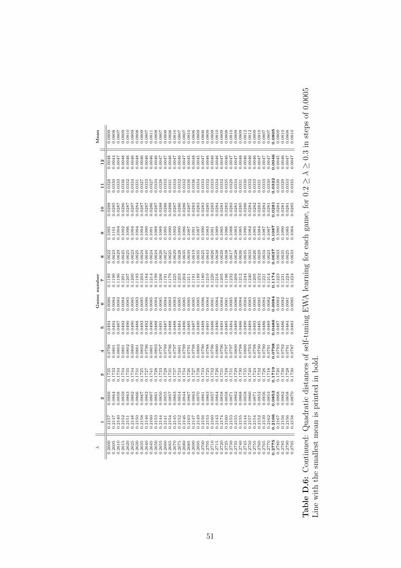
λG

am

enum

ber

Mean

12

34

56

78

910

11

12

0.2600

0.2157

0.0869

0.1735

0.0798

0.0494

0.0086

0.1189

0.0622

0.1095

0.0288

0.0328

0.0048

0.0809

0.2605

0.2147

0.0864

0.1732

0.0801

0.0494

0.0084

0.1190

0.0623

0.1101

0.0285

0.0330

0.0044

0.0808

0.2610

0.2140

0.0858

0.1734

0.0803

0.0487

0.0083

0.1190

0.0629

0.1094

0.0287

0.0333

0.0047

0.0807

0.2615

0.2152

0.0859

0.1734

0.0801

0.0492

0.0084

0.1201

0.0625

0.1092

0.0286

0.0336

0.0048

0.0809

0.2620

0.2151

0.0863

0.1735

0.0802

0.0490

0.0085

0.1207

0.0625

0.1096

0.0287

0.0332

0.0046

0.0810

0.2625

0.2148

0.0862

0.1734

0.0800

0.0490

0.0085

0.1200

0.0623

0.1094

0.0287

0.0334

0.0046

0.0809

0.2630

0.2150

0.0866

0.1731

0.0801

0.0488

0.0083

0.1193

0.0625

0.1094

0.0284

0.0331

0.0048

0.0808

0.2635

0.2158

0.0867

0.1725

0.0802

0.0493

0.0085

0.1203

0.0624

0.1094

0.0287

0.0327

0.0046

0.0809

0.2640

0.2146

0.0862

0.1727

0.0796

0.0492

0.0086

0.1184

0.0640

0.1090

0.0287

0.0333

0.0046

0.0807

0.2645

0.2160

0.0867

0.1741

0.0801

0.0490

0.0085

0.1214

0.0624

0.1091

0.0286

0.0327

0.0046

0.0811

0.2650

0.2153

0.0861

0.1728

0.0803

0.0488

0.0084

0.1199

0.0624

0.1089

0.0287

0.0334

0.0046

0.0808

0.2655

0.2144

0.0850

0.1733

0.0797

0.0491

0.0085

0.1206

0.0626

0.1089

0.0288

0.0328

0.0047

0.0807

0.2660

0.2141

0.0855

0.1728

0.0799

0.0487

0.0084

0.1191

0.0627

0.1095

0.0286

0.0333

0.0047

0.0806

0.2665

0.2154

0.0857

0.1731

0.0796

0.0488

0.0083

0.1179

0.0625

0.1090

0.0288

0.0331

0.0046

0.0806

0.2670

0.2145

0.0863

0.1737

0.0797

0.0488

0.0083

0.1225

0.0629

0.1092

0.0287

0.0334

0.0047

0.0810

0.2675

0.2152

0.0854

0.1724

0.0801

0.0484

0.0085

0.1203

0.0628

0.1090

0.0286

0.0332

0.0046

0.0807

0.2680

0.2146

0.0844

0.1734

0.0799

0.0490

0.0085

0.1204

0.0635

0.1086

0.0286

0.0332

0.0047

0.0807

0.2685

0.2163

0.0867

0.1726

0.0791

0.0485

0.0085

0.1211

0.0639

0.1087

0.0287

0.0336

0.0045

0.0810

0.2690

0.2147

0.0863

0.1727

0.0798

0.0487

0.0085

0.1191

0.0619

0.1091

0.0283

0.0336

0.0048

0.0806

0.2695

0.2149

0.0870

0.1738

0.0800

0.0490

0.0085

0.1189

0.0635

0.1087

0.0283

0.0334

0.0045

0.0809

0.2700

0.2156

0.0861

0.1733

0.0790

0.0488

0.0086

0.1180

0.0625

0.1090

0.0283

0.0333

0.0047

0.0806

0.2705

0.2153

0.0863

0.1725

0.0788

0.0491

0.0084

0.1210

0.0643

0.1083

0.0285

0.0332

0.0046

0.0809

0.2710

0.2160

0.0857

0.1732

0.0796

0.0486

0.0081

0.1220

0.0626

0.1091

0.0283

0.0333

0.0046

0.0809

0.2715

0.2143

0.0864

0.1726

0.0800

0.0490

0.0084

0.1216

0.0638

0.1089

0.0284

0.0334

0.0046

0.0810

0.2720

0.2174

0.0858

0.1731

0.0796

0.0491

0.0084

0.1205

0.0629

0.1085

0.0281

0.0332

0.0047

0.0809

0.2725

0.2160

0.0858

0.1728

0.0797

0.0485

0.0081

0.1196

0.0638

0.1086

0.0283

0.0335

0.0046

0.0808

0.2730

0.2153

0.0871

0.1731

0.0797

0.0484

0.0085

0.1232

0.0617

0.1088

0.0283

0.0329

0.0047

0.0810

0.2735

0.2155

0.0862

0.1729

0.0800

0.0489

0.0086

0.1209

0.0628

0.1083

0.0281

0.0334

0.0047

0.0809

0.2740

0.2155

0.0868

0.1730

0.0798

0.0486

0.0084

0.1212

0.0626

0.1085

0.0285

0.0331

0.0048

0.0809

0.2745

0.2144

0.0858

0.1735

0.0800

0.0490

0.0084

0.1244

0.0635

0.1090

0.0286

0.0330

0.0046

0.0812

0.2750

0.2157

0.0860

0.1740

0.0793

0.0489

0.0083

0.1240

0.0633

0.1084

0.0284

0.0332

0.0046

0.0812

0.2755

0.2154

0.0871

0.1724

0.0798

0.0493

0.0085

0.1205

0.0626

0.1085

0.0282

0.0333

0.0046

0.0809

0.2760

0.2152

0.0852

0.1732

0.0790

0.0485

0.0085

0.1252

0.0629

0.1084

0.0283

0.0331

0.0047

0.0810

0.2765

0.2139

0.0856

0.1726

0.0790

0.0486

0.0084

0.1221

0.0634

0.1087

0.0284

0.0333

0.0047

0.0807

0.2770

0.2162

0.0853

0.1718

0.0791

0.0489

0.0082

0.1214

0.0623

0.1087

0.0281

0.0330

0.0047

0.0807

0.2

775

0.2

166

0.0

853

0.1

719

0.0

798

0.0

486

0.0

084

0.1

174

0.0

637

0.1

087

0.0

281

0.0

332

0.0

046

0.0

805

0.2780

0.2167

0.0868

0.1720

0.0793

0.0487

0.0083

0.1223

0.0633

0.1080

0.0284

0.0330

0.0045

0.0809

0.2785

0.2156

0.0862

0.1730

0.0792

0.0486

0.0082

0.1231

0.0635

0.1090

0.0281

0.0329

0.0046

0.0810

0.2790

0.2156

0.0858

0.1728

0.0791

0.0484

0.0081

0.1224

0.0625

0.1085

0.0281

0.0333

0.0047

0.0808

0.2795

0.2158

0.0870

0.1730

0.0787

0.0483

0.0085

0.1224

0.0633

0.1084

0.0285

0.0335

0.0047

0.0810

Table

D.6

:C

onti

nued

:Q

uad

rati

cdis

tance

sof

self

-tunin

gE

WA

lear

nin

gfo

rea

chga

me,

for

0.2≥λ≥

0.3

inst

eps

of0.

0005

Lin

ew

ith

the

smal

lest

mea

nis

pri

nte

din

bol

d.

51

λG

am

enum

ber

Mean

12

34

56

78

910

11

12

0.2800

0.2166

0.0862

0.1741

0.0792

0.0486

0.0084

0.1243

0.0633

0.1085

0.0280

0.0332

0.0046

0.0812

0.2805

0.2143

0.0857

0.1729

0.0791

0.0485

0.0084

0.1223

0.0623

0.1086

0.0279

0.0335

0.0046

0.0807

0.2810

0.2150

0.0848

0.1730

0.0797

0.0491

0.0081

0.1221

0.0617

0.1087

0.0284

0.0328

0.0048

0.0807

0.2815

0.2161

0.0863

0.1729

0.0789

0.0488

0.0085

0.1233

0.0638

0.1083

0.0282

0.0336

0.0046

0.0811

0.2820

0.2174

0.0868

0.1724

0.0797

0.0491

0.0083

0.1252

0.0629

0.1084

0.0281

0.0334

0.0046

0.0814

0.2825

0.2159

0.0861

0.1730

0.0794

0.0484

0.0082

0.1208

0.0645

0.1090

0.0279

0.0327

0.0046

0.0809

0.2830

0.2157

0.0858

0.1724

0.0796

0.0488

0.0084

0.1259

0.0630

0.1080

0.0280

0.0335

0.0047

0.0812

0.2835

0.2163

0.0866

0.1724

0.0797

0.0486

0.0082

0.1242

0.0624

0.1090

0.0282

0.0337

0.0048

0.0812

0.2840

0.2160

0.0859

0.1722

0.0787

0.0487

0.0085

0.1279

0.0642

0.1086

0.0278

0.0334

0.0046

0.0814

0.2845

0.2159

0.0870

0.1724

0.0799

0.0484

0.0083

0.1257

0.0640

0.1085

0.0281

0.0336

0.0047

0.0814

0.2850

0.2160

0.0854

0.1725

0.0794

0.0490

0.0081

0.1243

0.0629

0.1083

0.0283

0.0336

0.0047

0.0810

0.2855

0.2183

0.0854

0.1717

0.0792

0.0485

0.0083

0.1267

0.0636

0.1081

0.0286

0.0329

0.0047

0.0813

0.2860

0.2162

0.0846

0.1726

0.0790

0.0488

0.0084

0.1247

0.0624

0.1079

0.0280

0.0331

0.0047

0.0809

0.2865

0.2157

0.0866

0.1723

0.0793

0.0490

0.0082

0.1209

0.0637

0.1077

0.0282

0.0337

0.0048

0.0809

0.2870

0.2171

0.0861

0.1730

0.0790

0.0488

0.0083

0.1261

0.0648

0.1081

0.0278

0.0335

0.0047

0.0814

0.2875

0.2175

0.0856

0.1728

0.0785

0.0486

0.0082

0.1233

0.0635

0.1083

0.0281

0.0332

0.0046

0.0810

0.2880

0.2151

0.0873

0.1718

0.0796

0.0486

0.0082

0.1266

0.0646

0.1079

0.0282

0.0332

0.0047

0.0813

0.2885

0.2152

0.0867

0.1724

0.0789

0.0482

0.0082

0.1256

0.0630

0.1085

0.0277

0.0327

0.0048

0.0810

0.2890

0.2154

0.0850

0.1722

0.0791

0.0490

0.0082

0.1280

0.0642

0.1077

0.0280

0.0334

0.0048

0.0813

0.2895

0.2148

0.0859

0.1729

0.0793

0.0484

0.0081

0.1252

0.0632

0.1077

0.0280

0.0335

0.0048

0.0810

0.2900

0.2164

0.0856

0.1720

0.0793

0.0486

0.0083

0.1245

0.0636

0.1077

0.0280

0.0333

0.0048

0.0810

0.2905

0.2152

0.0855

0.1727

0.0785

0.0488

0.0083

0.1273

0.0640

0.1075

0.0282

0.0329

0.0048

0.0811

0.2910

0.2158

0.0868

0.1721

0.0790

0.0492

0.0084

0.1273

0.0628

0.1080

0.0279

0.0334

0.0047

0.0813

0.2915

0.2172

0.0860

0.1730

0.0793

0.0482

0.0084

0.1274

0.0642

0.1082

0.0279

0.0336

0.0046

0.0815

0.2920

0.2154

0.0858

0.1722

0.0787

0.0487

0.0083

0.1264

0.0635

0.1078

0.0281

0.0332

0.0047

0.0811

0.2925

0.2177

0.0853

0.1726

0.0786

0.0488

0.0083

0.1276

0.0645

0.1075

0.0276

0.0335

0.0046

0.0814

0.2930

0.2146

0.0869

0.1726

0.0786

0.0485

0.0082

0.1253

0.0641

0.1075

0.0280

0.0331

0.0048

0.0810

0.2935

0.2157

0.0870

0.1729

0.0787

0.0486

0.0082

0.1297

0.0635

0.1080

0.0279

0.0334

0.0047

0.0815

0.2940

0.2172

0.0871

0.1730

0.0786

0.0486

0.0081

0.1290

0.0650

0.1073

0.0277

0.0336

0.0047

0.0817

0.2945

0.2147

0.0857

0.1728

0.0787

0.0487

0.0081

0.1259

0.0646

0.1075

0.0278

0.0331

0.0048

0.0810

0.2950

0.2165

0.0865

0.1731

0.0791

0.0489

0.0081

0.1261

0.0645

0.1078

0.0280

0.0334

0.0048

0.0814

0.2955

0.2178

0.0850

0.1729

0.0793

0.0484

0.0081

0.1281

0.0646

0.1087

0.0279

0.0333

0.0048

0.0816

0.2960

0.2145

0.0865

0.1723

0.0791

0.0483

0.0082

0.1268

0.0642

0.1079

0.0278

0.0339

0.0048

0.0812

0.2965

0.2153

0.0861

0.1726

0.0786

0.0486

0.0083

0.1241

0.0641

0.1078

0.0276

0.0337

0.0048

0.0810

0.2970

0.2158

0.0856

0.1724

0.0793

0.0490

0.0083

0.1262

0.0648

0.1075

0.0281

0.0331

0.0047

0.0812

0.2975

0.2147

0.0862

0.1725

0.0792

0.0482

0.0083

0.1260

0.0638

0.1085

0.0279

0.0331

0.0048

0.0811

0.2980

0.2188

0.0856

0.1719

0.0787

0.0485

0.0080

0.1279

0.0648

0.1076

0.0279

0.0332

0.0049

0.0815

0.2985

0.2178

0.0860

0.1717

0.0791

0.0486

0.0082

0.1288

0.0646

0.1082

0.0277

0.0334

0.0046

0.0816

0.2990

0.2153

0.0865

0.1731

0.0790

0.0488

0.0080

0.1242

0.0639

0.1079

0.0279

0.0335

0.0048

0.0811

0.2995

0.2160

0.0864

0.1726

0.0789

0.0486

0.0082

0.1287

0.0641

0.1077

0.0281

0.0335

0.0048

0.0815

0.3000

0.2164

0.0862

0.1722

0.0792

0.0483

0.0082

0.1285

0.0649

0.1070

0.0277

0.0334

0.0049

0.0814

Table

D.6

:C

onti

nued

:Q

uad

rati

cdis

tance

sof

self

-tunin

gE

WA

lear

nin

gfo

rea

chga

me,

for

0.2≥λ≥

0.3

inst

eps

of0.

0005

52