Learning from Deregulation:

The Asymmetric Impact of Lockdown and Reopening on Risky Behavior

During COVID-19*

Edward L. Glaeser†, Ginger Zhe Jin‡, Benjamin T. Leyden§, and Michael Luca**

Abstract

During the COVID-19 pandemic, states issued and then rescinded stay-at-home orders that restricted

mobility. We develop a model of learning by deregulation, which predicts that lifting stay-at-home

orders can signal that going out has become safer. Using restaurant activity data, we find that the

implementation of stay-at-home orders initially had a limited impact, but that activity rose quickly after

states’ reopenings. The results suggest that consumers inferred from reopening that it was safer to eat

out. The rational, but mistaken inference that occurs in our model may explain why a sharp rise of

COVID-19 cases followed reopening in some states.

Keywords: coronavirus, COVID-19, public health measures, mobility

* Luca has done consulting for tech companies, including Yelp. Leyden was previously employed as an Economics

Research Intern at Yelp but did not receive compensation directly connected to this paper. † Edward L. Glaeser, Department of Economics, Harvard University, 315A Littauer Center, Cambridge, MA 02138, and NBER, eglaeser@harvard.edu. ‡ Ginger Zhe Jin, Department of Economics, University of Maryland, College Park, MD 20742, and NBER, ginger@umd.edu. § Benjamin T. Leyden, Dyson School of Applied Economics and Management, Cornell University, 376D Warren Hall, Ithaca, NY 14853, and CESifo, leyden@cornell.edu. ** Michael Luca, Harvard Business School, Harvard University, Soldiers Field, Boston, MA 02163, and NBER, mluca@hbs.edu.

1

1. INTRODUCTION

Governments sometimes go so far as to ban an activity that is deemed sufficiently unsafe, at

least until the perceived risk has sufficiently abated. Beaches are closed when sharks are spotted in

the water, restaurants with unclean food practices are shuttered, and, in the spring of 2020, whole

states and countries were essentially shut down because of fear of COVID-19.

Lifting these bans can have both a direct effect—people who always wanted to do the activity

can do so—and an indirect effect—the lifting of the regulation sends a signal suggesting that the

activity is now safe. We refer to this signaling effect as learning from deregulation. In this paper, we

develop a model of learning from deregulation and test the model’s predictions about restaurant

visits before and after COVID-19 lockdown periods.

Our model is motivated by the basic course of COVID-19. Beginning in March 2020, states and

cities around the United States issued stay-at-home orders that restricted mobility and lasted for

months. Data from SafeGraph and Yelp shows that people had largely stopped eating in restaurants

before the local lockdowns took effect. Indeed, once we control for nationwide trends, the onset of

local regulation had almost no impact, which has led some to argue that the lockdowns had no effect

on behavior (Goolsbee & Syverson, 2021; Gupta et al., 2020).

PLACE FIGURE 1 HERE

Extending the data through the end of the regulatory lockdown, we observe an asymmetric

response to reopening, where restaurant visits spiked shortly after state governments allowed

restaurants to reopen for dine-in service. As Figure 1 shows, the public radically reduced restaurant

visits before lockdown orders were issued, but reopening was immediately followed by sharp

increases in eating out. Why would the impact of ending a regulation be larger in magnitude than the

impact of imposing the regulation?

2

Standard static models of regulation and behavior suggest a symmetry between the imposition

and the elimination of a restriction, but that symmetry ends if restricting behavior also reduces the

flow of information about that behavior. Section II presents a simple dynamic signaling model,

where the public had information about safety before closing, but not before reopening.

Consequently, there is no signaling impact of closing, but if the government has private information

about risk then reopening provides a signal of safety.

In the model, consumers take an action, such as dining out, that is normally safe, but has

temporarily become risky. Both the government and consumers learn about the onset of the risk

simultaneously, which first leads consumers to reduce their activity and then leads the government

to impose a lockdown. By assumption, consumers move first because dining in takes less time than

crafting an executive order. Once the shutdown order occurs, consumers lose their direct source of

information about the risk, but the government receives a private signal about safety and decides

whether to reopen the economy.

We show that there exists a separating or semi-pooling equilibrium where the reopening decision

signals that the world has become safer, which then triggers a positive consumer response to

reopening. If politicians are risk-averse, perhaps because they have a relatively high probability of

reelection, then the equilibrium is separating and reopening perfectly signals safety. If some

governments are risk-loving, perhaps because their re-election is a long shot, then governments with

an adverse signal may pool with governments that receive a positive signal. In that case, reopening

can lead to harm because consumers interpret reopening to suggest greater safety than is the case.

After developing this model, we then explore the model’s testable implications in the data. In

Section III, we discuss our data sources from SafeGraph and Yelp. In Section IV, we present our

results on the asymmetric impact of the lockdowns and reopenings. In this section, we also estimate

the interaction between re-opening and the Republican vote share in the 2016 general election,

3

which we interpret as an indication of optimism about safety. Additionally, we show the relationship

between the timing of reopening and post-reopening COVID-19 rates, which suggests that

consumers interpreted reopening to imply less risk than there was in reality. Section V concludes.

Neither the model nor our empirical work suggests that reopening was necessarily a good or bad

decision, but it does suggest consumers interpreted states’ reopening decisions as a signal that the

risk had abated, even in states where that does not appear to have been the case.

2. A SIMPLE MODEL OF BELIEFS AND REGULATORY REOPENING

This paper focuses on a simple, common hypothesis: consumers believe that the end of a

regulatory lockdown signifies that they can safely return to their interactive activities. To make sense

of this belief, and of why it might occasionally be incorrect, we investigate a simple, stylized model

of a government that chooses whether or not to end a regulatory ban in the presence of private

information. We treat this as a game between a unitary decision-maker (the government) and non-

strategic consumers, who undertake an action if they believe that the risk associated with that action

is less costly than the reward. We will describe the sequence of events before the reopening decision

and explain why they are consistent with our assumptions about the actors’ behaviors, and then

characterize the Bayesian Nash equilibrium in the reopening game between government and

consumers.

2.1 Model setup

Individuals can take a potentially risky action “A,” such as going to a restaurant. The net flow

benefit from the action is denoted 𝐵𝑖 > 0 and we abstract away from non-health related costs. The

distribution of benefits is characterized by a cumulative distribution function F(B) and related

density f(B). Taking the action creates a risk of harm which is unknown, time changing and denoted

4

𝜋𝑡. Consumers’ expected value of 𝜋𝑡 at the start of period t is 𝜋⏞𝑡. The private cost of harm equals C

and the social cost of harm equals 𝐶 + ∆. The share of individuals who will undertake the action,

unless there is a public lockdown, equals 1 − 𝐹(𝜋⏞𝑡 𝐶). If there is a lockdown, then no one

undertakes the action. The social costs of harm will also be spread across consumers, but those costs

will not influence behavior.

While the action in this model could refer to going to a restaurant, and the harm could be

catching a contagious disease, this model can also describe other settings where governments ban

activities. For example, the government can ban swimming because of either rough waves or sharks,

or the government can ban a restaurant because of food poisoning. We assume that the

government’s policy toolkit is particularly limited: it can either ban the action or not.

At the period of reopening, the government’s objective function is the expected value of

𝐺(𝐴𝑣𝑒𝑟𝑎𝑔𝑒 𝐶𝑜𝑛𝑠𝑢𝑚𝑒𝑟 𝑊𝑒𝑙𝑓𝑎𝑟𝑒 − 𝑆𝑜𝑐𝑖𝑎𝑙 𝐶𝑜𝑠𝑡 𝑜𝑓 𝐻𝑎𝑟𝑚), where 𝐺(𝑥) = 𝑥 + 𝛼|𝑥|. The

function G(.) is concave around zero if 𝛼 < 0 and convex if 𝛼 > 0. We assume that −1 < 𝛼 < 1,

so that the function is always monotonic. The 𝛼 term can generate a divergence between the

government’s reopening decision and the socially optimal reopening decision, because the

government behavior is either more risk averse or risk loving than the public at large. We assume

that 𝛼 is known to the public. We interpret this parameter as a reflection of political incentives

rather than deep preferences. For example, the governmental leader might ultimately care about re-

election, as is the norm in political economy models of career concerns (e.g. Besley, 2007). If the

politician is headed towards an easy victory, then 𝛼 < 0 because added volatility will increase the

possibility of losing power. If the politician is likely to lose office without some major success, then

𝛼 > 0.

5

The value of 𝜋𝑡 is either 𝜋 or 𝜋. The state is always observed accurately by the public at the end

of each period if consumption is allowed. When consumption is not allowed, we assume that the

government receives a private signal of the state of the world. The probability transitions from 𝜋𝑡 =

𝜋 to 𝜋𝑡 = 𝜋 with probability 𝛿𝑂 ≈ 0 and from 𝜋𝑡 = 𝜋 to 𝜋𝑡 = 𝜋 with probability 𝛿 < .5. We treat

𝛿𝑂 = 0 to capture the highly unexpected nature of the emergence of the high-risk state.

2.2 Timing

We assume the following sequence of events. At time t=-2, the state of the world changed from

𝜋𝑡 = 𝜋 to 𝜋𝑡 = 𝜋, and this change was observed at the start of period t=-1. Consequently, demand

fell from 1 − 𝐹(𝜋 𝐶) to 1 − 𝐹(( 𝛿𝜋 + (1 − 𝛿)𝜋)𝐶) between periods -2 and -1. The government

then imposed a ban on the action that caused the level of activity to fall to zero at time t=0.

Why did the government wait a time period, and why did a ban maximize the government’s

welfare? We assume that the time delay was technological, and that the government could not

immediately institute a ban. We also assume either that the government solved a dynamic

programming problem and determined that the ban was in its interests, or that external forces

induced the government to undertake the ban. We are not interested in that initial decision, and so

we will not microfound the government’s optimization problem at the point of the initial ban.

Instead, we are interested in the government’s decision to reopen, which will allow the action to

be taken at t=1. We assume that after t=1, the game ends. Consumers have no direct information on

the risks of the action, because the action has been shut down, but do know the government’s

objective function, transition probabilities, and that 𝜋−1 = 𝜋. We further assume that the

government has access to a private signal that informs it of the state of the world as of time t=0.

2.3 Equilibrium

6

We define a Bayesian equilibrium in this setting as one in which (1) if the government reopens,

then consumers’ believe that the probability of harm 𝜋⏞1 satisfies Bayes’ rule so that 𝜋⏞1 =

𝛿𝑃𝐿𝑜𝑤 𝑅𝑖𝑠𝑘𝑅𝑒𝑜𝑝𝑒𝑛

+(1−𝛿)𝛿𝑃𝐻𝑖𝑔ℎ 𝑅𝑖𝑠𝑘𝑅𝑒𝑜𝑝𝑒𝑛

𝛿𝑃𝐿𝑜𝑤 𝑅𝑖𝑠𝑘𝑅𝑒𝑜𝑝𝑒𝑛

+(1−𝛿)𝑃𝐻𝑖𝑔ℎ 𝑅𝑖𝑠𝑘𝑅𝑒𝑜𝑝𝑒𝑛 , where 𝑃𝐿𝑜𝑤 𝑅𝑖𝑠𝑘

𝑅𝑒𝑜𝑝𝑒𝑛 and 𝑃𝐻𝑖𝑔ℎ 𝑅𝑖𝑠𝑘

𝑅𝑒𝑜𝑝𝑒𝑛 reflect the probability that the government

will reopen conditional upon receiving a low risk or high risk signal (with probability 𝛿, a high risk

situation becomes low risk in the next period, and the situation was high risk at t=-1), (2) consumer

demand equals 1 − 𝐹(𝜋⏞1 𝐶), (3) the government always opens if the expectation of its payoff upon

reopening is higher than zero, never opens if it is lower than zero, and may randomize between

opening and reopening if its expected payoff conditional upon reopening equals zero.

We also assume that B is uniformly distributed on the unit interval, so that average social welfare

less social cost of harm equals (1 − 𝜋⏞1 𝐶) (1+𝜋⏞1 𝐶

2− 𝜋(𝐶 + ∆)) if risk is low and known to be low

and (1 − 𝜋⏞1 𝐶) (1+𝜋⏞1 𝐶

2− 𝜋(𝐶 + ∆)) if the risk is high. We assume that

1

𝜋> 2∆ + 𝐶 >

1

(1−𝛿)𝜋+𝛿𝜋,

which ensures that the net social welfare from allowing the action is negative if risks were high last

period. This assumption helps justify why the prohibition was instituted in the first place.i

The following proposition refers to high demand as the demand at time -2 (i.e. 1 − 𝜋 𝐶) and low

demand as the demand if there is no information content from reopening (i.e. 1 − 𝐶((1 − 𝛿)2𝜋 +

(2 − 𝛿)𝛿𝜋)), which equals the demand before closing if 𝛿 = 0. We identify low demand after

reopening with a symmetric response to opening and closing and high demand after reopening as an

asymmetric response.

Proposition 1: There exist two values 𝛼2 > 𝛼1 > 0, so that if 𝛼1 > 𝛼, then the public sector

only reopens if the risk fell in period 0, and in that case, there is high demand after reopening. If

𝛼 > 𝛼2, then the government always reopens and there is low demand after reopening. If 𝛼2 > 𝛼 >

7

𝛼1, there are three possible Bayesian equilibrium: (1) the government always reopens and there is

low demand after reopening, (2) the government reopens only if the risk has declined and there is

high demand after reopening and (3) the government always reopens if the risk has declined and

sometimes reopens if the risk has not declined, and in this semi-pooling equilibrium, the demand

after reopening lies between high and low demand and is increasing with 𝛿, and decreasing with 𝛼,

∆, C, 𝜋, and 𝜋.

.

Proposition 1 predicts that symmetry occurs in a pooling equilibrium, where there is no new

information from the act of reopening, or if the government had no information. If the government

has information and opens only when it has learned that conditions have shifted to safety, then the

proposition predicts asymmetry. The fundamental difference between opening and closing is that

when the action is ongoing, the consumer knows as much as the government. During lockdown, the

government continues to receive a signal while consumers do not. Thus, consumers rely on the

reopening decision to learn the state of the world. However, when there is semi-pooling, that

inference will be imperfect, though it still is positive and produces some demand response to

reopening. Unless there is complete pooling, there will be an asymmetric response to reopening,

relative to the initial closing, because reopening generates some information.

The model also predicts that if the disease was thought to be less harmful, because either C or 𝜋

or 𝜋 are lower, then the response to reopening will be larger in a semi-pooling equilibrium. This is

not so much a reflection of signaling, but rather that these variables capture the expected harm from

reopening as long as there is some chance that the risk level is high. A higher value of 𝛿 increases

demand in a semi-pooling equilibrium, because it increases the chances that the high-risk situation

has evolved into a low risk situation. Higher values of 𝛼 imply more pooling, which generate weaker

demand, and low values of 𝛼 imply separating, which will generate strong demand.

8

While the model is framed around a single action, it could easily be modified to allow multiple

actions, all of which generate risk that depends on the state of the world. The asymmetry should

appear most stark in those activities that are most dependent upon the perceived state of the world.

For example, visits to a park or an open beach would, independent of whether or not the world is

high risk, experience a more symmetric effect of the lockdown and reopening. Restaurants visits,

which present greater risks than more general activity, would be expected to exhibit a more

asymmetric reopening effect, if reopening is taken to mean that the risk is lower.

Even within restaurant visits, one would expect variation in the asymmetry of the response. For

example, if there were some restaurants that were known to provide safety through social distancing,

or if some restaurants only provided take-out service, then those restaurants should experience a

more symmetric effect of the lockdown and the reopening than restaurants that primarily offer

indoors, dine-in service.

3. SAFEGRAPH AND YELP DATA BEFORE AND AFTER STAY-AT-HOME

REGULATIONS

We construct a daily, state-level time series for six measures of mobility and restaurant activities

using cell phone location data from the geospatial data company SafeGraphii and the online review

platform Yelp. Our data range from December 1, 2019 to June 14, 2020. Due to the proprietary

nature of our data from Yelp, all of our measures of mobility and restaurant activities are calculated

relative to a state's December 2019 daily average. For example, a value of 0.75 indicates a 25%

reduction in activity relative to the December 2019 daily average.

First, to understand how states' lockdown and reopening orders affected general mobility, we

construct an "All Visits" measure, which uses SafeGraph's geospatial data to count the number of

daily visits to all places-of-interest within a state. We then construct two mobility measures related to

9

restaurant activity. The first, "Restaurant Visits" measures the total number of visits to all restaurants

and other food-service locations. The second, "Full-Service Restaurant Visits" further restricts this

sample to only those businesses classified by NAICS as full-service restaurants; cafeterias, grill

buffets and buffets; or drinking places (alcoholic beverages).iii

PLACE TABLE 1 HERE

We present summary statistics for these three measures of mobility in Table 1. Of primary

relevance to our analysis is how these measures changed around the states’ stay-at-home and

reopening orders. To illustrate these changes, we calculate ΔStay Home and ΔReopen, as the

difference between the average value of each measure in the week after and the week before an

order was issued. We present the mean and standard deviation of these differences in the last four

columns of Table 1. As expected, we see evidence of a decline in mobility after the issuance of a

stay-at-home order, and an increase in mobility following reopening decisions. Notably, the change

in mobility around reopening, relative to the decline in mobility around the stay-at-home order is

increasing in the relative risk of the activity, as we move from general mobility ("All Visits") to

visiting a full-service restaurant (“Full-Service Restaurant Visits”).

We next construct three measures of restaurant activity using data from Yelp. First, we use data

from the Yelp Reservations platform to understand how people's willingness to dine at a restaurant

changes in response to the COVID-19 pandemic, and states' local orders. This measure represents

the total number of reservations scheduled to occur on a given date.iv Second, we use data from the

Yelp Transactions Platform, which allows users to place delivery and takeout orders with local

restaurants, to construct our "Orders" sample. Our final measure of restaurant activity is our "Page

Views" sample, which totals the number of restaurant page views online or via mobile apps. We take

this as a measure of user intent—to visit or order from a restaurant.

10

Summary statistics for each of these three measures are presented in Table 1. Similar to the Full-

Service Restaurant Visits measure from the SafeGraph data, we see initial evidence of a decline in

reservations and page views at the time of shutdown, and a relatively large increase in activity at the

time of the shutdown, consistent with the asymmetric response predicted by our model. The Orders

sample, however, shows a different response. On average, we see an increase in the number of

delivery and takeout orders in the week following the issuance of a stay-at-home orderv, although, as

illustrated in Figure 1a, this reflects a general upward trend that predates stay-at-home orders.

In comparison, it is difficult to tell whether the response to lockdown and reopening is

symmetric from macro data. According to the U.S. Census Monthly Retail Trade reportsvi, total retail

and food services have dropped in March (-8.22% from previous month) and April (-14.71%) but

increased in May (18.16%) and June (7.50%). The month-to-month changes on food services and

drinking places are of greater magnitudes, namely -30.04% and -34.32% in March and April,

and +31.55% and +20.04% in May and June. While the percentage changes seem comparable before

and after April, the absolute terms tell a different story. According to the National Restaurant

Association, although June 2020 represented the highest monthly sales volume since the beginning

of the pandemic lockdowns in March, it still remained roughly $18 billion (27.6%) down from the

pre-coronavirus sales levels posted in January and February.vii These macro statistics differ from our

data, because they tend to reflect national changes and do not account for the timing of local

lockdown and reopening orders.

In addition to the mobility and restaurant activity measures described above, we also use data on

COVID-19 penetration, and the vote share for the Republican candidate in the 2016 presidential

election. To measure COVID-19 penetration, we collect daily, cumulative COVID-19 case counts

from New York Timesviii and the vote share data from Townhall.com.ix Finally, we identified the

11

date of each state's stay-at-home and reopening orders from a combination of local news reports

and official government documentation.x Since states typically adopted a multi-phase approach to

reopening, we classify a state as having reopened on the first date that restaurants were permitted to

serve customers on premises (either indoors or outdoors).

4. THE ASYMMETRIC IMPACT OF STARTING AND ENDING LOCKDOWN

POLICIES

In this section, we first document an asymmetric response to states' stay-at-home orders across

all six of our measures of mobility and restaurant activity. We then explore two implications of our

model: 1) that the asymmetry should appear larger in activities that are most dependent on the

perceived amount of risk in going out, and 2) that there is a larger reopening response under a semi-

pooling equilibrium when the population believes that the virus risk is lower. Following that, we

consider the role of publicly available information about COVID-19 cases in the public’s daily

behavior. Finally, we provide suggestive evidence that some states are indeed in the semi-pooling

equilibrium described in Proposition 1.

4.1 Empirical specification

To document the asymmetric response to states' shutdown and reopening orders, we estimate

the following regression equation,

𝑦𝑠,𝑡 = 𝛼 + 𝛽11(𝑆𝑡𝑎𝑦 𝐻𝑜𝑚𝑒)𝑠,𝑡 + 𝛽21(𝑅𝑒𝑜𝑝𝑒𝑛)𝑠,𝑡 + 𝛾11(𝑁𝑜 𝐶𝑜𝑣𝑖𝑑)𝑠,𝑡 + 𝛾2𝑅𝑒𝑙. 𝐶𝑜𝑣𝑖𝑑𝑠,𝑡

+𝛿𝑠 + 𝛿𝑡 + 𝜖𝑠,𝑡 .

12

Where 𝑦𝑠,𝑡 is the outcome of interest for state 𝑠 on day 𝑡, and 1(𝑆𝑡𝑎𝑦 𝐻𝑜𝑚𝑒)𝑠,𝑡 and

1(𝑅𝑒𝑜𝑝𝑒𝑛)𝑠,𝑡 are indicators for whether the state was under a stay-at-home or reopening order on

day 𝑡. To account for COVID-19 penetration, we include a control equal to one if the state has not

disclosed the number of COVID-19 cases by day 𝑡, 1(𝑁𝑜 𝐶𝑜𝑣𝑖𝑑)𝑠,𝑡, and a relative measure of

COVID-19 if the information on COVID-19 cases is available, 𝑅𝑒𝑙. 𝐶𝑜𝑣𝑖𝑑𝑠,𝑡.

More specifically, to construct 𝑅𝑒𝑙. 𝐶𝑜𝑣𝑖𝑑𝑠,𝑡, we first compute a state’s total number of

COVID-19 cases per million population as of day t, and then divide it by the nationwide number of

COVID-19 cases per million population on the same day. xi We use this relative measure because the

absolute number of COVID-19 cases follows a similar trend in many states and the relative measure

emphasizes the heterogeneity of state experiences. Finally, we include state and day fixed effects, 𝛿𝑠

and 𝛿𝑡.

We consider three mobility outcomes: all visits to places-of-interest, visits to all restaurants, and

visits to full-service restaurants, using data from SafeGraph, a geospatial data company. Additionally,

we consider three measures from Yelp, the online review platform, which are more closely linked to

restaurant activity: reservations, takeout and delivery orders, and the number of page views for

restaurants’ Yelp listings. These outcomes are discussed in more detail in Section III.

4.2 Results

PLACE TABLE 2 HERE

Table 2 shows that all six of our outcomes of mobility and restaurant activity display an

asymmetric response to regulation. There is little or no response to the states' initial shutdown

orders. The largest response is a 2.6 percentage point reduction in our SafeGraph measure of visits

to all places-of-interest. We find no evidence of a response to stay-at-home orders across all three

13

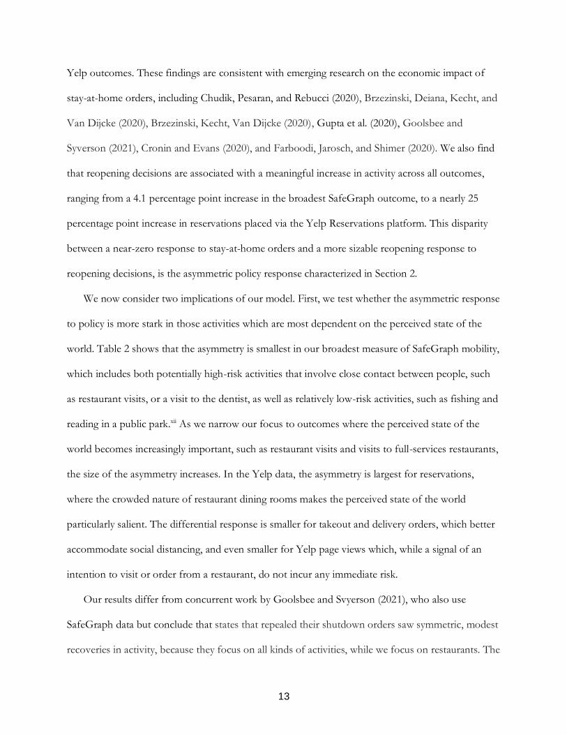
Yelp outcomes. These findings are consistent with emerging research on the economic impact of

stay-at-home orders, including Chudik, Pesaran, and Rebucci (2020), Brzezinski, Deiana, Kecht, and

Van Dijcke (2020), Brzezinski, Kecht, Van Dijcke (2020), Gupta et al. (2020), Goolsbee and

Syverson (2021), Cronin and Evans (2020), and Farboodi, Jarosch, and Shimer (2020). We also find

that reopening decisions are associated with a meaningful increase in activity across all outcomes,

ranging from a 4.1 percentage point increase in the broadest SafeGraph outcome, to a nearly 25

percentage point increase in reservations placed via the Yelp Reservations platform. This disparity

between a near-zero response to stay-at-home orders and a more sizable reopening response to

reopening decisions, is the asymmetric policy response characterized in Section 2.

We now consider two implications of our model. First, we test whether the asymmetric response

to policy is more stark in those activities which are most dependent on the perceived state of the

world. Table 2 shows that the asymmetry is smallest in our broadest measure of SafeGraph mobility,

which includes both potentially high-risk activities that involve close contact between people, such

as restaurant visits, or a visit to the dentist, as well as relatively low-risk activities, such as fishing and

reading in a public park.xii As we narrow our focus to outcomes where the perceived state of the

world becomes increasingly important, such as restaurant visits and visits to full-services restaurants,

the size of the asymmetry increases. In the Yelp data, the asymmetry is largest for reservations,

where the crowded nature of restaurant dining rooms makes the perceived state of the world

particularly salient. The differential response is smaller for takeout and delivery orders, which better

accommodate social distancing, and even smaller for Yelp page views which, while a signal of an

intention to visit or order from a restaurant, do not incur any immediate risk.

Our results differ from concurrent work by Goolsbee and Svyerson (2021), who also use

SafeGraph data but conclude that states that repealed their shutdown orders saw symmetric, modest

recoveries in activity, because they focus on all kinds of activities, while we focus on restaurants. The

14

asymmetry is more pronounced when looking at riskier activities, which are captured by full-service

restaurants and reservations.

A second implication of our model is that in a semi-pooling equilibrium, demand after a state

reopens will be decreasing with perceived risk of contagion. In the U.S., optimism about COVID-

19, at least during the lockdown phase, was strongly associated with political party. On April 16,

2020, seventy-three percent of Democrats told Gallup Pollsters that they were somewhat or very

worried about catching COVID-19.xiii Only thirty-six percent of Republicans told Gallup that they

were worried about the disease. This difference across parties persisted throughout the shutdown

period, with eighty-five percent of Democrats and only forty-seven percent of Republicans telling

Gallup Pollsters that they were somewhat or very worried about being exposed to coronavirus.xiv

Allcott et al. (2020) show that locations with a greater number of Republicans were less likely to

engage in social distancing. They also present survey results that indicate more conservative

individuals anticipated fewer new cases than more left-leaning individuals. In light of these

differences in perceived risk by political party, we use the 2016 Republican presidential vote share as

a proxy for lower values of �̅�.

PLACE TABLE 3 HERE

In columns 1-4 of Table 3, we interact a normalized measure of each state's 2016 GOP

presidential vote share with the indicators for the stay-at-home and reopening orders. In all three

measures of restaurant visits, SafeGraph's Restaurants and Full-Service Restaurants measures, and

Yelp's Reservations measure, we find that the asymmetry is increasing in GOP vote share. Indeed,

the size of the asymmetry nearly doubles in the Full-Service and Reservations measures when

moving from a state with an average level of 2016 GOP support, say Arizona or North Carolina, to

a state one standard deviation above the mean, such as Nebraska. The one exception, though, is

with Yelp Orders, where there is a larger increase in orders when stay-at-home directives went into

15

effect, but we find no evidence of a relationship between GOP vote share and the reopening

response. Our finding is consistent with Engle, Stromme and Zhou (2020), who only examine the

effect of stay-at-home order and find the order reduces mobility more in the counties that vote less

for the Republican Party in the 2016 presidential election.

Our model does not predict how restaurant activities should vary by the severity of COVID-19

risk throughout the shutdown, because it assumes the public receives no information about the risk

during shutdown. In reality, COVID-19 information is updated daily, although different government

agencies give different interpretations. For this reason, we treat 1(𝑁𝑜 𝐶𝑜𝑣𝑖𝑑)𝑠,𝑡 and 𝑅𝑒𝑙. 𝐶𝑜𝑣𝑖𝑑𝑠,𝑡

as pure controls. The baseline results (Table 2) suggest that a state’s relative severity of COVID-19

risk has little effect on five of the six outcome variables. The only outcome that declines with

relative Covid cases with a marginal significance is SafeGraph mobility to all restaurants.

In columns 5-8 of Table 3, we present two additional interactions between our relative COVID-

19 cases and the indicators for the stay-at-home and reopening orders. During the stay-at-home

period, mobility to all restaurants and online orders from Yelp decline with the COVID-19 risk. The

other two outcomes, mobility to full-service restaurants and Yelp reservations, are insensitive to

𝑅𝑒𝑙. 𝐶𝑜𝑣𝑖𝑑𝑠,𝑡 during shutdown. They already declined to a very low level at the beginning of

shutdown. All four outcomes respond positively to reopening, but these positive responses are

attenuated significantly in regions with higher values of relative COVID-19 cases. This suggests that,

while the public may interpret the government’s reopening order as a signal of safety, they also

incorporate the ongoing information of COVID-19 in their daily behavior.

We now measure the relationship between the timing of reopening, and post-reopening

COVID-19 rates. Under the semi-pooling equilibrium described in Proposition 1, some states will

reopen after receiving a positive private signal, while others will reopen despite having not received a

good signal. In that equilibrium, consumers will be unable to distinguish between these two sets of

16

states, and so may infer from reopening that activity in their state is less risky than it actually is. If

states are in fact in a semi-pooling equilibrium, there should be a greater acceleration of COVID-19

cases in states that opened without a positive signal of safety.

To investigate this, we construct two measures to proxy for states’ private signals, both of which

are based on changes in the rate of COVID-19 cases over time. Our first measure compares the

growth rate of COVID-19 cases one week before the lockdown ends with the growth rate one week

after states make their reopening decision. The growth rate one week after the lockdown ends

should not reflect the reopening itself, which typically would impact cases after at least one week,

but it could reflect private information possessed by the government. We segment states into two

groups based on this measure: “Good Signal” states are those for which the growth rate falls around

the reopening date, and “Bad Signal” states are those for which the growth rate increases around the

reopening date.

As a second measure of private information: the growth in the number of cases two weeks

before reopening relative to one week before reopening. While those cases could be seen by the

public, for many citizens, their meaning may be opaque, and they may believe that the government is

better at interpreting the meaning of those cases for restaurant safety.

PLACE FIGURE 2 HERE

In Figure 2, we plot the average growth rate of COVID-19 cases and the average number of

daily visits to full-service restaurants, both relative to the growth rate on the date of reopening.

Figure 2a employs the private signal proxy that is centered around the reopening date, and Figure 2b

uses the proxy centered around a week before reopening. In both cases, our measure of the

governmental signal strongly predicts the ex-post COVID-19 cases. We interpret this to suggest that

some state governments chose to reopen, despite not receiving a positive signal about safety.

Notably, consumers still interpreted reopening as a positive signal, regardless of which type of state

17

they reside in, as restaurant activity increased across the board, and showed no evidence of a

divergence in trend.

Our results do not imply that it was wrong to reopen, but just that reopening can have a

different impact on behavior than an initial restriction. Some consumers appear to interpret

reopening as a signal that activity is safe.

5. CONCLUSION

Overall, our results help to shed light on the impact of imposing and rescinding stay-at-home

orders throughout much of the United States in the COVID-19 pandemic. Our model highlights

that government actions can have both a direct effect (preventing people who want to go out from

doing so) and an indirect effect (signaling to people when it is safe to go out again).

We then turn to the data, exploring the evolution of restaurant demand before, during, and after

the lockdowns. Consistent with other emerging results, we find that most of the demand had already

dropped before the lockdowns were in place. This suggests that the direct effect of lockdowns was

small in the beginning and has led some policymakers to question the importance of the lockdowns.

However, we also show that demand increases sharply shortly after the end of lockdowns—

suggesting that the lockdowns were in fact relevant by the end. The observed asymmetry and timing

of demand increases are consistent with the signaling mechanism proposed in the model.

Our analysis also shows heterogeneity in demand responses after the end of lockdowns,

associated with political preferences and with the number of COVID-19 cases in an area. Within the

United States, there has been an important partisan component to beliefs about COVID-19, with

Republican-leaning citizens less likely to express concern about the virus. Consistent with this, we

find larger increases in demand in areas with a higher Republican vote share. We also find smaller

jumps in demand in areas with more cumulative COVID-19 cases.

18

Our work has implications for policymakers as well. As Gans (2020) notes, one “key to making

people safe is knowledge.” While some of this knowledge comes in the form of official guidelines

and other direct information, there is also information conveyed through policymakers’ regulatory

decisions. Our work explores the signal value and information being conveyed through a regulatory

decision and highlights the importance for policymakers of accounting for the signal being sent by

the imposition and lifting of bans, such as the COVID-19 stay-at-home orders.

19

Acknowledgements

We thank the editor and anonymous referee for their helpful comments. We thank Safegraph and Yelp for

providing data. We thank Scott Kominers for helpful comments.

References

Allcott, H., Boxell, L., Conway, J., Gentzkow, M., Thaler, M., & Yang, D. (2020). Polarization and

public health: Partisan differences in social distancing during the coronavirus pandemic. Journal of

Public Economics, 104254. https://doi.org/10.1016/j.jpubeco.2020.104254

Besley, T. (2007). Principled Agents?: The Political Economy of Good Government (The Lindahl

Lectures). Oxford University Press.

Brzezinski, A, Deiana, G., Kecht, V., & Van Dijcke, D. (2020). The COVID-19 Pandemic:

Government vs. Community Action Across the United States. Covid Economics: Vetted and Real-

Time Papers 7 (CEPR), 115–156. https://cepr.org/sites/default/files/news/CovidEconomics7.pdf

Brzezinski, Adam, Kecht, V., & Van Dijcke, D. (2020). The Cost of Staying Open: Voluntary Social

Distancing and Lockdowns in the US. SSRN Electronic Journal.

https://doi.org/10.2139/ssrn.3614494

Chudik, A., Pesaran, M. H., & Rebucci, A. (2020). Voluntary and Mandatory Social Distancing:

Evidence on COVID-19 Exposure Rates from Chinese Provinces and Selected Countries. SSRN

Electronic Journal. https://doi.org/10.2139/ssrn.3576703

Couture, V., Dingel, J. I., Green, A., Handbury, J., & Williams, K. R. (2021). JUE Insight: Measuring

movement and social contact with smartphone data: a real-time application to COVID-19. Journal

of Urban Economics, 103328. https://doi.org/10.1016/j.jue.2021.103328

Cronin, C. J., & Evans, W. N. (2020). Private Precaution and Public Restrictions: What Drives Social

Distancing and Industry Foot Traffic in The Covid-19 Era? NBER Working Paper No. 27531.

20

Engle, S., Stromme, J., & Zhou, A. (2020). Staying at Home: Mobility Effects of COVID-19. Covid

Economics 4 (CEPR). https://doi.org/10.2139/ssrn.3565703

Farboodi, M., Jarosch, G., & Shimer, R. (2020). Internal and External Effects of Social Distancing in

a Pandemic. NBER Working Paper No. 27059.

Gans, J. (2020). Economics in the Age of COVID-19 (MIT Press First Reads). The MIT Press.

Goolsbee, A., & Syverson, C. (2021). Fear, lockdown, and diversion: Comparing drivers of

pandemic economic decline 2020. Journal of Public Economics, 104311.

https://doi.org/10.1016/j.jpubeco.2020.104311

Gupta, S., Nguyen, T. D., Rojas, F. L., Raman, S., Lee, B., Bento, A., Simon, K. I., & Wing, C.

(2020). Tracking Public and Private Responses to the COVID-19 Epidemic: Evidence from State

and Local Government Actions. NBER Working Paper No. 27027.

Raj, M., Sundararajan, A., & You, C. (2020). COVID-19 and Digital Resilience: Evidence from Uber

Eats. SSRN Electronic Journal. https://doi.org/10.2139/ssrn.3625638

i While that condition ensures that banning the action is optimal during that one period, it does not imply that the ban

was dynamically optimal since the ban creates the scope for distortionary public action because of its private

information.

ii Many COVID-19 research cited in this paper use cell phone tracking data from Safegraph, Unacast or other

companies. Couture, Dingel, Green, Hanbury, and Williams (2021) compare smartphone data with conventional survey

data such as the Census’s estimated 2019 residential population, the 2014-2018 American Community Survey, the 2017-

2018 IRS Migration Data, and the 2017 National Household Transportation Survey (NHTS). They show that

smartphone data cover a significant fraction of the US population and are broadly representative of the general

population in terms of residential characteristics and movement patterns.

iii These corresponding NAICS codes are 722511, 722514, 722410. Restaurants not included in our definition of full-

service restaurants are limited-service restaurants (NAICS=722513) and snack and nonalcoholic beverage bars

(NAICS=722515).

21

iv We exclude nine states from the Reservations measure, because the platform’s coverage is relatively low in those states.

The states are: AL, AR, DE, MS, ND, OK, RI, SD, WY.

v This finding is consistent with Raj, Sundararajan, and You (2020), who document the increase of online orders on Uber

Eats after stay-at-home orders.

vi https://www.census.gov/retail/marts/www/timeseries.html.

vii https://restaurant.org/articles/news/restaurant-sales-hit-a-pandemic-high-in-june, National Restaurant Association.

viii We use the New York Times data posted at https://github.com/midas-network/COVID-

19/tree/master/data/cases/united%20states%20of%20america/nytimes_covid19_data/.

ix Townhall.com published the 2016 general election results at https://townhall.com/election/2016/president/. We

access county-level data from Townhall.com at https://github.com/tonmcg/US_County_Level_Election_Results_08-

16 and aggregate it into states.

x There was considerable variation in the timing of stay-at-home and reopening orders by state, with stay-at-home orders

ranging from March 17 (CA) to April 7 (SC), and restaurant reopenings ranging from April 24 (AK) to June 15 (NJ).

xi We use the 2019 state population as estimated by the US Census Bureau, accessed at

https://www.census.gov/data/tables/time-series/demo/popest/2010s-state-total.html.

xii https://www.aei.org/op-eds/governments-incur-fury-by-banning-safe-activities-during-coronavirus-lockdown/

xiii https://news.gallup.com/poll/308504/fear-covid-illness-financial-harm.aspx

xiv https://news.gallup.com/poll/312680/americans-remain-worried-exposure-covid.aspx

Figure 1: Nationwide Average Responses

SafeGraph Outcomes Yelp Outcomes(a) SafeGraph Outcomes

Florida Massachusetts Texas(b) Individual State Responses

Figure 1a presents the average of each measure of mobility and restaurant activity, centered around stay-at-homeand reopening dates. Figure 1b presents Yelp Reservations, SafeGraph visits to all places-of-interest, and SafeGraphvisits to full-service restaurants for three states. Due to a high degree of day-of-week variation, each line presents a

trend line of the outcome of interest, calculated using a LOESS seasonal-trend decomposer.

22

Figure 2: COVID-19 Cases and Full Service Restaurant Visits After Reopening

(a) COVID-19 Growth Rate(Around Reopening)

(b) COVID-19 Growth Rate(Week Before Reopening)

In Figure 2a, states are grouped based on whether the number of new cases in the week after reopening is more(“Bad Signal”) or less (“Good Signal”) than the number of new cases in the week prior to reopening. Figure 2btakes the same approach, using the change in cases in the week prior to reopening relative to the change in cases

two weeks prior to reopening. Data is relative to the value on each state’s reopening. Each line presents a trend lineof the outcome of interest, calculated using a LOESS seasonal-trend decomposer. The following states are excludedfrom these figures because of insufficient data in the post-reopening period: CO, DE, IL, MA, MI, MN, NH, NJ,

NY, PA, RI, and WA.

23

Table 1: Summary Statistics

All Observations ∆ Stay Home ∆ ReopenN Mean Std. Dev. Mean Std. Dev. Mean Std. Dev.

Safegraph Outcomes All Visits 9,850 0.789 0.214 -0.0704 0.0751 0.0362 0.0320Restaurant Visits 9,850 0.791 0.235 -0.0633 0.105 0.0601 0.0423Full-Service Restaurant Visits 9,850 0.729 0.291 -0.0776 0.123 0.0924 0.0566

Yelp Outcomes Reservations 8,077 0.721 0.911 -0.0748 0.121 0.1920 0.4060Orders 9,850 1.211 0.592 0.0866 0.13 0.0100 0.323Page Views 9,850 1.002 0.499 -0.0192 0.111 0.0945 0.0893

Explanatory Variables 1(No Covid Cases) 9,850 0.464 0.499 — — — —Relative Covid Cases (per million) 9,850 0.606 2.403 -0.00576 0.625 0.0147 0.07032016 GOP Presidential Vote Share 9,850 0.499 0.100 — — — —(Stay Home) 9,850 0.242 0.428 — — — —(Reopen) 9,850 0.161 0.368 — — — —

24

Table 2: Baseline Regression Results

SafeGraph Outcomes Yelp Outcomes(1) (2) (3) (4) (5) (6)All Restaurant Full-Service Reservations Orders Page Views

(Stay Home) -0.026*** -0.016*** -0.002 0.050 0.037 -0.005(0.006) (0.006) (0.008) (0.031) (0.054) (0.024)

(Reopen) 0.041*** 0.089*** 0.119*** 0.249*** 0.161** 0.077**(0.009) (0.012) (0.014) (0.059) (0.070) (0.030)

(No Covid) -0.025*** -0.022** -0.001 0.028 -0.036 -0.008(0.009) (0.010) (0.009) (0.064) (0.060) (0.015)

Rel. Covid Cases (Z Score) -0.003 -0.003* 0.000 -0.001 -0.030 -0.000(0.002) (0.002) (0.001) (0.006) (0.020) (0.003)

Constant 0.800*** 0.791*** 0.711*** 0.657*** 1.193*** 0.994***(0.004) (0.005) (0.005) (0.033) (0.032) (0.012)

N 9,850 9,850 9,850 8,077 9,850 9,850

Observations are state-days. All outcomes are calculated relative to the state’s December, 2019 daily average. Regressionsinclude state and day fixed effects. Column (4) excludes nine states, due to relatively low coverage by the platform (AL, AR,DE, MS, ND, OK, RI, SD, WY). Standard errors are clustered at the state and date levels.* p < 0.10, ** p < 0.05, *** p < 0.01

25

Tab

le3:

InteractionRegressionResults

SafegraphOutcom

esYelpOutcom

esSafegraphOutcomes

YelpOutcomes

(1)

(2)

(3)

(4)

(5)

(6)

(7)

(8)

Restaurant

Full-Service

Reservation

sOrders

Restaurant

Full-Service

Reservations

Orders

(StayHom

e)-0.021***

-0.006

0.027

0.041

-0.012*

-0.003

0.040

0.075

(0.007)

(0.008)

(0.029)

(0.048)

(0.007)

(0.008)

(0.030)

(0.056)

(Reopen)

0.047***

0.088***

0.223***

0.142**

0.084***

0.121***

0.242***

0.101

(0.014)

(0.015)

(0.064)

(0.070)

(0.014)

(0.015)

(0.062)

(0.083)

(NoCovid)

0.004

0.013

0.042

-0.007

-0.016*

-0.001

0.033

0.020

(0.008)

(0.008)

(0.066)

(0.055)

(0.009)

(0.009)

(0.065)

(0.047)

Rel.Covid

Cases(Z

Score)

-0.001

0.001

-0.000

-0.027

-0.001

0.000

-0.001

-0.009***

(0.001)

(0.001)

(0.006)

(0.018)

(0.001)

(0.001)

(0.005)

(0.003)

(StayHom

e)×

GOP

Share(Z

Score)

0.033***

0.000

-0.037*

0.105*

(0.006)

(0.006)

(0.020)

(0.054)

(Reopen)×

GOP

Share(Z

Score)

0.075***

0.073***

0.163**

-0.039

(0.008)

(0.010)

(0.062)

(0.059)

(StayHom

e)×

Rel.Covid

Cases(Z

Score)

-0.043***

0.010

0.018

-0.445***

(0.012)

(0.010)

(0.044)

(0.079)

(Reopen)×

Rel.Covid

Cases

(ZScore)

-0.095**

-0.098**

-0.506***

-0.402**

(0.040)

(0.042)

(0.163)

(0.171)

Con

stan

t0.785***

0.707***

0.657***

1.188***

0.790***

0.710***

0.660***

1.185***

(0.005)

(0.005)

(0.032)

(0.030)

(0.005)

(0.005)

(0.033)

(0.031)

N9,850

9,850

8,077

9,850

9,850

9,850

8,077

9,850

Observationsare

state-day

s.Alloutcomes

are

calculatedrelativeto

thestate’s

Decem

ber,2019dailyaverage.

Regressionsincludestate

andday

fixed

effects.Columns(3)and(7)

excludeninestates,

dueto

low

coveragebytheplatform

(AL,AR,DE,MS,ND,OK,RI,SD,W

Y).

Standard

errors

are

clustered

atthestate

anddate

levels.

*p<

0.10,**p<

0.05,***p<

0.01

26

Appendix 1: Proof of Proposition 1

The government either knows that 𝜋1 = 𝜋 or believes that 𝜋1 = 𝜋 with probability 𝛿 and 𝜋1 =

𝜋 with probability 1 − 𝛿. We refer to the consumers endogenous beliefs about 𝜋1 as 𝜋⏞1.

If the government knows that 𝜋1 = 𝜋, then surplus from reopening will be (1 −

𝜋⏞1 𝐶) (1+𝜋⏞1 𝐶

2− 𝜋(𝐶 + ∆)), and this is positive if and only if

1+𝜋⏞1 𝐶

2> 𝜋(𝐶 + ∆), but as 𝜋⏞1 ≥ 𝜋

and 1

𝜋> 2∆ + 𝐶, then

1

𝜋> 2∆ + (2 −

𝜋⏞1

𝜋), and so reopening is always optimal if the government

has received a positive signal.

As the government with a positive signal will always reopen, Bayes’ rule then implies that the

maximal possible level of perceived risk in period 1 (𝜋⏞1) is (1 − 𝛿)2𝜋 + (2 − 𝛿)𝛿𝜋, which would

be the risk if all governments reopened, and the lowest possible risk is 𝜋. As 0 < 𝛿 < 1, simple

algebra yields that 𝜋 ≤ 𝜋⏞1 < (1 − 𝛿)𝜋 + 𝛿𝜋, and hence 1

𝜋> 2∆ + 𝐶 >

1

(1−𝛿)𝜋+𝛿𝜋 implies that

𝜋(𝐶 + ∆) <1+𝜋 𝐶

2≤

1+𝜋⏞1 𝐶

2<

1+((1−𝛿)𝜋+𝛿𝜋)𝐶

2< 𝜋(𝐶 + ∆).

If the government receives a negative signal, then their payoff from reopening equals 𝛿(1 +

𝛼)(1 − 𝜋⏞1 𝐶) (1+𝜋⏞1 𝐶

2− 𝜋(𝐶 + ∆)) + (1 − 𝛿)(1 − 𝛼)(1 − 𝜋⏞1 𝐶) (

1+𝜋⏞1 𝐶

2− 𝜋(𝐶 + ∆)).

The 1 + 𝛼 term multiplies the first expression and the 1 − 𝛼 term multiplies the second

expression because 𝜋(𝐶 + ∆) >1+𝜋⏞1 𝐶

2> 𝜋,

As continuing the shutdown generate public welfare of zero, reopening will dominate continuing

the shutdown for the government if and only if

�̃�(𝜋⏞1) =((1−𝛿)𝜋+𝛿𝜋)(𝐶+∆)−

1+𝜋⏞1 𝐶

2

𝛿(1+𝜋⏞1 𝐶

2−𝜋(𝐶+∆))+(1−𝛿)(𝜋(𝐶+∆)−

1+𝜋⏞1 𝐶

2)

< 𝛼.

Both the numerator and denominator of �̃�(𝜋⏞1) must be positive, and the denominator is greater

than the numerator so �̃�(𝜋⏞1) is bounded between zero and one. The function �̃�(𝜋⏞1) is

monotonically decreasing in 𝜋⏞1, as reopening becomes more appealing if there are fewer people who

respond to the opening. As 𝜋⏞1 is bounded between 𝜋 and (1 − 𝛿)2𝜋 + (2 − 𝛿)𝛿𝜋, the range of

�̃�(𝜋⏞1) goes from 2((1−𝛿)𝜋+𝛿𝜋)∆+((1−𝛿2)𝜋+𝛿2𝜋)𝐶−1

2((1−𝛿)𝜋−𝛿𝜋)∆−(1−2𝛿)+((1−3𝛿+2𝛿2)(1−𝛿)𝜋−𝛿(4−3𝛿+2𝛿2)𝜋)𝐶= �̂�1, when 𝜋⏞1 =

(1 − 𝛿)2𝜋 + (2 − 𝛿)𝛿𝜋, to ((1−𝛿)𝜋+𝛿𝜋)(𝐶+∆)−

1+𝜋𝐶

2

𝛿(1+𝜋 𝐶

2−𝜋(𝐶+∆))+(1−𝛿)(𝜋(𝐶+∆)−

1+𝜋𝐶

2)

= �̂�2,when 𝜋⏞1 = 𝜋,. If

𝛼 < �̂�1,then there is no feasible value of 𝜋⏞1 such that a government with a weak signal will reopen,

and hence the only equilibrium is a separating one in which governments with positive signals open

and governments with negative signals don’t open. In that case, 𝜋⏞1 = 𝜋 if there is reopening and

demand is high.

If 𝛼 > �̂�2,then there is no feasible value of 𝜋⏞1 such that a government with a weak signal will

not reopen, consequently there exists only a unique equilibrium with full pooling where 𝜋⏞1 =

(1 − 𝛿)2𝜋 + (2 − 𝛿)𝛿𝜋 and demand is low conditional upon reopening.

If �̂�1 > 𝛼, then there is no feasible equilibrium value of 𝜋⏞1 such that a government with a weak

signal will reopen, consequently there exists only a unique equilibrium with separating where 𝜋⏞1 =

𝜋.

If �̂�1 ≤ 𝛼 ≤ �̂�2, then we are in a multiple equilibrium range where three equilibria exist: a pure

pooling equilibrium, a pure separating equilibrium and a semi-pooling equilibrium

If 𝜋⏞1 = (1 − 𝛿)2𝜋 + (2 − 𝛿)𝛿𝜋, then both high and low risk governments will reopen, those

beliefs will be justified, and demand will be low. This is the pure pooling equilibrium.

If 𝜋⏞1 = 𝜋, then only low risk governments will reopen, those beliefs will be justified, and

demand will be high. This is the pure separating equilibrium.

Finally, there is a third semi-pooling equilibrium in which all low risk governments and some

high risk governments reopen, and 𝜋⏞1 solves ((1−𝛿)𝜋+𝛿𝜋)(𝐶+∆)−

1+𝜋⏞1 𝐶

2

𝛿(1+𝜋⏞1 𝐶

2−𝜋(𝐶+∆))+(1−𝛿)(𝜋(𝐶+∆)−

1+𝜋⏞1 𝐶

2)

= 𝛼, which

implies that

𝜋⏞1 𝐶 =2(𝐶+∆)

(2𝛿𝛼+1−𝛼)(𝜋𝛿(1 + 𝛼) + 𝜋(1 − 𝛿)(1 − 𝛼)) − 1.

As the level of demand is captured by 𝜋⏞1 𝐶, differentiating this expression gives us that demand

is falling (i.e. 𝜋1𝐶 is rising) with 𝛼, 𝐶, ∆, 𝜋 and 𝜋 and rising with 𝛿.