Learning Deep-Sea Substrate Types With Visual Topic Models

Arnold KalmbachMcGill University

akalmbach@cim.mcgill.ca

Maia HoeberechtsOcean Networks Canada

maiah@uvic.ca

Alexandra Branzan AlbuUniversity of Victoria

aalbu@uvic.ca

Herve Glotin, Sebastien ParisLSIS AMU ENSAM CNRS Univ. Toulon

glotin@univ-tln.fr, sebastien.paris@lsis.org

Yogesh GirdharWoods Hole Oceanographic Inst.

ygirdhar@whoi.edu

Abstract

We propose and evaluate a method for learning deep-sea substrate types using video recorded with a remotelyoperated vehicle (ROV). The goal of this work is to createa labelled spatial map of substrate types from ROV videoin order to support biological and geological domain re-search. The output of our method describes the mixturesof geological features such as sediment and types of lavaflow in images taken at a set of points chosen from an ROVdive. The main contribution of this work is the assemblyof a pipeline combining several unique approaches whichis able to robustly generate substrate type mixtures underthe varying lighting and perspective conditions of deep-seaROV dive videos. The pipeline comprises three main com-ponents: sampling, in which a trained classifier and spatialsampling is used to select relevant frames from the dataset;feature extraction, in which the improved local binary pat-tern descriptor (ILBP) is used to generate a Bag of Words(BoW) representation of the dataset; and topic modellingin which a variant of Latent Dirichlet Allocation (LDA), isused to infer the mixture of substrate types represented byeach BoW. Our method significantly outperforms techniquesrelying on keypoint based features rather than texture basedfeatures, and k-means rather than LDA, demonstrating thatour proposed pipeline accurately learns and identifies visi-ble substrate types.

1. IntroductionSubstrate classification, the task of creating a spatial de-

scription of the nature of the seabed, is a fundamental fac-tor in many aspects of ocean research. Domain researchin marine biology, physical oceanography and geology—including classifying benthic habitat, modelling deep-seacirculation and analyzing tectonic motion—depends on ac-curate classification of substrate. In the context of the deep-

N

Cliff

Sediment

Outcrop

Interrupted

Pillow

Unfocused

Figure 1: Our system detects substrate in deep-sea ROVvideo, learns the visible substrate types without supervision,and finds the mixture of types in each sample.

sea, basic questions remain unanswered about what terraincan be expected, particularly in geologically diverse mid-ocean ridge environments. High exploration cost and diffi-culty of sampling drive the need for remote sensing optionsfor data acquisition, including visual and acoustic surveys,which in turn generate large volumes of data requiring anal-ysis.

Manual analysis of substrate type is time consuming andrequires geological expertise. Subjective factors, such asthe choice of salient environmental features, make manualanalysis for multidisciplinary use subject to observer bias.For these reasons, automatic data-driven systems are an at-tractive option for substrate classification. In recent yearsit has become common to infer seabed composition fromacoustic backscatter reflectance by measuring proxy vari-ables like hardness or rugosity. However, in complex, ge-ologically diverse environments, typical spatial resolutionsfor acoustic methods are insufficient to capture the rapidlychanging substrate. Video data from ROVs excels in thesetypes of environments, as a local, high-rate source of envi-ronmental information. For human analysts, video has the

added advantage that it can be intuitively interpreted and di-rectly used for multidisciplinary purposes, such as countingorganisms for diversity and abundance analysis. In this re-search, we present an unsupervised method to classify sub-strate in video recorded at the Endeavour Segment of theJuan de Fuca ridge, a volcanic-hydrothermal environmentabout 300 km west of Vancouver Island, Canada.

Developing a system that can extract information aboutsubstrate types in a large range of environments and videoquality conditions is challenging. Because of the high-costof manual labelling, producing training sets of sufficientsize for supervised methods is often impractical. In addi-tion, the range of relevant substrate types across differentenvironments is large, meaning that new training sets mustbe developed for each new area to be mapped. Models arefurther complicated because a single substrate type is veryrarely the only significant substrate feature in an image. Inthis common situation, models that produce a single labeldo not adequately capture the complexity or continuity ofthe substrate, and therefore a model of the mixture of sub-strate types in each frame is necessary. Finally, due to thehigh cost of acquisition, and consequent lack of availabilityof data from deep-sea environments, practical approachesmust perform well on data recorded without the constraintsof a photogrammetric survey such as consistent lighting, fo-cus, and perspective. This ensures that the method is aswidely applicable as possible, but also introduces a set ofsignificant challenges.

Contributions: We present a system that learns substratetypes and maps their locations from the video and naviga-tion data recorded on a deep-sea visual survey. The maincontribution of the work is the assembly of a pipeline com-bining several approaches, which is able to robustly gen-erate substrate labels under the varying lighting and per-spective conditions that are typical for deep-sea ROV divevideos. This system requires minimal training data; insteadit uses a topic-model to infer a small set of topics whicheach form a sparse probabilistic representation of a sub-strate category. For each frame in the video, a sparse distri-bution of the topics is simultaneously inferred, representinga mixture of the substrate categories. Topic models work ona bag-of-words (BoW) representation of data. Therefore,our method includes a sequence of steps aimed at produc-ing a visual BoW that represents the substrate visible in anROV dive. We demonstrate that our method produces topicsthat correlate highly with the true geological substrate types,outperforming classic unsupervised methods on a deep-seavideo survey. Our method was developed for a particular amid-ocean ridge video dataset, however initial experimentsshow promise in generalizing the approach to substrate clas-sification for other datasets and environments.

2. Related Work

As automatic substrate classification has become a topicof interest, there have been a number of computer visionapproaches for measuring substrate-related variables.

[9] proposes a method to measure seabed complexityby segmentation, and applies a random forest classifier onthose segments to identify certain objects in a supervisedmanner. [16] develops a method based on Self Organiz-ing Maps (SoM) to learn a feature representation for seg-menting seabed images, and shows that they successfullyidentify metallic nodules with a simple supervised classifierin the learned feature space. These represent sophisticatedsupervised methods that can be useful in certain situations,however their reliance on training is problematic in contextswhere ground-truth is time consuming to produce.

In [15, 14, 18] Pizarro et al. describe and demonstratea system that performs visual habitat classification usingtopic models on coastal coral reef environments. Their ap-proach performs clustering in topic space, using the topicassignments of labelled images as cluster centers. In con-trast, our system learns topics that are themselves represen-tative of substrate types. Our interpretation of the topics ismore sensitive to the quality of the images and their BoWmodel, but has the key benefit of naturally providing mul-tiple dimensions of comparison rather than using a singlescore for similarity between images.

Our approach is based on the Realtime Online Spa-tioTemporal topic model (ROST), developed in [4]. Detailson how we use this model are described in Section 5. [5]demonstrates an application of ROST to terrain classifica-tion problems, seeking to maximize the diversity of terraincovered in a small amount of video. That work focuses onlearning the topic-model in real-time, and using it for anefficient coverage strategy, spending more time surveying‘interesting’ terrain. The method is demonstrated on satel-lite imagery and in a shallow reef environment. [6] demon-strates an application of ROST to classification of deep-seavideo. In both these systems, the authors have had a rela-tively high degree of control over the quality of their videoand focus on efficiently learning the topic model. In con-trast, we emphasize developing a full and robust feature ex-traction pipeline that can accommodate video recorded un-der less than ideal photogrammetric conditions.

3. System Overview

Our system consists of a pipeline for learning and map-ping the substrate types present in the video and navigationdata from an ROV dive.

First (see Figure 2a), our system detects the frames con-taining substrate using a Support Vector Machine (SVM)trained on GIST descriptors, a representation of the over-all shape of each image. of each image. We then select

~ 30 hZ

** *

*** * **

*

(a) Sampling Strategy~ 10 hZ

+++

++

---

-

--+

(1) Input Video (2) Spatial Envelope (3) Trained Classifier

(4) Input Navigation (5) Spatial Sample

(b) Feature Extraction

(6) 2D Bandpass

20 21 22

27 28 23

26 25 24

(7) LBP Features (8) Spatial Histogram

Dict

(9) BoW Model

(c) Topic Inference

(10) Topic Model (11) Topic Map

Figure 2: System Overview. From top to bottom: (a) Sam-pling Strategy (Section 4.1), (b) Feature Extraction (Sec-tion 4.2), (c) Topic Inference (Section 5).

a spatially distributed subset of these frames to include inour BoW model. Next (see Figure 2b), we extract textu-ral information from the sampled video by using a noisesuppression heuristic followed by extracting ILBP imagedescriptors, and by constructing a vocabulary of the mostdiscriminative codes. Finally (see Figure 2c), we fit a spa-tiotemporal topic-model using the BoW from each imageseparately. We interpret the topic mixtures produced by thetopic-model as the percentage of each substrate type presentin that image.

The remainder of the paper is organized as follows:Section 4 explains the process used for building the BoWmodel, including choosing a sample set (Section 4.1), andextracting ILBP descriptors (Section 4.2). Section 5 de-scribes the topic-model and its applicability to the task athand in more detail. Section 6 reports the details of the ex-perimental dataset represented by the the East Flank videosurvey and demonstrates our method’s performance on thisdataset.

4. Substrate Bag-of-Words Model

In order to simplify the challenges of learning a mean-ingful, low-dimensional model of the substrate, our systembuilds a BoW representation of the video. This process con-sists of three steps: First, our system selects a set of sampleframes from the dive video so that most sample frames havesubstrate, and so that no region is oversampled. Second,our system extracts features from each of the samples. We

choose ILBP as a powerful and efficient texture descriptor.In order to ensure that the descriptors represent the substraterather than other visual features, we apply noise reductionin the form of a 2D bandpass filter before extracting tex-tureal information. Third, our system selects a vocabularyfrom the feature space, choosing and discretizing the mostdiscriminative ILBP feature dimensions by their varianceacross the samples.

4.1. Sampling Strategy

The sampling strategy consists of two steps: First, oursystem uses an SVM to detect frames that contain substrate.Then, it selects a subset of those frames based their cor-responding spatial location, ensuring that samples are asevenly distributed as possible in space. (See Figure 2a)

4.1.1 Spatial Envelope Substrate Detector

Unedited video from ROV dives contains large portions thatis irrelevant for substrate classification. For instance, in theEast Flank video survey 847 out of 2000 manually assessedframes randomly selected from the dive contained no sub-strate whatsoever (See Table 1a). This data is problematicfor unsupervised classification because it skews the distri-bution of features. To mitigate this problem, we removeframes which do not contain substrate by training an SVMon the spatial envelopes of relevant and irrelevant frames.

By spatial envelope, we refer to the holistic represen-tation of the shape of a scene implemented as the GISTdescriptor described in [12]. GIST descriptors have beenshown to encode high-level perceptual dimensions of thespatial envelope such as ‘naturalness’, ‘openness’, ‘rough-ness’ etc. This descriptor is computed using a method basedon Gabor filter responses in multiple orientations and scales,and in a grid of image windows across the image. GIST de-scriptors are appropriate as the local appearance of imageswith substrate varies dramatically, and the spatial envelopeis more important that any local features.

We manually labelled 2000 randomly selected frames aseither relevant or irrelevant (i.e. with or without substrate)for our subsequent classification problem. We trained anSVM using 1000 frames randomly selected from these 2000labelled examples, and evaluated its performance on theother 1000. We used the MATLAB function fitcsvmwith default parameters as the SVM implementation [11].Table 1b shows the precision and recall computed overall frames in the test set. The results indicate that thismethod successfully discriminates frames with substratefrom frames without it.

4.1.2 Spatial Subsampling

Frames containing substrate are distributed unevenly inspace—if one frame contains substrate it is likely that in

Substrate No SubstrateTrain Set (True) 564 436Test Set (True) 589 411

Full Dataset (Estimated) 6859 3141

(a) Number of relevant and irrelevant frames in our example video.Precision Recall F1-Score

Train Set 0.7942 0.9645 0.8711Test Set 0.8117 0.9440 0.8729

(b) Performance of GIST SVM substrate detector.

Table 1: GIST SVM performance

the adjacent frames the ROV was in a similar location andorientation, and those frames will contain substrate as well.In addition, during an ROV dive the pilot may have sped up,slowed down, or completely stopped in response to equip-ment conditions or mission objectives other than the visualsurvey. To ensure the distribution of samples matching thetrue distribution of substrate types, we take a spatial sub-sampling of the frames with substrate.

Using the ROV navigational data, the spatial subsam-pling step selects a subset of the navigation points that areall no less than a distance threshold away from from one-another. Using the Latitude and Longitude measurements ateach sample in our dataset, our system computes local Nor-things and Eastings (meters N and E from the start). Then,starting at the first frame, it adds samples to the spatial sub-sample one at a time, provided that they are not within agiven radius of any point already in the subsample. The ra-dius parameter provides a means of controlling the compu-tational costs of our system. Choosing an appropriate valueis a trade-off between the resolution and processing timerequired for the resulting model.

4.2. Feature Extraction

We observe that image textures provide a more naturalfeature representation of substrate types than other stan-dard representations such as keypoints or color histograms.Whereas keypoint-based descriptors are too sensitive to thepresence of particular objects and color-based descriptorsare too sensitive to lighting conditions, texture-based de-scriptors give a high-level description of the set of patternsthat compose a scene.

We choose to describe the textures of our video withILBP, a variant of the Local Binary Pattern that accommo-dates scale and has improved resilience to noise. To ensurethat the extracted textures describe the substrate and not thelighting conditions or particles in the water column, we ap-ply a heuristic in the form of a spatial bandpass filter. (Fig-ure 2b)

4.2.1 Improved Local Binary Patterns

Local Binary Patterns represent textures by encoding the lo-cal brightness variations in 9-pixel squares as compact bi-nary codes. Because they can be computed efficiently onintegral images, they are a popular alternative where othertexture representation approaches like Gabor filter banks aretoo slow. ILBP, originally introduced under the name Multi-Block LBP in [10], extends LBP, firstly by accommodat-ing scaled pixel areas, and secondly by adding informationabout the center pixel. Whereas in LBP each pixel is com-pared to the center pixel in a 3x3 pixel region, in ILBP, eachpixel, including the center pixel, is compared to the meanvalue over an N × N pixel region. Liao et al. have shownthat this improves the robustness of LBP as well as the abil-ity to encode larger image structures. We use mlhspyr lbp,a multi-channel, multi-scale, windowed ILBP implementa-tion described in [13].

4.2.2 De-noising Heuristic

Even when deep-sea video is recorded under ideal condi-tions its textures are affected by significant noise. Becausethe ROV itself carries the only light source, the relative ori-entation of the ROV and the substrate affects which areas ofthe frame are well-lit and which areas are dark. In terrainswith high-relief, there is also significant shadowing. In ad-dition, suspended particles in the water column contributesignificant point-based noise.

To reduce these effects, our system applies a spatialbandpass filter before extracting features. Specifically, ituses a 2D Gaussian bandpass filter with the kernel

K = (1− e−(x2+y2)/2c2lowcut)(e−(x2+y2)/2c2highcut) (1)

The parameters clowcut and chighcut determine the mini-mum and maximum frequencies represented in the filteredimage in cycles/image. We chose the values 4 and 100 cy-cles/image respectively for these parameters based on theapproximate minimum and maximum size of substrate fea-tures of interest in the video.

4.3. From Histogram of ILBP to Words

Our feature extractor outputs one histogram per image—each bin corresponding to an LBP code in a particular re-gion, at a particular scale and for a particular color channel.Since we are interested in encoding the distribution of tex-tures rather than their spatial arrangement in the images,our system sums over the corresponding LBP codes in eachwindow. This results in a large (i.e. 10,752 dimensional)histogram, of which only relatively few bins vary across thedataset.

Our system selects only the V bins with the highest vari-ance with respect to their mean across the set of sample

images in the BoW. The number of occurrences in each ofthese bins represents the number of occurrences of a wordin our model. The bins which are not considered do not con-tribute to the BoW as their occurrence provides less infor-mation discriminating between the sample images. Choos-ing the vocabulary size parameter V is a tradeoff betweenthe size of the inference problem and the amount of detailedinformation that should be considered. We sorted the binsby their variances and found that the relationship betweenrank and variance was well fit by a negative exponentialfunction. This implies that most of the overall variation wasaccounted for by only a relatively small fraction of the bins,and that above a small minimum value for V , the BoW rep-resentation is very similar. We found that setting V = 3000produced a tractable inference problem, and that deviationwithin an order of magnitude larger did not significantly af-fect the quality of the results.

5. Topic Model for Substrate MappingTopic models are a family of Bayesian probabilistic

models, originally introduced in the context of semanticclassification of text corpora. They have been shown to besuitable for many domains where an unsupervised semanticclustering is desired and an appropriate BoW representationof the data is available [1]. We use an extension of LatentDirichlet Allocation (LDA) in our system.

LDA is used to infer a probabilistic representation ofthe hidden semantics of a collection of BoW called docu-ments. Each document is modelled by a probability distri-bution over a fixed number of topics. Each topic, in turn,is defined as a probability distribution over the set of allpossible words. In computer vision applications, the set ofwords is defined as the set of discrete features representablein the BoW model (defined in Section 4 for our application)rather than a set of literal words, and each BoW is treatedas a document. The LDA model assumes that each wordin a document was created by first sampling a topic fromthe document-topic distribution, and then sampling a fea-ture from the corresponding topic-word distribution.

The goal of LDA is to estimate these two distributionsgiven the document-word distributions. These distributionscan be estimated using Gibbs sampling or other MarkovChain Monte-Carlo methods. By choosing Dirichlet pri-ors for both sets of distributions, the probability that a wordwas generated from a topic can be efficiently estimated us-ing count variables only. In addition, the choice of a sym-metric Dirichlet prior allows for control over the sparsity ofthe distributions through the hyperparameters α and β. In-tuitively, the hyperparameters can be understood as control-ling how many different words will have high probabilityin each topic and how many different topics will have highprobability for each document. There have been numeroussuccessful examples of visual topic-models for classifica-

tion and segmentation of natural scenes [2, 17, 19].Our system uses ROST, which improves upon LDA in

several ways. First, ROST takes advantage of the spatiotem-poral context of the observations to compute the prior distri-bution of the topic labels, resulting in more accurate gener-ative model for observations that have spatiotemporal con-text. Second, the Gibbs sampler proposed by ROST [7] hasbeen optimized so that it can process streaming observationdata in realtime.

6. Results6.1. Dataset

We validate our method using data recorded at theEndeavour Segment of the Juan de Fuca Ridge, a mid-ocean ridge environment 300 km West of Vancouver Island,British Columbia, at approximately 2.2 km depth. Specifi-cally, our data is from the East Flank of Endeavour, a gentlysloping area featuring a variety of substrate types. Missionobjectives on this dive were to perform a visual survey forsuitability of a scientific instrument installation—much ofthe video shows substrate, but distance, angle, and speedare inconsistent throughout the recording.

The data consist of 30 fps HD video and 10 Hz ultra-short baseline (USBL) acoustic positioning. The ROVmoved at an average rate of 0.5 knots (approx. 0.26 m/s),through two partially overlapping lawnmower patterns, oneup and down a gentle slope, and one across the flat area atthe base of the slope, with a total distance travelled of justover 5.6 km.

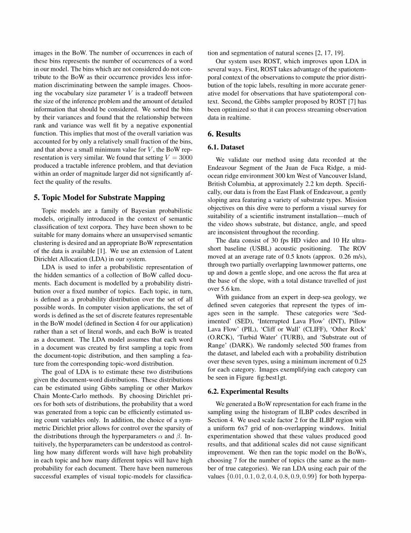
With guidance from an expert in deep-sea geology, wedefined seven categories that represent the types of im-ages seen in the sample. These categories were ‘Sed-imented’ (SED), ‘Interrupted Lava Flow’ (INT), PillowLava Flow’ (PIL), ‘Cliff or Wall’ (CLIFF), ‘Other Rock’(O.RCK), ‘Turbid Water’ (TURB), and ‘Substrate out ofRange’ (DARK). We randomly selected 500 frames fromthe dataset, and labeled each with a probability distributionover these seven types, using a minimum increment of 0.25for each category. Images exemplifying each category canbe seen in Figure fig:best1gt.

6.2. Experimental Results

We generated a BoW representation for each frame in thesampling using the histogram of ILBP codes described inSection 4. We used scale factor 2 for the ILBP region witha uniform 6x7 grid of non-overlapping windows. Initialexperimentation showed that these values produced goodresults, and that additional scales did not cause significantimprovement. We then ran the topic model on the BoWs,choosing 7 for the number of topics (the same as the num-ber of true categories). We ran LDA using each pair of thevalues {0.01, 0.1, 0.2, 0.4, 0.8, 0.9, 0.99} for both hyperpa-

SED

INT

PIL

CLIFF

O.RCK

TURB

DARK

ROCK

NONE

SED

(a) (b)

Figure 3: (a) Representative examples of the categories (top to bottom) ‘Sedimented’, ‘Interrupted Lava Flow’ ‘Pillow LavaFlow’, ‘Cliff or Wall’, ‘Other Rock’, ‘Turbid Water’, and ‘Substrate out of Range’. (b) Images with highest proportion ofwords assigned to each topic. The rows contain the best 7 images for the topics paired with the corresponding category in (a)

(a) (b)

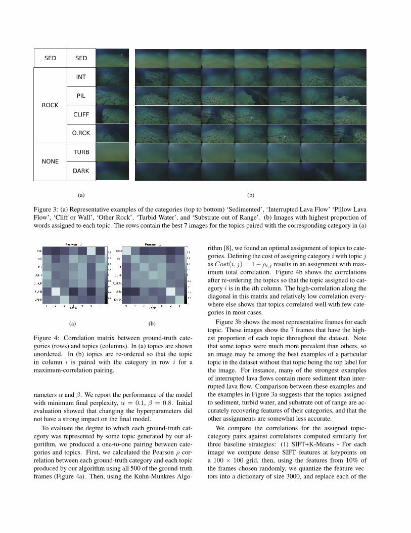
Figure 4: Correlation matrix between ground-truth cate-gories (rows) and topics (columns). In (a) topics are shownunordered. In (b) topics are re-ordered so that the topicin column i is paired with the category in row i for amaximum-correlation pairing.

rameters α and β. We report the performance of the modelwith minimum final perplexity, α = 0.1, β = 0.8. Initialevaluation showed that changing the hyperparameters didnot have a strong impact on the final model.

To evaluate the degree to which each ground-truth cat-egory was represented by some topic generated by our al-gorithm, we produced a one-to-one pairing between cate-gories and topics. First, we calculated the Pearson ρ cor-relation between each ground-truth category and each topicproduced by our algorithm using all 500 of the ground-truthframes (Figure 4a). Then, using the Kuhn-Munkres Algo-

rithm [8], we found an optimal assignment of topics to cate-gories. Defining the cost of assigning category iwith topic jas Cost(i, j) = 1− ρi,j results in an assignment with max-imum total correlation. Figure 4b shows the correlationsafter re-ordering the topics so that the topic assigned to cat-egory i is in the ith column. The high-correlation along thediagonal in this matrix and relatively low correlation every-where else shows that topics correlated well with few cate-gories in most cases.

Figure 3b shows the most representative frames for eachtopic. These images show the 7 frames that have the high-est proportion of each topic throughout the dataset. Notethat some topics were much more prevalent than others, soan image may be among the best examples of a particulartopic in the dataset without that topic being the top label forthe image. For instance, many of the strongest examplesof interrupted lava flows contain more sediment than inter-rupted lava flow. Comparison between these examples andthe examples in Figure 3a suggests that the topics assignedto sediment, turbid water, and substrate out of range are ac-curately recovering features of their categories, and that theother assignments are somewhat less accurate.

We compare the correlations for the assigned topic-category pairs against correlations computed similarly forthree baseline strategies: (1) SIFT+K-Means - For eachimage we compute dense SIFT features at keypoints ona 100 × 100 grid, then, using the features from 10% ofthe frames chosen randomly, we quantize the feature vec-tors into a dictionary of size 3000, and replace each of the

Sediment Interrupted Pillow Cliff Other Rock Turbid Water Out of RangeSIFT+K-Means 0.2898 0.0718 0.4162 0.1721 -0.0137 -0.0271 0.3630LBP+K-Means 0.3526 0.0092 -0.0029 0.3474 0.0508 0.6385 0.4971

LBP+Filt+Discr.+K-Means 0.3661 0.1116 0.0849 0.2916 -0.0685 0.7509 0.3466LBP+Filt+Discr.+Topic-Model 0.7489 0.3899 0.3884 0.4152 0.2580 0.8153 0.5664

(a) Pearson ρ (498) for best-match topic with each category. For LBP+Filt+Discr.+Topic-Model p-value was � 0.001.Sediment Rock No Substrate

SIFT+K-Means 0.4413 0.3492 0.0459LBP+K-Means 0.5059 0.3541 0.5770

LBP+Filt+Discr.+K-Means 0.5350 0.4930 0.4601LBP+Filt+Discr.+Topic-Model 0.7489 0.7156 0.8015

(b) Pearson ρ (498) for best-match topic with each high-level category. For LBP+Filt+Discr.+Topic-Model p-value was � 0.001.

Table 2

original feature vectors with its closest neighbor in the dic-tionary. We compute the histogram of quantized featuresfor each frame, and cluster the feature histograms using K-Means again. (2) LBP+K-Means - We compute ILBP fea-ture histograms for each frame, using mlhspyr lbp withoutthe noise reduction steps described in Sections 4.2.2 and4.3. We cluster the ILBP histograms for each frame usingK-Means. (3) LBP+Filt+Discr.+K-Means We compute thedocument histograms used as input to our topic model, us-ing all steps described above including noise suppressionand selecting only the discriminative histogram bins, butcluster them with K-Means rather than ROST. For each ofthese three strategies, we compute the correlation of eachcluster with each category from the ground-truth, and pro-duce an optimal assignment.

Table 2 shows the values of the correlation for eachtopic-category assignment. This table shows the degreeto which the value of each category was correlated to thevalue of its assigned topic for all of the ground-truth frames.Strong correlation for a category-topic pair suggests that thevalue of the topic was proportional to the value of the cate-gory in most frames. This analysis reflects the quality of themixtures produced by our system rather than just the qualityof the single top category in each frame.

Our method outperformed the three baseline methods,having the highest correlation on 6 out of 7 categories.SIFT+K-Means produced a cluster with high correlationwith the pillow category, but its performance on all othercategories was poor. These values show a median strengthof association 2.5 times larger between topics and cate-gories than beteen SIFT clusters and categories (strength ofassociation is defined as the absolute value of correlation).

Note that for our topic-model approach, p-values were� 0.001, whereas for the other approaches, p-values var-ied, sometimes taking significantly higher values. Thesep-values represent a strong rejection of the hypothesis that

the topics were not correlated with the categories for ourmethod, and a weaker one for the baseline strategies.

In absolute terms, the values of the correlations reflectthe intuition given by the best examples of each topic: Thecategories sediment, turbid water, and no substrate are eachstrongly correlated with their assigned topic, but the othercategories are only weakly correlated with their assign-ment. Therefore, we additionally analyze our system’s per-formance classifying the high-level categories ‘Sediment’,‘Rocky’, and ‘No Substrate’. These categories were con-structed by combining the original categories, as seen in theleftmost column of Figure 3a. We combined the ground-truth labels, topics, and labels for the three baseline meth-ods by summing over the groups to be combined into eachof the three categories. The performance of the resultingmodels is presented in Table 2b, showing that our methodhas strong correlations between the combined topics and allthree of the high-level categories.

7. DiscussionOur results constitute a preliminary success in unsu-

pervised substrate type mapping on a challenging videodataset. The categories not consistently identified by oursystem were semantically overlapping, and to some degreevisually similar. This has allowed us to make use of the sys-tem as-is to map higher-level substrate categories. Althoughless specific than the original categories, this still representsinteresting and useful data to ocean scientists. We presenta map of these substrate types in Figure 5. Maps of thistype provide an interface between our method and biolog-ical or geological research which seeks to use informationabout substrate type. For instance, this map could be used inconjunction with a map of observations of a certain speciesto help answer questions about how habitat suitability is re-lated to substrate type. Note that the substrate type mixturesare spatially consistent and vary smoothly in adjacent sam-

Figure 5: ROV track with topic mixtures at each sample point. The line represents the path of the ROV, and each point is thelocation of a substrate sample image. At each point, there are circles for each of the three topics, with their sizes representingthe mixture of the topics in that sample.

ples. This reflects the transitional areas which are not welldescribed by a single label.

In collecting the ground-truth data, we observed that acorrect classification is extremely context dependent andsomewhat subjective. Depending on the intended applica-tion, the salience of different features varies subjectively,for example, a frame containing mainly sediment with onearea of exposed pillow lava might might be of high interestto one researcher but of little interest to another. In addition,it is unclear how a ground-truth dataset should measure theamount a substrate type is represented in each frame. Al-though it is tempting to use percent cover as a way to quan-tify these observations, this approach depends on havingvery precise definitions of the boundaries between substratetypes which are not always available.

Emerging methods for hierarchical topic models couldhelp to resolve the differences in scale of similarity betweenthe desired categories [3]. In addition, directly incorporat-ing the noise reduction and vocabulary learning steps intothe probabilistic model could improve results by estimatingthe parameters from data, rather than setting them based onmanual experimentation.

As a preliminary investigation for future work, we ranour algorithm on two additional datasets: One on the nearbyHigh-Rise vent structure featuring a completely different setof substrate types and geoforms, and a second from Barkley

Canyon—a biological diverse yet geologically uniform en-vironment composed mainly of sediment. Preliminary re-sults appear promising, suggesting that this system couldbe used in other environments with minimal modifications.

8. Conclusion

We have presented a method for learning and mappingdeep-sea substrate types. This method computes a mixtureof types for each frame in an ROV video using a texture-based BoW representation of the images and a spatiotem-poral topic model. It requires minimal training data, andincludes measures to compensate for the different kindsof noise associated with deep-sea ROV video recordings.We have shown that in a mid-ocean ridge flank environ-ment, this method recovers topics that correlate highly withground-truth substrate categories. Our analysis shows thatthe described pipeline significantly outperforms conven-tional methods, demonstrating the utility of the combinationof proposed techniques for the substrate labelling task.

9. Acknowledgement

The authors thank Steven F. Mihaly, Fabio C. De Leo,Marlene A. Jeffries and Laurence A. Coogan for their sug-gestions and contributions to this work.

References[1] D. M. Blei. Probabilistic topic models. Commun. ACM,

55(4):77–84, Apr. 2012.[2] L. Cao and L. Fei-Fei. Spatial coherent latent topic model

for concurrent object segmentation and classification. Inter-national Conference on Computer Vision, 2007.

[3] F. Chamroukhi, M. Bartcus, and H. Glotin. Bayesian non-parametric parsimonious gaussian mixture for clustering. InIn Proc. of Int. Conf. on Pattern Recognition (ICPR), IEEE,Stockholm, 2014.

[4] Y. Girdhar. Unsupervised Semantic Perception, Summariza-tion, and Autonomous Exploration for Robots in Unstruc-tured Environments. PhD thesis, McGill University, 2014.

[5] Y. Girdhar and G. Dudek. Modeling curiosity in a mobilerobot for long-term autonomous exploration and monitoring.Autonomous Robots, pages 1–12, 2015.

[6] Y. A. Girdhar, W. Cho, M. Campbell, J. Pineda, E. Clarke,and H. Singh. Anomaly detection in unstructured environ-ments using bayesian nonparametric scene modeling. CoRR,abs/1509.07979, 2015.

[7] Y. A. Girdhar and G. Dudek. Gibbs sampling strategiesfor semantic perception of streaming video data. CoRR,abs/1509.03242, 2015.

[8] H. W. Kuhn. The hungarian method for the assignmentproblem. Naval Research Logistics Quarterly, 2(1-2):83–97,1955.

[9] M. Lacharite, A. Metaxas, and P. Lawton. Using object-based image analysis to determine seafloor fine-scale fea-tures and complexity. Limnology and Oceanography: Meth-ods, 13(10):553–567, 2015.

[10] S. Liao, X. Zhu, Z. Lei, L. Zhang, and S. Li. Learning multi-scale block local binary patterns for face recognition. Ad-vances in Biometrics, pages 828–837, 2007.

[11] MATLAB. Version 8.6.0 (R2015b). The MathWorks Inc.,Natick, Massachusetts, 2015.

[12] A. Oliva and A. Torralba. Modeling the shape of the scene: Aholistic representation of the spatial envelope. InternationalJournal of Computer Vision, 42(3):145–175, 2001.

[13] S. Paris, X. Halkias, and H. Glotin. Efficient Bag ofScenes Analysis for Image Categorization. InternationalConference on Pattern Recognition Applications and Meth-ods, 2012.

[14] O. Pizarro, P. Rigby, M. Johnson-Roberson, S. B. Williams,and J. Colquhoun. Towards image-based marine habitat clas-sification. Oceans 2008, pages 1–7, 2008.

[15] O. Pizarro, S. Williams, and J. Colquhoun. Topic-based habi-tat classification using visual data. In OCEANS 2009 - EU-ROPE, pages 1–8, May 2009.

[16] T. Schoening, T. Kuhn, and T. Nattkemper. Seabed clas-sification using a bag-of-prototypes feature representation.In Computer Vision for Analysis of Underwater Imagery(CVAUI), 2014 ICPR Workshop on, pages 17–24, Aug 2014.

[17] C. Wang, D. Blei, and L. Fei-Fei. Simultaneous image clas-sification and annotation. 2009 IEEE Computer Society Con-ference on Computer Vision and Pattern Recognition Work-shops, CVPR Workshops 2009, pages 1903–1910, 2009.

[18] S. B. Williams, O. Pizarro, J. M. Webster, R. J. Beaman,I. Mahon, M. Johnson-Roberson, and T. C. L. Bridge. Au-tonomous underwater vehicle-assisted surveying of drownedreefs on the shelf edge of the Great Barrier Reef, Australia.Journal of Field Robotics, 27(5):675–697, Aug. 2010.

[19] B. Zhao, L. Fei-Fei, and E. Xing. Image segmentationwith topic random field. In K. Daniilidis, P. Maragos, andN. Paragios, editors, Computer Vision - ECCV 2010, volume6315 of Lecture Notes in Computer Science, pages 785–798.Springer Berlin Heidelberg, 2010.