Learning Application Models for Utility

Resource Planning Piyush Shivam, Shivnath Babu, Jeff Chase

Duke University

IEEE International Conference on Autonomic Computing (ICAC), June 2006

C3

C1

C2

Site A

Site B

Site C

Task scheduler

Task workflow

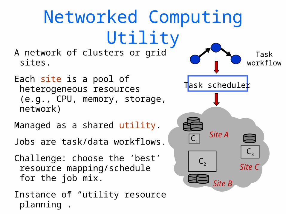
A network of clusters or grid sites.

Each site is a pool of heterogeneous resources (e.g., CPU, memory, storage, network)

Managed as a shared utility.

Jobs are task/data workflows.

Challenge: choose the ‘best’ resource mapping/schedule for the job mix.

Instance of “utility resource planning”.

Solution under construction: NIMO

Networked Computing Utility

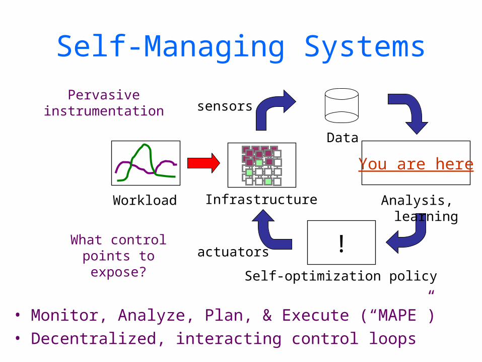
Self-Managing Systems

• Monitor, Analyze, Plan, & Execute (“MAPE”)• Decentralized, interacting control loops

Workload

Data

Analysis, learning

Self-optimization policy

Infrastructure

You are here

!

sensors

actuators

Pervasive instrumentation

What control points to expose?

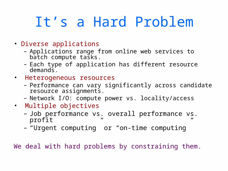
It’s a Hard Problem• Diverse applications

– Applications range from online web services to batch compute tasks.

– Each type of application has different resource demands.

• Heterogeneous resources– Performance can vary significantly across candidate

resource assignments.– Network I/O: compute power vs. locality/access

• Multiple objectives– Job performance vs. overall performance vs. profit– “Urgent computing” or “on-time computing”

We deal with hard problems by constraining them.

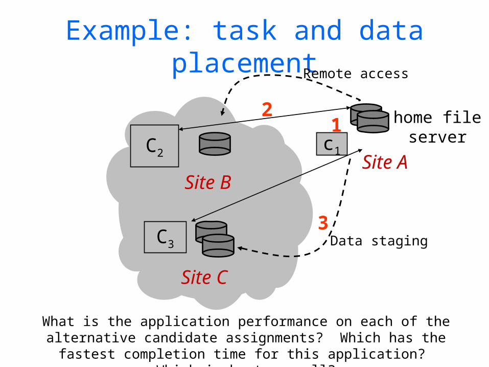
Example: task and data placement

1C2

c1Site A

Site B

C3

Site C

home file server

2

What is the application performance on each of the alternative candidate assignments? Which has the fastest completion time for this application? Which is best overall?

Remote access

3Data staging

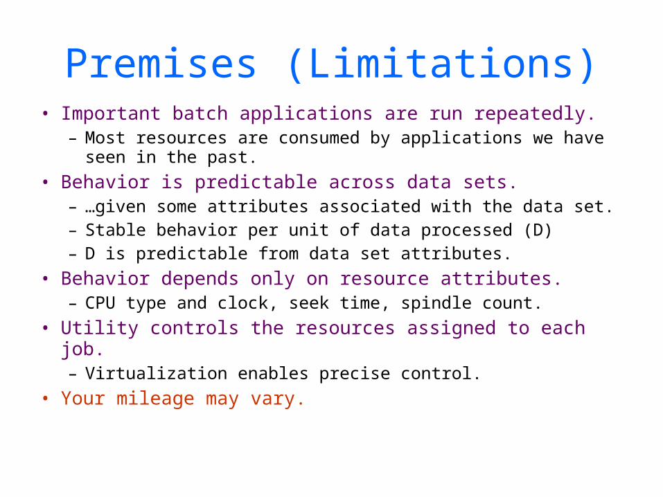
Premises (Limitations)• Important batch applications are run repeatedly.

– Most resources are consumed by applications we have seen in the past.

• Behavior is predictable across data sets.– …given some attributes associated with the data set.– Stable behavior per unit of data processed (D)– D is predictable from data set attributes.

• Behavior depends only on resource attributes.– CPU type and clock, seek time, spindle count.

• Utility controls the resources assigned to each job.– Virtualization enables precise control.

• Your mileage may vary.

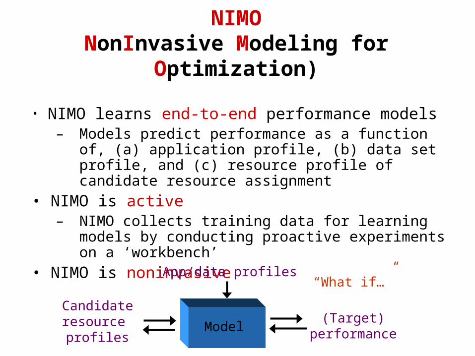
NIMONonInvasive Modeling for

Optimization)

• NIMO learns end-to-end performance models– Models predict performance as a function of, (a)

application profile, (b) data set profile, and (c) resource profile of candidate resource assignment

• NIMO is active– NIMO collects training data for learning models by

conducting proactive experiments on a ‘workbench’• NIMO is noninvasive

App/data profiles

(Target) performance

Candidate resource profiles

Model

“What if…”

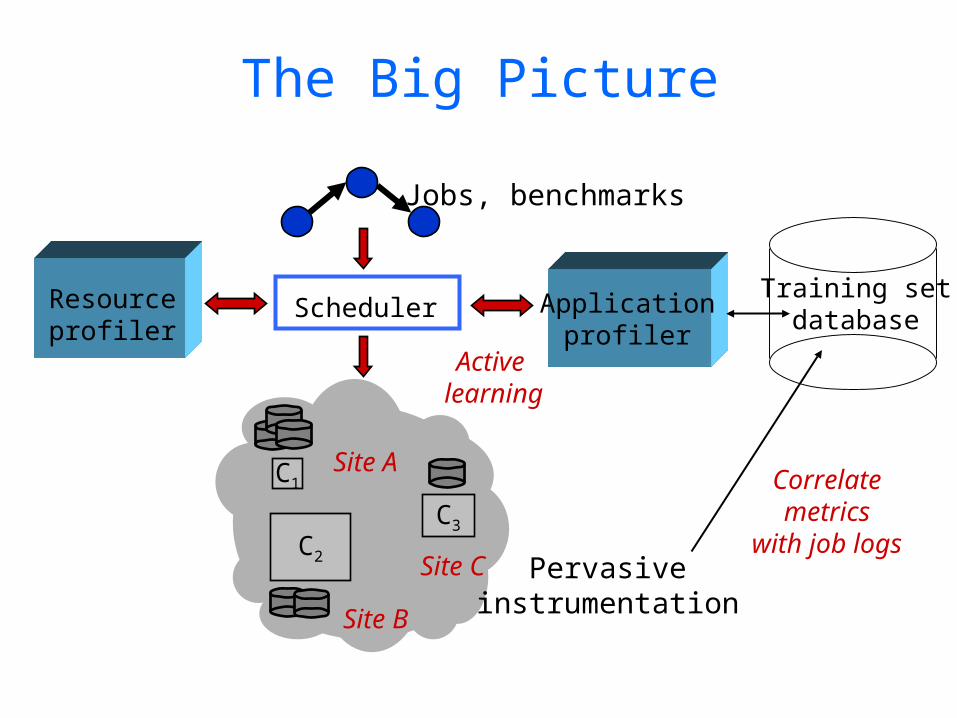
Applicationprofiler

Training setdatabase

Active learning

C3

C1

C2

Site A

Site B

Site C

SchedulerResourceprofiler

The Big Picture

Jobs, benchmarks

Pervasive instrumentation

Correlate metrics

with job logs

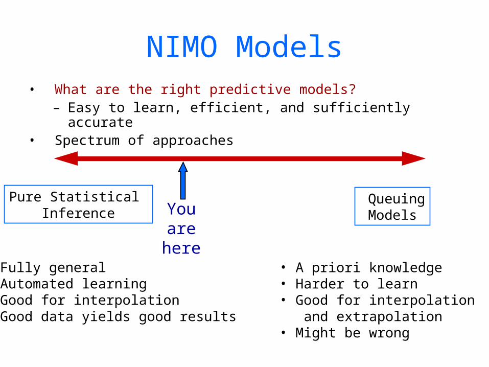
Pure Statistical Inference

QueuingModels

• Fully general• Automated learning• Good for interpolation• Good data yields good results

• A priori knowledge• Harder to learn• Good for interpolation and extrapolation• Might be wrong

You are here

• What are the right predictive models?– Easy to learn, efficient, and sufficiently accurate

• Spectrum of approaches

NIMO Models

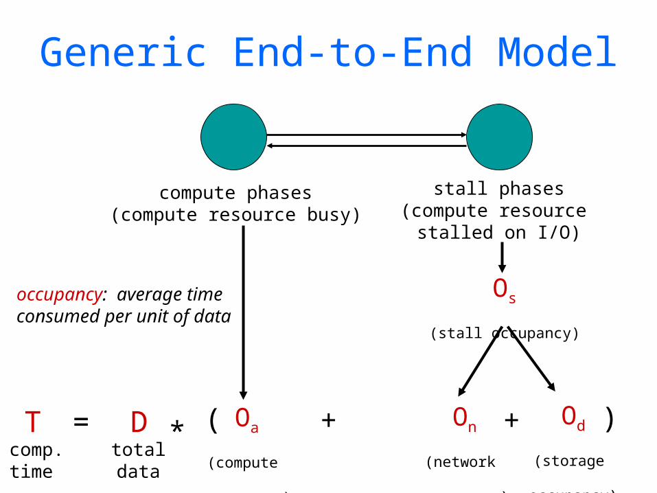
Generic End-to-End Model

compute phases(compute resource busy)

stall phases(compute resource

stalled on I/O)

Od

(storage

occupancy)

On

(network

occupancy)

+ + )(T = D *totaldata

comp.time

Oa

(compute

occupancy)

Os

(stall occupancy)

occupancy: average time consumed per unit of data

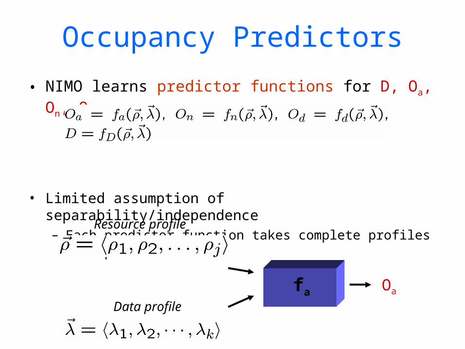
Occupancy Predictors

• NIMO learns predictor functions for D, Oa, On, Od

• Limited assumption of separability/independence– Each predictor function takes complete profiles as

inputs.Resource profile

Data profile

Oa fa

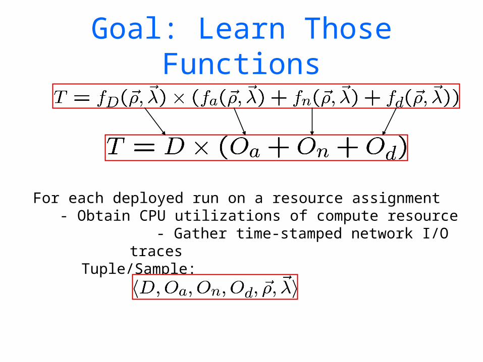
Goal: Learn Those Functions

For each deployed run on a resource assignment - Obtain CPU utilizations of compute resource

- Gather time-stamped network I/O traces Tuple/Sample:

Independent variables

Dependent variables

Resource profile ( )

Dataprofile ( )

Statistical Learning

Complexity (e.g., latency hiding, concurrency, arm contention) is captured implicitly in the training data rather than in the structure of the model.

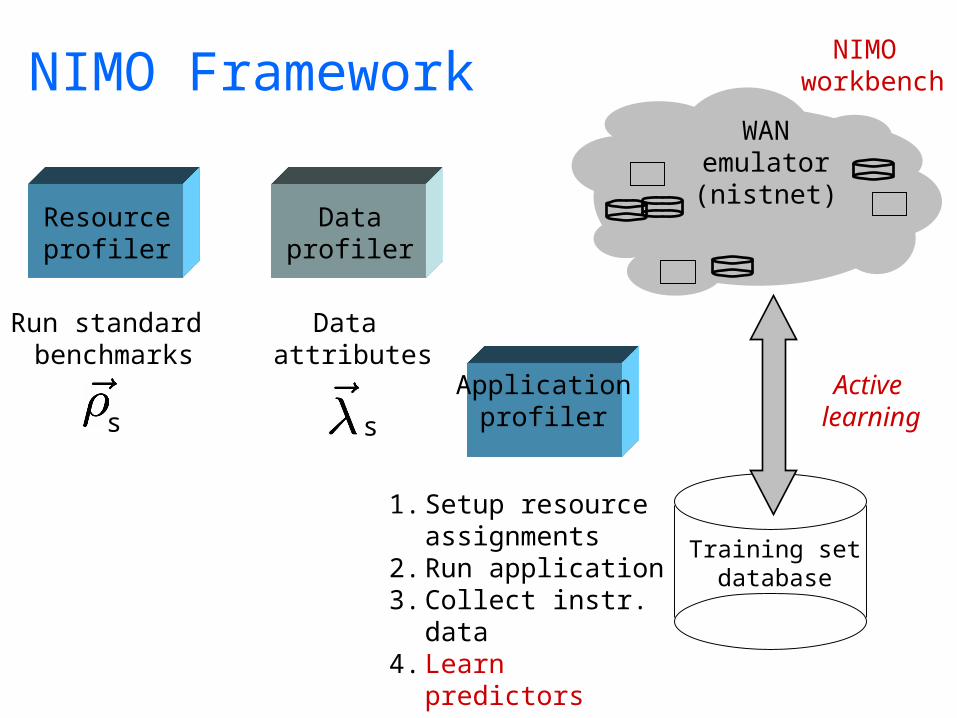
NIMO Framework

Applicationprofiler

Resourceprofiler

Dataprofiler

WANemulator(nistnet)

NIMO workbench

Run standard benchmarks

1. Setup resource assignments

2. Run application3. Collect instr. data4. Learn predictors

Training setdatabase

Active learning

Data attributes

s s

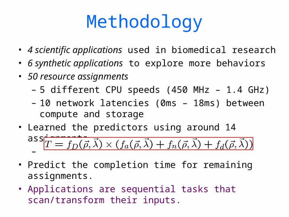
Methodology• 4 scientific applications used in biomedical research• 6 synthetic applications to explore more behaviors• 50 resource assignments

– 5 different CPU speeds (450 MHz – 1.4 GHz)– 10 network latencies (0ms – 18ms) between

compute and storage• Learned the predictors using around 14

assignments–

• Predict the completion time for remaining assignments.

• Applications are sequential tasks that scan/transform their inputs.

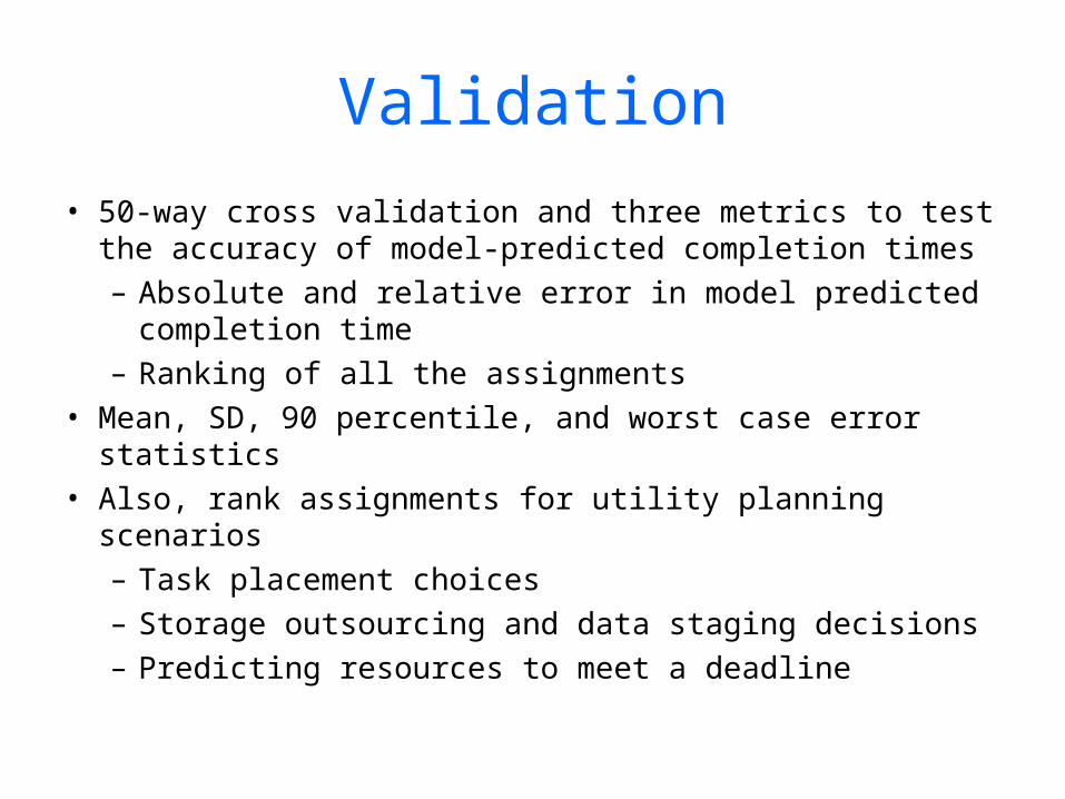
Validation

• 50-way cross validation and three metrics to test the accuracy of model-predicted completion times – Absolute and relative error in model predicted

completion time – Ranking of all the assignments

• Mean, SD, 90 percentile, and worst case error statistics

• Also, rank assignments for utility planning scenarios– Task placement choices – Storage outsourcing and data staging decisions– Predicting resources to meet a deadline

Results Summary

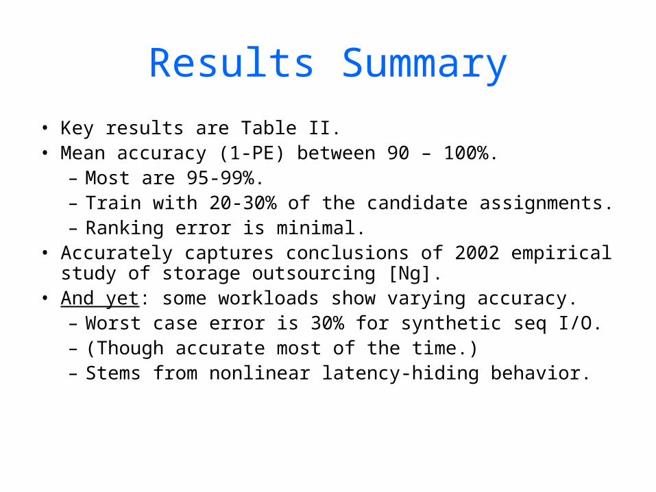
• Key results are Table II.• Mean accuracy (1-PE) between 90 – 100%.

– Most are 95-99%.– Train with 20-30% of the candidate

assignments.– Ranking error is minimal.

• Accurately captures conclusions of 2002 empirical study of storage outsourcing [Ng].

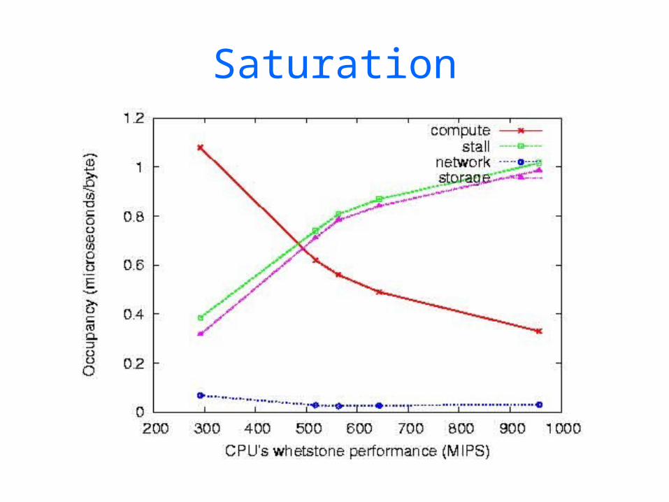
• And yet: some workloads show varying accuracy.– Worst case error is 30% for synthetic seq I/O.– (Though accurate most of the time.)– Stems from nonlinear latency-hiding behavior.

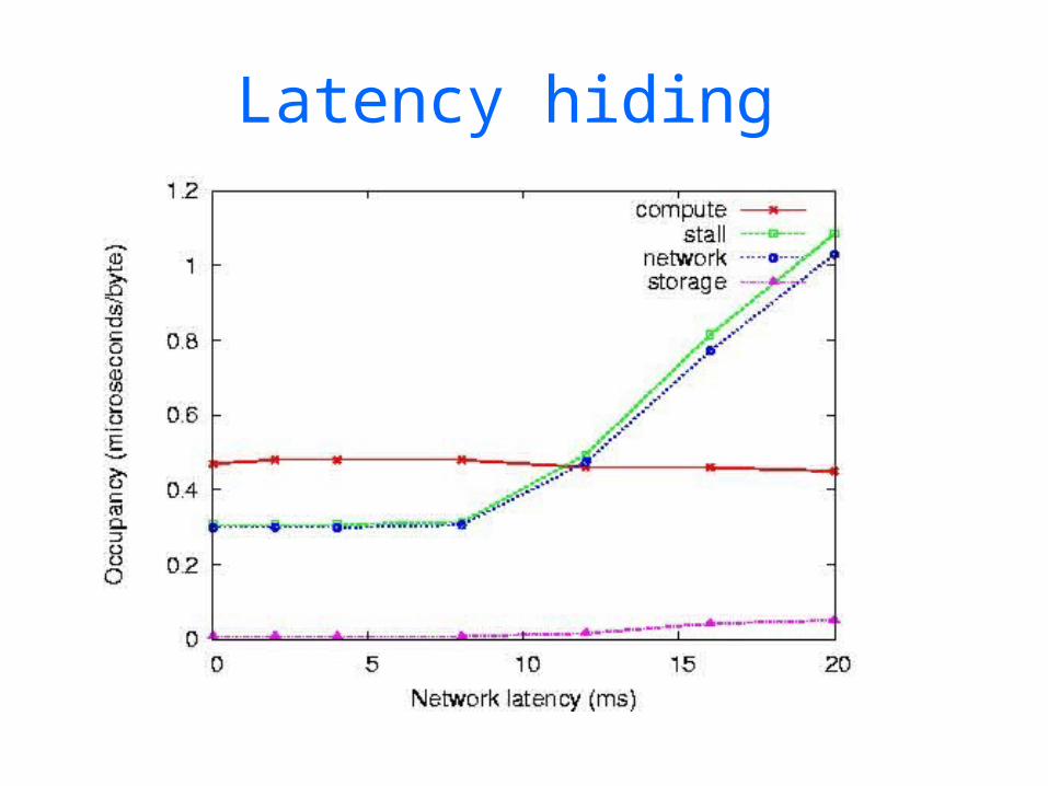
Latency hiding

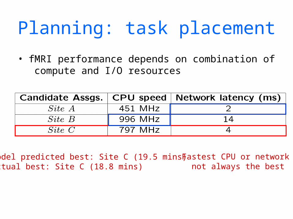
Planning: task placement

• fMRI performance depends on combination of compute and I/O resources

Model predicted best: Site C (19.5 mins)Actual best: Site C (18.8 mins)

Fastest CPU or network not always the best

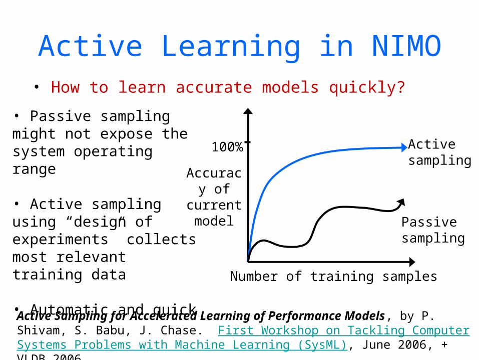
Active Learning in NIMO

Passive sampling

Active sampling

Number of training samples

Accuracy of

current model

100%

• Passive sampling might not expose the system operating range

• Active sampling using “design of experiments” collects most relevant training data

• Automatic and quick

• How to learn accurate models quickly?

Active Sampling for Accelerated Learning of Performance Models, by P. Shivam, S. Babu, J. Chase. First Workshop on Tackling Computer Systems Problems with Machine Learning (SysML), June 2006, + VLDB 2006

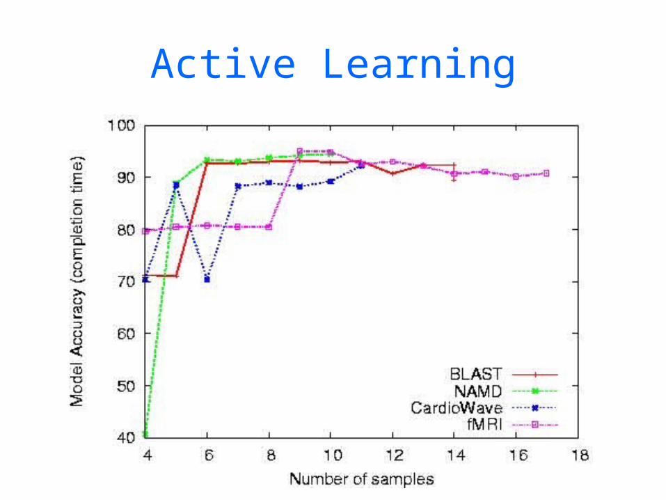
Active Learning

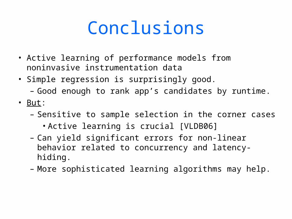
Conclusions

• Active learning of performance models from noninvasive instrumentation data

• Simple regression is surprisingly good.– Good enough to rank app’s candidates by runtime.

• But:– Sensitive to sample selection in the corner cases

• Active learning is crucial [VLDB06]– Can yield significant errors for non-linear behavior

related to concurrency and latency-hiding.– More sophisticated learning algorithms may help.

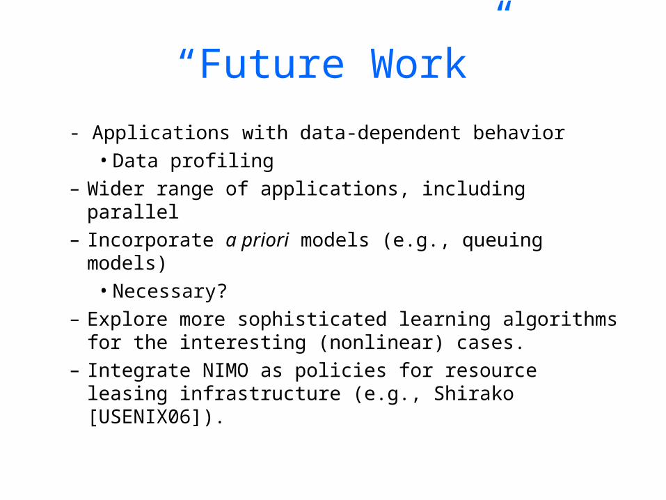
“Future Work”

- Applications with data-dependent behavior• Data profiling

– Wider range of applications, including parallel– Incorporate a priori models (e.g., queuing

models)• Necessary?

– Explore more sophisticated learning algorithms for the interesting (nonlinear) cases.

– Integrate NIMO as policies for resource leasing infrastructure (e.g., Shirako [USENIX06]).

http://www.cs.duke.edu/~chasehttp://www.cs.duke.edu/~chase

Saturation

We have data

I’m sure the information is here…SomewhereSomewhere..

Redundant

irrelevant

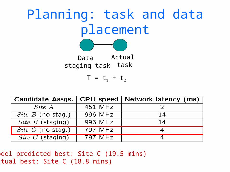
Data staging task

Actual task

T = t1 + t2

Planning: task and data placement

Model predicted best: Site C (19.5 mins)Actual best: Site C (18.8 mins)

Experimental Evaluation• Applied NIMO to do accurate resource planning

– Several real and synthetic batch applications – Heterogeneous compute and network resources

• Planning Scenarios– Task placement choices – Storage outsourcing and data staging decisions– Predicting resources that meet a target performance

• NIMO learned accurate models using only 10-25% of the total training samples

Future Directions

• Integrate NIMO within an on-demand resource brokering architecture, e.g., Cereus [USENIX 2006]

• Investigate the continuum of models• Apply NIMO to a wider variety of applications and

resources

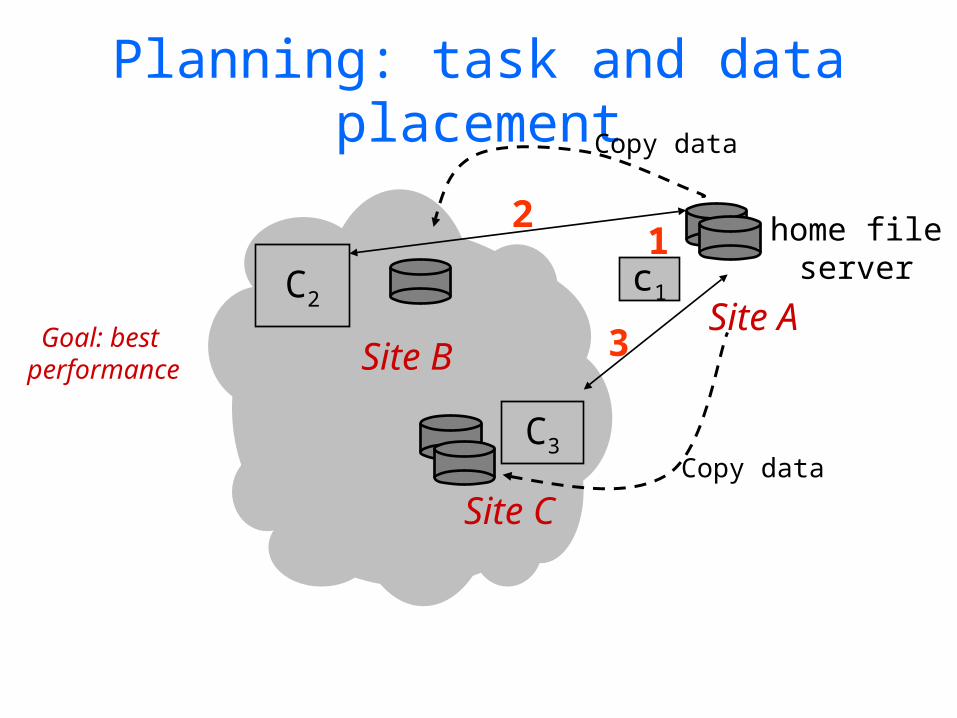
Planning: task and data placement

1C2

c1Site A

Site B

C3

Site C

home file server

2

Goal: best performance

3

Copy data

Copy data

Other Scenarios

• Viability of storage outsourcing• Candidates that meet a target completion time• Details in ICAC 2006

C3C1

C2

Site A

Site B

Site C

home file server

P1

P2P3

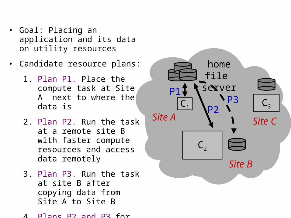
• Goal: Placing an application and its data on utility resources

• Candidate resource plans:

1. Plan P1. Place the compute task at Site A next to where the data is

2. Plan P2. Run the task at a remote site B with faster compute resources and access data remotely

3. Plan P3. Run the task at site B after copying data from Site A to Site B

4. Plans P2 and P3 for Site C

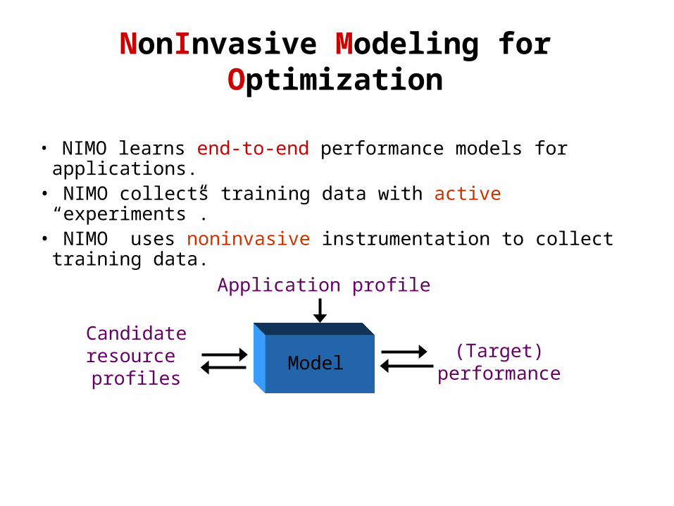
NonInvasive Modeling for Optimization

• NIMO learns end-to-end performance models for applications.• NIMO collects training data with active “experiments”.• NIMO uses noninvasive instrumentation to collect training

data.

Application profile

(Target) performance

Candidate resource profiles

Model

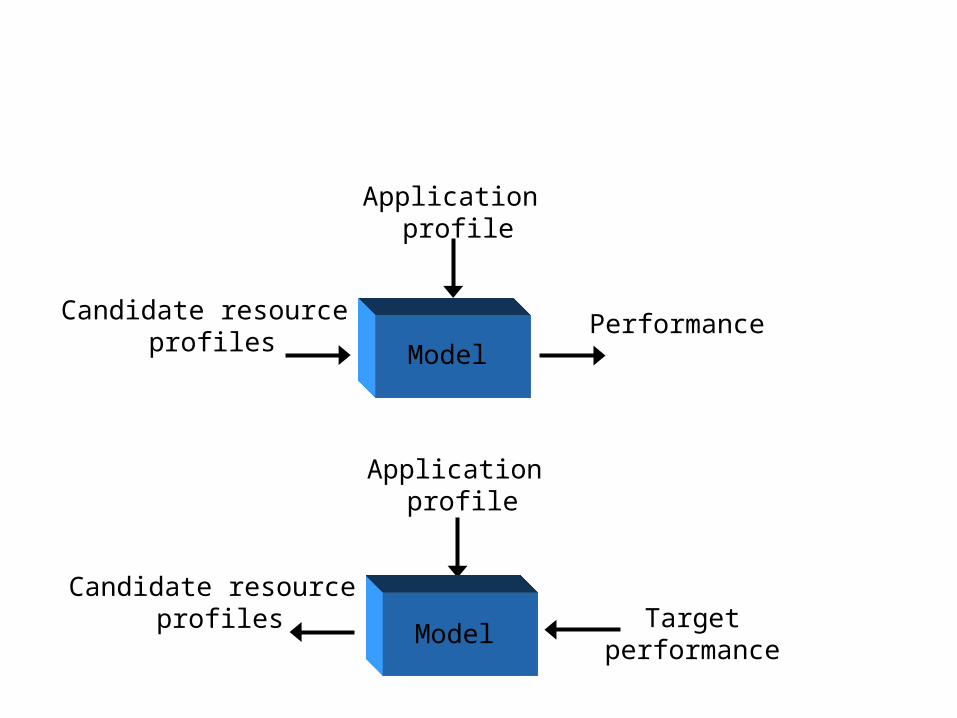
Application profile

PerformanceCandidate resource profiles Model

Candidate resource profiles

Application profile

Targetperformance

Model

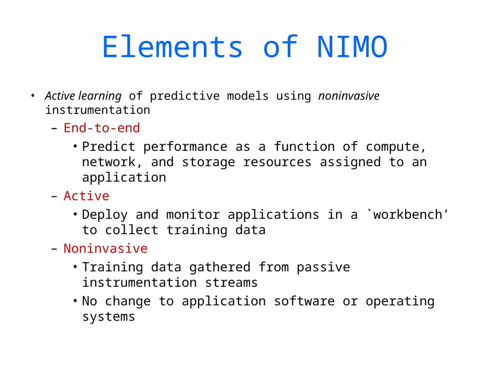
Elements of NIMO• Active learning of predictive models using noninvasive

instrumentation

– End-to-end• Predict performance as a function of compute, network,

and storage resources assigned to an application– Active

• Deploy and monitor applications in a `workbench’ to collect training data

– Noninvasive• Training data gathered from passive instrumentation

streams• No change to application software or operating systems

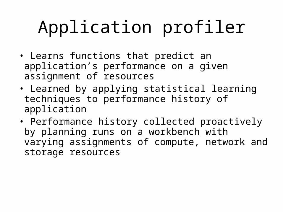
Application profiler

• Learns functions that predict an application’s performance on a given assignment of resources

• Learned by applying statistical learning techniques to performance history of application

• Performance history collected proactively by planning runs on a workbench with varying assignments of compute, network and storage resources

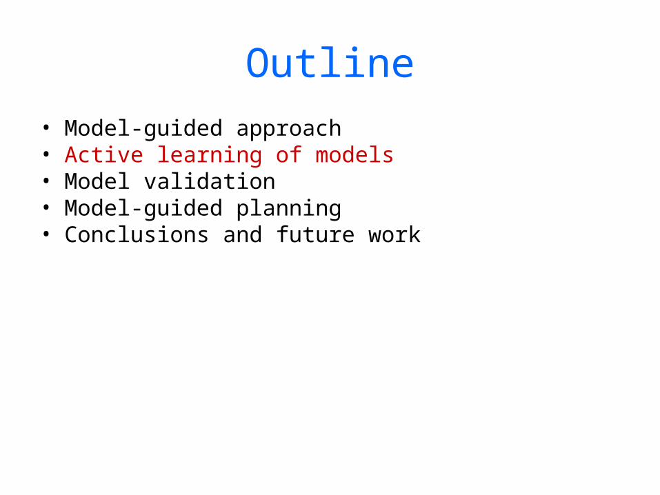
Outline• Model-guided approach • Active learning of models • Model validation • Model-guided planning• Conclusions and future work

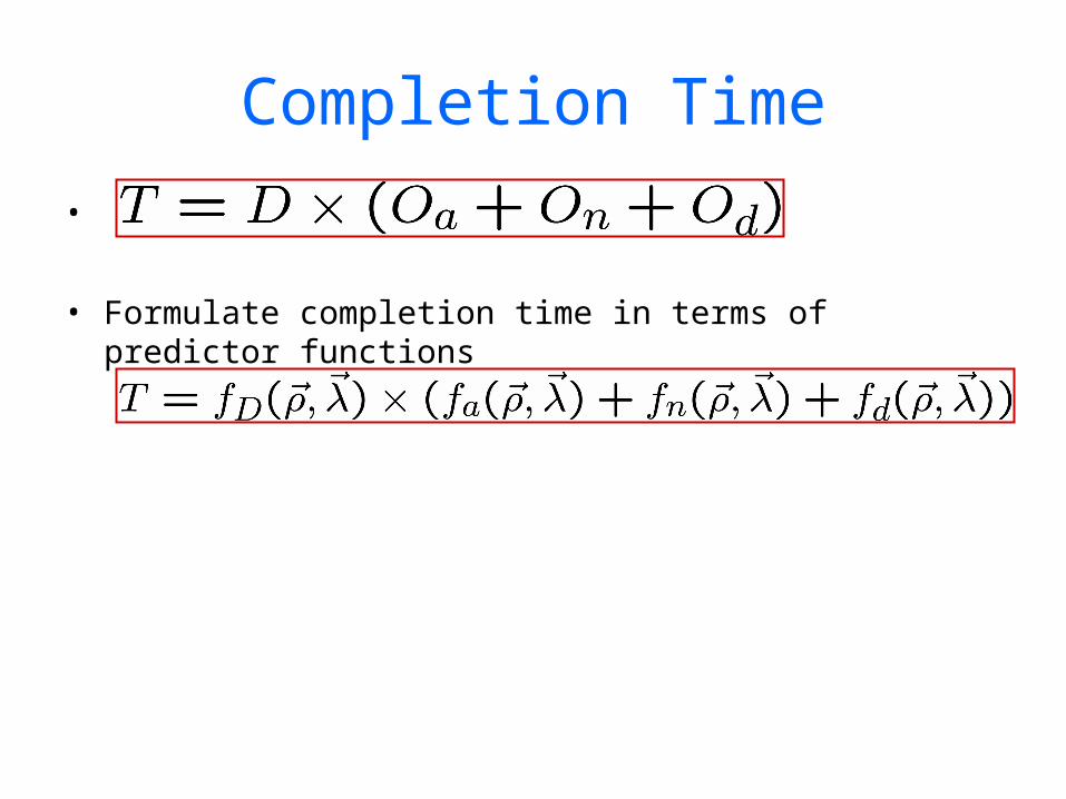
Completion Time

•

• Formulate completion time in terms of predictor functions

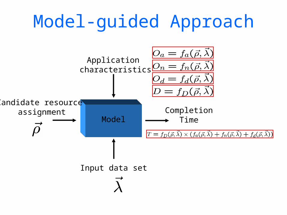
Model-guided Approach

Application characteristics

Completion Time

Candidate resource assignment

Model

Input data set

Active and Noninvasive

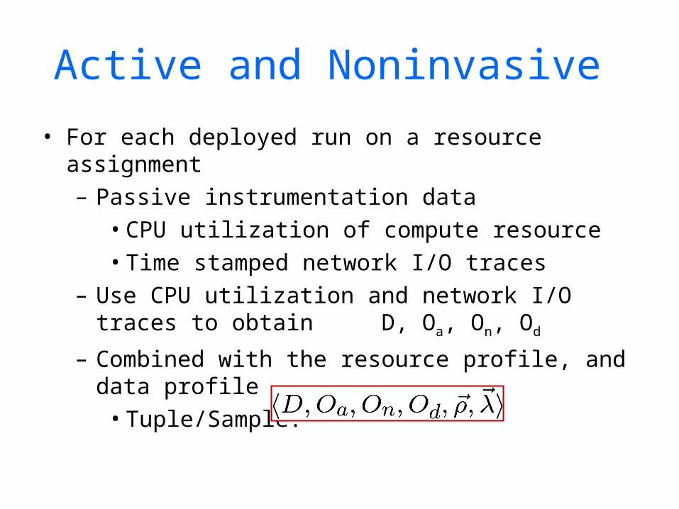
• For each deployed run on a resource assignment – Passive instrumentation data

• CPU utilization of compute resource • Time stamped network I/O traces

– Use CPU utilization and network I/O traces to obtain D, Oa, On, Od

– Combined with the resource profile, and data profile• Tuple/Sample:

Capturing complexity

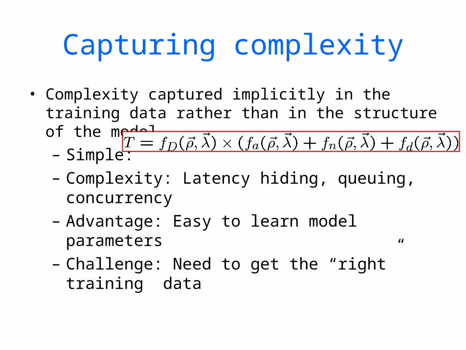
• Complexity captured implicitly in the training data rather than in the structure of the model– Simple: – Complexity: Latency hiding, queuing,

concurrency– Advantage: Easy to learn model parameters– Challenge: Need to get the “right” training

data

Active Learning

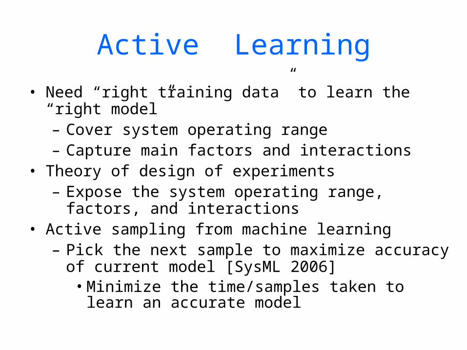
• Need “right training data” to learn the “right model”– Cover system operating range– Capture main factors and interactions

• Theory of design of experiments– Expose the system operating range, factors, and

interactions• Active sampling from machine learning

– Pick the next sample to maximize accuracy of current model [SysML 2006]• Minimize the time/samples taken to learn an

accurate model

Outline• Model-guided approach • Active learning of models • Model validation • Model-guided planning • Conclusions and future work

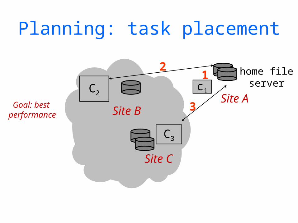
Planning: task placement

1C2

c1Site A

Site B

C3

Site C

home file server

2

Goal: best performance

3

Summary

• Holistic view of network and edge resources for networked application services.– NSF GENI initiative (http://www.geni.net)

• “Autonomic” management– Sense and respond– Optimizing control loops based on learned

models• Large-scale systems involve a factoring of control

functions and policies across multiple actors.– Emergent behavior– Incentives and secure, accountable control