Learning Acyclic Probabilistic Circuits Using Test Paths · Learning Acyclic Probabilistic Circuits...
33
Journal of Machine Learning Research ?? (2009) ???–??? Submitted 1/09; Revised 6/09; Published ?/?? Learning Acyclic Probabilistic Circuits Using Test Paths Dana Angluin [email protected] James Aspnes [email protected] Department of Computer Science Yale University Jiang Chen [email protected] Yahoo! Inc. 701 First Avenue Sunnyvale, CA 94086 David Eisenstat [email protected] Lev Reyzin [email protected] Department of Computer Science Yale University Editor: Rocco Servedio Abstract We define a model of learning probabilistic acyclic circuits using value injection queries, in which fixed values are assigned to an arbitrary subset of the wires and the value on the single output wire is observed. We adapt the approach of using test paths from the Circuit Builder algorithm (Angluin et al., 2009) to show that there is a polynomial time algorithm that uses value injection queries to learn acyclic Boolean probabilistic circuits of constant fan-in and log depth. We establish upper and lower bounds on the attenuation factor for general and transitively reduced Boolean probabilistic circuits of test paths versus general experiments. We give computational evidence that a polynomial time learning algorithm using general value injection experiments may not do much better than one using test paths. For probabilistic circuits with alphabets of size three or greater, we show that the test path lemmas (Angluin et al., 2009, 2008b) fail utterly. To overcome this obstacle, we introduce function injection queries, in which the values on a wire may be mapped to other values rather than just to themselves or constants, and prove a generalized test path lemma for this case. Keywords: nonadaptive learning algorithms, probabilistic circuits, causal Bayesian net- works, value injection queries, test paths 1. Introduction Probabilistic networks are used as models in a variety of domains, for example, gene interac- tion networks, social networks and causal reasoning. In a binary model of gene interaction, the state of each gene is either active or inactive, and the state of each gene is determined as a function of the states of some number of other genes, its inputs. In a probabilistic c 2009 Dana Angluin and James Aspnes and Jiang Chen and David Eisenstat and Lev Reyzin.
Transcript of Learning Acyclic Probabilistic Circuits Using Test Paths · Learning Acyclic Probabilistic Circuits...
Journal of Machine Learning Research ?? (2009) ???–??? Submitted 1/09; Revised 6/09; Published ?/??
Learning Acyclic Probabilistic Circuits Using Test Paths
Dana Angluin [email protected] Aspnes [email protected] of Computer ScienceYale University
Jiang Chen [email protected]! Inc.701 First AvenueSunnyvale, CA 94086
David Eisenstat [email protected]
Lev Reyzin [email protected]
Department of Computer ScienceYale University
Editor: Rocco Servedio
Abstract
We define a model of learning probabilistic acyclic circuits using value injection queries, inwhich fixed values are assigned to an arbitrary subset of the wires and the value on thesingle output wire is observed. We adapt the approach of using test paths from the CircuitBuilder algorithm (Angluin et al., 2009) to show that there is a polynomial time algorithmthat uses value injection queries to learn acyclic Boolean probabilistic circuits of constantfan-in and log depth. We establish upper and lower bounds on the attenuation factor forgeneral and transitively reduced Boolean probabilistic circuits of test paths versus generalexperiments. We give computational evidence that a polynomial time learning algorithmusing general value injection experiments may not do much better than one using testpaths. For probabilistic circuits with alphabets of size three or greater, we show that thetest path lemmas (Angluin et al., 2009, 2008b) fail utterly. To overcome this obstacle, weintroduce function injection queries, in which the values on a wire may be mapped to othervalues rather than just to themselves or constants, and prove a generalized test path lemmafor this case.
Keywords: nonadaptive learning algorithms, probabilistic circuits, causal Bayesian net-works, value injection queries, test paths
1. Introduction
Probabilistic networks are used as models in a variety of domains, for example, gene interac-tion networks, social networks and causal reasoning. In a binary model of gene interaction,the state of each gene is either active or inactive, and the state of each gene is determinedas a function of the states of some number of other genes, its inputs. In a probabilistic
c©2009 Dana Angluin and James Aspnes and Jiang Chen and David Eisenstat and Lev Reyzin.
Angluin, Aspnes, Chen, Eisenstat and Reyzin
variant of the model, the activation function specifies, for each possible combination of thestates of the inputs, the probability that the gene will be active (Friedman et al., 2000).In the independent cascade model of social networks, the state of each agent is active orinactive and for each pair (u, v) of agents, there is a probability that the activation of u willcause v to become active. Kempe, Kleinberg, and Tardos (2003, 2005) study the problem ofmaximizing influence in this and related models of social networks. In a Bayesian networkthere is an acyclic directed graph and a joint probability distribution over the node valuessuch that the joint distribution is the product of each of the marginal distributions for eachnode given the values of the parents (in-neighbors) of the node.
A fundamental question is how much we can infer about the properties and structureof such networks from observing and experimenting with their behaviors. Prior researchgives evidence from cryptography that there may be no polynomial time algorithm to learnBoolean functions represented by acyclic circuits of constant fan-in and depth O(log n)when we can set only the inputs of the circuit and observe only the output (Angluin andKharitonov, 1995). In this paper we consider a different setting, value injection queries,in which we can fix the values on any subset of wires in the target circuit, but still onlyobserve the output of the circuit.
The concept of value injection queries was inspired by models of gene suppression andgene overexpression in the study of gene interaction networks (Akutsu et al., 2003; Idekeret al., 2000) and was introduced by Angluin et al. (2009). In a causal Bayesian networkthere is an additional action do(X = x) that forces a node X to take on a value x (Pearl,2000). A value injection query may also be viewed as a set of such actions, one for eachwire fixed to a value.
Angluin et al. (2009) investigate the learnability of deterministic circuits using valueinjection queries and behavioral equivalence queries. Polynomial time learning algorithmsusing just value injection queries are given for two classes of acyclic circuits. Circuit Builderuses value injection queries to learn acyclic deterministic circuits with constant-size alpha-bets, constant fan-in and depth O(log n) up to behavioral equivalence in polynomial time.Another algorithm is given that learns constant-depth acyclic Boolean circuits with NOTgates and unbounded fan-in AND, OR, NAND and NOR gates up to behavioral equivalencein polynomial time using value injection queries. Negative results include an exponentiallower bound on the number of value injection queries to learn acyclic Boolean circuits ofunbounded depth and unbounded fan-in, and the NP-hardness of learning acyclic Booleancircuits of unbounded depth and constant fan-in using value injection queries.
In extending these results to analog circuits, Angluin et al. (2008b) consider circuits withpolynomial-size alphabets. They give evidence of the computational hardness of learningacyclic circuits over a polynomial-size alphabet even if the depth is restricted to O(log n),motivating structural restrictions on the graphs of the circuits to achieve polynomial timelearnability. They give the Distinguishing Paths Algorithm, which uses value injectionqueries and learns acyclic deterministic circuits that are transitively reduced and havepolynomial-size alphabets, constant fan-in and unbounded depth up to behavioral equiva-lence in polynomial time. They also give a generalization to circuits with a constant boundon shortcut width.
In this paper we seek to extend some of these positive learnability results to the caseof acyclic probabilistic circuits. The key technique in the previous work has been the idea
2

Learning Acyclic Probabilistic Circuits Using Test Paths
of a test path for an arbitrary wire w in the circuit. Informally speaking, a test path isa directed path of wires from w to the output wire in which each wire is an input of thenext wire on the path, and the other (non-path) inputs of wires on the path are fixed toconstant values, thus isolating the wires along the path from the rest of the circuit. Ideally,the choice of constant values is made in such a way as to maximize the effect on the outputof the circuit of changing w from one value to another. A test path thus functions as akind of “microscope” for viewing the effects of assigning different values to the wire w. Theprimary focus of this paper is to understand the properties of test paths in probabilisticcircuits, and the extent to which they can be used to give polynomial time algorithms forlearning probabilistic acyclic circuits.
In Section 2 we formally define our model of acyclic probabilistic circuits, value injectionqueries and distribution injection queries, behavioral equivalence, and the learning problemthat we consider. In Section 3 we establish some basic results about probabilistic circuitsand value and distribution injection experiments. In Section 4 we review the test pathlemma used in previous work to establish the ability of a learner to infer circuit behaviorfrom a small subset of experiments and show that it fails utterly in probabilistic circuitswith alphabet size greater than two. However, for Boolean probabilistic circuits, we showthat the test path lemma holds with an attenuation factor that depends on the structureof the circuit. (Lemma 10 treats general acyclic circuits and Corollary 11 specializes thebound to transitively reduced circuits.) In Section 5 we apply the test path lemma in theBoolean case to adapt the Circuit Builder algorithm (Angluin et al., 2009) to find usingvalue injection queries, with high probability, in time polynomial in n and 1/ε, a circuit thatis ε-behaviorally equivalent to a target acyclic Boolean probabilistic circuit of size n withconstant fan-in and depth bounded by a constant times log n. In Section 6, we considerlower bounds on the attenuation of paths; Theorem 16 shows that our bound is tight fortransitively reduced circuits and Theorem 18 gives a lower bound for the case of generalacyclic circuits. In Section 7 we give evidence that polynomial time algorithms using generalvalue injection experiments may not do significantly better than algorithms that use testpaths. In Section 8 we introduce a stronger kind of query, a function injection query,and show that test paths with function injections overcome the limitations of test paths forcircuits with alphabets of size greater than two.
2. Model
We extend the circuit learning model (Angluin et al., 2008b, 2009) to probabilistic gates.An unusual feature of this model is that circuits do not have distinguished inputs—sincethe learning algorithm seeks to predict the output behavior of value injection experimentsthat override the values on an arbitrary subset of wires, each wire is a potential input.
2.1 Probabilistic Circuits
A probabilistic circuit C of size n ≥ 1 has n wires, of which one is the distinguishedoutput wire. We call the set of C’s wires W , and these wires take values in a finitealphabet Σ with |Σ| ≥ 2. If Σ = {0, 1}, then C is Boolean. The value on a wire isordinarily determined by the output of an associated probabilistic gate, whose distributionis a function of the values on other wires.
3
Angluin, Aspnes, Chen, Eisenstat and Reyzin
Formally, a value distribution D is a probability distribution over Σ, that is, a mapfrom Σ to the real interval [0, 1] such that
∑σ∈ΣD(σ) = 1. The probability of σ is D(σ).
The support of D is the set of values σ ∈ Σ such that D(σ) > 0. When the support of Dis a singleton {σ}, we say D is deterministic. For a nonempty set of values S ⊆ Σ, theuniform distribution U(S) is the distribution such that U(S)(σ) = [σ ∈ S]/|S|, that is,has value 0 on σ 6∈ S and 1/|S| for σ ∈ S.
A k-ary probabilistic gate function f maps each k-tuple of values (σ1, . . . , σk) ∈ Σk
to a value distribution. When C is Boolean, we can specify f by a truth table givingthe expected value for each Boolean vector of inputs. A probabilistic gate function isdeterministic if it maps k-tuples to deterministic value distributions only.
A probabilistic gate g of fan-in k pairs a k-ary probabilistic gate function f with ak-tuple (w1, . . . , wk) ∈W k of input wires. The gate g is deterministic if its gate functionf is deterministic. When k = 0, the gate g has no inputs, and we can regard it as specifyinga value distribution, or, when C is Boolean, a biased coin flip.
A probabilistic circuit C maps wires to probabilistic gates. C is deterministic if allof its gates are deterministic. The fan-in of C is the maximum fan-in over C’s gates. Thecircuit graph of C has a node for each wire in W and a directed edge (u,w) if u is one ofthe input wires of the gate associated with w. It is important to distinguish between wiresin the circuit and edges in the circuit graph. For example, if wire u is an input of wires vand w, then there will be two directed edges, (u, v) and (u,w), in the circuit graph.
Wire w is reachable from wire u if there is a directed path from u to w in the circuitgraph. A wire is relevant if the output wire is reachable from it. The depth of a wire wis the number of edges in the longest simple path from w to the output wire in the circuitgraph. The depth of the circuit is the maximum depth of any relevant wire. The circuitis acyclic if the circuit graph contains no directed cycles. The circuit is transitivelyreduced if its circuit graph is transitively reduced, that is, if it contains no edge (u,w)such that there is a directed path of length at least two from u to w. In this paper weassume all circuits are acyclic.
2.2 Experiments
In an experiment some wires are constrained to be particular values or value distributionsand the other wires are left free to take on values according to their gate functions and thevalues of their input wires. The behavior of a circuit consists of its responses to all possibleexperiments. For probabilistic circuits we consider both value injection experiments anddistribution injection experiments.
A distribution injection experiment e is a function with domain W that mapseach wire w to a special symbol ∗ or to a value distribution. A value injection experi-ment e is a distribution injection experiment for which every value distribution assigned isdeterministic—that is, always generates the same symbol. To simplify notation, we thinkof a value injection experiment as a mapping from W to (Σ ∪ {∗}). If e is either kind ofexperiment, we say that e leaves w free if e(w) = ∗; otherwise we say that e constrains wto e(w). If e(w) is a single symbol, then we say e fixes w to e(w).
We define a partial ordering ≤ on the set containing ∗ and all value distributions D asfollows: D ≤ ∗ for every value distribution D, and for two value distributions, D1 ≤ D2 if
4

Learning Acyclic Probabilistic Circuits Using Test Paths
the support of D1 is a subset of the support of D2. This ordering is extended to experimentson the same set of wires W as follows: e1 ≤ e2 if for every w ∈ W , e1(w) ≤ e2(w). Theintuitive meaning of e1 ≤ e2 is that e1 is at least as constraining as e2 for every wire.
If e is any experiment, w is a wire, and a is ∗ or an element of Σ or a value distribution,then the experiment e|w=a is defined to be the experiment e′ such that e′(w) = a ande′(u) = e(u) for all u ∈ W such that u 6= w. If e is any experiment then a free path in eis a path in the circuit graph containing only wires w that are free in e.
2.3 Behavior
Let C be a probabilistic circuit. Then a distribution injection experiment e determinesa joint distribution over assignments of elements of Σ to all of the wires of the circuit, asfollows. If wire w is constrained then w is randomly and independently assigned a value in Σdrawn according to the value distribution e(w); in the case of a value injection experiment,this just assigns a fixed element of Σ to w. If wire w is free and has probabilistic gatefunction f , and its inputs u1, . . . , uk have been assigned the values σ1, . . . , σk, then w israndomly and independently assigned a value from Σ according to the value distributiondetermined by the gate function on these inputs, that is, according to the value distributionf(σ1, . . . , σk).
Constrained gates and gates of fan-in zero give the base cases for the above recursivedefinition, which assigns an element of Σ to every wire because the circuit is acyclic. LetC(e, w) denote the (marginal) value distribution of the assignments of values to w for theabove process. The output distribution of the circuit, denoted C(e), is the distributionC(e, z), where z is the output wire of the circuit. The behavior of a circuit C is thefunction that maps value injection experiments e to output distributions C(e).
We note that even when the circuit is Boolean and the only non-deterministic gatesare uniform coin flips, the problem of exactly computing C(e) is #P-hard because we canarrange for C(e) to be the fraction of assignments satisfying a given Boolean formula.
2.4 Example: C1
We give an example of a simple Boolean probabilistic circuit, which we also refer to later.The 2-input averaging gate function A(b1, b2) outputs 1 with probability (b1 + b2)/2.Thus, if both inputs are 0, the output is deterministically 0, if both inputs are 1, theoutput is deterministically 1, and if its inputs disagree, the output is an unbiased coin flip,U({0, 1}). Another characterization of the averaging gate function A is that it randomlyand equiprobably selects one of its inputs and copies it to the output.
We define a circuit C1 of 4 wires as follows: w4 = A(w2, w3), w3 = w1, w2 = w1, andw1 = U({0, 1}). The output wire is w4. C1 is depicted in Figure 1.
To illustrate the behavior of this circuit, we consider two value injection experiments.Define the experiment e to leave every wire in C1 free, that is, e(wi) = ∗ for 1 ≤ i ≤ 4.Given e, we construct one random outcome as follows. The wire w1 is assigned a value asthe result of an unbiased coin flip—say it is assigned 0. Then the values assigned to w2
and w3 are determined because they are each the output of an identity gate with w1 asinput: both are 0. Finally, because both its input wires have been assigned values, w4 canbe assigned a value according to A(0, 0), which is deterministically 0. It is easy to see that
5

Angluin, Aspnes, Chen, Eisenstat and Reyzin
w1 = U({0,1})
w2 = w1 w3 = w1
w4 = A(w2,w3)
Figure 1: The circuit C1; w4 is the output wire.
this is one of two possible outcomes for experiment e; either all wires are assigned 0 or allwires are assigned 1, and these each occur with probability 1/2. The output distributionC1(e) is just an unbiased coin flip.
Now consider experiment e′ = e|w2=1 that fixes w2 to 1 and leaves the other wires free.Once again, the value of w1 is determined by a coin flip—say it is assigned 0. Since w2 isfixed to 1, that is its assignment. Wire w3 is free, and is therefore assigned the value of w1,that is 0. Now the inputs of w4 have been assigned values, so we consider A(1, 0), whichrandomly and equiprobably selects 0 or 1. If, instead, the coin flip for w1 had returned 1,all wires would be assigned 1. There are three possible assignments to (w1, w2, w3, w4) forexperiment e′: (1, 1, 1, 1) with probability 1/2, (0, 1, 0, 0) with probability 1/4 and (0, 1, 0, 1)with probability 1/4. The output distribution C1(e′) is a biased coin flip that is 1 withprobability 3/4.
2.5 Behavioral Equivalence
Two circuits C and C ′ are behaviorally equivalent if they have the same set of wires,the same output wire and the same behavior, that is, for every value injection experimente, C(e) = C ′(e). We also need a concept of approximate equivalence. The (statistical)distance between value distributions D and D′ is d(D,D′) = (1/2)
∑σ |D(σ) − D′(σ)|,
which takes values in [0, 1]. Note that when D and D′ are deterministic, d(D,D′) is 0if D = D′ and 1 otherwise. For ε ≥ 0, C is ε-behaviorally equivalent to C ′ if theycontain the same wires and the same output wire, and for every value injection experimente, d(C(e), C ′(e)) ≤ ε, where d is the statistical distance between value distributions.
In Lemma 2 we show that the behavioral equivalence of C and C ′ implies C(e) = C ′(e)for all distribution injection experiments as well. However, behavioral equivalence is notsufficient to guarantee that two circuits have the same topology; even when all the gatesare Boolean, deterministic and relevant, the circuit graph of the target circuit may not beuniquely determined by its behavior (Angluin et al., 2009).
6
Learning Acyclic Probabilistic Circuits Using Test Paths
2.6 Queries
The learning algorithm gets information about the target circuit by specifying a valueinjection experiment e and observing the element of Σ assigned to the output wire. Such anaction is termed a value injection query, abbreviated VIQ. A value injection query doesnot return complete information about the value distribution C(e), but instead returns anelement of Σ selected according to the distribution C(e). Thus, in order to approximate thedistribution C(e), the learner must repeatedly make value injection queries with experimente. In this case, the goal of learning is approximate behavioral equivalence.
2.7 The Learning Problem
The learning problem is ε-approximate learning: by making value injection queries toa target circuit C drawn from a known class of probabilistic circuits, the goal is to find acircuit C ′ that is ε-behaviorally equivalent to C. The inputs to the learning algorithm arethe names of the wires in C, the name of the output wire and positive numbers ε and δ,where the learning algorithm is required to succeed with probability at least (1− δ).
We note that acyclic deterministic circuits are a subclass of acyclic probabilistic circuits.If the target circuit C is deterministic and we learn a probabilistic circuit C ′ that is 1/3-behaviorally equivalent to C, then we can compute the behavior of C on any value-injectionexperiment e with high probability by sampling the behavior of C ′(e). The negative resultsconcerning learning deterministic circuits using value injection queries shown by Angluinet al. (2009) carry over to learning probabilistic circuits. In particular, for ε = 1/3 andδ = 1/2, with no bound on fan-in or depth, the worst-case expected number of valueinjection queries necessary to learn acyclic probabilistic Boolean circuits is exponential,while with constant fan-in and no bound on depth, no polynomial time algorithm can learnacyclic probabilistic Boolean circuits if NP is not equal to BPP.
3. Preliminary Results
In this section we establish some basic results about probabilistic circuits, value injectionexperiments and distribution injection experiments. The reader may choose to skip thissection and return to it as needed for proofs in subsequent sections.
We first note that if C is a probabilistic circuit, e is a distribution injection experimentand either e(w) is a value distribution or e deterministically fixes all the input wires ofw, then there is a value distribution D such that the value of w in C(e) is determinedby a random choice according to D, independent of the values chosen for any other wires.We make systematic use of this observation to reduce the number of experiments underconsideration.
We start by considering two circuits C1 and C2 over the same wires, and distributioninjection experiments e1 and e2 that agree on the distribution assigned to a wire w and thatshow a certain distance between C1(e1) and C2(e2). The following lemma says that we maymodify e1 and e2 to fix w to a particular value σ ∈ Σ while preserving (or increasing) thedistance they show.
Lemma 1 Let C1 and C2 be probabilistic circuits on wires W with the same output wire,let w ∈W be a wire, let D be a value distribution, and let e1 and e2 be distribution injection
7

Angluin, Aspnes, Chen, Eisenstat and Reyzin
experiments such that e1(w) = e2(w) = D. Then there exists a value σ ∈ support(D) suchthat
d(C1(e1|w=σ), C2(e2|w=σ)) ≥ d(C1(e1), C2(e2)).
Proof We have
d(C1(e1), C2(e2)) =12
∑τ∈Σ
∣∣∣C1(e1)(τ)− C2(e2)(τ)∣∣∣
=12
∑τ∈Σ
∣∣∣∣∣∣∑ρ∈Σ
C1(e1|w=ρ)(τ)D(ρ)−∑ρ∈Σ
C2(e2|w=ρ)(τ)D(ρ)
∣∣∣∣∣∣≤ 1
2
∑ρ∈Σ
D(ρ)∑τ∈Σ
∣∣∣C1(e1|w=ρ)(τ)− C2(e2|w=ρ)(τ)∣∣∣
=∑ρ∈Σ
D(ρ)d(C(e1|w=ρ), C(e2|w=ρ)),
by the triangle inequality. Let
σ = arg maxρ∈support(D)
d(C(e1|w=ρ), C(e2|w=ρ)),
so that
d(C(e1|w=σ), C(e2|w=σ)) ≥ d(C(e1), C(e2))
by an averaging argument.
By successively replacing each value distribution by a particular value, we may converta distribution injection experiment that shows a certain distance between two circuits intoa value injection experiment that shows at least that distance between the two circuits.
Lemma 2 Let C1 and C2 be probabilistic circuits on wires W with the same output wire andlet e be a distribution injection experiment. Then there exists a value injection experimente′ ≤ e such that
d(C1(e′), C2(e′)) ≥ d(C1(e), C2(e)).
Proof By induction on |V |, where V ⊆ W is the set of wires that e constrains to distri-butions that are not deterministic. If |V | > 0, then let w ∈ V . By Lemma 1, there exists avalue σ ∈ Σ such that
d(C1(e|w=σ), C2(e|w=σ)) ≥ d(C1(e), C2(e)).
Since e|w=σ constrains one fewer wire to a nonconstant distribution, the existence of e′
follows from the inductive hypothesis.
Thus, value injection experiments suffice to establish approximate behavioral equivalencewith respect to distribution injection experiments.
8

Learning Acyclic Probabilistic Circuits Using Test Paths
Corollary 3 If circuits C1 and C2 are ε-behaviorally equivalent with respect to value injec-tion experiments, then C1 and C2 are ε-behaviorally equivalent with respect to distributioninjection experiments.
Suppose that C is a probabilistic circuit and e1 and e2 are distribution injection exper-iments. For each wire w, we say that e1 and e2 agree on w if either
• e1 and e2 constrain w to the same distribution, or
• w is free in e1 and e2, and e1 and e2 agree on all of w’s inputs.
It is clear that if e1 and e2 agree on a wire w, then the marginal distributions of w in e1
and e2 are identical, that is, C(e1, w) = C(e2, w).
Lemma 4 Let C be a probabilistic circuit on wires W and let e1 and e2 be distributioninjection experiments that agree on wires V ⊆ W . Then there exist distribution injectionexperiments e′1 ≤ e1 and e′2 ≤ e2 such that for each wire w ∈ V , there exists a value σ ∈ Σsuch that e′1(w) = e′2(w) = σ, and
d(C(e′1), C(e′2)) ≥ d(C(e1), C(e2)).
Proof By induction on the number of unfixed wires w ∈ V . If there is such a wire,choose v by the acyclicity of the circuit to be one that is not reachable from the others. Ife1(v) = e2(v) = ∗, then e1 and e2 agree on all of v’s inputs, and by the choice of v, all ofv’s inputs are fixed. As such, we may assume without loss of generality that e1 and e2 infact constrain v to the distribution D = C(e1, v) = C(e2, v). By Lemma 1, there exists avalue σ ∈ support(D) such that
d(C(e1|v=σ), C(e2|v=σ)) ≥ d(C(e1), C(e2)).
The existence of e′1 and e′2 follows from the inductive hypothesis.
The following lemma shows that constraining a wire w does not change the behavior ofwires that are not reachable from w.
Lemma 5 Let C be a probabilistic circuit on wires W , let e be a distribution injectionexperiment, let w ∈ W be a wire free in e, and let D be a value distribution. Then e ande|w=D agree on all wires u ∈W such that there is no free path from w to u in e.
Proof If u is constrained, then the conclusion follows. Otherwise, let u ∈ W be a wirefree in e such that there is no free path from w to u in e. Then no input v of u has a freepath from w to v in e. We proceed by induction on the length of the longest path to u. Ifthis length is zero, then u does not have any inputs. Otherwise, the inductive hypothesisapplies to all of u’s inputs, on which e and e|w=D then must agree. It follows that they alsoagree on u.
9
Angluin, Aspnes, Chen, Eisenstat and Reyzin
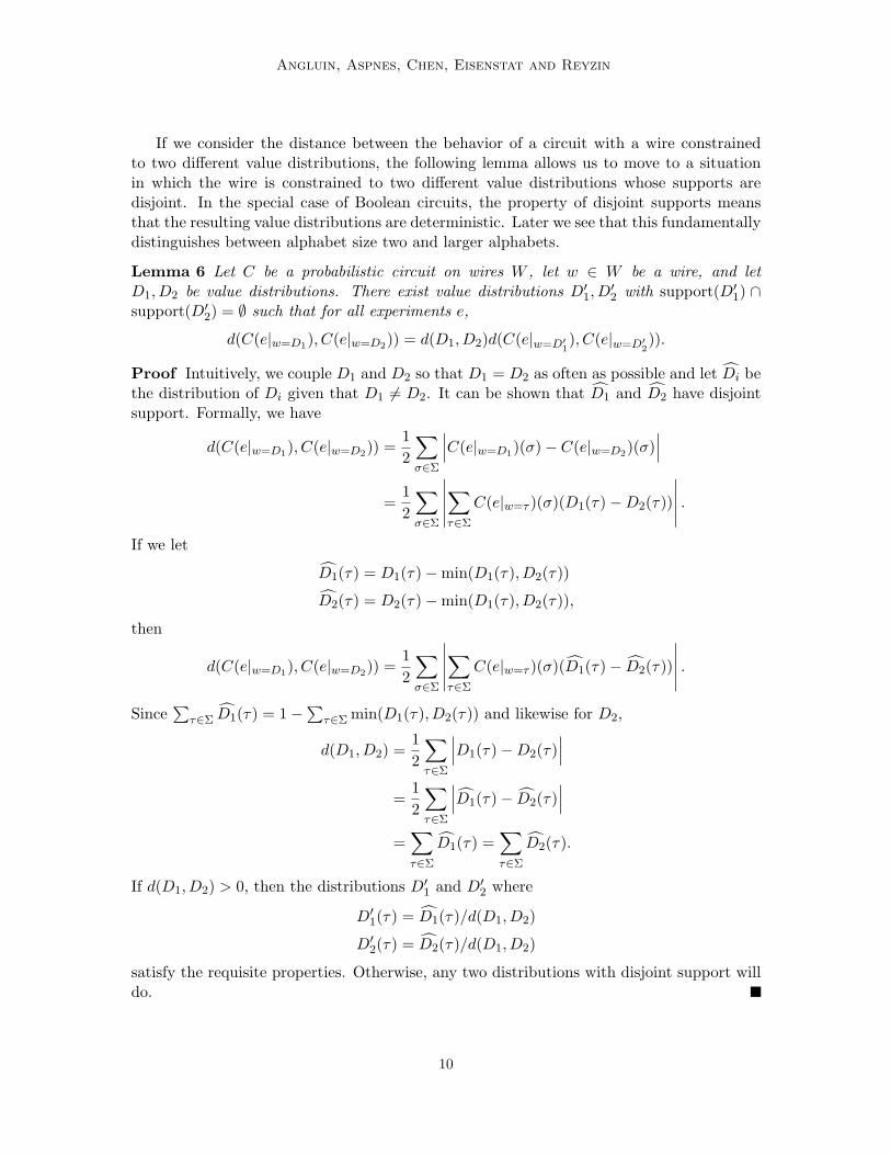
If we consider the distance between the behavior of a circuit with a wire constrainedto two different value distributions, the following lemma allows us to move to a situationin which the wire is constrained to two different value distributions whose supports aredisjoint. In the special case of Boolean circuits, the property of disjoint supports meansthat the resulting value distributions are deterministic. Later we see that this fundamentallydistinguishes between alphabet size two and larger alphabets.
Lemma 6 Let C be a probabilistic circuit on wires W , let w ∈ W be a wire, and letD1, D2 be value distributions. There exist value distributions D′1, D
′2 with support(D′1) ∩
support(D′2) = ∅ such that for all experiments e,
d(C(e|w=D1), C(e|w=D2)) = d(D1, D2)d(C(e|w=D′1), C(e|w=D′
2)).
Proof Intuitively, we couple D1 and D2 so that D1 = D2 as often as possible and let Di bethe distribution of Di given that D1 6= D2. It can be shown that D1 and D2 have disjointsupport. Formally, we have
d(C(e|w=D1), C(e|w=D2)) =12
∑σ∈Σ
∣∣∣C(e|w=D1)(σ)− C(e|w=D2)(σ)∣∣∣
=12
∑σ∈Σ
∣∣∣∣∣∑τ∈Σ
C(e|w=τ )(σ)(D1(τ)−D2(τ))
∣∣∣∣∣ .If we let
D1(τ) = D1(τ)−min(D1(τ), D2(τ))
D2(τ) = D2(τ)−min(D1(τ), D2(τ)),
then
d(C(e|w=D1), C(e|w=D2)) =12
∑σ∈Σ
∣∣∣∣∣∑τ∈Σ
C(e|w=τ )(σ)(D1(τ)− D2(τ))
∣∣∣∣∣ .Since
∑τ∈Σ D1(τ) = 1−
∑τ∈Σ min(D1(τ), D2(τ)) and likewise for D2,
d(D1, D2) =12
∑τ∈Σ
∣∣∣D1(τ)−D2(τ)∣∣∣
=12
∑τ∈Σ
∣∣∣D1(τ)− D2(τ)∣∣∣
=∑τ∈Σ
D1(τ) =∑τ∈Σ
D2(τ).
If d(D1, D2) > 0, then the distributions D′1 and D′2 where
D′1(τ) = D1(τ)/d(D1, D2)
D′2(τ) = D2(τ)/d(D1, D2)
satisfy the requisite properties. Otherwise, any two distributions with disjoint support willdo.
10

Learning Acyclic Probabilistic Circuits Using Test Paths
4. Test Paths
The concept of a test path has been central in previous work on learning deterministiccircuits by means of value injection queries (Angluin et al., 2008b, 2009). A test path fora wire w, or w-test path, is a value injection experiment in which the free gates form adirected path in the circuit graph from w to the output wire. All the other wires in thecircuit are fixed; this includes the inputs of w. A side wire with respect to a test path pis a wire fixed by p that is input to a free wire in p.
As an example, suppose that Σ = {0, 1} and the target circuit has a circuit graphas shown in Figure 2. There are four directed paths from w1 to the output wire: w1w5,w1w3w5, w1w2w4w5 and w1w3w4w5. A w1-test path is a value injection experiment thatsets the wires of one of these paths to ∗ and the other wires to 0 or 1, for example, ∗011∗ or∗∗0∗∗. For the test path ∗011∗, the side wires are w3 and w4, while for the test path ∗∗0∗∗the side wire is w3. The value injection experiments ∗∗∗∗∗ and ∗01∗∗ are not test paths.
w1
w2 w3
w5
w4
Figure 2: A circuit graph; w5 is the output wire.
A test path may help the learning algorithm determine the effects of assigning differentvalues to the wire w. The test path lemmas (Angluin et al., 2008b, 2009) may be re-statedas follows.
Lemma 7 Let C be a deterministic circuit. If for some value injection experiment e, wirew free in e and alphabet symbols σ and τ it is the case that
C(p|w=σ) = C(p|w=τ )
for every test path p ≤ e then also
C(e|w=σ) = C(e|w=τ ).
11
Angluin, Aspnes, Chen, Eisenstat and Reyzin
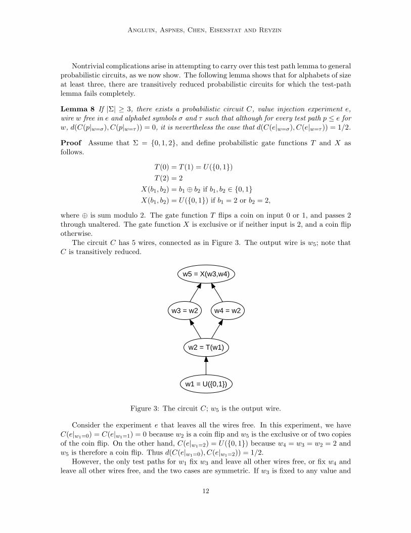
Nontrivial complications arise in attempting to carry over this test path lemma to generalprobabilistic circuits, as we now show. The following lemma shows that for alphabets of sizeat least three, there are transitively reduced probabilistic circuits for which the test-pathlemma fails completely.
Lemma 8 If |Σ| ≥ 3, there exists a probabilistic circuit C, value injection experiment e,wire w free in e and alphabet symbols σ and τ such that although for every test path p ≤ e forw, d(C(p|w=σ), C(p|w=τ )) = 0, it is nevertheless the case that d(C(e|w=σ), C(e|w=τ )) = 1/2.
Proof Assume that Σ = {0, 1, 2}, and define probabilistic gate functions T and X asfollows.
T (0) = T (1) = U({0, 1})T (2) = 2
X(b1, b2) = b1 ⊕ b2 if b1, b2 ∈ {0, 1}X(b1, b2) = U({0, 1}) if b1 = 2 or b2 = 2,
where ⊕ is sum modulo 2. The gate function T flips a coin on input 0 or 1, and passes 2through unaltered. The gate function X is exclusive or if neither input is 2, and a coin flipotherwise.
The circuit C has 5 wires, connected as in Figure 3. The output wire is w5; note thatC is transitively reduced.
w1 = U({0,1})
w2 = T(w1)
w3 = w2 w4 = w2
w5 = X(w3,w4)
Figure 3: The circuit C; w5 is the output wire.
Consider the experiment e that leaves all the wires free. In this experiment, we haveC(e|w1=0) = C(e|w1=1) = 0 because w2 is a coin flip and w5 is the exclusive or of two copiesof the coin flip. On the other hand, C(e|w1=2) = U({0, 1}) because w4 = w3 = w2 = 2 andw5 is therefore a coin flip. Thus d(C(e|w1=0), C(e|w1=2)) = 1/2.
However, the only test paths for w1 fix w3 and leave all other wires free, or fix w4 andleave all other wires free, and the two cases are symmetric. If w3 is fixed to any value and
12

Learning Acyclic Probabilistic Circuits Using Test Paths
all other wires are free, then w5 is a coin flip when w1 = 2. If w3 is fixed to 2 and allother wires are free, then w5 is also a coin flip. If w3 is fixed to b ∈ {0, 1} and all otherwires are free, then when w1 ∈ {0, 1}, w2 is a coin flip, and w5 is the exclusive or of b andthat coin flip, that is, w5 is also coin flip. Hence, for any test path p ≤ e for w1, we haveC(p|w1=0) = C(p|w1=2) = U({0, 1}) and d(C(pw1=0), C(pw1=2)) = 0.
For alphabets Σ of size larger than 3, we can treat three of the symbols as 0, 1 and 2 inthe above construction, and the other symbols as “tilt,” where each function outputs a tiltvalue if any of its inputs is a tilt value.
4.1 A Bound for Boolean Probabilistic Circuits
Surprisingly, the case of |Σ| = 2 is different; for Boolean probabilistic circuits there is auseful quantitative relationship between the difference exposed by an arbitrary experimente and the differences exposed by test paths p ≤ e. The bound we give depends on thestructure of directed paths on free wires in e.
Let e be an experiment and w a wire. Define Π(e, w) to be the set of all directed pathsfrom w to the output wire on free wires in e. Let S(e) be the set of wires that originate afree shortcut, that is, the set of free wires w such that there exists a path p ∈ Π(e, w) withtwo free wires to which w is an input. Define
κ(e, w) =∑
p∈Π(e,w)
2|p∩S(e)|.
Thus, κ(e, w) is the sum over paths in Π(e, w) of 2 raised to the number of wires on thepath that originate free shortcuts in e. If there are no wires that originate free shortcuts ine, then this is just the number of free paths in e. As an example, if the target circuit hasthe circuit graph shown in Figure 2 and the experiment e leaves all wires free then Π(e, w1)contains the four paths w1w5, w1w3w5, w1w2w4w5 and w1w3w4w5, S(e) = {w1, w3}, andκ(e, w) is 2 + 4 + 2 + 4 = 12.
The following technical lemma gives a useful recurrence for κ(e, w).
Lemma 9 Let C be a probabilistic circuit, e be a distribution injection experiment, w andu be free wires where w is an input to u, and D0 be a value distribution. Let β = 2 ifw ∈ S(e) and β = 1 otherwise. Then
κ(e, w) = κ(e|u=D0 , w) + κ(e|w=1, u) · β.
13

Angluin, Aspnes, Chen, Eisenstat and Reyzin
Proof The first term of the sum counts paths that don’t contain u, and the second countspaths that do. Let e′ = e|u=D0 and e′′ = e|w=1. We have
κ(e, w) =∑
p∈Π(e,w)
2|p∩S(e)|
=∑
p∈Π(e,w)u6∈p
2|p∩S(e)| +∑
p∈Π(e,w)u∈p
2|p∩S(e)|
=∑
p∈Π(e′,w)
2|p∩S(e′)| +∑
p∈Π(e′′,u)
2|p∩S(e′′)|β
= κ(e′, w) + κ(e′′, u) · β,
since each path p 3 u from w corresponds to the path p \ {w} from u.
Next is the key lemma relating the difference exposed by e to the differences exposed bypaths p ≤ e for Boolean probabilistic circuits.
Lemma 10 Let C be a Boolean probabilistic circuit, e be a distribution injection experi-ment, w be a wire free in e and D1, D2 be value distributions. If there exists ε ≥ 0 such thatfor all w-test paths p ≤ e,
d(C(p|w=D1), C(p|w=D2)) ≤ ε,
thend(C(e|w=D1), C(e|w=D2)) ≤ κ(e, w) · ε.
Proof By induction on φ(e), the number of free wires in e. By Lemma 6, assume thatsupport(D1) ∩ support(D2) = ∅. The critical feature of the Boolean case is that it followsthat D1 = 0 and D2 = 1 without loss of generality—it is important to the following proofthat D1 and D2 be deterministic.
If φ(e) = 1, then eitherd(C(e|w=0), C(e|w=1)) = 0,
or w is the output, e is a w-test path, and κ(e, w) = 1. Otherwise, the inductive hypothesisis that the lemma holds for all experiments e′ with φ(e′) < φ(e).
Except for w, the experiments e|w=0 and e|w=1 agree on all constrained wires, so byLemmas 4 and 5, assume without loss of generality that every wire with no free path fromw is in fact fixed. Since C is acyclic, there exists a free wire u 6= w whose only unfixedinput is w. Let g be the gate assigned by C to u and let B0 = g(e|w=0) and B1 = g(e|w=1),so that
C(e|w=0) = C(e|w=0,u=B0)C(e|w=1) = C(e|w=1,u=B1).
By the triangle inequality,
d(C(e|w=0), C(e|w=1)) ≤ d(C(e|w=0,u=B0), C(e|w=1,u=B0))+ d(C(e|w=1,u=B0), C(e|w=1,u=B1)).
14
Learning Acyclic Probabilistic Circuits Using Test Paths
Letting e′ = e|u=B0 , any test path p ≤ e′ also satisfies p ≤ e since e′ ≤ e. The experimente′ has one fewer free wire, as u is free in e, so using the inductive hypothesis, we can boundthe first term of the sum by κ(e′, w) · ε. We now derive a bound on u-test paths so that theinductive hypothesis applies to the second term as well. Let β = 2 if w ∈ S(e) and β = 1otherwise. Let e′′ = e|w=1 and suppose p ≤ e′′ is a u-test path. Then
d(C(p|u=B0), C(p|u=B1))≤ d(C(p|w=1,u=B0), C(p|w=0,u=B0)) + d(C(p|w=0,u=B0), C(p|w=1,u=B1))[by the triangle inequality]= d(C(p|w=1,u=B0), C(p|w=0,u=B0)) + d(C(p|w=0,u=∗), C(p|w=1,u=∗))
[by the definitions of B0 and B1].
Since w is an input to u, both p|w=∗,u=B0 and p|w=∗,u=∗ are w-test paths. Therefore, bothterms of the sum are bounded by ε, and the first is nonzero only if w is an input to somefree wire in p other than u. It follows that
d(C(p|u=B0), C(p|u=B1)) ≤ βε,
and thus that
d(C(e′′|u=0), C(e′′|u=1)) ≤ κ(e′′, u) · βε,
so by Lemma 9,
d(C(e|w=0), C(e|w=1)) ≤ κ(e′, w) · ε+ κ(e′′, u) · βε= κ(e, w) · ε.
In the case of transitively reduced circuits, S(e) = ∅, and κ(e, w) = π(e, w), whereπ(e, w) = |Π(e, w)|, the number of directed paths on free wires in e from w to the outputwire.
Corollary 11 Let C be a transitively reduced Boolean probabilistic circuit, e be a distribu-tion injection experiment, and w be a wire free in e. If there exists ε ≥ 0 such that for allw-test paths p ≤ e,
d(C(p|w=0), C(p|w=1)) ≤ ε,
thend(C(e|w=0), C(e|w=1)) ≤ π(e, w) · ε.
5. Learning Boolean Probabilistic Circuits
The amount of attenuation given by Lemma 10 allows us to adapt the Circuit Builderalgorithm (Angluin et al., 2009) to learn Boolean probabilistic circuits with constant fan-inand log depth in polynomial time. For this class of circuits, the attenuation factor κ(e, w)is bounded by a polynomial in n.
15

Angluin, Aspnes, Chen, Eisenstat and Reyzin
Theorem 12 Given constants c and k there is a nonadaptive learning algorithm that withprobability at least (1−δ) successfully ε-approximately learns any Boolean probabilistic circuitwith n wires, gates of fan-in at most k and depth at most c log n using value injection queriesin time bounded by a polynomial in n, 1/ε and log(1/δ).
The rest of the section is devoted to proving this theorem. Let the target circuit be Cwith Σ = {0, 1} and let positive constants δ, ε, k and c be given such that the fan-in of Cis bounded by k and the depth of C is bounded by c log n. For such a circuit, π(e, w) isbounded above by kc logn, so the quantity κ(e, w) is bounded above by
κ(n) = kc logn · 2c logn = nc(log k+1) = nO(1).
We now describe our Probabilistic Circuit Builder algorithm (PCB). PCB is nonadap-tive: first it computes a set U of value injection experiments such that every test path isequivalent to some experiment in U . It then repeats each value injection query e ∈ U enoughtimes that with probability at least (1−δ), the distribution C(e) is estimated with sufficientaccuracy for every e ∈ U . Finally, it uses these estimates to build a circuit C ′ by repeatedlyadding a sufficiently accurate gate all of whose inputs are in the partially constructed circuit.If the estimates of C(e) are all sufficiently accurate, then C ′ is ε-behaviorally equivalent toC.
5.1 Constructing U
In choosing the experiments U , the goal is that for every potential test path, U includesan equivalent experiment. The structure of the circuit, however, is not known a priori, adifficulty that we overcome by the same method as used by Angluin et al. (2009). Let U∗be a universal set of value injection experiments such that for every set of kc log n wires andevery assignment of symbols from Σ ∪ {∗} to those wires, some experiment e ∈ U∗ agreeswith the values assigned to those wires. There is a deterministic construction of such a setU∗ of size
2O(kc logn) log n = nO(kc)
in time polynomial in its size (Angluin et al., 2009). (For intuition, a set of nO(kc) indepen-dent random uniform assignments of ∗, 0 and 1 to the wires has this property with highprobability.) For every wire w and test path p for w, there is an experiment in U∗ that leavesthe path wires of p free and fixes the side wires of p to their values in p. Consequently, pand this experiment agree on the output wire. In order to have experiments in which eachfree wire is also set to 0 and 1, for b = 0, 1 let Ub contain every experiment e|w=b such thate ∈ U∗ and w is free in e. The final set of experiments is U = U∗ ∪ U0 ∪ U1.
5.2 Estimating C(e) for e ∈ U
For each e ∈ U , PCB repeatedly makes a value injection query with e to estimate the valuedistribution C(e); let C(e) denote this estimate. By Hoeffding’s bound, we have that
m = O((nκ(n)/ε)2 log(|U |/δ))
trials per experiment e suffice to guarantee that with probability at least 1−δ, for all e ∈ U ,
d(C(e), C(e)) ≤ ε/(4nκ(n)). (1)
16
Learning Acyclic Probabilistic Circuits Using Test Paths
Let e ∈ U∗ be a value injection experiment, w be a wire that e leaves free, and D be a valuedistribution. We define
C(e|w=D) =∑σ∈Σ
D(σ)C(e|w=σ).
Note that this is computed from the values of C(e|w=σ) and does not require new experi-ments.
If (1) holds for all e ∈ U , then we have
d(C(e|w=D), C(e|w=D)) ≤∑σ∈Σ
D(σ)d(C(e|w=σ), C(e|w=σ))
≤ ε/(4nκ(n)). (2)
5.3 Building the circuit C ′
PCB builds the circuit C ′ one gate at a time. Let W ′ denote the set of wires of C ′ that havealready been assigned a gate by PCB; initially W ′ is empty. While W ′ 6= W , PCB attemptsto add another gate to C ′ by searching for a wire w ∈ (W −W ′) and a probabilistic gate g′
all of whose inputs are in W ′ such that for each experiment e ∈ U∗ that leaves w free andfixes all inputs of g′,
d(C(e), C(e|w=g′(e))) ≤ 2ε/(4nκ(n)).
If no such gate can be found or W ′ = W , PCB outputs C ′ and halts. We will later showthat a gate can be found as long as W 6= W ′.
The search for g′ iterates over every wire w ∈ (W − W ′) and every choice of an r-tuple of distinct wires w1, . . . , wr from W ′ as the inputs of w, where 0 ≤ r ≤ k. For eachsuch choice, PCB attempts to define a probabilistic gate function f as follows. For each(σ1, . . . , σr) ∈ Σr, PCB seeks a number x ∈ [0, 1] such that if Dx is the distribution that is1 with probability x and 0 with probability (1− x) then
d(C(e), C(e|w=Dx)) ≤ 2ε/(4nκ(n))
for all experiments e ∈ U∗ that leave w free and fix wi to σi for i = 1, . . . , r. Since the lefthand side is a convex function of x, every such e constrains the possible values of x to aninterval, and any x in the intersection of [0, 1] and the intervals for all such e suffices. If theintersection is empty, then the attempt to define f fails; otherwise, f(σ1, . . . , σr) is definedto be Dx. If PCB succeeds in defining f for all possible r-tuples (σ1, . . . , σr), then the gateg′ with inputs w1, . . . , wr and probabilistic gate function f is assigned to w.
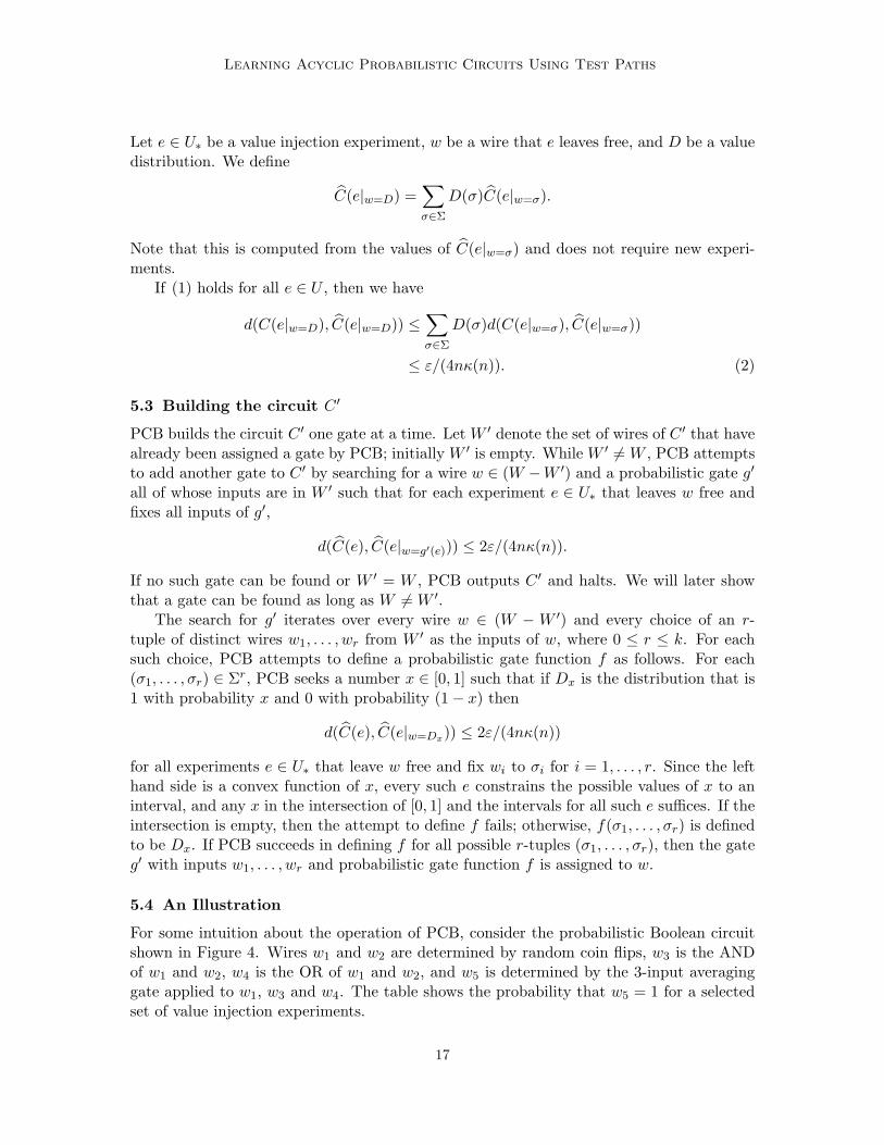
5.4 An Illustration
For some intuition about the operation of PCB, consider the probabilistic Boolean circuitshown in Figure 4. Wires w1 and w2 are determined by random coin flips, w3 is the ANDof w1 and w2, w4 is the OR of w1 and w2, and w5 is determined by the 3-input averaginggate applied to w1, w3 and w4. The table shows the probability that w5 = 1 for a selectedset of value injection experiments.
17
Angluin, Aspnes, Chen, Eisenstat and Reyzin
w1 = U({0,1}) w2 = U({0,1})
w3 = w1 /\ w2 w4 = w1 \/ w2
w5 = A(w1,w3,w4)# Experiment Pr[w5 = 1]1. * * * * * 1/22. 0 * * * * 1/63. 1 * * * * 5/64. * * 0 * * 5/125. * * 1 * * 3/46. * 1 * 0 * 1/37. 0 1 * 0 * 08. 1 1 * 0 * 2/39. * 1 0 0 * 1/6
10. * 1 1 0 * 1/2
Figure 4: A Boolean circuit with output wire w5, and some of its behavior.
Suppose that these experiments are contained in U when PCB attempts to add the firstgate to C ′. Of course, PCB will only have repeated sampling estimates of these probabilities,but suppose for a moment that the exact values were available. Because W ′ is empty, thefirst gate added must have no inputs and must be determined by a coin flip that is 1 withsome probability x. In this group of experiments, there are two constraints for wire w1 for thepossible values of x. Experiments 1, 2 and 3 give the constraint (1/6)(1−x)+(5/6)x = 1/2,which implies x = 1/2, and experiments 6, 7 and 8 give the constraint 0(1−x)+(2/3)x = 1/3,which also implies x = 1/2, consistent with the gate computing w1 in the target circuit.There are also two constraints on the possible values of x for the wire w3. Experiments1, 4 and 5 give the constraint (5/12)(1 − x) + (3/4)x = 1/2, which implies x = 1/4, andexperiments 6, 9 and 10 give the constraint (1/6)(1 − x) + (1/2)x = 1/3, which impliesx = 1/2. Thus there is no consistent value of x that would allow the first gate to bechosen for wire w3. Rather than exact values, PCB considers intervals determined by errortolerances, but when these are small enough, the constraint intervals for w3 will not overlap,and PCB will not choose the first gate for wire w3.
5.5 Correctness
With probability at least (1 − δ), the estimates C(e) satisfy (1) for all e ∈ U . We nowassume that the estimates satisfy these bounds and show that PCB successfully builds acircuit C ′ that is ε-behaviorally equivalent to C.
We first establish two lemmas connecting gates, paths and experiments. Given a Booleanprobabilistic circuit C and a probabilistic gate g, g is η-correct for wire w with respectto C if for every value injection experiment e that fixes the input wires for g we haved(C(e), C(e|w=g(e))) ≤ η, where g(e) denotes the value distribution determined by g whenits inputs are fixed as in e. Recall that φ(e) denotes the number of free wires in experimente, and therefore φ(e) ≤ n for all e.
Lemma 13 Let C and C ′ be probabilistic circuits on wires W , and let e be a distributioninjection experiment. If for every wire w, the gate for w in C ′ is η-correct for w with respect
18

Learning Acyclic Probabilistic Circuits Using Test Paths
to C, then
d(C(e), C ′(e)) ≤ φ(e) · η.
Proof By induction on φ(e), the number of free wires in e. If φ(e) = 0, then e constrainsthe output wire, and trivially, d(C(e), C ′(e)) = 0. Otherwise, the inductive hypothesis isthat
d(C(e′), C ′(e′)) ≤ φ(e′) · η
for all experiments e′ with fewer than φ(e) free gates.By Lemma 2, assume that e is in fact a value injection experiment. Since C ′ is acyclic,
there exists a free wire w in e such that the inputs to w in C ′ are fixed in e to some k-tuple(σ1, . . . , σk) ∈ Σk. Let f denote the probabilistic gate function for w in C ′, and let D denotethe value distribution f(σ1, . . . , σk). Then we have C ′(e) = C ′(e|w=D), and
d(C(e), C ′(e)) ≤ d(C(e), C(e|w=D)) + d(C(e|w=D), C ′(e|w=D))≤ η + (φ(e)− 1) · η= φ(e) · η
by the inductive hypothesis and the fact that f is η-correct for w.
Corollary 14 Let C and C ′ be probabilistic circuits on wires W where |W | = n. If forevery wire w, the gate g for w in C ′ is η-correct for w with respect to C, then
d(C(e), C ′(e)) ≤ n · η.
Proof By the definition of approximate behavioral equivalence and the bound φ(e) ≤ n.
Next we show that test paths are sufficient to determine whether a gate is η-correct fora wire in C.
Lemma 15 Let C be a Boolean probabilistic circuit, w a wire and g′ a probabilistic gate.If for every test path p for w that fixes all the inputs of g′, d(C(p), C(p|w=g′(p))) ≤ η/Kw,where Kw is the maximum value of κ(e, w) for C over all experiments e, then g′ is η-correctfor w with respect to C.
Proof Let g be the actual gate that C assigns to w. Let e be a value injection experimentthat fixes every input of g′. Then e may not fix all of g’s inputs, but because C is acyclic,g’s inputs are not reachable from w. By Lemmas 4 and 5, there exists an experiment e′ ≤ ethat fixes g’s inputs, with
d(C(e′), C(e′|w=g′(e′))) ≥ d(C(e), C(e|w=g′(e))).
19

Angluin, Aspnes, Chen, Eisenstat and Reyzin
Since e′ fixes all of g’s inputs, C(e′) = C(e′|w=g(e′)). It is given that for all test paths p thatfix all inputs of g′ that
d(C(p|w=g(p)), C(p|w=g′(p))) ≤ η/Kw,
so it follows by Lemma 10 that
d(C(e′|w=g(e′)), C(e′|w=g′(e′))) ≤ κ(e′, w) · η/Kw ≤ η,
and g′ is η-correct for w.
To prove that PCB constructs a circuit C ′ that is ε-behaviorally equivalent to the targetcircuit C, we show that for each wire w ∈W , PCB assigns a gate that is ε/n-correct for win C.
Assume that W ′ 6= W , that is, that not all wires have been assigned gates, and considerPCB as it attempts to add another gate to C ′. PCB looks for a wire w ∈ (W −W ′) andprobabilistic gate g′ ∈ G with all of its inputs in W ′ such that for each experiment e ∈ U∗that leaves w free and fixes all inputs of g′,
d(C(e), C(e|w=g′(e))) ≤ 2ε/(4nκ(n)).
If this search succeeds, then by (1),
d(C(e), C(e)) ≤ ε/(4nκ(n))d(C(e|w=g′(e)), C(e|w=g′(e))) ≤ ε/(4nκ(n)),
and thus by the triangle inequality we have
d(C(e|w=g′(e)), C(e)) ≤ ε/(nκ(n)),
It follows by Lemma 15 and the choice of κ(n) that g′ is ε/n-correct for w in C.To see that the search for a gate will succeed as long as W ′ 6= W , we note that because
C is acyclic, there is some wire w ∈ (W −W ′) such that all of w’s inputs in C are in W ′.Let g denote the gate assigned by C to w, with inputs w1, . . . , wr and probabilistic gatefunction f . By the existence of g, there is at least one feasible gate-wire assignment forPCB to make, ensuring the continued progress of PCB. Consider any experiment e ∈ U∗that leaves w free and fixes the inputs of g to (σ1, . . . , σr). Let D be the value distributionf(σ1, . . . , σr). Then C(e) = C(e|w=D) and by (1) and (2) we have
d(C(e), C(e)) ≤ ε/(4nκ(n))
d(C(e|w=D), C(e|w=D)) ≤ ε/(4nκ(n)),
so by the triangle inequality,
d(C(e), C(e|w=D)) ≤ 2ε/(4nκ(n)).
Therefore, PCB will continue to make progress until it has assigned a gate to every wire inW , and every such gate will be ε/n-correct for its wire in C, which means that C ′ will beε-behaviorally equivalent to C.
20

Learning Acyclic Probabilistic Circuits Using Test Paths
5.6 Running time
To bound the running time of PCB we argue as follows. The set U of experiments is ofcardinality nO(kc) and can be constructed in time polynomial in its size. To estimate C(e),each experiment in U is repeated
O((nκ(n)/ε)2 log(|U |/δ))
times; recall that κ(n) = O(nc(log k+1)). PCB then chooses a gate for a wire n times. Foreach choice, it must at worst iterate over O(n) wires in (W −W ′), over all O(nk) choices ofk or fewer input wires from W ′, over all |Σ|k assignments of values to the input wires, andall experiments in U . Thus the running time of PCB is polynomial in n, 1/ε and 1/δ.
6. Lower Bounds on Path Attenuation
The path attenuation bound κ(n) is a significant factor in the running time of the PCBalgorithm. In this section we consider lower bounds on path attenuation for Boolean prob-abilistic circuits. The following theorem shows that the bound of π(e, w) for transitivelyreduced Boolean probabilistic circuits in Corollary 11 is tight infinitely often.
Theorem 16 There is an infinite set of transitively reduced probabilistic Boolean circuitssuch that for each circuit C in the family, there exists a value injection experiment e and awire w free in e such that
d(C(e|w=0), C(ew=1)) = 1
and for every test path p for w we have
d(C(p|w=0), C(p|w=1)) = 1/π(e, w).
Proof For each positive integer `, define the circuit C` to be a chain of ` copies of thecircuit C1 in Figure 1 with wire w4 of one copy identified with wire w1 of the next copy.More formally, the 3` + 1 wires are w0,4 and wi,j for i = 1, . . . , ` and j = 2, 3, 4. Theoutput wire is w`,4. The wire w0,4 has no inputs and is determined by an unbiased coinflip, that is, U({0, 1}). The wires wi,2 and wi,3 are the outputs of deterministic identitygates with input wi−1,4. The wire wi,4 = A(wi,2, wi,3) is the result of applying the two-inputaveraging probabilistic gate function A to the wires wi,2 and wi,3. The circuit C3 is depictedin Figure 5.
To understand the operation of this circuit in response to a value injection experimente, we may view each averaging gate as choosing one of its inputs to copy to its output.Starting at the output wire, this determines a path back to the first wire whose value hasbeen fixed, or to the wire w0,4 (which has no inputs) and the output of the circuit is thevalue of the wire so reached.
Define experiment e to leave all of the wires free. Let w denote the wire w0,4. Clearlythere are 2` paths on free gates in e from w to the output gate, that is, π(w, e) = 2`. For ex-periment e every possible path starts at wire w and we have C(e|w=0) = 0 and C(e|w=1) = 1,so d(C(e|w=0), C(e|w=1)) = 1. However, any test path p for w must fix one of the wires wi,2or wi,3 for each i = 1, . . . , `. Thus, there is exactly one path that leads back to wire w, andthis path is the one chosen by the averaging gates with probability 1/2`. Thus the result
21

Angluin, Aspnes, Chen, Eisenstat and Reyzin
w04 = U({0,1})
w12 = w04 w13 = w04
w14 = A(w12,w13)
w22 = w14 w23 = w14
w24 = A(w22,w23)
w32 = w24 w33 = w24
w34 = A(w32,w33)
Figure 5: The circuit C3; w3,4 is the output wire.
22

Learning Acyclic Probabilistic Circuits Using Test Paths
for any test path p for w is d(C(p|w=0), C(p|w=1)) = 1/2` = 1/π(e, w).
This lower bound also holds for general transitively reduced circuit topologies, as follows.(Note that this result was incorrectly stated in the preliminary version of this paper (Angluinet al., 2008a).)
Theorem 17 Let G be a transitively reduced acyclic directed graph with a designated outputnode z that is reachable from every node. For each node w there exists a Boolean probabilisticcircuit C whose circuit graph is G with output wire z such that for every value injectionexperiment e that leaves w free and for every test path p ≤ e for wire w we have
d(C(e|w=1), C(e|w=0)) ≥ π(e, w) · d(C(p|w=1), C(p|w=0)).
Proof Let w be given. To construct C, each node v of G is assigned a probabilistic gatewhose inputs are the in-neighbors of v in G, as follows. For each node v, let P (v) denotethe number of distinct directed paths from w to z that include node v, and for each edge(u, v), let P (u, v) denote the number of distinct directed paths from w to z that includeedge (u, v). If there are no paths from w to z through v (that is, P (v) = 0) then we let theprobabilistic gate function for v be the constant function 0. The probabilistic gate functionfor w is a coin flip, U({0, 1}).
Otherwise, if node v has inputs u1, . . . , ur then it is assigned the probabilistic gatefunction specified by
Av(b1, . . . , br) =r∑i=1
bi · P (ui, v)/P (v)
This generalizes the two-input averaging gate A, weighting input ui by the fraction of pathsfrom w to z passing through v that also pass through ui. We may view Av as performinga random weighted selection of one of its inputs to copy to its output. The weights havebeen chosen so that each directed path from w to z is selected with probability 1/P (w).
Let e be any value injection experiment that leaves w free. If there is no path on freewires in e from w to the output, then π(e, w) = 0, and the bound in the conclusion of thelemma holds trivially. Otherwise, the output of the circuit in response to e is determinedby tracing from the output wire, following the choices of the averaging gates, until eitherthe first wire fixed by e, or w, is reached. Thus
d(C(e|w=1), C(e|w=0)) = π(e, w)/P (w),
because there are π(e, w) paths from w to the output wire in e. Let p ≤ e be any test pathfor w; now there is just one choice of path that leads back to w, so
d(C(p|w=1), C(p|w=0)) = 1/P (w),
establishing the conclusion of the lemma.
Can the general bound in Lemma 10 be improved to the bound for transitively reducedcircuits in Corollary 11? The following example shows that the better bound is in general
23
Angluin, Aspnes, Chen, Eisenstat and Reyzin
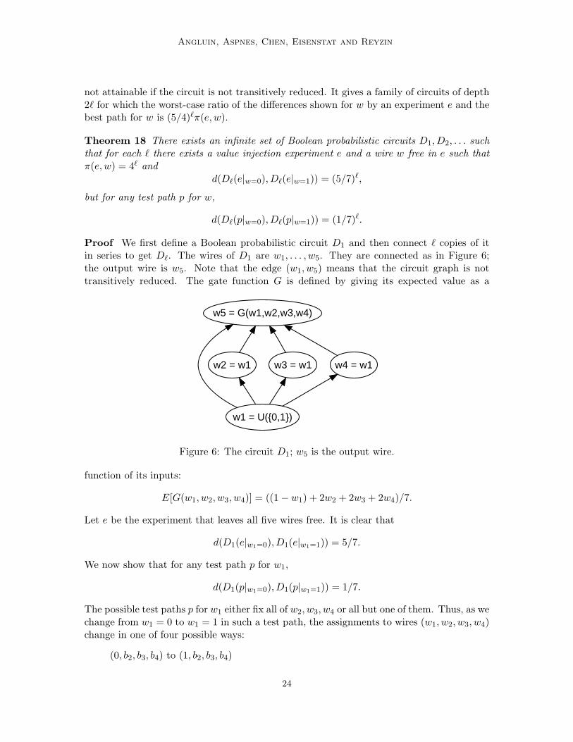
not attainable if the circuit is not transitively reduced. It gives a family of circuits of depth2` for which the worst-case ratio of the differences shown for w by an experiment e and thebest path for w is (5/4)`π(e, w).
Theorem 18 There exists an infinite set of Boolean probabilistic circuits D1, D2, . . . suchthat for each ` there exists a value injection experiment e and a wire w free in e such thatπ(e, w) = 4` and
d(D`(e|w=0), D`(e|w=1)) = (5/7)`,
but for any test path p for w,
d(D`(p|w=0), D`(p|w=1)) = (1/7)`.
Proof We first define a Boolean probabilistic circuit D1 and then connect ` copies of itin series to get D`. The wires of D1 are w1, . . . , w5. They are connected as in Figure 6;the output wire is w5. Note that the edge (w1, w5) means that the circuit graph is nottransitively reduced. The gate function G is defined by giving its expected value as a
w1 = U({0,1})
w2 = w1 w3 = w1 w4 = w1
w5 = G(w1,w2,w3,w4)
Figure 6: The circuit D1; w5 is the output wire.
function of its inputs:
E[G(w1, w2, w3, w4)] = ((1− w1) + 2w2 + 2w3 + 2w4)/7.
Let e be the experiment that leaves all five wires free. It is clear that
d(D1(e|w1=0), D1(e|w1=1)) = 5/7.
We now show that for any test path p for w1,
d(D1(p|w1=0), D1(p|w1=1)) = 1/7.
The possible test paths p for w1 either fix all of w2, w3, w4 or all but one of them. Thus, as wechange from w1 = 0 to w1 = 1 in such a test path, the assignments to wires (w1, w2, w3, w4)change in one of four possible ways:
(0, b2, b3, b4) to (1, b2, b3, b4)
24

Learning Acyclic Probabilistic Circuits Using Test Paths
(0, 0, b3, b4) to (1, 1, b3, b4)
(0, b2, 0, b4) to (1, b2, 1, b4)
(0, b2, b3, 0) to (1, b2, b3, 1)
Checking each of these possible changes against the definition of G, we see that each changeproduces a difference of 1/7, as claimed. (This example can be modified to give a differenceof 1 versus 1/5.) Thus, setting w = w1, the circuit D1 gives the base case of the claim inthe lemma.
To construct D`, we take ` copies of D1 and identify wire w5 in one copy with wire w1
in the next copy, making the wire w5 of the final copy the output wire of the whole circuit.Let w denote the wire w1 in the first such copy. Then π(e, w) = 4` and
d(D`(e|w=0), D`(ew=1)) = (5/7)`.
For any test path p, the signal is attenuated by a factor of 1/7 for each level, and we have
d(D`(p|w=0), D`(p|w=1)) = 1/7`.
This construction can be generalized to k+1 wires for any odd k+1, which increases theattenuation. In the base circuit there are k paths and an attenuation factor of 1/(2k − 3),and the worst-case ratio of differences for an experiment and its test paths in D` approaches2`π(e, w) as k goes to infinity.
7. Exponential Dependence on Depth
The bounds on path attenuation show that test paths may be much less informative thangeneral value injection experiments, resulting in the exponential dependence of the numberof experiments and the running time of PCB on the depth of the target circuit. It is naturalto ask whether we might do better by using selected general experiments. In this section, wegive computational evidence to the contrary. The following result contrasts with the case ofdeterministic circuits, where the Distinguishing Paths algorithm uses value injection queriesto learn arbitrary transitively reduced acyclic deterministic circuits of constant fan-in overpolynomial size alphabets in polynomial time (Angluin et al., 2008b).
Theorem 19 If BPP 6= NP and k ≥ 4 then there is no polynomial time algorithm usingvalue injection queries that approximately learns all acyclic transitively reduced Booleanprobabilistic circuits with fan-in bounded by k.
Proof Suppose L is a polynomial time algorithm that approximately learns the behavior ofevery transitively reduced acyclic Boolean probabilistic circuit of fan-in bounded by 4 usingvalue injection queries. The hard computational problem we consider is the following: givena satisfiable 3-CNF formula φ over the variables x1, . . . , xn with clauses c1, . . . , cm, find anassignment to the variables that satisfies significantly more than seven-eights of the clauses
25
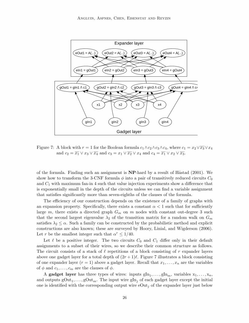
Angluin, Aspnes, Chen, Eisenstat and Reyzin
Gadget layer
Expander layer
gIn1 gIn2
x1
gOut1 = gIn1 /\ c1
gIn3
x2
gOut2 = gIn2 /\ c2
gIn4
x3
gOut3 = gIn3 /\ c3
x4
gOut4 = gIn4 /\ c4
eIn1 = gOut1 eIn2 = gOut2 eIn3 = gOut3 eIn4 = gOut4
eOut1 = A(...) eOut2 = A(...) eOut3 = A(...) eOut4 = A(...)
Figure 7: A block with r = 1 for the Boolean formula c1∧c2∧c3∧c4, where c1 = x2∨x3∨x4
and c2 = x1 ∨ x3 ∨ x4 and c3 = x1 ∨ x2 ∨ x4 and c4 = x1 ∨ x2 ∨ x3.
of the formula. Finding such an assignment is NP-hard by a result of Hastad (2001). Weshow how to transform the 3-CNF formula φ into a pair of transitively reduced circuits C0
and C1 with maximum fan-in 4 such that value injection experiments show a difference thatis exponentially small in the depth of the circuits unless we can find a variable assignmentthat satisfies significantly more than seven-eighths of the clauses of the formula.
The efficiency of our construction depends on the existence of a family of graphs withan expansion property. Specifically, there exists a constant α < 1 such that for sufficientlylarge m, there exists a directed graph Gm on m nodes with constant out-degree 3 suchthat the second largest eigenvalue λ2 of the transition matrix for a random walk on Gmsatisfies λ2 ≤ α. Such a family can be constructed by the probabilistic method and explicitconstructions are also known; these are surveyed by Hoory, Linial, and Wigderson (2006).Let r be the smallest integer such that αr ≤ 1/40.
Let ` be a positive integer. The two circuits C0 and C1 differ only in their defaultassignments to a subset of their wires, so we describe their common structure as follows.The circuit consists of a stack of ` repetitions of a block consisting of r expander layersabove one gadget layer for a total depth of (2r+ 1)`. Figure 7 illustrates a block consistingof one expander layer (r = 1) above a gadget layer. Recall that x1, . . . , xn are the variablesof φ and c1, . . . , cm are the clauses of φ.
A gadget layer has three types of wires: inputs gIn1, . . . , gInm, variables x1, . . . , xn,and outputs gOut1, . . . , gOutm. The input wire gInj of each gadget layer except the initialone is identified with the corresponding output wire eOutj of the expander layer just below
26

Learning Acyclic Probabilistic Circuits Using Test Paths
it. The variable wires xi of each gadget layer have no inputs and default to the constant 0.Each output wire gOutj has four inputs: the corresponding gadget input wire gInj and thethree variable wires for the variables of the clause cj of φ. Its gate function computes theconjunction of gInj and the value of the clause cj given its three variable values.
Thus, if the learner sets the variable wires xi in a gadget layer according to a satisfyingassignment of φ, the signals propagate from the gadget inputs gInj to their correspondingoutputs gOutj with perfect fidelity. Otherwise, any unsatisfied clause blocks the signal forthe corresponding output.
An expander layer averages the outputs of the layer below to be the inputs for thelayer above, according to the expander graph Gm. Each input eInj of an expander layer isset equal to the corresponding output of the gadget or expander layer immediately belowit. The three inputs to eOutj are eInk for the three out-neighbors k of j in the expandergraph Gm. The gate function for each eOutj is the three-input averaging gate A(x, y, z),which is 1 with probability (x+y+ z)/3. The output of the whole circuit is the first outputwire of the final (topmost) expander layer.
The initial inputs are the input wires gInj of the initial gadget layer. They have noinputs; for the circuit C0 they are all assigned the default value 0, and for the circuit C1
they are all assigned the default value 1. Note that C0 and C1 are transitively reduced andhave a maximum fan-in of 4.
The challenge for the learner is to determine which of C0 and C1 is the target circuit. Ifa value injection experiment succeeds in setting the variable wires in every gadget layer to(possibly different) satisfying assignments for the formula φ and leaves all other wires free,then the output of C0 is 0 and the output of C1 is 1. If not all the clauses of φ are satisfied,then this distance is reduced.
Intuitively, the learner’s strategy must be to fix the variable wires in each gadget layerto prevent the signal from the initial inputs from getting blocked; fixing the input or outputwires of gadget or expander layers would not help, because they would then have the samevalue regardless of their inputs. Without a good variable assignment, however, the signalstrength drops by a constant factor for each layer, as we now show.
Let e be a value injection experiment. The experiment e induces an assignment to thevariables of φ for each gadget layer, either by fixing the value of each variable wire or lettingit default to 0. The effect of an averaging gate is to select one of its inputs at random andcopy the value of that input to the output. Thus, the output of the circuit for experimente is in effect determined by a random walk backward from the output wire until the walkreaches a wire whose value is fixed by e (and the output is the fixed value), or a gadgetlayer output wire corresponding to an unsatisfied clause (and the output is 0), or an initialinput wire (and the output is the value of that wire.) Suppose that for each gadget layer eencodes a variable assignment that satisfies at most (9/10)m of the clauses of φ. We showthat the probability that the random walk hits an initial input wire is bounded above by(39/40)`
√m.
Without loss of generality we may assume that e fixes no wires other than variable wiresand initial input wires, because any other fixed wires reduce the probability of reaching aninitial input. For i = 1, . . . , `, let Wi be the m×m diagonal matrix with 1s for each satisfiedclause in the ith gadget layer and 0s for each unsatisfied clause. Let B be the transitionmatrix for an r-step random walk on Gm and let e1 = (1, 0, . . . , 0). The probabilities of the
27
Angluin, Aspnes, Chen, Eisenstat and Reyzin
random walk hitting the initial inputs are given by the vector e1BW`BW`−1 · BW2BW1.By the following argument, for all i and vectors v, we have ‖vBWi‖ ≤ (39/40)‖v‖.
Write v = cu + w, where c is a scalar and u = (1, . . . , 1) and w is a vector suchthat u ⊥ w. Then u is an eigenvector of B with eigenvalue 1 and multiplying w by Bshrinks its length to at most the second eigenvalue of B times its original length. ByPythagoras, ‖cu‖ ≤ ‖v‖ and ‖w‖ ≤ ‖v‖. We have vBWi = (cu + w)BWi. On one hand,‖cuBWi‖ = ‖cuWi‖ ≤
√9/10‖cu‖ ≤ (19/20)‖v‖. On the other hand, ‖wB‖ ≤ (1/40)‖v‖,
because the second eigenvalue of B is no larger than 1/40, and ‖wBWi‖ ≤ (1/40)‖v‖,because Wi does not increase the L2 norm. The resulting (39/40)` bound on the L2 normof the probability vector gives a bound of (39/40)`
√m on the L1 norm, which is an upper
bound on the probability that any initial input is reached.Suppose the learning algorithm L runs in time f(N, 1/ε, 1/δ), for some nondecreasing
polynomial f , where N is the number of wires in the target circuit. Let N(`) denote thenumber of wires in C0 (or C1) as a function of the number ` of blocks in the stack. ThenN(`) = O(`(n+ rm)). We choose ` sufficiently large that
((39/40)`√m)f(N(`), 4, 4) < 1/4,
clearly N(`) is bounded by a polynomial in m and n.We randomly and equiprobably choose the target circuit C to be C0 or C1 and simulate
L with target circuit C and ε = δ = 1/4. When L makes a value injection experiment e,we check whether any of the induced variable assignments of e satisfies more than (9/10)mclauses of φ. If so, we output the assignment and halt. Otherwise, we use a random walkfrom the output wire in the circuit C to give an output for e. If no experiment e satisfiesmore than (9/10)m of the clauses of φ, then the probability that any of them reaches aninitial input in C is less than 1/4. If none of them reaches an initial input, then L cannotdistinguish between C0 and C1, and must output a circuit that is not 1/4-approximatelybehaviorally equivalent to C with probability at least 3/8 > 1/4, violating the requirementsof approximate learning.
We conclude that if BPP 6= NP, any polynomial time learning algorithm requires inexpectation exponentially many queries in ` to learn the default settings of the initial inputsand therefore, PCB is within a polynomial of optimal.
8. Non-Boolean Circuits Revisited
The sharp contrast in results for transitively reduced circuits with alphabet size at leastthree, for which test paths may show no difference (Lemma 8) and those with alphabetsize two, for which test paths must show a significant difference (Lemma 10) motivate usto consider a generalization of the kinds of experiments we consider, to function injectionexperiments. This generalization allows us to extend the results of Lemma 10 to non-Boolean alphabets.
In a value injection experiment, each wire is either fixed to a constant value or leftfree. In a function injection experiment for a wire w, these possibilities are expanded topermit a transformation of the value that the wire w would take if it were left free. As
28

Learning Acyclic Probabilistic Circuits Using Test Paths
an example, consider a transformation in which the values that w could attain are linearlyordered and all values below a certain threshold are mapped to the minimum value andall other values are mapped to the maximum value. It is conceivable that this kind oftransformation could be feasible in some domains; in any case, the theoretical consequencesare quite interesting. We first give a general definition of function injection, but in theresults below we are primarily concerned with 2-partitions, that is, transformations thatare like the above example in that they partition the values into at most two blocks andmap each block to a fixed element of the block.
An alphabet transformation is a function f that maps symbols to distributionsover symbols. An alphabet transformation is deterministic if it assigns only deterministicdistributions, in which case we think of it as a map from symbols to symbols. A deterministicalphabet transformation f is a k-partition if there exists a partition of Σ into at most kdisjoint nonempty sets Σi such that for each i there exists σi ∈ Σi such that f(Σi) = {σi}.Note that if k1 ≤ k2, every k1-partition is also a k2-partition.
A 1-partition is a constant function, achieving the same result as fixing the wire toa value in a value injection experiment. We use 2-partitions to reduce the case of largeralphabets to the binary case. Note that the 2-partitions of a binary alphabet include theidentity and the two constant functions, but not the negation function.
If D is a value distribution and f is an alphabet transformation, then f(D) is the valuedistribution in which
(f(D))(σ) =∑τ∈Σ
D(τ)(f(τ))(σ).
A function injection experiment is a mapping e with domain W that assigns to eachwire the symbol ∗ or a symbol from Σ or an alphabet transformation f . Then e leaves w freeif e(w) = ∗, fixes w if e(w) ∈ Σ, and transforms w if e(w) is an alphabet transformation f .We extend the ordering ≤ on experiments by stipulating that each alphabet transformationf ≤ ∗. A 2-partition experiment is a function injection experiment in which everyalphabet transformation is a 2-partition.
We now define the joint probability distribution on assignments of symbols from Σ towires determined by a function injection experiment e. If e fixes w, then w is just assignede(w). Otherwise, if the inputs of w have been assigned the values σ1, . . . , σk and f is thegate function for w, we randomly and independently choose a symbol σ according to thevalue distribution f(σ1, . . . , σk). If w is free in e, then σ is the symbol assigned to w;however, if e(w) is an alphabet transformation, then a symbol τ is chosen randomly andindependently according to the value distribution e(σ) and assigned to w. That is, whene(w) is an alphabet transformation, we generate the symbol for w as though it were free,and then use the distribution e(w) to transform that symbol. Because C is acyclic, thisprocess assigns a symbol to every wire of C.
In a function injection query (FIQ), the learning algorithm gives a function injectionexperiment e and receives a symbol σ assigned to the output wire of C by the probabilitydistribution defined above. A functional test path for a wire w is a function injectionexperiment in which the free and transformed wires are a directed path in the circuit graphfrom w to the output wire, and all other wires are fixed.
29

Angluin, Aspnes, Chen, Eisenstat and Reyzin
As an example of how functional test paths help in learning non-Boolean probabilisticcircuits, consider again the circuit in the proof of Lemma 8, depicted in Figure 3. Wespecify a functional test path p by p(w1) = p(w4) = p(w5) = ∗, p(w3) = 0 and p(w2) is thealphabet transformation 0→ 0, 1→ 0, and 2→ 2. Note that the alphabet transformationis a 2-partition. Then C(p|w1=0) = 0 but C(p|w1=2) = U({0, 1}), so this functional testpath witnesses a difference of 1/2, as large as the experiment that leaves all the wires free.Test paths with functions allow us to carry over the results of Lemma 10 to non-Booleanalphabets.
Lemma 20 Let C be a probabilistic circuit, e be a function injection experiment, w be awire free in e and D1, D2 be value distributions. If there exists ε ≥ 0 such that for allfunctional w-test paths p ≤ e that are 2-partitions,
d(C(p|w=D1), C(p|w=D2)) ≤ ε,
thend(C(e|w=D1), C(e|w=D2)) ≤ κ(e, w) · ε.
Proof The obstacle in Lemma 10 is that when the alphabet is non-Boolean, we mayassume only that D1 and D2 have disjoint support, not that they are deterministic. Thisobstacle can be overcome by injecting a 2-partition at w. Let Σ1 = support(D1) andΣ2 = support(D2) and assume Σ1 ∩ Σ2 = ∅. Then
d(C(e|w=D1), C(e|w=D2)) ≤∑ρ1∈Σ1ρ2∈Σ2
D1(ρ1)D2(ρ2)d(C(e|w=ρ1), C(e|w=ρ2))
by the triangle inequality. Let
(σ, τ) = arg maxρ1∈Σ1ρ2∈Σ2
d(C(e|w=ρ1), C(e|w=ρ2))
so that
d(C(e|w=D1), C(e|w=D2)) ≤ d(D1, D2)d(C(e|w=σ), C(e|w=τ )).
Let f be an alphabet transformation that maps Σ1 to σ and Σ2 to τ and all other symbolsto either σ or τ . Then f is a 2-partition, and
d(C(e|w=D1), C(e|w=D2)) ≤ d(C(e|w=f(D1)), C(e|w=f(D2))).
Since f(D1) = σ and f(D2) = τ , the rest of the proof goes through.
Corollary 21 Let C be a transitively reduced probabilistic circuit, e be a function injectionexperiment, w be a wire, and D1, D2 be value distributions. If there exists ε ≥ 0 such thatfor all functional w-test paths p ≤ e,
d(C(p|w=D1), C(p|w=D2)) ≤ ε,
thend(C(e|w=D1), C(e|w=D2)) ≤ π(e, w) · ε.
30
Learning Acyclic Probabilistic Circuits Using Test Paths
We expect that a further generalization of the Probabilistic Circuit Builder algorithmto use function injection experiments can learn non-Boolean circuits of logarithmic depthand constant fan in in polynomial time. The universal set would map wires to the setcontaining all alphabet symbols from Σ and all 2-partitions of Σ, of which there are fewerthan |Σ|22|Σ|. Thus, the universal set will still be of size nO(1), suggesting that a polynomialtime algorithm may be attainable in this case.
Certain other natural questions arise in response to the idea of function injection ex-periments. We can define circuits C and C ′ to be strongly behaviorally equivalent ifC(e) = C ′(e) for every function injection query e. Does behavioral equivalence imply strongbehavioral equivalence? Once again, alphabet size determines the answer: no for alphabetsize greater than two, yes for alphabet size two.
Lemma 22 For Σ = {0, 1, 2}, there exist deterministic circuits C1 and C2 that are behav-iorally equivalent but not strongly behaviorally equivalent.
Proof In both C1 and C2 there are two wires w1 and w2, where w2 is the output wire. Inboth circuits the gate for w2 has input w1 and deterministically maps 0 to 0 and maps 1and 2 to 1. In C1, w1 is the constant 1 and C2 it is the constant 2.
Then if e is the value injection experiment that leaves both wires free, C1(e) = 1 = C2(e).If e fixes either w1 or w2, then also C1(e) = C2(e). Thus C1 is behaviorally equivalent toC2.
However, the 2-partition function injection experiment e that leaves w2 free and mapsthe output of w1 according to the transformation 0→ 0, 1→ 0, 2→ 2 yields C1(e) = 0 andC2(e) = 1. Thus C1 is not strongly behaviorally equivalent to C2.
However, 2-partition function experiments suffice to establish strong behavioral equiva-lence.
Lemma 23 Let C and C ′ be probabilistic circuits with the same alphabet Σ, the same set ofwires and the same output wire. If C(e) = C ′(e) for every 2-partition function experimente then C and C ′ are strongly behaviorally equivalent.
Proof By a generalization of the Probabilistic Circuit Builder algorithm to functional testpaths.
Because in the Boolean case every 2-partition function injection query is a value injectionquery, we then have the following.
Corollary 24 For Boolean probabilistic circuits C and C ′, if C is behaviorally equivalentto C ′ then C is strongly behaviorally equivalent to C ′.
9. Discussion and Open Problems
These results concern general probabilistic acyclic gates, with no restriction other than fan-in on the kinds of probabilistic gate functions considered. Particular domains may warrantspecific assumptions about the gate functions, which may make the learning problems more
31
Angluin, Aspnes, Chen, Eisenstat and Reyzin
tractable. For example, for the problem of learning the structure of an independent cascadesocial network using exact value injection queries, a query-optimal algorithm is presentedby Angluin et al. (2008c). Note that social networks may in general contain cycles, whichcomplicates their analysis.
The Distinguishing Paths algorithm (Angluin et al., 2008b) learns transitively reducedacyclic deterministic circuits over polynomial size alphabets with constant fan-in and nodepth bound using value injection queries in polynomial time, and relies on a version ofthe test path lemma. Theorem 19 shows that if BPP 6= NP then this algorithm doesnot generalize to arbitrary transitively reduced Boolean probabilistic circuits, but there isa possibility that it might generalize to transitively reduced Boolean probabilistic circuitswith a polynomial bound on the total number of directed paths in the circuit graph. Asomewhat technical open question is whether in the case of general Boolean probabilisticcircuits, the ability to inject the NOT function might reduce the maximum path attenuationto just the number of paths, as it does in the case of the circuit in Figure 6.
Acknowledgments
James Aspnes acknowledges the support of NSF grant CNS-0435201. This work wasdone while Jiang Chen was a member of the Center for Computational Learning Systems,Columbia University; he acknowledges the support of a research contract from ConsolidatedEdison. Lev Reyzin acknowledges that this material is based upon work supported undera National Science Foundation Graduate Research Fellowship. A preliminary version ofthis paper was presented at COLT 2008 (Angluin et al., 2008a). The authors thank thereviewers of the COLT 2008 version of the paper and the referees of the present paper fortheir thoughtful comments.
References
Tatsuya Akutsu, Satoru Kuhara, Osamu Maruyama, and Satoru Miyano. Identification ofgenetic networks by strategic gene disruptions and gene overexpressions under a booleanmodel. Theor. Comput. Sci., 298(1):235–251, 2003.
Dana Angluin and Michael Kharitonov. When won’t membership queries help? J. Comput.Syst. Sci., 50(2):336–355, 1995.
Dana Angluin, James Aspnes, Jiang Chen, David Eisenstat, and Lev Reyzin. Learningacyclic probabilistic circuits using test paths. In Twenty-First Annual Conference onLearning Theory, pages 169–179. Omicron, July 2008a.
Dana Angluin, James Aspnes, Jiang Chen, and Lev Reyzin. Learning large-alphabet andanalog circuits with value injection queries. Machine Learning, 72(1-2):113–138, 2008b.
Dana Angluin, James Aspnes, and Lev Reyzin. Optimally learning social networks withactivations and suppressions. In Nineteenth International Conference on AlgorithmicLearning Theory, volume 5254 of Lecture Notes in Computer Science, pages 272–286,October 2008c.
32
Learning Acyclic Probabilistic Circuits Using Test Paths
Dana Angluin, James Aspnes, Jiang Chen, and Yinghua Wu. Learning a circuit by injectingvalues. J. Comput. Syst. Sci., 75(1):60–77, 2009.
N. Friedman, M. Linial, I. Nachman, and D. Pe´er. Using Bayesian networks to analyzeexpression data. J. Comput. Biol., 7(3–4):601–620, 2000.
Johan Hastad. Some optimal inapproximability results. J. ACM, 48(4):798–859, 2001.
Shlomo Hoory, Nathan Linial, and Avi Wigderson. Expander graphs and their applications.Bull. Amer. Math. Soc. (N.S.), 43(4):439–561 (electronic), 2006.
T. Ideker, V. Thorsson, and R Karp. Discovery of regulatory interactions through pertur-bation: Inference and experimental design. In Pacific Symposium on Biocomputing 5,pages 302–313, 2000.
David Kempe, Jon M. Kleinberg, and Eva Tardos. Maximizing the spread of influencethrough a social network. In KDD ’03: Proceedings of the Ninth ACM SIGKDD Interna-tional Conference on Knowledge Discovery and Data Mining, pages 137–146, New York,NY, USA, 2003. ACM.
David Kempe, Jon M. Kleinberg, and Eva Tardos. Influential nodes in a diffusion modelfor social networks. In ICALP, pages 1127–1138, 2005.
Judea Pearl. Causality: Models, Reasoning, and Inference. Cambridge University Press,2000.
33