SETTING BOUNDARIES: MONITORING THE EFFECTS OF CLOSER-TO-HOME

SCHOOL REZONING ON STUDENT PARTICIPATION

& ENGAGEMENT IN SCHOOL

By

Kristie J. Rowley

Dissertation

Submitted to the Faculty of the

Graduate School of Vanderbilt University

In partial fulfillment of the requirements

For the degree of

DOCTOR OF PHILOSOPHY

in

Leadership and Policy Studies

December, 2005

Greensville, Tennessee

Approved:

Professor Ellen B. Goldring

Professor Thomas M. Smith

Professor Mark Berends

Professor Claire Smrekar

Professor Adam Gamoran

TABLE OF CONTENTS

Page LIST OF TABLES...............................................................................................................v LIST OF FIGURES ........................................................................................................... vi Chapter I. INTRODUCTION...................................................................................................1 II. SENSE OF PLACE & SOCIAL DISORGANIZATION: A CONCEPTUAL FRAMEWORK 10 The sociology of community and sense of place ............................................12 Community and sense of place defined ..............................................16 Social disorganization theory..........................................................................22 Social disorganization and research on neighborhood effects............28 Criticisms of social disorganization theory ........................................29 Schools as mediators...........................................................................30 Conceptual model............................................................................................33 III. THE RETURN TO NEIGHBORHOOD SCHOOL & THE CASE OF METRO GREENSVILLE .....................................................................................39 Brown and the legal history of race in education............................................39 Responses to court-ended segregation ............................................................42 The case of Greensville: The road to unitary status ........................................47 Unitary status ......................................................................................49 IV. DATA & METHODS............................................................................................52 Data .................................................................................................................53 District data.........................................................................................53 Census data .........................................................................................58 Teacher survey data ............................................................................59 Measures .........................................................................................................61 Outcome variables ..............................................................................62 Background variables .........................................................................67 Neighborhood/school zone context variables .....................................69 Mediating variable ..............................................................................72 School characteristics constructs from the Greensville Teacher Survey .................................................................................................74

ii

Analyses ..........................................................................................................83 Cross-classified growth models ..........................................................84 Methodological considerations...........................................................86 V. CHANGES IN SCHOOLS & ZONES OVER TIME............................................94 Changes in school characteristics over time ...................................................95 Zoned school trends............................................................................95 Enhanced option school trends ...........................................................97 Change in school neighborhoods and school zones over time........................99 Residential stability ............................................................................99 Ethnic diversity.................................................................................103 Family disruption..............................................................................105 Social advantage ...............................................................................107 Economic deprivation.......................................................................109 School zone distance.........................................................................110 Differences between enhanced options and zoned schools...........................117 Enhanced options vs. all other zoned schools ..................................117 Enhanced options vs. similar zoned schools.....................................119 VI. RESULTS............................................................................................................123 Results from cross-classified growth models................................................123 Number of student absences .............................................................126 Number of disciplinary events..........................................................136 Climate of enhanced option schools .............................................................146 Climate of enhanced options vs. zoned schools ...............................147 Stability of enhanced option school climate .....................................150 VII. CONCLUSIONS.................................................................................................156 Main findings ................................................................................................156 When schools are closer to home .....................................................157 Neighborhoods matter ......................................................................157 The role of enhanced option schools ................................................159 Implications for education policy..................................................................160 Implications for social science research........................................................163 Appendix A. SAMPLE OF STUDNETS BY YEAR, GRADE, AND SCHOOL TYPE .........167 B. TEACHER SURVEY ..........................................................................................171 C. HLM & HCM MODEL NOTATION & EQUATIONS......................................190

iii

D1. DESCRIPTION OF SCHOOL ZONE CONTEXTS OVER TIME ....................191 D2. DESCRIPTION OF SCHOOL ZONE CONTEXTS OVER TIME ....................209 REFERENCES ................................................................................................................227

iv

LIST OF TABLES Table Page 1. Sample of Students & Schools Compared to District Totals for All Years ..........57 2. Description of Variables........................................................................................64 3. Description of Teacher Survey Variables..............................................................75 4. Distribution of Dependent Variables.....................................................................87 5. Bivariate Correlations of School-Level Variables ................................................92 6. Description of School-Level Changes Over Time ................................................96 7. Description of Change in the Contexts of School Zones over Time...................101 8. Description of Change in the Number of Block Groups Associated with a School Zone over Time ....................................................................................113 9. Description of Change in the Distance Between Home & School over Time.............................................................................................................115 10. Hierarchical Linear Growth Model Predicting Change in Size of School Attendance Zones over Time...............................................................................116 11. Independent Sample T-Tests Describing Mean Differences Between Enhanced Option Schools and Zoned Schools ....................................................118 12. Independent Sample T-Tests Describing Mean Differences Between Enhanced Option Schools and Demographically Similar Zoned Schools...........121 13. Cross-Classified Models Predicting Student Absenteeism..................................127 14. Cross-Classified Models Predicting Student Discipline ......................................137 15. Comparison of Enhanced Option Schools to a Sample of Zoned Schools in 2004 .................................................................................................................148 16. Longitudinal Comparison of Enhanced Option Schools from 2002 to 2004 .................................................................................................................151 17. Longitudinal Comparison of Zoned Schools from 2002 to 2004 ........................154

v

LIST OF FIGURES Figure Page 1. Conceptual Model for the Mediation of Neighborhood Effects............................36 2. Trends in the Residential Stability of School Zones Experiencing the Largest Changes from 1999 to 2004 ..............................................................102 3. Trends in the Ethnic Diversity of School Zones with the Largest Changes from 1999 to 2004.................................................................................104 4. Trends in the Family Disruption of School Zones with the Largest Changes from 1999 to 2004.................................................................................106 5. Trends in the Social Advantage of School Zones with the Largest Changes form 1999 to 2004.................................................................................108 6. Trends in the Economic Deprivation of School Zones with the Largest Changes from 1999 to 2004.................................................................................111 7. Direct Effects of School Zone Distance & Enhanced Option Schools on Student Attendance .........................................................................................130 8. School Zone Contexts & Student Attendance .....................................................132 9. Direct Effects of School Zone Distance & Enhanced Option Schools on Student Discipline...........................................................................................142 10. School Zone Contexts & Student Discipline .......................................................143 11. Comparison of Trends in Enhanced Option Schools & Zoned Schools over Time .............................................................................................................152

vi

CHAPTER I

INTRODUCTION

This dissertation addresses the role of community resources in the recent trend

toward the establishment of neighborhood schools. Community resources tend to be

geographically distributed; therefore, resources such as social, human, and economic

capital are not equally present in all neighborhoods and subsequently, they are not

equally present in all school attendance zones. A trend toward neighborhood schools

could mark a perpetuation of inadequate and inequitable educational opportunities for

students living in disadvantaged neighborhoods. This relationship between neighborhood

resources and their effects on student outcomes is addressed within the context of the

Greensville Metropolitan Public Schools (GMPS, or Metro), an urban, Southeastern

school district recently declared unitary after decades of court-ordered desegregation.

A grant of “unitary status” is the legal term, and actually, a legal status of a school

district that has, according to a federal court, achieved to the extent practicable the court’s

requirements for desegregation. A unitary school system is one in which the segregative

practices of the former dual system are no longer evident and no longer affect current

operations. When a district is declared unitary, racial balancing and the associated cross-

town busing practices are generally replaced with elaborate student re-assignment plans

involving a return to neighborhood schools, or schools that are closer to students’ homes.

This reorganization of urban schooling represents a significant shift in priorities—it

introduces an era where past priorities of racial balancing are superceded by a renewed

1

emphasis on sending children to schools that are closer to their homes. This shift is

prevalent across most urban school districts that have been declared unitary (Orfield,

2001).

Because most diverse, urban school districts are residentially segregated, a return

to neighborhood schools often marks a return to segregated schools—schools segregated

by both race and socioeconomic status (Frankenber, Lee, & Orfield, 2003; Frankenberg

& Lee, 2002; Orfield & Eaton, 1996). As school districts move from court-ordered to

court-ended desegregation, monitoring the tensions between the sense of place that

neighborhood schools are intended to foster and the potential effects of the

geographically-based distribution community resources, or lack thereof, becomes

paramount.

In theory, a return to neighborhood schools offers the possibility for increased

participation in schools for both parents and students, increased community attachment,

and more time and opportunities for extra-curricular activities. When students and

parents live close to their schools, participation may be less time consuming and may be

less of a burden on families. Therefore, schools may be better able to act as centers for

community life and address needs specific to the geographic area they serve. Some also

argue that neighborhood schools offer possibilities for increased social capital, as schools

can become a center for community life and interaction (Goldring & Crowson, 2002;

Driscoll, 2001). In the case of high-poverty, re-segregated schools, this increase in social

capital could most likely come from targeted social services, community outreach

programs, additional school resources, and other compensatory education strategies

designed to meet the needs of students living in particular neighborhoods. The

2

underlying assumption is that residents living in certain neighborhoods have specific

needs in terms of education and schooling, and those needs can best be met within the

context of a specific community. The work of James Comer (1980) provides support for

this model of community-based educational interventions. His intervention program was

implemented in two schools in New Haven, Connecticut and both schools demonstrate

the power of community-based schools in providing the necessary resources for

communities to invest in schools and in education, thereby enhancing the social capital of

students, parents, and communities (Comer, 1980).

As early as 1966, Coleman’s and his colleagues’ research on educational

resources and student achievement demonstrated no relationship between most school-

level resources and student achievement on standardized tests. The variable that did have

the greatest, positive relationship with student achievement was the composition of the

school’s student population. Students from low-income populations reached significantly

higher achievement levels when they attended schools where a majority of students came

from middle- or upper-income populations. When school composition was mostly low

income, students did not perform as well. Recent work has confirmed Coleman’s

findings (see Sampson & Raudenbush, 1999; Furstenberg, Cook, Eccles, Elder, &

Sameroff, 1999).

More recently, Catsambis and Beveridge (2001) found that characteristics of

disadvantaged neighborhoods and schools impact student achievement both directly and

indirectly. Specifically, neighborhoods characterized by concentrated disadvantage and

schools characterized by student poverty and absenteeism tended to depress students’

achievement in mathematics. There was also an indirect relationship between

3

neighborhood and school disadvantage and student achievement: disadvantaged

neighborhoods were found to be related to the absence of parental practices (i.e., parents’

ability to help with homework and other forms of parental involvement) that are

associated with high mathematics achievement. “Place of residence,” according to

Catsambis and Beveridge (2001) “may have important consequences for the academic

success and the resulting life chances of adolescents. Place of residence may affect

minority students the most, because they are concentrated in inner-city, disadvantaged

neighborhoods” (p. 24; also see Massey & Denton, 1993). Such studies provide evidence

that disadvantaged neighborhoods lack resources that are important for determining the

educational success of children, and as such, students attending neighborhood schools in

disadvantaged neighborhoods do not perform as well as students who live in more

advantaged neighborhoods.

In reaction to these findings and in an attempt to provide more equitable

education in terms of peer effects, several school districts across the country have

adopted intricate student assignment plans that consider a student’s socioeconomic status

as either a mechanism for drawing school zones (for example, Wake County North

Carolina) or a tool for controlling school choice (such as, Charleston South Carolina and

Boston Massachusetts). While well intended, these plans discount the possibility that

neighborhood schools may offer students and parents—especially students and parents

from low-income areas with limited access to transportation—greater opportunities for

involvement and participation, thereby creating a more consistent and stable environment

that may be important for students. Nevertheless, evaluations of these student assignment

plans suggest that they result in higher student achievement (measured by performance

4

on standardized tests), particularly for students from lower socioeconomic backgrounds

(Willie, 1990; Willie, Alves, & Hagerty, 1996; Willie, Alves, & Mitchell, 1998).

It is important to note, however, that most of the research documenting the

negative effects of disadvantaged communities on student outcomes considers academic

achievement as the only outcome of interest. Regardless, it is possible for neighborhood

schools to act as a positive force in the lives of residents in disadvantaged neighborhoods

in other ways. When using more community-based outcomes to evaluate school

effectiveness—outcomes such as students’ social engagement and participation in

schools—some suggest that neighborhood schools can contribute to an enhanced sense of

community and sense of place for children. Driscoll (2001) writes that the rediscovered

neighborhood school has a unique opportunity to help individuals reclaim a valuable

sense of place in their lives—connecting home, neighborhood, school, and community

institutions in an interactive web of sustained associations, common dreams,

expectations, and shared human and social capital.

In response to the fact that a return to neighborhood schools often results in a

return to racially segregated schools, Morris (2001) writes,

African American schools once served as the centers of close-knit communities, and in many instances, desegregation policies adversely affected African American students’ and families’ connections with their formerly all black schools. . . . Low-income, predominately black communities especially need stable institutions and for many urban communities, schools can serve this function. (p. 595; also see Kersten, 1999)

Such research supports the notion that neighborhood schools—regardless of the social,

human, and economic capital of their surrounding geographic locations—foster a greater

sense of community and improved avenues for social engagement and participation in

schools.

5

But what if the organization of some neighborhoods is not conducive to

participation and engagement in schools or in the larger community? What if “sense of

place” is never actualized in certain types of communities? What if a return to

neighborhood schools perpetuates the problems existent in disadvantaged

neighborhoods? Social disorganization theory suggests that characteristics such as

residential instability, ethnic diversity, family disruption, and poor socioeconomic

conditions impede the development of sense of place in geographic areas where such

conditions are systemic. As such, social disorganization theory questions the viability of

“community” in certain types of neighborhoods—typically, inner-city, poverty stricken

neighborhood. With neighborhood schooling, schools of concentrated poverty are

usually inevitable, and so may be the adverse effects of growing up in a disadvantaged

neighborhood. Regardless, parents and policy makers alike find value in schooling that is

closer to home. Districts are currently seeking ways to use this kind of educational

organization as a viable and favorable option for all children.

One method of facilitating the efficacy of neighborhood schools for all children is

to equip schools located in disadvantaged neighborhoods with additional resources and

support services. Full service schools, for example, have been designed with the hopes

that better schools with better resources can mediate at least some of the negative effects

of disadvantaged neighborhoods on student outcomes However, the ability of these

schools to mediate the negative effects of neighborhoods characterized by concentrated

poverty is not well understood from an empirical standpoint. Such relationships between

schools and neighborhoods have been understudied, though recent trends in closer-to-

home schooling is on the upswing despite the risk of creating racially isolated schools

6

characterized by concentrated poverty. These trends suggest that such relationships

between schools, school boundaries, and student outcomes should be explored more

rigorously.

This paper analyzes neighborhood schools, the impacts of neighborhoods on

school-related outcomes, and schools’ ability to mediate these impacts. As such, the

following three research questions are examined:

Do student participation and student engagement in school improve as

students are zoned to schools that are closer to home?

How are the neighborhood characteristics of school attendance zones

associated with student participation and engagement in school?

Are neighborhood characteristics of school attendance zones mediated when

students attend enhanced option schools (i.e., schools that provide additional

social and academic programs and resources designed to supplement the

social, human, and economic capital that is not provided in students’

neighborhoods)?

This research contributes to the investigation of educational outcomes within the

context of ever-changing social structures and their influences on communities, schools,

and individuals. Research suggests that the environment in which children grow up

affects their physical, psychological, intellectual, and social development, as well as their

opportunities for successes in life. Most educational research, however, has focused

narrowly on the effects of family and home environments on children's development and

school performance. Neighborhoods are another important part of a child's environment,

but have received comparatively less attention. Because this paper identifies school

7

attendance zones as neighborhoods, “neighborhood effects” on educational outcomes

become a mechanism that can be influenced and improved by adopting informed public

and education policies. In an era when “neighborhoods” and children’s patterns of

interactions can be politically defined by school districts as they set social priorities

through zoning patterns, an understanding of how these social boundaries affect students’

participation and engagement in school is imperative. This paper aims to inform such

policies by monitoring the influences of closer-to-home schooling in one urban school

district as their social priorities shift away from racial integration.

To study the effects of the social composition of school attendance zones on

education outcomes for student, I first outline the literature on sense of place as well as

social disorganization theory as they relate to public education and a return to

neighborhood schools. Thereafter, a brief history of the return to neighborhood schools

as it is related to the desegregation movement in the US is outlined. This history is then

extended to include Metro Greensville’s progression toward unitary status. Key to this

discussion is the context in which a return to neighborhood schools and enhanced option

schools were included as a part of Greensville’s unitary status plan. A conceptual

framework is then created from the historical context of neighborhood schools as well as

the sense of place and social disorganization literature. Measures are derived from the

literature that can be used in an analysis of neighborhood effects (and possible mediating

effects) on school outcomes. Statistical analyses are also discussed as ways to

empirically test the theories discussed in the review of literature and the relationships that

are explicated in the conceptual model. Results are then discussed and conclusions are

8

drawn as the results are linked to the sense of place and social disorganization theory

literatures as well as the policy dimensions that inform the goals of this research.

9

CHAPTER II

SENSE OF PLACE & SOCIAL DISORGANIZATION:

A CONCEPTUAL FRAMEWORK

The structure of communities and neighborhoods and their influences on the

outcomes for individuals address issues at the heart of sociology. Historically, few

concepts in sociology have played a larger or more defining role in the birth and

formation of the discipline than community. Works such as Durkheim’s (1893) The

Division of Labor in Society, Simmel’s (1983) The Metropolis and Mental Life, and

Toennies’ (1983) Gemeinschaft und Gesellschaft represent a sample of timeless works of

early sociologists who carved out the discipline with their concern about the

consequences of the changing landscape of neighborhoods and communities and its

effects on the lives of people that live within them. Nevertheless, more than a century

later, we are left with many more questions and even fewer answers about how

neighborhood and community conditions shape and influence individuals, their thoughts,

their behaviors, and their patterns of interactions. More specific to the context of this

study, several researchers have also attempted to outline the role of schools in

communities. It is theorized that neighborhoods affect local schools and that local

schools also help shape neighborhoods. These ideas have been theoretically and

empirically developed, mostly through the avenues of social research.

From these sociological traditions, two competing theories emerge as useful

lenses from which we can study the return to neighborhood schools. Research rooted in

10

community sociology identifies “sense of community,” or “sense of place,” as an

essential outcome associated with viable communities and neighborhoods (Bell &

Newby, 1972). As such, sense of place is strongly associated with social engagement and

participation. Within the context of education, it is argued that sense of place is best

obtained when schools are designed to serve the unique needs of the neighborhoods in

which they are located—whichever kinds of neighborhoods they might be (rich, poor,

White, African American, etc.) (see Driscoll, 2001; Morris, 2001).

However, social disorganization theory, a branch of the ecological model

attributed to the Chicago School, accounts for the possibility that not all neighborhoods

are created with the necessary capital (social, human, and economic) to sustain any kind

of meaningful sense of place. Research has historically found that such neighborhoods

are often located in low-income inner-cities (see Park & Burgess, 1925; Shaw & McKay,

1942; 1969). Such research suggests that neighborhood schools would be burdened by

the same organizational challenges inherent in its surrounding community—challenges

manifest mainly in the relative lack of stability and social control. However, few studies

have addressed the issue of whether or not school characteristics (such as increased,

targeted resources in high-poverty, neighborhood schools) can mediate the potentially

devastating effects of socially disorganized neighborhoods on student outcomes.1 This

study attempts to address this issue.

1 For a notable example, see Ainsworth, 2002, though this study is mainly interested in individual student motivation (and not school characteristics) as mediators of community environments.

11

The Sociology of Community & Sense of Place

Every place—regardless of its resources—embodies a unique configuration of

shared feelings, interpretations, and meanings, all of which affect one’s sense of place

(also referred to as sense of community) and one’s sense of belonging to that place. “All

places, no matter what else they have, have a sense of shared experience. And, very often,

that experience is NOT shared by other folk who do not inhabit that particular place”

(Lewis, 1979, p. 41, emphasis in original). Regardless of the levels of social, human, and

economic capital present in any given community, the experience—the sense of place—is

meaningful to those who inhabit it. Place is “a piece of the whole environment which has

been claimed by feelings” (Gussow, 1971, p.27). “Place is where, for me, community

happens” (Hummon, 1990, p. 15). When schools are tied to neighborhoods by occupying

a shared place, they are intrinsically bound to peoples’ perceptions of their community.

Therefore, neighborhood schools carry the capacity to build community by providing

avenues for social interaction and participation, social engagement, and socialization—

through the mere sharing of a common space.

Some would argue that sense of place and its ties to education have been

displaced by larger social agendas—court-ordered desegregation, for example. While

racial balance has been a noble goal, some researchers argue that the process was very

disruptive to parents’ and students’ way of life. Concerning this displacement of

community, Morris (1999) states,

In many instances today, unfortunately, a fragile connection exists between schools and African American families and communities; this was not always the case. Historically, many segregated all-Black schools were embedded in the Black community. This embeddedness—exemplified by the ways in which these schools were closely connected and interdependent with the Black community—

12

is a major reason why many African Americans viewed their schools as “good.” (p. 585; also see Irvine & Irvine, 1984; Jones, 1981; Siddle-Walker, 1993; 1996)

Additionally, researchers have demonstrated that many segregated, all-Black schools—in

spite of their typically high rates of poverty—took on unique characteristics during the

segregation era. These characteristics were reflective of the community and people they

served. They solidified the community by assisting them in the transference of similar

values and “by serving as the core focus for individual and collective aspirations” (Irvine

& Irvine, 1984, p. 416). Morris (1999) further argues that in today’s post-Brown era of

education, African American families need stability. He suggests that schools—

neighborhood schools, more specifically—can help build and sustain these same kinds of

“strong communal bonds with African American families and [become] a stabilizing

force for the community” (p. 586).

Leach (1999) agrees with the ideas addressed by Morris. He states:

A strong sense of place, along with the boundaries that shape it and give it meaning, not only fosters creativity but also helps to provide people—especially children—with an assurance that they will be protected and not abandoned . . . It is indisputable that children need a sense of place (along with an acceptance of boundaries that define and establish the safeness of place) in order to become self-reliant. (p. 179) He continues by asserting that a boundaried sense of place is the basis for

common bonding and character building. Driscoll (2001) furthers this view by

addressing the physicality, or geography, of place. She suggests that reconnecting with a

sense of place may offer insights in any movement intended to revitalize schools—

particularly schools located in high poverty, deteriorating communities. Places have

patterns—patterns of behavior, patterns of resources, patterns of ways of life. Attached

to these patterns are values. When we are able to decipher these values that we express

13

openly in our public spaces (through the patterns of our behavior), we are awakened to

the kind of respect these spaces convey for all who live and work in them. “Similarly, a

careful study of the places we educate children should tell us if the messages we convey

through them are consistent with the educational values we preach” (Driscoll, 2001, p.

25). Thus, revitalizing schooling by returning to neighborhood schools could be

beneficial, even for the poorest of communities. However, as outlined by the research on

sense of place, a mere neighborhood school will only be successful if it is coupled with a

strong commitment to aligning educational values with the patterns of life existent within

that community. That is, neighborhood schools must demonstrate a commitment and an

understanding of the needs of the community and those who inhabit it. Schools must be

established in these disadvantaged areas “as if a sense of place mattered” (Driscoll &

Kerchner, 1999; also see Gruenewald, 2003).

Although there is relatively little research dealing specifically with the effects of

neighborhoods on school-related outcomes, research using neighborhood composition to

predict other social outcomes is more plentiful. In support of the sense of place literature,

Berry, Portney, and Thomson (1991) find that poor, black residents living in

neighborhoods of concentrated poverty differ little in their political involvement from

poor, black residents living in middle-class communities. In fact, they find that “poor

people from poor neighborhoods are actually more politically active that poor people

living elsewhere” (p. 370). They found little support for the argument that

concentrations of poor blacks lead to distinctive patterns of political disengagement

(Wilson, 1987).2 Although poor blacks living in disadvantaged neighborhoods tended to

2 Berry, Portney, and Thomson’s (1991) research was based on four US cities: Birmingham, Dayton, Protland, and St. Paul. As they state in their research, the concentration of poor blacks are not as great in

14

be more cynical about their chances of influencing government than those in the

appropriate comparison groups, these attitudes seemed to be of little importance when

predicting political involvement. Berry, Portney, and Thompson (1991) attribute their

findings to the strong sense of community existent in these poor, black communities.

“Clearly, . . . neighborhoods with high concentrations of poor blacks are politically viable

communities. Poor blacks have a strong sense of community, and this characteristic

seems to help propel them into the political area” (p. 371). Thus, despite the racial and

socioeconomic makeup of “community,” shared experiences and shared conditions are

important in establishing a sense of place which is necessary for the formation of viable

neighborhoods.

American communities differ considerably in the racial, social, and economic

make-up of families living within them (Massey & Denton, 1993). It is often assumed

that poor, inner-city families that are confined to problem-ridden neighborhoods are

somehow culturally deficient. However, Furstenberg, Cook, Eccles, Elder, & Sameroff

(1999) find that these poor neighborhoods—at least in the Philadelphia area—are

occupied by families and parents whose “parenting skills, especially when measured by

the standard scales that assess warmth, commitment, discipline, and control, varied in

only trivial ways in relation to the quality of the neighborhood as measured by its

resources and social climate. Inadequate parenting . . . was far more often the exception

than the rule” (p. 217). The social and economic composition of neighborhoods made

little difference in the adequacy of parenting practices. Even the poorest of

these four cities as in some of the nation’s largest urban areas. They state, “It may be that at some greater level of concentration of poverty in black neighborhoods, political attitudes and behavior do become distinct from what would be found for other poor people and other blacks. Consequently, our data cannot categorically refute Wilson’s thesis.”

15

neighborhoods are inhabited by parents who are competent caregivers—they are neither

insensitive to their children’s need nor unskilled in meeting them. Thus, it cannot be

assumed that poor parenting is more common in poor neighborhoods, nor can it be

assumed that “community” and “sense of place” cannot be achieved in disadvantaged

neighborhoods.

Furstenberg et al. (1991) did, however, find that neighborhoods affected parents’

management strategies. Parents with greater access to material and social resources

within their communities were able to make use of collective and institutional ways of

protecting their children from negative influences and promoting their achievement.

Families living in impoverished areas, by contrast, were compelled to rely upon

individual and in-home techniques of management unless they took special steps to find

institutional resources outside their communities. Parents’ access to resources greatly

affected the range of options available to them and their children. Such resources affect

residents’ experience of community and how they interact with their environment.

Community & sense of place defined

But what is community? And where is it? The literature typically refers to sense

of place as the quintessence of “community;” thus the terms are often used

interchangeably.3 Indeed sense of place, also discussed as sense of belonging to a

particular place, seems to be dependent upon place—however subjective ones idea of

“place” or “community” may be. In spite of its historical roots in the social sciences,

“community” remains one of the most elusive concepts in sociology, and sociologists

3 As is consistent with much of the literature on “community” and “sense of place,” I also use these two terms interchangeably.

16

continue to fall short of achieving a universally accepted definition of it. It has been

defined in objective terms, as a place which occupies both time and space (Rutman &

Rutman, 1984). It has also been defined in subjective terms, as a feeling or attitude, a

state of social being, an individually unique social experience, or the network of

relationships with others regardless of place (Fischer, 1982). Some even describe

community as possessing the ability to occupy “virtual” space, such as communities

established on the internet (Rheingold, 1993; Harvard Business School, 2002). Whether

community is a physical or a virtual place, a mental construct or an objectifyable reality,

an individual experience or a collective experience, it appears that many aspects of the

experience of community—many aspects of a sense of place—seem to be unique to the

time and space in which they occupy.

In accordance with the view that any community and any experience of sense of

place is very unique to time, to place, and even to individuals, Brown, Xu, Toth, &

Nylander (1998) state that “community is a variable of personal experience in the lives of

individuals which occurs in the context of both time and space. For this reason,

community as a uniquely human condition, has been, and will continue to be difficult to

objectify” (p. 187). In part due to these inherent subjective qualities, sociologists often

seek opportunities to study communities and their influences under unique circumstances.

Generally these studies take the form of “boomtown research”—such as studies of the

changes in residents’ physical communities as well as changes in their sense of place as

they relate to the building of large scale economic developments and the occurrences of

natural disasters (see Erickson, 1976). In these conditions, the aspects of community that

17

may be taken-for-granted on a daily basis become manifest when people feel they are

threatened.

As is evident by the lack of clear, universally accepted definitions for

“community” and “sense of place,” any singular definition will fall short of describing

reality. As Pelly-Effrat (1974) describes, “Trying to study community is like trying to

scoop Jell-o up with your fingers. You can get hold of some, but there’s always more

slipping away from you” (p. 1). But this has not stopped sociologists from attempting to

define and measure community and sense of place. In one study comparing the vast array

of definitions of “community,” three aspects were held in common across 94 definitions:

geographic area, participation, and social engagement (Bell & Newby, 1972). Since there

is no widely accepted definition of community (Etzioni, 2000), I use the three

characteristics held in common across many definitions of community—geographic area,

participation, and social engagement—as necessary attributes that must be present for

“sense of place” to take hold in a community. The abstract nature of each of these

concepts which are used throughout the remainder of this work requires further

discussion.

Geographic area. Geographic area refers to boundaried space. While much of

the community literature focuses on the social benefits of the close-knit social

relationships characterized by strong communities, it does not ignore the fact that

communities are exclusive. The very nature of “sense of place” requires a firm grasp of

where the place begins and ends, who belongs and who does not. Communities, by

nature, draw lines separating member from outsiders. Cohen (1985) argues that

community boundaries are marked by two distinctive characteristics: first, members of a

18

group must have something in common with each other, and second, the thing held in

common distinguishes them in a significant way from the members of other groups.

Community, thus, implies both similarity and difference. Cohen (1985) further argues

that boundaries may be marked on a map (as administrative areas), or in law, or by

physical features (such as a river or a road). Some may be religious or linguistic.

However, not all boundaries are so obvious: “They may be though or, rather, as existing

in the minds of the beholders” (p. 12). Suttles (1972) argues that local community is best

thought of not as a single entity, but rather as a hierarchy of progressively more inclusive

residential groupings. In this sense, neighborhoods can be though of as ecological units

nested within successively larger communities. However, “boundaries” are defined,

members usually differ from outsiders in their patterns of interactions (Etzioni, 2000).

These patterns establish the shape and style of the other aspects of community

(participation and social engagement).

Where schools are concerned, boundaries are clearly defined, and they are usually

defined on the basis of either demography or geography. During the desegregation era,

demographic composition of schools was often the driving force behind school

attendance zones; however, in an era of court-ended desegregation, school attendance

zones are often defined by geographic area. This is an important distinction: assigning

children to schools based on demographic characteristics focuses on their differences,

while using the existing geographic boundaries to assign children to schools shifts the

focus to students’ similarities. School zones (however they are drawn) determine the

web of social interactions that children and parents experience on a day-to-day basis

(Sampson, Morenoff, & Gannon-Rowley, 2002). Therefore, school attendance zones are

19

boundaried places; and therefore, setting these types of boundaries are vital in

determining children’s experience of community and development of sense of place.

School attendance zones become boundaries of significant interest because—unlike

“neighborhoods” defined as residential areas as they are in most of the neighborhood

effects literatures—school zones can be manipulated. Re-drawing school zones has been

used and may continue to be used to aid in the achievement of certain social and

academic outcomes, as was the goal during the era of cross-town busing in the US.

School zones that are drawn to reflect geographic areas and residential patterns

provide an avenue for these webs of relationships among groups of individuals to

crisscross and reinforce one another. Not only are children and parents bound together

by the common experience of schooling, but they are also linked by common living

conditions, similarity in social and economic backgrounds, and, in theory, a set of shared

values, norms, and meanings (Etzioni, 2000). Under these assumptions, a return to

neighborhood schools provides increased support and continuity for children and parents,

since social interactions are likely to be similar between home and school. In fact,

Etzioni (2000) asserts that local communities demonstrate opposition to school busing

because is weakens local community ties.

Social participation & engagement. In addition to geographic area, places and

communities are distinguished by their patterns of social participation and engagement.

Social participation and engagement refers to the patterns of interactions among residents

of communities. The literature also refers to this concept as “social networks” (Allen,

1996; Bott, 1957; Wenger, 1984; 1995), as “encounters” (Buber, 1947), as “interaction”

(Beem, 1999; Frazer, 2000), and as “social interaction” (Putnam, 2000). When people

20

are asked about what “community” means to them, it is social interactions (in the form of

social networks, encounters, interaction, and participation) that are most commonly sited

(Smith, 2001). It is through these social interactions that people are enabled to build

communities, to commit themselves to each other, and to knit the social fabric into a

sense of belonging (Beem, 1999). Putnam (2000) identifies lack of participation as a

major contributor to the collapse of the American community. He also makes a strong

case for the role of community4 in the development of children, asserting that children’s

social interactions with their families, their schools, their peer groups, and their larger

communities have far reaching effects on their opportunities, their choices, their

behaviors, and their development.

Social participation and engagement also implies a dimension of community

related to socialization and social control (Warren, 1963). Others refer to this aspect of

community as norms, values, and habits, even “habits of the heart” (see de Tocqueville,

1994), that are held in common by community members. All of these terms refer to a

shared expectation about the way people should behave, also indicative of consensus

forming around issues of socialization and consequences for social deviance.

It has been argued that participation and engagement are most meaningful in

institutions of socialization that operate at the core of society. In a critique of Putnam’s

(2000) book, Bowling Alone, Etzioni (2000) states,

For these reasons, the mainstays of community cannot be bowling leagues, bird watching societies, and chess clubs. While these may provide some measure,

4 Putnam uses the term “social capital” instead of “community” throughout his work; however, the two terms are arguably the same thing (Etzioni, 2000; Smith, 2001). He defines “social capital” as “social bonds and norms of reciprocity” (Putnam, 2000, p. 19), which is similar to the way sociologists discuss “community.” As Etzioni (2000) states, “Putnam is uncomfortable with the term community and prefers the term ‘social capital’. . . . He hopes the term gives community a scientific gloss, one in line with what is considered the queen of social sciences, economics” (p. 223).

21

albeit rather thin, of social bonds, they are trivial as sources of new formations of shared moral values. (p. 224) Schools, however, would not be considered “trivial sources of new formations of

shared moral values.” Schools are “mainstays of community;” therefore, understanding

participation and engagement in schools is an important piece of understanding

community.

It is important to note that while “community” is typically tied to a place (often a

specific geographic area), not all “places” are considered communities. Sometimes

residents of would-be communities fail to interact with one another, which prohibits the

formation of any common bonds. Or, sometimes the common bonds that are established

differ vastly from those of the larger society. Some argue that these differences are

systematically tied to the social conditions associated with certain geographic areas—

conditions such as poverty and residential instability that are typical of inner-cities (Shaw

& McKay, 1942; 1969). These conditions may have considerable consequences for

children in terms of their education. Driscoll (2001) writes,

There are many good reasons that we have moved away from locally flavored schools to an education system that is influenced by policy at the national level . . . This effort is laudable. No fondness for the local community can allow us as a society to be tolerant of pernicious differences across state and local systems that systematically deprive students of opportunities as a result of a geographic accident of birth. (p. 22)

Social Disorganization Theory

While close-knit communities are ideal (however difficult they may be to define

and measure), not all places are capable for fostering this sense of place, or sense of

community. Some neighborhoods have residents who are attached to where they live and

22

are socially involved with nearby others. They participate in their community

organizations; they are involved in local affairs; they know many of the people in their

community; they feel a sense of place. But some neighborhoods do not; such patterns of

human interaction are thwarted by what early sociologists trained in the Chicago School

have termed “social disorganization.”

The concept of social disorganization was derived from the pronounced social

changes following World War I and the Great Depression. Immigration, urbanization,

and industrialization brought drastic changes to the geographic and social landscapes in

the US. Places that once fostered participation, common bonding, and sense of place

were changing so rapidly that these social goods seemed to vanish, leaving in their place

a community of social isolation. Predictable patterns of life were slowly interrupted.

Soon, the only predictable pattern became that of unpredictability and instability—

unpredictable faces, unpredictable patterns, and unstable conditions. Such drastic

changes led to the crowding of large cities, cultural diversity within those cities, urban

development, and a general loss of “sense of place.”

To describe the impacts of these changes sociologically, Park and Burgess (1916;

1925) first introduced what later came to be known as “social disorganization theory”

with their ecological model of crime, the “concentric zone theory.” They developed the

idea of natural urban areas, which consisted of concentric zones, each with its own

structure, organization, characteristics, and unique inhabitants. These zones extended out

from downtown central business districts to the commuter zones at the fringes of the city.

Shaw and McKay (1942; 1969), also trained in the Chicago School of sociology,

built upon Park and Burgess’ work by using the concentric zone theory to describe the

23

distribution of crime and delinquency in detail and explain why it was dispersed in urban,

inner-city areas. Their work traced social disorganization to conditions endemic to urban

areas. These urban centers were generally the only places newly arriving immigrants

with very little money could afford to live. These places also experienced high rates of

turnover in the population, and racial and ethnic tensions arose due to the mixes of people

from different cultural backgrounds financially forced to occupy the same space. For

Shaw and McKay, social disorganization was predictive of crime and delinquency. The

lack of common bonds in such urban cities contributed to high rates of crime and

delinquency (also see Shaw, 1952).

Though crime and delinquency are not the focus of this paper per se, Shaw and

McKay’s work is useful in identifying neighborhood characteristics that inhibit the

development of sense of place. Many disorganization theorists assume that strong

networks of social relationships prevent deviant behavior (see Kornhauser, 1978; Bursik

& Grasmick, 1993; and Sampson & Groves, 1989). When most community or

neighborhood members are acquainted and on good terms with one another, a substantial

portion of the adult population has the potential to influence each child. The larger the

network of acquaintances, the greater the community’s capacity for informal surveillance

(because residents are easily distinguished from outsiders), for supervision (because

acquaintances are willing to intervene when children and juveniles behave unacceptably),

and for shaping children’s values and interests. Community characteristics such as

residential stability, poverty, and ethnic diversity lead to higher delinquency rates

because they interfere with community members’ ability to work together (Kornhauser,

1978; Bursik & Grasmick, 1993; and Sampson & Groves, 1989).

24

In contrast to the abstract definitions of “sense of place” and community, social

disorganization is more clearly articulated as “the inability of local communities to

realize the common values of their resident or solve commonly experienced problems”

(Bursik, 1988, p. 521). In other words, socially disorganized communities are those that,

in general, are populated by residents who fail to develop a sense of place. Research

using this theory consistently posits that four factors negatively influence a community’s

capacity to develop and maintain strong systems of social relationships: residential

stability, ethnic diversity, family disruption, and socioeconomic conditions. In other

words, the more a geographic area is characterized by these four factors, the less evident

sense of place, or “community,” becomes. These four factors are described below.

Residential stability is possibly the most influential factor in determining a

community’s ability to be organized and for residents to experience a sense of place and

belonging to that community (Taylor, 1996). In fact, McKenzie (1921) claims that

neighborhood stability has the strongest influence on informal social control than any

other aspects of a neighborhood’s context. When the population of an area is constantly

changing, residents have few opportunities to develop strong, personal ties to one another

and to participate in community organizations (Deutschberger, 1946; Bursik, 1988). This

assumption has been central to research on social disorganization since its inception.

Massive population change is also the essential independent variable underlying the

boomtown research mentioned earlier (Freudenberg, 1986). Such changes expose the

taken-for-granted nature of place—when the place changes, people’s sense of place must

be reconciled. In this process of reconciliation, social disorganization and loss of sense

of place may be inevitable. Indeed, such changes in population could lead to the kind of

25

isolation described by Simmel (1983): “Feelings of isolation are rarely as decisive and

intense when one actually finds oneself alone as they are when one is a stranger among

many physically close persons, at a party, on a train, or in a city.” Such feelings of

isolation, social disorganization theorists argue, are often more prevalent in inner-cities

characterized by high rates of residential instability.

Ethnic diversity is also attributive to social disorganization. According to Shaw

and McKay (1942; 1969), ethnic diversity interferes with communication among adults.

Effective communication is less likely in the face of ethnic diversity because of the

differences in customs and a lack of shared experience. This lack of understanding,

claims Sampson and Groves (1989), can breed fear and mistrust.

Nevertheless, other theorists argue that racial isolation is problematic and leads to

social disorganization (see Wilson, 1987). In general, however, it is difficult to

determine whether or not disorganized neighborhoods stem from the effects of

concentrated poverty or from racial isolation, since the two conditions usually exist

simultaneously. The issues of concentrated poverty and racial isolation are using

confounding in that most areas of concentrated poverty are also racially isolated places.

Therefore, it is unclear how ethnically diverse neighborhoods influence schools and

students.

Social disorganization is also characterized by family disruption. Research in

urban areas has found that delinquency rates are higher in communities with greater

levels of family disruption. Sampson (1985) argues that single parenting strains parents’

resources of time, money, and energy, all of which interferes with parents’ ability to

supervise their children and communicate with other adults in the neighborhood (also see

26

Sampson & Groves, 1989). Furthermore, the smaller the number of parents in a

community relative to the number of children, the more limited the networks of adult

supervision. The concentration of single parents is particularly devastating, as parents

have fewer resources to who they can turn for assistance in caring for their children.

Similar arguments are made for large families. The larger the family, the more difficult

supervision becomes (Sampson, 2000).

Socioeconomic conditions are also predictive of social disorganization. The

typical outcomes associated with disorganization—crime and delinquency—tend to be

higher in urban areas with lower socioeconomic conditions. More specifically, Sampson

(2000) refers to socioeconomic status as occupation, employment status, education levels,

and income. One could also include housing conditions (i.e., home owners, renters,

public housing dwellers, etc.) in this list of socioeconomic indicators. However,

socioeconomic status is not an isolated characteristic. It is often highly correlated with

the other neighborhood characteristics—population growth and residential instability,

ethnic diversity, family disruption, and population density. In many major urban areas,

growth leads to the physical, economic, and social decline of the residential areas closest

to the central business district. These areas then become inhabited by the poor—as it is

the only place the can afford to live. As a result, areas with the lowest average

socioeconomic conditions will also have the greatest residential instability, ethnic

diversity, and family disruption, which in turn creates social disorganization (Bursik &

Grasmick, 1993).

27

Social Disorganization & Research on Neighborhood Effects

Most of the research-based conclusions concerning the effects of neighborhoods

on student-related outcomes supports the social disorganization theory. For example,

Crane (1991a; 1991b) finds sharp jumps in the probabilities of dropping out of high

school for all blacks, black males, all whites, white males, and white females in the worst

neighborhoods of the largest cities. He also found large jumps in childbearing

probabilities for both black and white females in poor neighborhoods in these cities. He

concludes that the desegregation of large, poor, segregated cities would have large net

benefits. “It would reduce dropping out and childbearing among teenagers from the

worst neighborhoods yet would increase these problems among those from other

communities very little” (Crane, 1991a, p. 318).

Similarly, Hogan and Kitagawa (1985) find differences in pregnancy rates among

black teenagers depending on the neighborhood in which they live. They find that poor,

black teenagers living in the most disadvantaged census tracts in Chicago have higher

pregnancy rates than black teenagers with the same family background who live in

higher-SES census tracts.

Even though each of these previously mentioned works reach divergent

conclusions when it comes to how neighborhoods affect students living in certain

socioeconomic conditions, they all agree that neighborhood composition matters where

student dropouts and childbearing is concerned. They all lend support to social

disorganization theory inasmuch as each of the aforementioned research demonstrates

that high-poverty neighborhoods tend to have negative influences on teenage behaviors

and decisions.

28

Criticisms of Social Disorganization Theory

While social disorganization theory is a seemingly thorough explanation for the

lack of development of sense of place existent in some inner-city communities, it is not

without its criticisms. The most important concern for this study is that the theory is

based entirely on the assumption that negative outcomes (such as lack of social bonding

and social control which lead to delinquency and crime) are mainly the consequence of a

collapse of institutional, community-based controls. The people who live in these

situations are not personally disoriented; instead, they are viewed as agents that respond

to their disorganized environmental conditions, and deviant behavior would be a

“natural” reaction to those conditions of disorganization (Shoemaker, 1996). While

classic social disorganization theory presupposes that community conditions cause

individual behavior, it does not account for the possibility that individual behavior may

also influence the conditions of a community. The theory presumes cause and effect,

when in reality, such a supposition would be nearly impossible to test empirically.

As is implied in this unidirectional theory, the only way for individuals to triumph

over their socially disorganized surroundings is to leave and relocate in a more socially

organized area. In fact, Shaw and McKay (1969) strongly believed that overcoming

social disorganization was manifested in the ability of immigrant groups to relocate to

more desirable residential areas. Any type of community revitalization (as is advocated

by sense of place theorists) or even considering factors that may mediate neighborhood

effects requires the fundamental belief that individuals possess the ability to influence

their surroundings—even when surroundings have profound effects upon individuals. It

29

is only recently that social disorganization theorists have considered factors that may

mediate adverse neighborhood effects.

Schools as Mediators

Schools have more recently been a focus of social disorganization theorists as an

asset to mediate lower-class neighborhoods’ tendencies toward disorganization. Because

schools are typically community-based institutions with compulsory attendance

requirements, they have the ability to influence children for good and provide them with

resources to which they would otherwise not gain access. Some disorganization theorists,

however, are concerned that school is an arena in which lower-class youth are confronted

with the failure to live up to the conventional standards for status (Cohen, 1955). It is

there that they continually face the realities of their academic and social liabilities. The

school experience, therefore, is often filled with failure and a propensity toward

delinquent behavior (Cohen, 1955). Wilson (1996) builds on the work of Cohen by

comparing lower-class students’ attitudes of frustration and failure with their surrounding

community environment. Neighborhood characteristics influence collective socialization

processes by shaping the type of role models youth are exposed to outside the home.

With fewer positive role models in their neighborhoods, children may be less likely to

learn important behaviors and attitudes that lead to success in schools, both because of a

lack of exposure to them and because they have no direct evidence that these attitudes

and behaviors are useful or desirable. Empirical tests of these theories, however, have

produced mixed results.

30

Because research has failed to systematically link schooling to the persistence of

the development of negative attitudes and behaviors that limit school success, theorists

have turned to the possibility that schools may act as mediators for socially disorganized

areas in the outcomes of at least some students. That is, good schools may diminish the

impacts of disadvantaged neighborhoods on student outcomes. While it has been clearly

established that disadvantaged neighborhoods negatively influence student outcomes,

some researchers agree that “among institutions, schools are the most likely to mediate

educational outcomes” (Ainsworth, 2002, p. 129).

After determining that family management practices are affected by

disadvantaged neighborhoods because of the limited resources available to parents and

children, Furstenberg et al. (1999) suggest that schools are underutilized resources in

urban areas that could be used to provide social, human, and economic capital to parents

and children living in disadvantaged areas. One of the problems, however, is that schools

are often physically and socially removed from their lower-class constituencies. They

argue that full-service schools located in areas that facilitate parental and student

involvement (i.e., areas that are close to students’ homes) can provide safe places for

students and places where students and parents are able to engage in activities that will

promote their life chances. Research suggests that school enhancements—including

extracurricular programs that contribute to youth development, hubs for health and social

systems, and providing parents with a place to find supportive networks of like-minded

caregivers—can improve the opportunities and safety of children living in deprived

neighborhoods (Ryan, Adams, Gullota, Weissberg, & Hampton, 1995; Schneider &

Coleman, 1993).

31

While it is hypothesized that good schools with enhanced resources can, to an

extent, improve the conditions of disadvantaged neighborhoods, the extent to which these

schools can mediate the neighborhood effects is not clear. Some other aspects of

schooling have been found to mediate the association between neighborhoods and

academic achievement. When students—regardless of socioeconomic status and race—

have high educational and occupational expectations, and a supportive peer network (i.e.,

friends who do not drop out of school), the effects of their individual neighborhood are

partially mediated (Ainsworth, 2002). More specifically, Ainsworth (2002) found that

the positive relationship between the proportion of “high-status residents in the

neighborhood” and student achievement was mediated (or diminished) when accounting

for students’ educational and occupational expectations for themselves.

Most of the mediation literature, similar to that which is outlined above, focuses

on student aspirations and expectations for themselves as the main mediating variables

associated with a decrease of the strength of the relationship between neighborhood

effects and student outcomes (see Hirschi, 1969; Liska, 1971; Elliott, Huizinga, &

Ageton, 1985; and Burton & Cullen, 1992). These studies do not, however, consider the

role of school characteristics in the mediating processes. This is important to address

because if it is possible for school characteristics to mediate neighborhood effects, such

findings offer insight into education policies that could benefit students. By contrast,

studies that assess the mediation effects of student attitudes on neighborhood effects offer

policy makers and educators little to work with to improve schools and the quality of

education available to all students. Student aspirations and expectations are not easily

influenced through policy.

32

This study addresses the impact of school zone neighborhoods on student

educational outcomes, and it also explores that possibility that schools can mediate the

relationship between neighborhood effects and student outcomes—particularly when the

schools are specifically designed to meet the needs of specific communities within the

context of a return to neighborhood schooling.

Conceptual Model

The combined literature on community theory and sense of place as well as the

social disorganization research is helpful in determining the constructs that should be

considered when attempting to study the impacts of neighborhoods on students and

schools’ ability to mediate those impacts. The two theories are complimentary—the

sense of place research portrays the value of emphasizing neighborhoods as key factors in

the development of students’ identities and opportunities and the ability of schools to

embrace those ideals by aligning themselves with the collective goals and needs of

residents within a given community. Similarly, social disorganization research embraces

those same ideals as being valuable for thriving communities; however, disorganization

theorists identify weaknesses in some communities’ social structures that prohibit the

formation of social bonds and sense of place. Both theories are useful in studying the

return to neighborhood schools.

However, these two theories are generally in opposition with each other when it

comes to seeking remedies for students living in high-poverty neighborhoods. The sense

of place literature points to community revitalization efforts as the remedy for socially

disorganized areas. More specifically, some researchers (for example, see Driscoll, 2001;

33

Morris, 2001) maintain that schools can be the means through which communities are

revitalized. Such theories, as well as the desires of the parents of school-aged children,

drive the movement toward a return to neighborhood schools. By contrast, early social

disorganization theorists identify migration out of the inner-city as the only truly effective

remedy for social disorganization. Such scholars would advocate the remedies sought

during the desegregation era of cross-town busing. Then, even though students would

live in disadvantaged areas, they would spend a large part of their day in more

advantaged neighborhood with peers who hold higher educational and occupational

aspirations. More recently, however, the effects of social disorganization on student

outcomes have been shown to be mediated by factors such as student aspirations and

expectations (Ainsworth, 2002).

Thus, both bodies of research eventually point to the hope that schools might act

as mediating factors for student attending neighborhood schools in socioeconomically

disadvantaged areas. However, when researching the efficacy of neighborhood schools,

or schools’ ability to mediate the potentially harmful effects of disorganized

neighborhoods, researchers argue that academic achievement may not be the most

appropriate outcome to study. Morris (1999), for example, claims that neighborhood

schools in poverty-stricken, racially isolated communities can act as a stabilizing force

for families and for the community; however, he also argues that finding the “goodness”

in these types of schools calls for an “expansion of the definition of what constitutes a

‘good’ school” (p. 586). In other words, we must retreat from traditional indicators of

school quality, such as performance on standardized tests.

34

As is sketched in Figure 1, the conceptual model for this study predicts student’s

participation and engagement in school by predicting student absenteeism and student

engagement in events requiring disciplinary action. Student characteristics and most

school characteristics are used as controls, and neighborhood context constructs are used

to predict student outcomes. These neighborhood characteristics are derived directly

from the social disorganization literature and include measures of residential stability,

ethnic diversity, family disruption, and socioeconomic conditions. I hypothesized that

residential stability will be positively associated with student participation and

engagement in school. Social disorganization theory predicts that ethnic diversity will be

negatively related to the participation and engagement; however, the predicted

directionality of the effect of ethnic diversity on student outcomes is unclear in that

racially isolated school zones in metropolitan areas are usually indicative of concentrated

poverty. Thus, ethnic diversity may not be negatively related to participation and

engagement in schools as social disorganization theory would suggest. Family disruption

is predicted to have a negative affect on student engagement and participation. Two

aspects of socioeconomic conditions are used to predict student participation and

engagement—social advantage and economic deprivation. It is projected that social

advantage will be a positive predictor of student participation and engagement in schools,

and economic deprivation will negatively predict students’ participation and engagement.

Two additional school characteristics used to predict students’ lack of

participation and engagement in school: the distance between students’ homes and the

school, and whether or not the school is an enhanced option school. Because

geographic area is an important way to conceptualize “community,” distance between

35

Conceptual Model for the Mediation of Neighborhood Effects

Neighborhood Context: Residential Instability Ethnic Diversity Family Disruption Socioeconomic Conditions

• Social Advantage • Economic Deprivation

School-Level Control Variables: % Free & Reduced Lunch % Minority Students Teacher Turnover School Size Distance Between Home & School

Student-Level Control Variables: Student Qualifies for Free & Reduced Lunch Student Race Student IEP Status Student LEP Status Student Gender

Mediating School Characteristics: School is an Enhanced Option School

Participation & Engagement:

Number of Absences Number of Disciplinary Infractions

Direct Effect

Mediated Effect

Figure 1 36

home and school is used to predict student participation and engagement in school. The

sense of place literature suggests that as students attend schools that are closer to their

homes, greater levels of participation and engagement should be more easily obtained.

Therefore, it is hypothesized that closer-to-home school zones will be positively related

to student participation and engagement in schools.

As students attend schools that are closer to their homes following a release from

the desegregation court order, policy makers, parents, and educators are concerned about

the concentration of poverty in certain school zones designed to serve inner-city

neighborhoods. Therefore, full service schools are offered to mediate the effects of living

in school zones with limited resources in terms of human, social, and economic capital.

The relationship between full service schools and neighborhood contexts is anticipated to

be one of mediation. As such, I hypothesize that attending a full service school will

either eliminate the effects of the neighborhood measures (complete mediation) or reduce

the effect of the neighborhood characteristics (partial mediation).

This conceptual model enables tests of the following relationships: First, do

student participation and student engagement in schools improve as students are zoned to

schools that are closer to home? Second, are the neighborhood characteristics of school

attendance zones associated with student participation and engagement in schools? And

finally, are the social contexts of school attendance zones mediated when students attend

enhanced option schools (i.e., schools that provide additional social and academic

programs and resources designed to supplement the social, human, and economic capital

that is not provided in students’ neighborhoods)?

37

Before empirically testing this conceptual model, it is important to outline the

historical significance of neighborhood schools, and the historical conditions of education

that has led to a return to neighborhood schools. Along with this nation-wide historical

context, it is also important to address the progress of Metro Greensville toward unitary

status. The history of these movements is outlined below.

38

CHAPTER III

THE RETURN TO NEIGHBORHOOD SCHOOLS &

THE CASE OF METRO GREENSVILLE

Brown & The Legal History of Race in Education

Brown v. Board of Education, the Court held that the intentional segregation of

students on the basis of race in public schools violates the Fourteenth Amendment to the

Constitution. The Brown case overturned the 1896 Plessy v. Ferguson ruling that had set

legal precedence for six decades when Chief Justice Earl Warren delivered the

unanimous decision of the Court, that “separate but equal is inherently unequal.”

Anticipating that this ruling would be shocking to many Americans and may aggravate

existing racial tensions, the Supreme Court did not outline a plan of action for

desegregating schools when they handed down their ruling in Brown II. Instead, using

assertive but vague language, the Court ordered immediate desegregation of public

schools “with all deliberate speed.”

Undoubtedly, the Brown ruling marked the beginning of desegregation in the US.

However, without prescribed methods for states and schools to begin implementing

mechanisms of desegregation, and without specific, enforceable consequences for failure

to desegregate, Brown did little to foster the immediate desegregation of schools

(Frankenberg, Lee, & Orfield, 2003). The processes of desegregation were left up to

individual states; however, states were not eager to embrace these new changes. Shortly

thereafter, the federal government began enforcing sanctions (such as the withholding of

39

federal funding for education) for districts that failed to demonstrate efforts toward

desegregation. Additionally, in response to the many petitions filed on behalf of the

NAACP, courts placed districts under specific orders to desegregate and monitored their

school improvement/desegregation plans (Frankenberg, Lee, & Orfield, 2003).

It wasn’t until 1968 that the Supreme Court established specific desegregation

guidelines. In Green v. County School Board of New Kent County, the Supreme Court

ruled that desegregation must be achieved with respect to facilities, staff, faculty,

extracurricular activities, and transportation. These five guides, known as “the Green

factors,” are now used in crafting desegregation plans, and, more importantly, they have

become the standard by which courts determine whether school districts have achieved

“unitary status,” or a fully integrated school system, as defined by the courts (Orfield &

Eaton, 1996).

The legal term, “unitary status,” was first applied in the Supreme Court case of

Board of Education of Oklahoma v. Dowell in 1991. The Oklahoma City school district

was an illegally segregated district whose desegregation plan was under supervision of

the courts. However, after demonstrating compliance to all five Green factors and after

demonstrating a continued commitment to desegregation, the district was declared

unitary by a federal court. The Court stated that “unitary status” legally releases

integrated school districts from the supervision and oversight of the courts in terms of

their desegregation plans. Since the Oklahoma case, many districts under court orders to

desegregate began the process of applying for unitary status (Orfield, 1996).

While court-ordered desegregation has resulted in the highest levels of racial

integration in the history of the US, the rising number of districts declared unitary by the

40

courts marks the trend toward resegregation, most notably in the South (Frankenberg,

Lee, & Orfield, 2003). Part of this trend can be explained by the elimination of busing as

a means to desegregate once school districts are declared unitary. The infamous 1971

Supreme Court case, Swann v. Charlotte-Mecklenberg Board of Education, struck down

“racially neutral” student assignment plans that naturally produced segregation because

of their reliance on geographically-based zoning patterns. These attendance zones

fostered segregation because of the the segregated condition of existing residential

patterns in the South. The Court further approved busing as a means for districts to

achieve racial integration in each of its schools. However, while busing was an effective

remedy for residential segregation, other problems ensued. Busing proved to be costly

for school districts and burdensome for the students it was intended to benefit. Students

were bused many miles from their homes, and African American students typically bore

much of the burden of long bus rides.

As did the pre-Brown conditions of segregated schooling, cross town busing—the

most effective remedy to residential segregation—also created large distances between

home and school, thereby eliminating many students’ chances of attending a school close

to their home. The distance between home and school limited parental involvement in

their children’s education as well as the children’s ability to be involved in school

activities (Mickelson, 2001). Naturally, once unitary status is granted, school districts

revise their student assignment plans and do away with busing as a desegregation

mechanism. Student assignment plans and school choice programs often become the

dominating mechanism of achieving desegregation (Orfield & Lee, 2004). Neighborhood

schools have also become a popular choice for student assignment—for school districts

41

and parents alike (Pride & May, 1999). Indeed, it may be that the end of court ordered

desegregation marks the first time in history that many African American families have

had the option of sending their children to a school that is close to their home.

Nevertheless, the return to neighborhood schools tends toward subsequent

resegregation—both in terms of race and socioeconomics.

Responses to Court-Ended Segregation

Even though the country is experiencing rapid resegregation (Frankenberg, Lee,

& Orfield, 2003), the consequences are unclear. On one hand, neighborhood schools

allow for greater involvement for both parents and students, which, in turn, could

theoretically lead to an increase in positive outcomes for students (increased attendance,

greater social control and oversight, fewer discipline problems, better relationships

between home and school, etc.). Thus, even though school districts become more

segregated under unitary status, it is arguable that they might be better able to meet the

needs of students—even students in high poverty areas.

Theoretically, neighborhood schools in areas of concentrated poverty allow

school districts to target those schools with additional resources designed specifically to

meet the needs of the children. Metro Greensville did exactly this when they adopted the

concept of “enhanced option schools” as a model of compensatory, full-service

education. These schools (in Metro and elsewhere) offer additional physical, social, and

educational resources. More specifically, these schools offer programs aimed at assisting

students and parents with special needs, such as social services, after-school care,

summer school programs, and other community need-based programs. These schools

42

strive to meet the needs of their student populations by securing additional educational

resources such as smaller class sizes, additional school days, and other physical resources

for classroom use. With such resources aimed at mediating the neighborhood and peer

effects of concentrated poverty, it is unclear whether or not unitary status-related

resegregation and concentrated poverty will have the same effects on students as were

found during the pre-desegregation era—effects such as lower test score averages, fewer

advanced courses, fewer teachers with equivalent credentials, and fewer students who

attend college after high school (Orfield, 2001). However, one cannot ignore the fact that

a return to neighborhood schools marks an increase in schools serving student

populations experiencing conditions of extreme concentrations of poverty.

Segregation is typically thought of in racial and ethnic terms; nevertheless, as

once-segregated school districts begin the process of resegregation, it is necessary to also

consider the component of social class that generally accompanies racial and ethnic

segregation. When minority students attend racially isolated, minority schools, they are

likely to find themselves in schools where poverty is acutely concentrated (Orfield &

Yun, 1999). Orfield and Yun (1999) contest that this is not the case for White students

attending racially-isolated White schools. “Majority-white schools almost always enroll

high proportions of students from the middle class” (p. 3). Thus, desegregation attempted

to integrate students by race, and subsequently integrated them by socioeconomic status.

A return to neighborhood schools in an era of court-ended desegregation marks not only

the return to racially segregated school, but also the return to socioeconomically

segregated schools. This is potentially devastating for students living in high poverty

areas, as school-level poverty has been consistently related to several factors that affect a

43

school’s overall chance at successfully educating students, including parent education

levels, availability of advanced courses, teachers with credentials in the subject they are

teaching, instability of enrollment, dropouts, untreated health problems, lower college-

attendance rates, and other important factors (Orfield & Yun, 1999).

Nevertheless, districts that have been declared unitary are aware of the problems

of concentrated poverty when returning to geographically-based student assignment

plans. Often, when school districts dissolve their desegregation orders, they identify the

schools that will be most severely affected by concentrated poverty and direct additional

educational, social, and community services to the children who attend the schools.

These compensatory programs usually assist at least some of the resegregated minority

schools for at least a transition period (Frankenberg, Lee, & Orfiled, 2003; Orfield &

Yun, 1999).

The existence of such compensatory schools in resegregated, unitary school

districts has often been a point of contention. For example, Gary Orfield and his

colleagues at the Harvard Civil Rights Project argue that these compensatory programs

are often similar to Title I programs. They further argue that the effectiveness of Title I

programs have not been systematically proven to be successful; therefore, there is little

evidence that compensatory education in unitary school districts would be any more

effective. They also claim that there is no guarantee of long-term funding for these

programs, and many of the compensatory programs are only offered to elementary

students living in poverty. Such remedies fail to target older children (middle- and high-

school aged children) living in a school zone concentrated in poverty (Orfield, 2001).

Orfield and colleagues go as far as to say that “the idea that school officials now know

44

how to make segregated schools equal, that transferring dollars to schools will be as

effective as desegregation, that whites will return to urban school districts if

neighborhood schools are reinstated, and that parental participation will increase in

neighborhood schools” are all “myths” (Frankenberg, Lee, & Orfiled, 2003, p. 6). They

claim that these supposed “advantages” of compensatory neighborhood schools remain to

be seen (Frankenberg, Lee, & Orfield, 2003). As grounds for contesting the effectiveness

of compensatory neighborhood schools, they look to the government’s largest

compensatory program, Title I. Historically, Title I tends to be the least effective in

school with concentrated poverty, which are often segregated minority schools

(Frankenberg, Lee, & Orfield, 2003). Thus, it is probable that compensatory services and

resources would be inadequate in dealing with schools drawing from populations of

concentrated poverty; and therefore, neighborhood schools may thwart the academic

growth of students living in such conditions.

Nevertheless, in spite of the many debates around the recent movement toward

unitary status accompanied by the return to neighborhood schools, no empirical evidence

exists to support the claims made on either side. To date, districts’ movements through

unitary status have not been monitored; thus, conclusions about the effectiveness of

neighborhood schools and whether or not compensatory education can mediate some of

the problems associated with schools of concentrated poverty are not available—at least

not within the context of unitary status and the resegretation of schools in the South.

Because Metro is currently undergoing the adjustments associated with the attainment of

unitary status, it offers the possibility to study and track such changes over time.

45

In spite of the many ethical, legal, and political debates surrounding unitary

status, the truth of the matter is that districts are seeking releases from their court

desegregation orders, and courts are granting unitary status to many districts. Metro

Greensville was declared unitary in 1999, at about the same time when several other

major school districts sought and were granted unitary status. All of these school districts

are currently in the final stages of phasing out their desegregation plans. These districts

include Buffalo, NY; Broward County (Fort Lauderdale), FL; Clark County (Las Vegas),

NV; Duval County (Jacksonville), FL; Mobile, AL; Minneapolis, MN; Cleveland, OH;

San Jose, CA; Seattle, WA; and Wilmington, DE (Orfield & Yun, 1999).

When considering all of these now-unitary school districts, Greensville offers the

most unique case. Unlike all other unitary school districts to date, Metro Greensville is

the only district that arrived at the decision peacefully and collaboratively. Many districts

face harsh, adversarial opposition when petitioning for release from court-oversight in

desegregation proceedings; contrarily, in Greensville concerned parents, NAACP

members, and politicians all approached the movement together and assembled a unitary

status plan that was eventually agreed upon unanimously by all parties. Thereafter, the

courts were approached, and unitary status was granted. With this distinctive history, it is

possible that Greensville represents a “best case scenario” of the potential outcomes

associated with the end of court-ordered desegregation and the return to neighborhood

schools.

46

The Case of Greensville: The Road to Unitary Status

In an effort to move toward unitary status in a fashion that would be agreeable to

all parties, a 21-member Advisory Committee on Excellence and Equity was formed in

1993. The members of the committee were appointed in equal numbers by the mayor,

the school board, and the plaintiffs. Eleven of the members were white and 10 were

black. The Committee worked through a year-long series of deliberations focusing on

fundamental concerns for equity, quality, and massive school district reorganization.

The issues around diversity principles and practices—specific versus flexible

levels, and commitments to equity provisions for high poverty/racially isolated schools—

proved particularly difficult. The Committee was concerned with the return to

neighborhood schools, realizing that a reduction in busing would eventually end in

resegregation (Greensville Metropolitan Board of Education Minutes, December 16,

1993).

Several discussions ensued about what a return to neighborhood schools would mean for

racially isolated, inner-city communities. The chairman of Greensville’s board of

education stated, “It is impossible to talk about community schools without having

racially identifiable schools. I’m not convinced that the community is ready to put

additional resources/programs in schools in deprived areas and this is key when you talk

about community schools” (Greensville Metropolitan Board of Education Minutes,

October 4, 1993). The board concluded that a true return to neighborhood schools would

introduce too many racially isolated, inner-city schools—not all of which would received

educational enhancements. Rather, a hybrid of different plans was decided on. The

district decided to use choice options along side enhanced option schools to limit the

47

necessity of full-service schools (Greensville Metropolitan Board of Education Minutes,

October 4, 1993).

The district also opted for rezoning options that were closer to students’ homes

but did not completely eliminate the need for busing. Throughout the devising of the new

school improvement plan, the district was mindful of race and the effects of isolated

schools. For example, one particular cluster of schools proved to be problematic in

drawing contiguous school zones without eliminating racial diversity in those schools.

As a result, the school zones in that particular cluster are non-contiguous. Thus, it is

apparent that some schools in Metro experience a mild form of cross-town busing

(Greensville Metropolitan Board of Education Minutes, September 9, 1997).

Upon considering the needs of different students and how to best meet those

needs in a closer-to-home organization of schools, the Committee eventually agreed upon

12 recommendations, all of which were approved unanimously by members in December

of 1993 (Goldring & Smrekar, 2002). The recommendations embodied themes of

efficiency and excellence. Racial balance remained a central goal, but the Committee

also saw flexibility in meeting this goal as of paramount interest. Increased school choice

options (magnet schools and design centers) would provide parents with expanded

choices to meet specific needs of children.

Continuity and stability were also issues considered by the Committee: these

goals were reflected in new feeder patterns and attendance zones that reduced cross-town

busing (Greensville Metropolitan Board of Education Minutes, December 16, 1993).

These recommendations served as a blueprint for the school board’s report released in

1996 known as the “Commitment to the Future.” That same year, the school board asked

48

the plaintiffs to join them in a motion for unitary status. Discussions and modifications to

the plan ensued, resulting in a new School Improvement Plan (SIP) agreed to by all

parties in 1998 (Goldring & Smrekar, 2002).

Unitary Status

Upon the submission of the School Improvement Plan agreed upon by the

Committee, the school board, and the plaintiffs, the Metropolitan Greensville School

District was declared unitary on September 28, 1998. The plan, as approved by the court,

emphasized the need for public schools to provide “a comprehensive, high quality

education for every student and to bring a negotiated end to the desegregation action,

Kelley v. Metropolitan County Board of Education” (Greensville Metropolitan Board of

Education Minutes, June 23, 1998). The plan includes two “immutable factors” that

emphasize continuity and stability for students and their families. The first is a three-

tiered structure5 designed to limit the number of schools students attend during their

entire time in the school district (to three); and second, consistent feeder patterns to

ensure that children who start school together will stay together during their thirteen

years of school (K-12) (Harrison, 1998; Metropolitan Board of Public Education of

Greensville, June 23, 1998).

Today, under unitary status, student assignment in Metro Greensville is

reorganized into eleven cluster feeder patterns designed to reduce the distance between

students’ home and schools they attend. Each cluster includes a geographic area that is

5 The “three tiered structure” means that all elementary schools include grades K-4 (and sometimes Pre-K), all middle schools include grades 5-8, and all high schools include grades 9-12. One exception was made—Martin Luther King, Jr. Magnet High School for Health Sciences and Engineering, an academic selective magnet school, maintained its original 7-12 grade structure.

49

served by one comprehensive high school and the elementary and middle schools that

feed into that high school (Harrison, 1998). As such, the plan seeks to decrease

transportation time and distance between home and school to better facilitate parental

involvement and improve access to participation in school-related activities (Harrison,

1998). The School Board demonstrated their commitment to diversity in creating the 11

clusters to facilitate diverse high schools, though many elementary and middle schools

have become racially isolated. To “[ensure] that opportunities will continue to exist for

all students to attend diverse schools,” school choice and voluntary enrollment remained

a part of the plan, though no specific ratios are required in school choice options

(Harrison, 1998). The basic options for school choice as specified in the plan include

magnet schools as well as some design centers.6

Enhanced option schools are of considerable importance in this plan, as they

embody the effort made by the district to consider the educational needs of at-risk

students. They are designed to bring compensatory educational programs, services, and

resources to elementary students and their families who live in high poverty areas. As

discussed previously, the main features of these schools which are funded in the unitary

status plan include smaller class sizes, an extended school year, increased social services,

and more physical resources aimed at enhancing educational attainment. These schools,

in theory, are linked closely to their neighborhoods and the surrounding communities to

provide quality early education programs, after school care, social services, and

homework help (Harrison, 1998). These resources, however, are not funded in the plan,

6 Cluster design centers are similar to magnet schools in that they have a specialized program and voluntary enrollment. However, they are designed to meet the needs of the students in a particular cluster—as opposed to the needs of individuals from throughout the Metro system. Thus, while students from areas outside of the cluster may voluntarily enroll, most students from within the cluster may be zoned to a specific design center.

50

and must be garnered through grants, philanthropy, and Title 1 money. The majority of

students are assigned to these schools. The plan includes $206 million for new schools to

be built in the inner city and the suburbs. The implementation phase of unitary status

began in the fall of 1999-02, and was completed by 2003-04 (Goldring & Smrekar,

2002). Along the road to unitary status, the school board reaffirmed its commitment to

diversity in the unitary status agreement, stating that it “is an important educational tool,

particularly in terms of developing mutual understanding, respect and knowledge.” The

plan does not include any “specific ratios” for schools although new attendance zones

reflect “a consideration given to demographic diversity” (Metropolitan Board of Public

Education of Greensville, June 23, 1998).

While Greensville’s road to unitary status differs from most in that it was peaceful

and collaborative, the repercussions of returning to resegregated, neighborhood schools—

as was decided upon by plaintiffs, board members, and the designated committee—were

largely unknown. The Committee anticipated the inevitable resegregation and the fact

that schools with high concentrations of poverty would have to be dealt with; however,

no research has been conducted on this type of transition into unitary status. As such,

“unitary status” remains uncharted territory. Nevertheless, the social sciences offer an

abundance of research on community theory, empirical verification of the efficacy of

neighborhood effects, and theories of concentrated poverty. These theories are helpful in

anticipating possible outcomes of Metro Greensville’s recent return to neighborhood

schools.

51

CHAPTER IV

DATA & METHODS

The historical background of Metro Greensville and its return to neighborhood

schools offers a unique context in which neighborhood effects on student outcomes and

factors that may mediate that relationship can be studied. As these relationships are

studied, the theories of community and social disorganization can be tested as they relate

to school environments. The conceptual framework pieces together the relationships and

constructs necessary to answer the following research questions:

1. Do student participation and student engagement in schools improve as

students are zoned to schools that are closer to home?

2. How are the neighborhood characteristics of school attendance zones

associated with student participation and engagement in schools?

3. Are the neighborhood characteristics of school attendance zones mediated

when students attend enhanced option schools?

Researchers have been challenged to study outcomes other than student

achievement when predicting schools’ influence on student outcome; therefore, this study

uses measures of student participation and engagement in school as outcomes of interest.

These measures are used because they have been shown to be indicators associated with

“sense of place.” Thus, it is hypothesized that the neighborhood characteristics outlined

in the social disorganization literature (residential stability, ethnic diversity, family

disruption, and socioeconomic conditions) will be predictive of these student outcomes.

52

It is also hypothesized that schools offering educational and social enhancements will

mediate the relationship between these neighborhood characteristics and student

outcomes.

Data

To study Greensville’s return to neighborhood schools and the effects of school

neighborhoods on students’ participation and engagement in school, several sources of

data are used. First, six-year longitudinal student- and school-level data available from

the GMPS is used to develop outcome measures as well as variables designated as

background controls. Also, I use information about schools’ neighborhoods available

from the US Census Bureau via Geographic Information System (GIS) mapping

software. And finally, more contextual school-level measures are available from a survey

of teachers in selected schools.

District Data

GMPS has provided longitudinal data on students and schools from the 1998-

1999 school year (one year prior to the implementation of the unitary status school

improvement plan and the last year of cross-town busing) through the 2003-2004 school

year (the last year of the implementation phase of unitary status). Students can be tracked

from the base year through the implementation phase of the new school improvement

plan (SIP). During those transitional years, the district underwent vast changes as it

transitioned from court-ordered to court-ended desegregation. Corresponding

53

longitudinal data has been provided by the district in which students can be tracked as

they move from school to school within the district.

Because of the nature of this study, all schools without specified attendance zones

are dropped from all analyses. These schools include all magnet schools, all design

centers, five zoned schools, and one enhanced option school. Magnet schools are schools

of choice, and they often do not have zoned populations of students7 and are therefore not

considered neighborhood schools. In fact, students travel from all over the school district

to attend magnet schools; hence, students are probably not systematically influenced by

the neighborhoods surrounding magnet schools. Design centers, similar to magnet

schools, are also schools of choice. However, they almost always draw from a small

geographic priority zone. Because of the choice component associated with design

centers, I eliminate them from all analyses as well. There are also five schools that have

traditionally been zoned schools; however, over the course of unitary status, they have

become schools of choice. Though, unlike magnet schools and design centers, these

schools have no particular educational theme or philosophy. There is also one enhanced

option school in the district that became a school of choice in the last year of the study.

From an historical standpoint, enhanced option schools were all proposed in the original

SIP as schools of choice—offering inner-city parents the opportunity to send their

children to schools closer to their homes or to choose a school that was not as racially

isolated (Metropolitan Board of Public Education of Greensville, December 16, 1993).

Nevertheless, all but one of the enhanced option schools are zoned schools designed to

meet the needs of inner-city neighborhoods. Because this study deals explicitly with the

7 A few magnet schools do have geographic priority zones, but typically the population of a magnet school is made up of students who are selected into the school based on random lottery results and not student who live in the school’s neighborhood.

54

social context of school attendance zones, all schools with choice components are

dropped from all analyses. With the elimination of all choice schools, selection bias will

not be an issue in any of the analyses presented in this work.

In addition to schools without specified attendance zones, I also omit all high

schools from my analyses. The comprehensive high schools, as they are described in the

SIP, are large and several elementary and middle schools feed into them. Thus, by high

school, the majority of students do not experience neighborhood schooling. Also, the

cluster feeder patterns are designed to create racially integrated high schools; therefore,

the goal of high schools in terms of student assignment patterns is very different than the

goal of elementary and middle schools. Elementary and middles schools focus more on

community contexts and schooling that is closer to home, and high schools are designed

to foster integration (Metropolitan Board of Public Education of Greensville, April 25,

1995).

In addition to the omission of high schools and high school students, I exclude

students in pre-kindergarten through second grade be eliminated from all analyses.

Particularly in the early years of this study, grades PreK-2 were often assigned to schools

irregularly. PreK-2 students often attended schools with middle schoolers, or in other

instanced they attended elementary schools, and yet in other cases they were assigned to

PreK-2 schools. Prior to the 1999-2000 school year (the first year of unitary status), it

was not uncommon for Greensville schools to take on unusual grade configurations. The

new SIP included measures to standardize grade configurations throughout the county.

Now elementary schools include grades K-4 (and any Pre-Kindergarten programs that a

school may have), middles schools include grades 5-8, and grades 9-12 make up high

55

schools. However, prior to unitary status, grade configurations were not as well defined.

By 3rd grade, grade configurations were fairly stable; therefore, I include only students in

grades 3-8 for all six years of the study.8

Missing data & sample size. Over the 6 years of the study, the district reports

399,675 student observations. Of these, 40,249 observations come from magnet schools

and 8,215 observations come from design centers. Because these observations come

from schools of choice, they are deleted from my analyses. An additional 98,317

observations come from students in grades K-2nd and are therefore deleted. Another

81,665 observations of students in 9th-12th grades are deleted. Finally, another 199

observations were omitted from analyses because they were either not included in the

district’s attendance files or the grade level or school from the student background file

did not match the information in the attendance file for any given year. After the

necessary deletions were made, over the six years of the study, the data include 171,030

observations for 67,833 students (see Table 1).

These deletions also affected the number of schools included in all analyses.

After aggregating student data to the school level, 701 school observations are reported in

the district data. Of those observations, 70 were magnet schools, 9 were design centers,

14 were elementary schools with only K-2nd graders, and 60 were high schools. After the

necessary deletions were made, the sample of schools used in this study included 548

observations for 104 schools (see Table 1; for a complete list of number of students in the

district by grade and by school type for every year of the study, see Appendix A).

8 Using 3rd-8th grades also aligns with the work others have done predicting student achievement on the same population of students (see Gamoran & An, 2005).

56

Table 1. Sample of Students & Schools Compared to District Totals for All Years

# Student Observations

Remaining After

Deletions

% of All Student

Observations# School

Observations

RemainingAfter

Deletions

% of All School

ObservationsDistrict Total 399675 399675 100% 701 701 100%Magnet Schools 40249 359426 90% 70 631 90%Design Centers 8215 351211 88% 9 622 89%K-2nd Grades in Enhanced Option Schools 5072 346139 87% 1 621 89%K-2nd Grades in Zoned Schools 93245 252894 63% 13 608 87%9th-12th Grades in Zoned Schools 81665 171229 43% 60 548 78%Missing or Mis-Matched Attendance Data 199 171030 43% 0 548 78%

Sample N (# Observations over 6 years) 171,030 548Sample N (# Individual students & schools) 67,833 104

57

Census Data

Neighborhood composition at the school zone level—namely, residential stability,

ethnic diversity, family disruption, and socioeconomic status—are not, unfortunately,

measured or monitored by the district. They are, however, tracked by the US Census

Bureau. The Census Bureau does not collect data at the school zone level; therefore, I

created a database using census data as it corresponds to school attendance zones. To do

so, I used the 2000 demographic data collected at the census block-group level. A census

block group (BG) is “a cluster of census blocks having the same first digit of their four-

digit identifying numbers within a census tract” (US Census Bureau, 2000, p. A-8). In

other words, a BG is the smallest geographic area for which economic information is

available—that is, estimates from the Census long form. A typical BG is about 1,500

people and describes a small geographic area defined by main roads and streets.9 Census

data is made available electronically at the block group level via Geographical

Information Systems (GIS) mapping software.

To create this database I used Metro’s zoning data which includes lists of street

addresses and address combinations that are linked to a school and each grade in each

year. With the use of these address lists, maps of school zones were created and overlaid

on maps of census block groups. Because school zones change each year, six maps were

created to represent each year of the study. For each year every address combination was

matched to a block group (or several block groups, where applicable), enabling the

aggregation of census data to the school zone level. Because school zones and BGs are

not geographically equivalent, there was some overlap. Some BGs were part of more

9 BGs are significantly smaller in size than the area encompassed by zip codes, which are most commonly used in neighborhood effects research.

58

than one school zone. To coincide with previous research using BGs to measure the

characteristics of school zones (see Goldring, Cohen-Vogel, & Smrekar, 2004), if any

portion of the BG was located inside any given school zone, the data from that BG was

used in creating constructs intended to measure neighborhood contexts.10 Also following

a precedent set by the University of Wisconsin-Milwaukee Employment and Training

Institute (2002), BGs with large institutionalized populations are excluded. BGs with no

recorded populations are also excluded (these include rural farming areas and areas

covered mostly by lakes). Of the 467 BGs in the county that makes up the school

district, four included large institutionalized populations and five indicated a population

size of 0; therefore, all nine BGs were omitted from all analyses. Unfortunately, this type

of census data is only collected every 10 years; therefore, any data used from the US

Census Bureau would represent neighborhood contexts as they were measured in the year

2000.

Teacher Survey Data

As part of a larger study on examining Greensville’s progress through unitary

status, survey instruments were developed in May of 2001, and data were collected at the

end of the 2001-2002 school year and again at the end of the 2003-2004 school year

(refer to Appendix B for a copy of the teacher survey used in 2003-2004) (see Goldring

& Rowley, 2005). Not all teachers in the district participated in the survey—two clusters

10 In some cases, it was obvious that only one or two streets from a neighboring BG overlapped with a school zone. This is most likely a function of the district’s goal of maximizing the efficiency of bus routes. When it was obvious that a school zone included only one or two small streets from a bordering BG that was otherwise not a part of the school zone, the BG was excluded from the school zone aggregated of neighborhood indicators. Surprisingly, school zones (particularly in later years of the study)—because both school zones and BG boundaries are based on major transportation routes (i.e., major streets and roads).

59

of schools (out of 11 total clusters) were purposively selected, as were all of the new

enhanced option schools that were added as part of the SIP.

Several decisions were made in the sampling process. These decisions were based

on two major factors. First, the selection of the two clusters was based upon the SIP’s

uneven implementation schedule. Given the protracted nature of the implementation

plan, there was significant variablity between clusters in terms of the extent to which they

had already implemented the proposed SIP changes prior to the first year of data

collection (the 2001-2002 school year). The two clusters selected had advanced the most

in terms of their implementation of the plan when the first wave of data collection

commenced. Between the two clusters, the complete spectrum of proposed changes that

made up the SIP was encompassed (changes such as grade restructuring, zone changed,

and new school types). The second major factor considered when deciding which

schools and clusters to sample was the decision to sample only elementary and middle

schools. As is addressed above, most of the changes prescribed in the new SIP affected

elementary and middle schools. High schools were still large and, for the most part,

integrated schools. High schools are also not necessarily intended to be “neighborhood

schools,” even though their attendance zones draw from geographic clusters.

Additionally, the SIP was intended to focus on early education, as the link between early

stages of schooling and educational outcomes has been well documented.

In total, 25 schools participated in the teacher survey in both years. In the final

year (2003-2004), 12 neighborhood schools, 5 magnet schools, 3 design centers, and 5

enhanced option schools were sampled. Eight of the neighborhood schools were

elementary schools, and the remaining 4 were middle schools. Because of their choice

60

component, the magnet schools and design centers are dropped from analyses.

Additionally, all remaining middle schools were dropped, leaving only enhanced option

schools (all of which are elementary schools) and elementary neighborhood schools. A

total of 8 neighborhood schools and 5 enhanced option schools are used in analyses using

the teacher survey data. Participating schools encouraged teachers to participate by

designating time for teacher to fill out the survey during school-wide faculty meetings.

The average response rate across all participating schools was about 85%.

In this study students are not linked to teachers; therefore, all information

provided by teachers about their schools is aggregated to the school level. Because not

all schools in Metro were selected for participation in the teacher survey, the survey is

used as a means of describing the differences between enhanced option schools and other

zoned schools that have experienced the zoning changes associated with Metro’s new

SIP.

Measures

All of the datasets discussed above (with the exception of the teacher survey data)

are linked (students to schools and schools to neighborhoods) and variables are created to

address the research questions. Two outcome variables are derived from the district

dataset, as well as student- and school-level background variables. Neighborhood

contexts are measured using census data.

61

Outcome Variables

As discussed in the review of the community sociology literature, “sense of

place” is generally tied to three concepts: geographic area, participation, and social

engagement. This paper seeks to explore the impact of geographic area by studying

neighborhood schools and the impact of a school’s neighborhood on student outcomes.

The outcomes of interest in this study are indicators of student participation and

engagement in school.

Participation. Student attendance is used as an indicator of participation.

Although attendance does not speak to the quality of students’ interactions when they are

present at school, the education literature provides some support for the use of attendance

as a measure of participation: “Attendance is the most basic engagement behavior—if

students are not present, they cannot learn, establish relationships with teachers and

peers, or experience other forms of engagement at school and with learning” (Anderson,

Christenson, Sinclair, & Lehr, 2004, p. 103). Anderson and colleagues’ (2004) study of

student engagement indicated that students who improved in attendance were rated by

their teachers as exhibiting better academic and social engagement with school. Other

studies have also found student attendance to be associated with student achievement

(Lamdin, 1996) and dropout rates (Alexander, Entwisle, & Horsey, 1997; Rumberger,

1995). Thus, attendance seems to be a reasonable measure of students’ participation in

schools.

The district datasets include information on student attendance. The district

records attendance on a daily basis, and for every required11 school day each student

receives an attendance code indicating if they were present, dismissed early, tardy, absent 11 Extra school days and days included in extended school years are not recorded.

62

(unexcused), absent (excused), suspended (in-school suspension), and suspended (out-of-

school suspension). Students who were absent (unexcused and excused) and suspended

(in-school and out-of-school) were counted as “Absent” and given a score of 1.12

Students who were present, dismissed early, and tardy were counted as “Present” and

given a score of 0. These values of 1s and 0s were summed across all days in the school

year, creating a count variable of absences across each school year (see Table 2 for a

description of all variables).

Engagement. The second outcome variable of interest is student engagement.

The community literature characterizes this concept as a process of socialization. In this

study I use student discipline as a measure of how engagement is manifest within the

context of attending neighborhood schools—assuming students who require disciplinary

action demonstrate a lack of common bonding and a lack of engagement in the types of

school activities that are considered to be “the norm.” Furthermore, a lack of social

engagement—as is defined by disciplinary infractions—is directly linked to social

disorganization theory. The theory uses the absence of common bonding to explain

crime and delinquency; thus, disciplinary infractions is an appropriate measure of lack of

social engagement.

Measuring disciplinary infractions as a dependent variable is complicated and

difficult. Research suggests several ways to measure disciplinary events—all of which

have certain drawbacks. To account for both the number of disciplinary events and the

severity of them, Nichols (2004), created an innovative approach to measuring student

discipline. He created a disciplinary scale based on the severity of the punishment.

12 As is argued by Anderson et al. (2004), absences and suspensions (both in-school and out-of-school) are indicators of a lack of engagement that impede participation in school.

63

Mean SD Min MaxGrowth over Time 2.48 1.69 0 5

Coded as:

Dependent Variables of Student Participation

8.04 8.40 0 169

Student Disciplinary Events 0.89 2.47 0 48

Mediating/Moderating Variable

0.04 0.19 0 1

Coded as: Zoned School = 0Enhanced Option School = 1

School Neighborhood Characteristics

Residential Stability 0.46 0.08 0.23 0.73

Ethnic Diversity 0.31 0.10 0.11 0.55

Family Disruption 0.39 0.11 0.14 0.85

Socioeconomic Conditions0.28 0.11 0.12 0.57

0.27 0.06 0.24 0.62

Proportion of college graduates amoung adults age 25 and older & Proportion of employed persons with professional or managerial occupations.

Economic Deprivation (2 item composite mean; " = .854)Proportion of residents over age 16 who are enemployed or not in the labor force & Proportion of individual with incomes below the poverty level.

Table 2. Description of Variables

Total number of absences per year.Student Absenteeism

1998-1999 School Year = 01999-2000 School Year = 12000-2001 School Year = 22001-2002 School Year = 3 2002-2003 School Year = 42003-2004 School Year = 5

Total number of disciplinary events per year.

Proportion of residents who have lived at the same residence (either owned or rented/house or apartment) for at least five year.

Social Advantage (2 item composite mean; " = .972)

The sum of the squared proportions of Whites, African-Americans, Asians, Native Americans, and others subtracted from 1. This measure ranges from 0 to .8, 0 indicating a completely homogeneous neighborhood and .8 indicating a completely heterogeneous neighborhood.

Proportion of children age 18 and younger living in single-parent families.

Enhanced Option SchoolDistrict specifies school as an Enhanced Option School.

64

Time-Variant School Characteristics

School Poverty 0.57 0.22 0.03 0.99

Racial Mix of the School 0.19 0.39 0 1

School Size 495.49 198.37 86 1311

Teacher Turnover Rate 0.25 0.16 0 1

School Zone Distance 4.53 2.39 0.61 11.84

Time-Invariant Student Background Variables

Student Race (White = reference group) 0.46 ― 0 1Groups: 0.44 ― 0 1

Other 0.10 ― 0 1

Student GenderCoded as: Male = 0 0.51 ― 0 1

Female = 1 0.49 ― 0 1

Student Participates in Free & Reduced Lunch ProgramCoded as: 0.42 ― 0 1

0.58 ― 0 1

Time-Variant Student Background Variables

Student Grade 3.34 1.72 1 6Coded as:

Student has an Individualized Learning Plan (IEP)Coded as: Non-IEP = 0 0.82 ― 0 1

IEP = 1 0.18 ― 0 1

Student Demonstrates Limited English Proficiency (LEP)Coded as: 0.88 ― 0 1

LEP = 1 0.12 ― 0 1

N = 171,030 Observations of 67,833 Students & 548 Observations of 104 Schools (over a 6-year period).

Seventh Grade = 5

Distance (in miles) from the school to the outermost perimeter of the school attendance zone.

African-American

Fourth Grade = 2

Participant = 1Non-Participant = 0

Non-LEP = 0

Third Grade = 1

Fifth Grade = 3

Table 2 (continued). Description of Variables

Total number of students in the school for a given year.

Sixth Grade = 4

Eighth Grade = 6

The rate at which teachers leave the school from one year to the

Percent of students in the school who are eligible for the free and reduced lunch program.

School is 75% African American or greater

65

Level 1 indicated a conference about the student’s misbehavior; Level 2, intervention

options (such as detention); Level 3, in-school alternatives (i.e., in-school suspension);

Level 4, out-of-school suspension; Level 5, alternative programs; and Level 6, expulsion.

Each level is assigned points based on severity (Level 1 = 1 point, etc.), and all

infractions were summed for students with more than one offence. This method allows

for gradation in types of punishments and weighs sever punishments more heavily than

others (it is not a simple calculation of whether or not a student was suspended).

A similar method was used to compute disciplinary infractions for each year of

data. A “Severity of Disciplinary Actions” index was created: 0 = No disciplinary

actions; 1 = Warnings and Calls to Parents; 2 = Corporal Punishment; 3 = In-School

Suspension; 4 = Out-of-School Suspension; and 5 = Expulsion. For every disciplinary

action, a student received an associated severity score. Since many students experienced

more than one disciplinary action in any given year, these scores were summed for every

student in every year. In theory this measure takes into account both the number and the

severity of disciplinary events. However, such a measure is difficult to interpret.

To aid in the interpretability of student discipline as an outcome measure, I also

created a more general count of the number of times a student was disciplined in a certain

year. Outcomes for the general count of disciplinary events were very similar when

comparing them to the scaled sum of disciplinary events; therefore, I use the more

general measure of the number of times a student was disciplined as an indicator of

students’ engagement in school because outcomes are more intuitive to describe and

interpret.

66

Growth. Because the data used in this study are longitudinal, each of the previous

measures are created independently for each year of the study and are time varying

measures. Because this study is longitudinal, a growth parameter is also included as an

indicator of growth over time. It is coded 0 for the 1998-1999 school year, 1 for the

1999-2000 school year, 2 for the 2000-2001 school year, 3 for the 2001-2002 school

year, 4 for the 2002-2003 school year, and 5 for the 2003-2004 school year. This

variable, when included in growth models identifies the average rate at which the

dependent variable rises or falls over time.

Background Variables

In addition to the information necessary to construct the outcome measures used

in this study, the district datasets also include background measures at the student-level.

Even though this study is not expressly interested in determining the effects of students’

characteristics on absenteeism and disciplinary events, these measures act as control

variables in my analyses.

Student-level background measures. Student-level controls include measures of

student poverty, race, IEP status, LEP status, and gender. Poverty is measured as a

dichotomous variable indicating whether or not a student qualifies for free and reduced

price lunch. Race is measured as a set of three dummy variables: White, African

American, and Other (White is the reference group). IEP status is a dichotomous variable

coded 1 if the student has an individualized learning plan and 0 if the student does not.

Similarly, LEP status is coded 1 for students who demonstrate limited English proficiency

and 0 for those who do not. Gender is also a dichotomous variable coded 1 for female

67

and 0 for male. Because student IEP and LEP status changes over time, these measures

are treated as time-varying measures. However, student poverty, race, and gender are

treated as time-invariant measures, because they are not expected to change over time. In

the case that poverty, race, or student gender were not consistently identified in the

district data for all six years of the study, the modal value for each measure was assigned

to each student.

I also control for student grade. Because students change grades over time, this is

designated as a time-varying indicator. Grade is controlled for with a continuous variable

coded as 1 = Third Grade, 2 = Fourth Grade, 3 = Fifth Grade, 4 = Sixth Grade, 5 =

Seventh Grade, and 6 = Eighth Grade. Because the growth indicator is designed to

measure the rate of change in the dependent variables over time (and not necessarily from

grade to grade), control measures for student grade must be included in the analysis.

School-level background measures. The district data does not include school-

level measures, per se; however, such control variables can be created by aggregating the

student data to the school level. These aggregates include the percentage of students who

qualify for free and reduced priced lunch, whether or not the school has 75% or more

African American students, and school size, as is determined by the total number of

students in each school. To enhance these school-level background measures,

supplemental district data was accessed to create a measure of the stability of each

school’s academic environment. As a measure of stability, I calculated the teacher

turnover rate for each school in each year of the study by calculating the percentage of

full-time classroom teachers who left a school in the previous year and were replaced in

the current year.

68

One other school-level variable of urgent interest in studying the effects of

schools’ neighborhoods is the distance between home and school. By creating interactive

census maps overlaid with school zones, the distance between a school and the outermost

perimeter of the school zone could be measured. Such a measure is unique to this study

and offers additional insight into what it means for students to attend a school closer to

home. The radial distance between each school and the outermost perimeter of its

attendance zone is measured in miles, to the nearest one hundredth of a mile. Such a

measurement is included for every school in every year of the study.

Unlike student background characteristics, school characteristics are treated as

time-varying, implying that these characteristics change over the course of this six-year

study. Indeed, Greensville schools are very dynamic in terms of changes in composition

as they move from an emphasis on desegregation toward a return to schools that are

closer to students’ homes. Therefore, one cannot assume that school characteristics are

stable over time.

Neighborhood/School Zone Context Variables

Essential to this research are measures of the neighborhood context of each school

zone. As discussed previously, I use aggregates of the 2000 census data to represent the

social and demographic characteristics of each school zone in each year. These

neighborhood context variables act as time-varying, school-level variables. Over the six

years of the study, school attendance zones were quite dynamic in Greensville. While it

is true that each cluster of schools was scheduled for a one-time rezoning and these

rezoning changes were implemented unevenly across schools and clusters of schools over

69

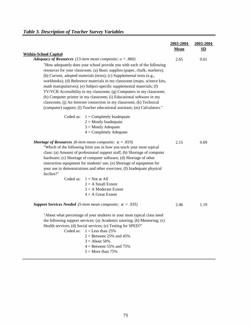
the five years of unitary status, it is also true the rezoning one cluster (or even one school)

sent ripple effects throughout the district that affected several school zones in smaller

ways. Most schools experience a one-time large change in zoning patterns, but most

schools also experience mild rezoning throughout the six years of the study; therefore,

school attendance zones tend to change every year of the study, and these changes are

captivated in my census-based measures of schools’ neighborhoods.

Disorganization theory identifies four important constructs to consider when

measuring neighborhood effects: residential stability, ethnic diversity, family disruption,

and socioeconomic conditions. All of these constructs are created from the variables

available for each BG in the 2000 census data. The variable values for each BG are

aggregated to the school zone level, thereby creating neighborhood context indicators that

essentially become school-level variables.

Residential stability. Residential stability measures the proportion of residents

who have lived in the same dwelling for at least five years. This is an important

neighborhood characteristic to consider because the assimilation of newcomers into a

neighborhood is a sequential process, and therefore residential mobility acts as a barrier

to the development of friendships and networks (see Weicher, 1990). Residential

stability, on the other hand, has a positive effect on social cohesion from increased

friendship networks and decreased anonymity among neighbors. In fact, regardless of

their own length of residence, residents who live in high-turnover neighborhoods have

fewer opportunities to form friendships and organizational contacts. They tend to be less

satisfied with their communities, and may be less motivated to form friendships

(Sampson, 1991). I expect residential stability to enhance processes related to collective

70

socialization and social networks and, in turn, improve educational outcomes of students

attending neighborhood schools.

Ethnic diversity. To capture the neighborhood’s level of racial and ethnic

diversity, I subtract from one the sum of the squared proportions of Whites, African

Americans, Asians, Native Americans, and others (see Bellair, 1997; Sampson & Groves,

1989; and Warner & Rountree, 1997). This measure theoretically rages from 0 to .8, with

high scores indicating a neighborhood that is racially and ethnically heterogeneous and

low scores indicating a neighborhood that is racially and ethnically homogeneous.

Diversity is measured in such a way because of the theoretical expectation that

racial/ethnic heterogeneity keeps inner-city residents from forming consensus about

norms and values (Elliot, Wilson, Huizinga, Sampson, Elliot, & Rankin, 1996; Sampson

& Groves, 1989; Shaw & McKay, 1942).

Family disruption. Sampson (1985) suggests that single parenthood strains

resources of time, money, and energy—all of which interfere with parents’ ability to

supervise their children and communicate with other adults in the neighborhood.

Family disruption is the proportion of children age 18 and younger living in single-parent

families.

Socioeconomic conditions. The “socioeconomic conditions” concept is divided

into two constructs: “social advantage” and “economic deprivation.” Social advantage is

a mean composite of the proportion of college graduates among adults who are at least 25

years of age and the proportion of employed persons with professional or managerial

occupations (α = .972). This factor allows me to consider the spatial concentration of

“advantage” in terms of the potential pool of positive role models in the neighborhood

71

(Morenoff & Tienda, 1997). Similarly, economic deprivation is also a mean composite

of two items. It includes the proportion of residents over age 16 who are unemployed or

not in the labor force as well as the proportion of individuals with incomes below the

poverty level (α = .854). I include the jobless rate because Wilson (1996) has

emphasized its role in the creation of “the new urban poverty.” Joining measures of

unemployment and poverty allows me to take into consideration an additional dimension

of material deprivation (see Ainsworth, 2002).

Mediating Variable

The most common strategy in studying neighborhood effects is to estimate a

direct effects model where several variables are entered as controls alongside certain

neighborhood characteristics. However, Sampson, Morenoff, and Gannon-Rowley

(2002) argue that this strategy confounds the importance of other community influences

such as school climate, etc. “Static models that estimate the direct effect of current

neighborhood context on a particular outcome (e.g., delinquency, level of academic

achievement) may be partitioning out relevant variable in a host of mediating and

developmental pathways of influence” (p. 469). This is a call for tests of indirect

pathways that may mediate the effects of neighborhood contexts. As is discussed in the

review of literature, it is hypothesized that schools may, at least partially, mediate the

relationship between neighborhood characteristics and student outcomes (Ainsworth,

2002). This idea is fueled by the research indicating that place matters in educational

environments and that schools can act as a stabilizing force in neighborhoods (Driscoll,

2001; Morris, 2001).

72

In response to the need to explore avenues of mediation when studying

neighborhood contexts, I test whether or not neighborhood characteristics are mediated

by enhanced option schools. The district data, however, offers very little data on the

characteristics of enhanced option school. It does include a school type indicator. That

is, we know which schools are zoned schools and which are specified as enhanced option

schools in each year of the study. Enhanced option schools were designed to be “the

most effective elementary program necessary for high risk student to have early and

sustained success in school” (Greensville Metropolitan Public Schools, n.d., p. 1). “The

purpose of Enhanced Options Schools is to provide education, health, social, and

recreational services to students, families, and the community that ensures student

success now and in the future” (Greensville Metropolitan Public Schools, n.d., p. 2).

These schools were clearly established with the purpose of mediating the negative effects

of living in impoverished communities on student outcomes. Enhanced option schools

are placed in inner-city neighborhoods to “provide a neighborhood school option for

parents of inner city young children—the group who had traditionally bore the burden of

court ordered busing” (Greensville Metropolitan Public Schools, n.d., p. 1).

Given the purpose and history of enhanced option schools, a simple school type

indicator (1 = school is an enhanced option school, and 0 = school is a regular zoned

school) is sufficient to detect the possible mediating effect of schools. Thus, this

dichotomous school type measure is used for two purposes: first, to test whether or not

attending an enhanced option school influences students’ participation and engagement;

and second, to test whether or not enhanced option schools are able to mediate the

neighborhood effects that influence the same student outcomes.

73

This measure, however, is not without weaknesses. Should an enhanced option

effect emerge, the reason for the effect would probably be less clear than would be

desirable. To explore this further, I use the schools surveyed as part of the teacher survey

to assess descriptively the differences between enhanced option schools and regular

zoned schools.

School Characteristics Constructs from the Greensville Teacher Survey

The district-wide data does not contain contextual measures of school

characteristics. This is somewhat problematic because if enhanced option schools are

found to have an effect on student outcomes, the characteristics of enhanced option

schools that are most influential on student outcomes will be unknown. The teacher

surveys provide contextualized measures of school characteristics (teacher responses

aggregated to the school level). The aggregate measures calculated from the teacher

survey include composites of the following variables: within-school capital (such as

adequacy of resources, shortage or resources, support services needed, and support

services received); academic climate (academic press); environmental climate

(professional climate, institutional challenges, and lack of student engagement); and

social networks (such as school and community partnering, barriers to parent

involvement, and communication with parents) (see Table 3).

Within-school capital. Four constructs are used to measure within-school capital:

adequacy of resources (a 13-item mean composite; α = .860); shortage of resources (a 6-

item mean composite; α = .819); support serviced needed (a 5-item mean composite; α =

.935); and support services received (a 5-item mean composite; α = .926). To assess

74

2003-2004 Mean

2003-2004 SD

Within-School CapitalAdequacy of Resources (13-item mean composite; α = .860) 2.65 0.61

Coded as: 1 = Completely Inadequate2 = Mostly Inadequate3 = Mostly Adequate4 = Completely Adequate

Shortage of Resources (6-item mean composite; " = .819) 2.15 0.69

Coded as: 1 = Not at All2 = A Small Extent3 = A Moderate Extent4 = A Great Extent

Support Services Needed (5-item mean composite; " = .935) 2.46 1.19

Coded as: 1 = Less than 25%2 = Between 25% and 45%3 = About 50%4 = Between 55% and 75%5 = More than 75%

"About what percentage of your students in your most typical class need the following support services: (a) Academic tutoring; (b) Mentoring; (c) Health services; (d) Social services; (e) Testing for SPED?"

Table 3. Description of Teacher Survey Variables

"How adequately does your school provide you with each of the following resources for your classroom: (a) Basic supplies (paper, chalk, markers); (b) Current, adopted materials (texts); (c) Supplemental texts (e.g., workbooks); (d) Reference materials in my classroom (maps, science kits, math manipulatives); (e) Subject-specific supplemental materials; (f) TV/VCR Accessibility in my classroom; (g) Computers in my classroom; (h) Computer printer in my classroom; (i) Educational software in my classroom; (j) An Internet connection in my classroom; (k) Technical (computer) support; (l) Teacher educational assistant; (m) Calculators."

"Which of the following limit you in how you teach your most typical class: (a) Amount of professional support staff; (b) Shortage of computer hardware; (c) Shortage of computer software; (d) Shortage of other instruction equipment for students' use; (e) Shortage of equipment for your use in demonstrations and other exercises; (f) Inadequate physical facilies?"

75

Within-School Capital (continued)

Support Services Received (5-item mean composite; " = .926) 2.25 1.31

Coded as: 1 = Less than 25%2 = Between 25% and 45%3 = About 50%4 = Between 55% and 75%5 = More than 75%

Academic ClimateAcademic Press (7-item mean composite; " = .739) 3.14 0.59

Coded as: 1 = Almost None2 = Some3 = Most4 = Nearly All

Environmental ClimateProfessional Climate (11-item mean composite; " = .888) 2.97 0.50

Coded as: 1 = Strongly Disagree2 = Disagree3 = Agree4 = Strongly Agree

"About what percentage of your students in your most typical class who need the following support services actually receive them: (a) Academic tutoring; (b) Mentoring; (c) Health services; (d) Social services; (e) Testing for SPED?"

Table 3 (continued). Description of Teacher Survey Variables

"How many teachers at this school: (a) Feel responsible when students fail; (b) Feel responsible to help each other do their best; (c) Help maintain discipline in the entire school, not just their classroom; (d) Take responsibility for improving the school; (e) Feel responsible for helping students develop self-control; (f) Set high standards for their own performance; (g) Feel responsible that all students learn?"

Teachers were asked to mark the extent to which they agreed or disagreed with each of the following statements about the teachers in their school: (a) Most teachers are continually learning and seeking new ideas; (b) Most teachers make a conscious effort to coordinate their teaching with instruction at other grade levels; (c) Most teachers are supported in their efforts to experiment and develop new programs and curricula; (d) When teachers are not doing a good job, the principal works with then to improve instruction; (e) Performance evaluation procedures in this school help teachers grow professionally; (f) My principal is available when I need to see him/her; (g) Other teachers encourage me to try out new ideas; (h) Teachers receive the help they need from the principal when problems arise; (i) The principal spends time in my classroom observing my teaching and provides feedback; (j) In-service training and staff development programs in this school help teachers grow professionally; (k) The staff is continually evaluating its programs and activities.

76

Institutional Challenges (7-item mean composite; " = .753) 2.12 0.61

Coded as: 1 = Not at All2 = A Small Extent3 = A Moderate Extent4 = A Great Extent

Lack of Student Engagement (4-item mean composite; " = .829) 2.53 0.78

Coded as: 1 = Not at All2 = A Small Extent3 = A Moderate Extent4 = A Great Extent

Social NetworksSchool & Community Partnering (7-item mean composite; " = .739) 1.50 0.62

Coded as: 0 = Never1 = A Few Time a Year2 = Once or Twice a Month3 = Once or Twice a Week4 = Almost Daily

Barriers to Parent Involvement (5-item mean composite; " = .663) 2.28 0.57

Coded as: 1 = Never2 = Rarely3 = Sometimes4 = Often

"Indicate how much each of the following limit you in how you teach your most typical class: (a) Low morale among fellow teachers/administrators; (b) Students who come from a wide range of backgrounds; (c) Threat(s) to personal safety or safety of students; (d) The noise level in the school building; (e) Students with special needs (e.g., hearing, vision, speech, impairment, physical disabilities, mental or emotional/psychological impairment); (f) High student/teacher ratio; (g) Students with different academic abilities."

"This school year, how often have you: (a) Brought in a guest speaker form the school’s community; (b) Talked with students about people and/or events in the community; (c) Consulted with members of the community to better understand your students; (d) Taken students on a field trip to a local site or organization; (e) Talked with students about their cultures; (f) Talked with students about their lives at home?"

"How often do each of the following affect parent involvement at this school: (a) The distance parents have to travel from their home to the school is too far; (b) Parents do not feel welcome at this school; (c) Parents’ work schedules conflict with meeting and conference times at the school; (d) Lack of transportation for children; (e) Lack of childcare?"

"Which of the following limit you in how you teach your most typical class: (a) Uninterested students; (b) Disruptive students; (c) Parents uninterested in their children’s learning progress; (d) Low morale among students."

Table 3 (continued). Description of Teacher Survey Variables

77

Social Networks (continued)Teacher Communication with Parents (5-item mean composite; " = .847) 3.05 0.68

Coded as: 1 = Never2 = Sometimes3 = Usually4 = Always

Means and Standard Deviations are reported for Zoned Schools and Enhanced Option Schools combined for the 2003-2004 school year.

"Teachers may communicate many different types of information to their students’ families. How often do you communicate the following information to parents of your students? (a) Inform parents about learning objectives in core academic subjects; (b) Contact parents when their child Is encountering academic problems; (c) Provide parents with examples of excellent student work; (d) Provide parents with specific activities for children and parents to do to improve students’ grades; (e) Assign homework that requires children to interact with parents?"

Table 3 (continued). Description of Teacher Survey Variables

N = 164 Teacher in 5 Enhanced Option Schools & 325 Teachers in 12 Zoned Schools.

78

teachers perceptions of the adequacy of school resources, teachers were asked to respond

to the following question: “How adequately does your school provide you with each of

the following resources for your classroom: (a) Basic supplies (paper, chalk, markers);

(b) Current, adopted materials (texts); (c) Supplemental texts (e.g., workbooks); (d)

Reference materials in my classroom (maps, science kits, math manipulatives); (e)

Subject-specific supplemental materials; (f) TV/VCR Accessibility in my classroom; (g)

Computers in my classroom; (h) Computer printer in my classroom; (i) Educational

software in my classroom; (j) An Internet connection in my classroom; (k) Technical

(computer) support; (l) Teacher educational assistant; (m) Calculators.” Teachers rated

the adequacy of each resources as 1 = Completely inadequate, 2 = Mostly inadequate, 3 =

Mostly adequate, or 4 = Completely adequate.

Teachers were also asked to assess the extent to which they experienced shortages

of resources in their classrooms. They were asked: “Which of the following limit you in

how you reach your most typical class: (a) Amount of professional staff; (b) Shortage of

computer hardware; (c) Shortage of computer software; (d) Shortage of other instruction

equipment for students’ use; (e) Shortage of equipment for your use in demonstrations

and other exercises; and (f) Inadequate physical facilities.” Response categories were 1 =

Not at all, 2 = A small extent, 3 = A moderate extent, and 4 = A great extent.

The support services needed composite was created from the following question:

“About what percentage of your students in your most typical class need the following

support services: (a) Academic tutoring; (b) Mentoring; (c) Health services; (d) Social

services; (e) Testing for SPED? 1 = Less than 25%, 2 = 25% to 45%, 3 = About 50%, 4

= 55% to 75%, or 5 = More than 75%.”

79

Similarly, the support serviced received composite measures teachers responses to

the following questions: “About what percentage of your students in your most typical

class who need the following support services actually receive them: (a) Academic

tutoring; (b) Mentoring; (c) Health services; (d) Social services; (e) Testing for SPED? 1

= Less than 25%, 2 = 25% to 45%, 3 = About 50%, 4 = 55% to 75%, or 5 = More than

75%.”

Academic climate. Academic climate is measured with one composite aimed at

assessing the school’s academic press. Teachers were asked, “How many teachers at this

school: (a) Feel responsible when students fail; (b) Feel responsible to help each other do

their best; (c) Help maintain discipline in the entire school, not just their classroom; (d)

Take responsibility for improving the school; (e) Feel responsible for helping students

develop self-control; (f) Set high standards for their own performance; (g) Feel

responsible that all students learn? 1 = Almost none, 2 = Some, 3 = Most, or 4 = Nearly

all.” The 7-item mean composite has an alpha reliability of α = .739.

Environmental climate. Professional climate, institutional challenges, and student

engagement are all considered part of a school’s environmental climate and may be

important school characteristics that could mediate the effects of neighborhoods on

student outcomes. Professional climate, an 11-item mean composite with an alpha

reliability of α = .888, assess how teachers feel about other teachers and professionals in

their school. Teachers were asked to mark the extent to which they agreed or disagreed

with each of the following statements about the teachers in their school: “(a) Most

teachers are continually learning and seeking new ideas; (b) Most teachers make a

conscious effort to coordinate their teaching with instruction at other grade levels; (c)

80

Most teachers are supported in their efforts to experiment and develop new programs and

curricula; (d) When teachers are not doing a good job, the principal works with then to

improve instruction; (e) Performance evaluation procedures in this school help teachers

grow professionally; (f) My principal is available when I need to see him/her; (g) Other

teachers encourage me to try out new ideas; (h) Teachers receive the help they need from

the principal when problems arise; (i) The principal spends time in my classroom

observing my teaching and provides feedback; (j) In-service training and staff

development programs in this school help teachers grow professionally; (k) The staff is

continually evaluating its programs and activities.” The response options were 1 =

Strongly disagree, 2 = Disagree, 3 = Agree, and 4 = Strongly agree.

A composite assessing institutional challenges was also created from the

following 7 items. Teachers were asked, indicate how much each of the following limit

them in how they teach their most typical class: “(a) Low morale among fellow

teachers/administrators; (b) Students who come from a wide range of backgrounds; (c)

Threat(s) to personal safety or safety of students; (d) The noise level in the school

building; (e) Students with special needs (e.g., hearing, vision, speech, impairment,

physical disabilities, mental or emotional/psychological impairment); (f) High

student/teacher ratio; (g) Students with different academic abilities.” Response

categories were 1 = Not at all, 2 = Small extent, 3 = Moderate extent, or 4 = Great extent.

The composite measure was reliable at the α = .753 level.

Questions regarding student engagement (or a lack thereof) were also asked, from

which a 4-item mean composite was formed. Teachers were asked, “Which of the

following limit you in how you teach your most typical class: (a) Uninterested students;

81

(b) Disruptive students; (c) Parents uninterested in their children’s learning progress; (d)

Low morale among students.” Responses include: 1 = Not at all, 2 = Small extent, 3 =

Moderate extent, and 4 = Great extent (α = .829).

Social networks. The final concept measured in the teacher survey, social

networks, is assessed through three composite measures: school and community

partnering, barriers to parent involvement, and communication with parents. The school

and community partnering composite (α = .739) was created from 7 items. Teachers

were asked, “This school year, how often have you: (a) Brought in a guest speaker form

the school’s community; (b) Talked with students about people and/or events in the

community; (c) Consulted with members of the community to better understand your

students; (d) Taken students on a field trip to a local site or organization; (e) Talked with

students about their cultures; (f) Talked with students about their lives at home?”

Teacher responses include 0 = Never, 1 = A few times a year, 2 = Once or twice a month,

3 = Once or twice a week, or 4 = Almost daily.

Barriers to parent involvement is another important measure, and one the district

hoped limit as they moved to a system of neighborhood schools. In theory, barriers

should be few in number. To assess this empirically, teachers responded to the following

question: “How often do each of the following affect parent involvement at this school:

(a) The distance parents have to travel from their home to the school is too far; (b)

Parents do not feel welcome at this school; (c) Parents’ work schedules conflict with

meeting and conference times at the school; (d) Lack of transportation for children; (e)

Lack of childcare?” Teachers answered with 1 = Never, 2 = Rarely, 3 = Sometimes, or 4

82

= Often. Responses to these five items were averaged to create a composite measure of

barriers to parent involvement (α = .663).

The final composite measure of social networks is communication with parents.

Teachers were asked the following question: “Teachers may communicate many different

types of information to their students’ families. How often do you communicate the

following information to parents of your students? (a) Inform parents about learning

objectives in core academic subjects; (b) Contact parents when their child Is encountering

academic problems; (c) Provide parents with examples of excellent student work; (d)

Provide parents with specific activities for children and parents to do to improve

students’ grades; (e) Assign homework that requires children to interact with parents?”

Teachers gave answers of 1 = Never, 2 = Sometimes, 3 = Usually, and 4 = Always. The

measure in reliable at the α = .847 level.

Analyses

Three sets of analyses are used to explore the context of this study and to address

the research questions. First, I use descriptive analyses to track district-wide changes on

the outcome measures, attendance and disciplinary events, as well as changes in schools

and school zones over time. Second, to address the extent to which student outcomes are

predicted by the characteristics of school neighborhoods and to determine whether or not

these neighborhood effects can be mediated by schools with enhanced options, I apply

cross-classified growth models (HCM) that include all six years of district-level data.

The HCM analyses mark those which are most critical to this study and most

instrumental in addressing the research questions outlined in this study. Third, to further

83

address the differences between enhanced option schools and regular zoned schools I use

the teacher survey data to assess descriptive differences between enhanced option school

characteristics and the characteristics of regular zoned schools. Results from these

descriptive analyses are used to interpret the findings from the HCM analyses.

Cross-Classified Growth Models

The longitudinal nature of the data available from the district allows for the

tracking of students and their experiences over time. This type of modeling permits the

assessment of whether or not student- and school- level variables are more or less

predictive of student attendance and discipline over time. Additionally, data are

hierarchical, meaning that students are nested within schools over time. Because student

observations are not truly independent of one another when dealing with nested

hierarchies, students who share the same school are likely to experience some shared

variance. Multilevel growth models adjust for this non-independence of observations.

However, a traditional hierarchical linear model (HLM) model is insufficient in making

use of this type of longitudinal data where students change schools over time. HLM

growth modeling is a useful modeling approach when lower-level units are nested within

one and only one higher-level unit. In these data, however, students do not belong to one

and only one school; therefore, the nesting structure of the data is more complex in which

individual, time-varying student observations are cross-classified by time-invariant

student characteristics and schools. Cross-classified growth models (HCM) are ideal for

such data structures (Raudenbush & Bryk, 2002). Another advantage to growth modeling

using the HCM framework is that it is not necessary for each student in the analyses to

84

have the same number of waves of data. All cases can be used, even if a student is only

observed at one point in time (Singer & Willett, 2003).

Level-1 of the HCMs used in this study includes all student-level time-variant

measures and a growth trajectory. These student-level measures are the dependent

variables as well as the series of dummy variables used to control for student grade.

Time-varying student observations are cross-classified by Row-level indicators and

Column-level indicators. Row-level indicators consist of the following student time-

invariant measures: student race, gender, poverty status, IEP status, and LEP status (see

Appendix C, Equations 1.1 and 1.2 for).

Column-level indicators refer to all school-level measures. The traditional HCM

framework is somewhat problematic for this study in that it assumes that all Row- and

Column-level measures are time-invariant. In this study, however, school-level measures

are quite dynamic over the six years of the study. This problem is resolved by assigning

each school a unique identification number of every year it appears in the study. This

maintains the nesting structure of students within schools, but allows students to

experience different school characteristics over the course of the study. Thus, student

observations (at level-1) are nested within students which are nested within school

observations, where students are nested within a different school observation in each year

of the study.

I estimate three stepwise models for each dependent variable. The first step

models the dependent variables as a function of neighborhood characteristics. In the

second step, all other school- and student-level control variables are included in the

model. And finally, the third step adds the mediating variable of whether or not a school

85

is an enhanced option school. This stepwise approach to estimating these models is

functional in terms of addressing some of the methodological issues that are discussed

below.

Methodological Considerations

Three methodological considerations are addressed at the outset. I first discuss

the treatment of non-normal distributions of my dependent variables, after which I

discuss the method I employ for detecting mediated relationships between variables, and

finally, I discuss sources of bias inherent in this study and how they are dealt with.

Distribution of dependent variables. Traditional regression assumes a certain

distribution for dependent variables. Dependent variables should be normally distributed

with a symmetric distribution of errors and constant variance (Cohen, Cohen, West, &

Aiken, 2003). Neither of my dependent variables—number of absences and number of

disciplinary events—meet these assumptions. However, because both of my dependent

variables are counts of the occurrence of rare events, they seem to follow the pattern of a

Poisson distribution. The three main requirements for a Poisson distribution are (a) the

distribution is skewed; (b) the distribution is non-negative; and (c) the variance increases

as the mean increases (Gardner, Mulvey, & Shaw, 1995). Table 4 reports descriptive

statistics for each of the dependent variables for each year of the study. These descriptive

statistics include skewness and Kurtosis statistics. The positive skewness statistic for

each of the dependent variables across all years of the study indicates a non-normal

distribution with a long right tail. Similarly, the Kurtosis statistic indicates that the

observations cluster more and have longer tails than those in a normal distribution. Both

86

Table 4. Distribution of Dependent Variables

1998-1999 1999-2000 2000-2001 2001-2002 2002-2003 2003-2004 All YearsDependant Variables

Number of AbsencesMinimum 0 0 0 0 0 0 0Maximum 134 136 169 136 140 137 169Mean 8.25 8.02 7.86 7.74 8.13 8.15 8.02Standard Deviation 8.80 8.87 8.65 7.88 8.04 7.80 8.38Skewness 3.17 3.35 3.54 2.84 2.84 2.36 3.07Kurtosis 17.84 20.38 26.60 16.51 16.84 10.78 18.92N 28641 28752 29160 29587 28787 28859 173786

Number of Disciplinary EventsMinimum 0 0 0 0 0 0 0Maximum 37 45 37 44 48 32 48Mean 0.83 0.82 0.79 0.84 0.94 1.05 0.88Standard Deviation 2.44 2.39 2.10 2.33 2.65 2.78 2.46Skewness 5.18 5.60 4.60 5.26 5.01 4.45 5.06Kurtosis 36.06 45.19 29.28 40.80 35.72 25.47 35.85N 29311 29459 29301 29623 28808 28890 175292

N = 171,030 Observations of 67,833 Students & 548 Observations of 104 Schools (over a 6-year period).

87

measures indicate that the dependent variables follow a Poisson distribution. Poisson

regression is a generalized linear model that uses a log transformation to adjust for the

skewness and prevents the model from producing negative predicted values. Poisson

regression also models the variance as a function of the mean (Gardner, Mulvey, &

Shaw, 1995). Additionally, the two outcome measures used in my analyses have

unbounded positive ranges, and the sample variance for both measures exceeds the mean

(see Table 4). In these cases, the observations are overdispersed with respect to a

traditional Poisson distribution. Therefore, an overdispersed Poisson regression within

the HCM framework is the modeling strategy employed to examine the effects of

neighborhoods and schools on absenteeism and number of disciplinary events.

Determining mediation. The criteria for establishing mediation are nicely

summarized by Howell (2002). First, the dependent variable(s) (absenteeism and

discipline, in this study) must be correlated with the independent variable that may be

mediated by some other variable. In this study, the independent variables of interest are

the characteristics of schools’ neighborhoods. Second, the independent variables must be

correlated with the mediating variable (in this case, whether or not the school is an

enhanced option school). Third, the mediating variable must be correlated with the

dependent variable, holding constant any direct effect of the independent variable on the

outcome variable(s). Complete mediation is established when the independent variable is

no longer correlated with the dependent variable when the mediating variable is entered

in the regression equation. Partial mediation occurs when the correlation between the

independent variable on the dependent variable is reduced when the mediating variable is

added.

88

Specific to the study at hand, all variables are entered into the HCM model with

the exception of the mediating variable. After estimating a model without the mediating

variable, the mediator is included in the model and the two sets of results for the

independent variables of interest are compared (Baron & Kenny, 1986). In this case, if

enhanced option schools completely mediate the effects of the schools’ neighborhood,

any significant findings in the model without the mediator will no longer be significant

when the mediating variable is included. In the case of partial mediation, the effect of the

neighborhood variables will be closer to zero, yet still significant when the mediating

variable is added.

Sources of bias. I am primarily concerned with three possible sources of bias in

my analyses, each of which represents a typical problem when studying the effects of

neighborhoods on individuals. Measurement error contributes to two possible sources of

bias. First, error is associated with the creation of the neighborhood context variables,

and second, the lack of ideal measures at the student level could contribute to omitted

variable bias. The third issue is that of highly correlated independent variables. Each of

these issues is addressed more thoroughly in the following paragraphs.

Crane (1991) suggests that possibly the largest source of measurement error when

measuring neighborhood effects is introduced when defining the neighborhoods

themselves. Most studies use census data and census boundaries to define

neighborhoods; however, these boundaries offer imperfect, and often overlapping

operational definitions of neighborhoods. This aggravates the problem of measurement

error. Crane (1991) states: “There is one saving grace, however. The bias that

measurement error generates is unambiguously downward (i.e., toward zero), thus

89

making estimates of neighborhood effects conservative” (p. 1246). Because there are

overlaps between true boundaries and operational boundaries, operationally defined

neighborhoods are weighted averaged of actual separate neighborhoods. This adds an

element of randomness to the measured association between neighborhood characteristics

and the dependent variables. Thus, the fact that I define neighborhoods as school zones

may introduce bias, but the bias is likely to underestimate the effects of neighborhoods.

Omitted variable bias is another problem inherent in my analyses. The literature

on neighborhood effects has been criticized because of the absence of data combining

information at the individual and neighborhood level (Brooks-Gunn, Duncan, Klebanov,

& Sealand, 1993; Mayer & Jencks, 1989). Ideally, I would be able to control for the

contexts of students’ residential neighborhoods while estimating the effects of those same

neighborhood characteristics as they are aggregated to the school zone level.

Unfortunately, the Greensville school district data does not provide the necessary student

identifiers such as address and zip codes.13 I am able to control for student race and

eligibility for free and reduced lunch, which may be reasonable proxies for students’

home environments and neighborhoods. But it is possible that the social characteristics

of the block group a student lives in is more important than the social characteristics of

their school attendance zone. To the extent that this is true, the omission of student-level

measures of neighborhood characteristics may bias my estimates of neighborhood effects

13 Much of the neighborhood effects research uses individuals’ zip codes to compute measures of neighborhood contexts using the census. However, zip codes are quite variable in terms of the geographic area they include. For example, in the county that makes up the Metro school district) there are 467 census block groups (which are used in this study to compute the neighborhood contexts of school attendance zones). However, there are only 48 5-digit zip codes in the county (excluding 8 zip codes that are assigned to universities and federal government agencies that have their own post offices and their own zip codes). It is likely that measures of a student’s home neighborhood (based on their zip code, if it were accessible in this dataset) would be much less precise than the measures used here to indicate the social contexts of their school zone, given that school attendance zones in all years of the study are significantly smaller than areas defined by zip codes.

90

upward. Nevertheless, correlations between my measures of the social context of school

zones and the percent of students eligible for free and reduced lunch at the school were

highly correlated (see Table 5); therefore, student-level measures of race and whether or

not the student is eligible for free and reduced lunch may be an acceptable proxy for

student’s residential neighborhood. This assumption, however, is not testable with the

available data.

Regardless, other researchers identify the common practice in neighborhood

effects research of looking at the characteristics of individuals’ place of residence as

problematic (Sampson, Morenoff, & Gannon-Rowley, 2002). They argue that many

behaviors of interest take place in spaces outside of residential neighborhoods and that

many patterns of social interactions expand beyond residential neighborhoods. They

further suggest that examining residential neighborhoods is limiting and that, when using

neighborhood contexts to predict outcomes for children, neighborhood boundaries need

to be redefined in ways that are more consonant with social interactions of children’s

experiences (Sampson, Morenoff, & Gannon-Rowley, 2002). By defining neighborhoods

as school attendance zones, this study attempts to follow these recommendations. My

study addresses the effects of school neighborhoods on school-related outcomes;

therefore, it is possible that the most important unit of analysis—characteristics of school

zones—is predicted in the best way possible, regardless of my inability to control for

these same characteristics at the student level.

In addition to the measurement error inherent in this research, some of the

variables originally intended for my analyses are highly correlated. This too is a common

problem in the research on neighborhood effects (Mayer & Jencks, 1989). Specifically,

91

Table 5. Bivariate Correlations of School-Level Variables

Resid

entia

l Stab

ility

Ethn

ic Di

versi

tyFa

mily

Disr

uptio

nSo

cail

Adva

ntag

eEc

onom

ic De

priv

ation

% F

ree &

Red

uced

Lun

ch75

% fr

ee &

Red

uced

Lun

ch%

Afri

can A

mer

ican

75%

Afri

can A

mer

ican

Scho

ol S

ize

Teac

her T

urno

ver

Dista

nce

School Neighborhood CharacteristicsResidential Stability 1.000Ethnic Diversity of Neighborhood -0.253 1.000Family Disruption 0.065 0.082 1.000Socioeconomic Conditions Social Advantage -0.155 -0.444 -0.674 1.000 Economic Deprivation 0.009 -0.039 0.807 -0.566 1.000

School Characteristics% Free & Reduced Lunch 0.050 0.375 0.660 -0.737 0.624 1.00075% Free & Reduced Lunch or Greater (dichotomous) -0.031 0.241 0.577 -0.464 0.601 0.727 1.000% African American 0.088 0.417 0.601 -0.517 0.583 0.779 0.589 1.00075% African American or Greater (dichotomous) 0.196 0.076 0.472 -0.281 0.427 0.624 0.623 0.724 1.000School Size -0.308 0.252 -0.252 0.134 -0.313 -0.275 -0.240 -0.133 -0.242 1.000Teacher Turnover Rate -0.002 0.036 0.115 -0.108 0.090 0.201 0.154 0.233 0.222 -0.047 1.000Distance Between Home & School 0.145 -0.299 -0.450 0.427 -0.409 -0.452 -0.404 -0.280 -0.159 0.229 -0.032 1.000

N = 171,030 Observations of 67,833 Students & 548 Observations of 104 Schools (over a 6-year period).

92

the family disruption measure is highly correlated with the two indicators of

socioeconomic conditions, social advantage (Pearson’s r = -.674) and economic

deprivation (Pearson’s r = .807) (see Table 5). Because my measures of socioeconomic

conditions seem to be measuring essentially the same characteristic as the family

disruptions measure,14 family disruption is dropped from the HCM analyses.

Because schools of concentrated poverty are often racially isolated minority

schools in the Metro school district after unitary status, my measures of poverty and

racial composition of schools’ student bodies are also highly correlated. To address this

issue, I attempted to use a continuous poverty indicator and create a dichotomous

measure for racial isolation (1 = 75% minority or more; 0 = Less than 75% minority).

This, however, was unhelpful. The indicators are highly correlated regardless of how

they are constructed. Each of these indicators is also correlated with my economic

deprivation measure, which is expected given that “neighborhoods” in this study are

school-level measures. Therefore, these two school characteristics—school poverty and

racial mix—are omitted from HCM analyses. In this study, measures of school poverty

and the racial composition seem to be reflective of the neighborhood contexts from which

a school draws its population of students.

14 This is most likely due to the observance that single-parent families are likely to be living in poverty.

93

CHAPTER V

CHANGES IN SCHOOLS & SCHOOL ZONES OVER TIME

Before reporting the main results of this paper, it is first necessary to outline the

trends of the district over time. Several analyses are used to describe the changes that

took place in the district over the six-year span of time. First, I describe the average

values for each school-level variable and how they change across the six years of the

study. As part of my description of these changes over time, I run a basic 2-level HLM

growth model to determine whether or not the distance between schools and the

outermost perimeter of their attendance zones has changed significantly over time (see

Appendix C, Equations 2.1 and 2.2). This basic model includes only two variables, one

dependent variable (distance between home and school) and one independent variable

(growth over time). I use the six-year growth trajectory to predict distance between home

and school. The level-1 portion of the model includes 548 observations of schools nested

within 104 schools in the level-2 portion of the model. After describing the six-year

tends in the district, I run independent sample t-tests to assess the differences between

zoned schools and enhanced option schools across all years of the study. And finally, I

repeat these analyses comparing enhanced option schools to zoned schools with similar

demographic characteristics.

94

Changes in School Characteristics Over Time

Over the six-year period of unitary status, Metro Greensville has experienced

many changes in how education is organized and prioritized. Since the 1999 school

year—the first year of this study—the most notable difference is that enhanced option

schools have been implemented, and the number of them continues to grow (see Table 6).

In 2000 the district opened 2 enhanced option schools, and by 2004 they had added four

more. Regular zoned schools decreased in number from 93 in 1999 to 83 in 2004. This

seeming decrease in zoned schools does not represent school closures, rather a

transformation of zoned schools into other school types (such as magnet schools and

enhanced option schools). The number of schools district wide remained relatively stable

over the six-year course of this study—between 89 and 93 schools with student

attendance zones.

Zoned School Trends

From 1999 to 2004 zoned schools experience an increase in student who are

eligible for free and reduced lunch (see Table 6). In the base year of the study, an

average of 54% of the students in zoned schools was eligible. By 2004 61% of the

students in zoned schools, on average, were eligible. The district also experienced a

decrease in the percentage of white students. In 1999 47% of the students attending

zoned schools were white; however, by 2004 that percentage had dropped to 42%. Both

of these trends can be explained by the tendency for middle-class and upper-middle class

parents to consider other public school choice options, private schools, or leave the

district rather than send their children to a neighborhood school in Greensville. The

95

Table 6. Description of School-Level Changes Over Time

Zoned Schools

1998-1999 Average

1999-2000 Average

2000-2001 Average

2001-2002 Average

2002-2003 Average

2003-2004 Average

% Free & Reduced Lunch 53.75% 51.73% 53.74% 55.39% 58.88% 61.21%% White 46.62% 46.63% 45.02% 44.09% 42.40% 41.98%% African American 47.59% 46.03% 46.26% 45.25% 45.48% 44.57%% Other Races 5.79% 7.34% 8.72% 10.66% 12.12% 13.44%Teacher Turnover Rate 31.61% 18.07% 22.72% 27.25% 24.24% 29.06%School Size 489.47 491.78 492.00 505.59 507.64 506.03Number of Absences 7.66 7.32 7.12 7.06 7.46 7.27Number of Disciplinary Events 0.66 0.58 0.57 0.58 0.60 0.61Total N 93 91 91 87 85 83

Enhanced Option Schools

1998-1999 Average

1999-2000 Average

2000-2001 Average

2001-2002 Average

2002-2003 Average

2003-2004 Average

% Free & Reduced Lunch ― 89.44% 91.32% 88.58% 86.52% 91.68%% White ― 11.99% 5.17% 10.39% 8.91% 5.98%% African American ― 87.12% 94.16% 86.56% 88.80% 92.24%% Other Races ― 0.88% 0.68% 3.05% 2.29% 1.78%Teacher Turnover Rate ― 34.90% 16.98% 40.71% 22.35% 44.49%School Size ― 381.50 395.00 354.20 346.40 316.29Number of Absences ― 7.38 5.28 6.72 6.42 6.32Number of Disciplinary Events ― 0.30 0.67 0.23 0.44 0.48Total N 0 2 3 5 5 6

All Schools*

1998-1999 Average

1999-2000 Average

2000-2001 Average

2001-2002 Average

2002-2003 Average

2003-2004 Average

% Free & Reduced Lunch 53.75% 52.54% 54.94% 57.18% 60.40% 63.51%% White 46.62% 45.88% 43.74% 42.28% 40.56% 39.27%% African American 47.59% 46.92% 47.79% 47.47% 47.86% 48.16%% Other Races 5.79% 7.20% 8.47% 10.25% 11.58% 12.57%Teacher Turnover Rate 31.61% 18.43% 22.54% 27.97% 24.14% 30.22%School Size 489.47 489.41 488.90 497.45 498.78 491.75Number of Absences 7.66 7.32 7.06 7.04 7.40 7.19Number of Disciplinary Events 0.66 0.57 0.57 0.56 0.59 0.60Total N 93 93 94 92 90 89

* "All Schools" refers only to the schools with designated student attendance zones, which represents all schools used in this study.

96

percentage of African American students attending zoned schools also slight decreased

over the six years of the study. In 1999 48% of the students in zoned schools were

African American; however, by 2004 this percentage dropped by 2%. This trend can be

explained by the overwhelming presence and growth in the number of African American

students attending enhanced option schools, since the percentage of African Americans in

the district is fairly stable over time (about 48%). By contrast, zoned schools experience

an increase in the percentage of other races. In 1999 6% of zoned school students were

of other races, and by 2004 this percentage grew to 13%.

Interestingly, the teacher turnover rate in zoned schools was highest in 1999 at

32%. In 2000, the first year of unitary status, teacher turnover dropped by 14% and

steadily increased over the remaining years of the study. By 2004 teacher turnover had

climbed to 29%. School size has slightly but steadily increased over the six years of the

study. In 1999 an average of 489 students attended zoned schools. This number steadily

rose to 506 in 2004. The student outcomes of interest in this study remained fairly stable

over time; however, on average, both the number of absences and the number of

disciplinary events in zoned schools were highest in 1999. On average, students in zoned

schools were absent about 8 times in 1999 and were disciplined about .7 times in 1999.

In 2004 zoned school students were absent about 7 times and disciplined about .6 times.

Enhanced Option School Trends

Enhanced option schools follow a somewhat different trend over time (see Table

6). First, there is no real base-line for enhanced option schools. Because they were

introduced with the new SIP, enhanced option schools have always been neighborhood

97

schools. Between 2000 and 2004, the percentage of enhanced option students eligible for

free and reduced lunch increased slightly, from 89% to 92%. When compared to zoned

schools, enhanced option students are, on average, much more disadvantaged (by roughly

40% in every year of the study). In addition to the high concentrations of poverty,

enhanced option schools are also racially isolated. 87% of the students in enhanced

option schools in 2000 were African American, and by 2004 92% of enhanced option

students were African American. White students represented 12% of enhanced option

school student bodies in 2000, but this percentage decreased to 6% by 2004. Other races

have increased from 1% to 2% in enhanced options from 2000 to 2004.

Teacher turnover has increased over time and is quite high relative to the turnover

rate in zoned schools. In 2000, the teacher turnover rate for enhanced option schools was

35%. By 2004, this rate had climbed by 10%. In 2004, enhanced option schools

experienced a teacher turnover rate of 45%, compared to 29% in zoned schools. Even

though zoned schools in the district are becoming slightly larger, school size in enhanced

option schools has decreased over time. In 2000, enhanced option schools, on average,

served 382 students, and in 2004, the average school size was 316. Enhanced option

schools, on average, are smaller than zoned schools in all years; however, this

comparison in inappropriate given that all enhanced option schools are elementary

schools by design, and all elementary schools in the district are smaller than middle

schools. Similar to the trends in zoned schools, absenteeism in enhanced option schools

decreases over time. In 2000, enhanced option school students were, on average, absent

about 7 times per year. This number steadily declined to 6 times per year in 2004. As

mentioned earlier, zoned schools follow a similar trend; however, absenteeism is lower in

98

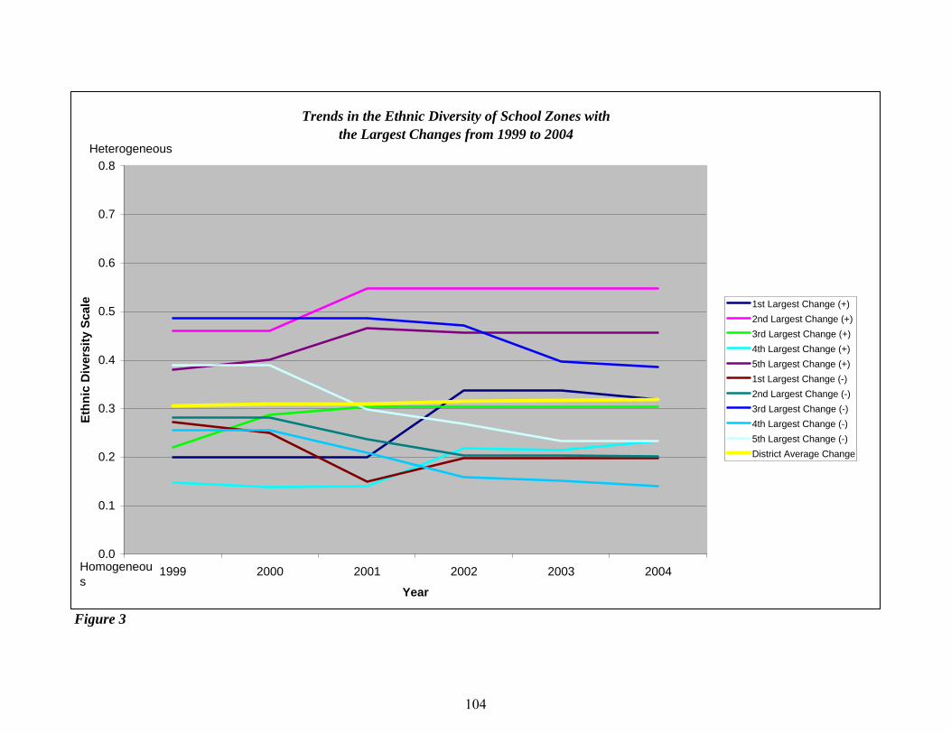
enhanced option schools in all years. Student discipline follows a different trend. In

2000, enhanced option students were disciplined about .3 times per year. This number

increased over the remaining five years, and in 2004, students were disciplined about .5

times per year. While the average number of disciplinary events is rising in enhanced

option schools, it did not reach the number of disciplinary events in zoned schools (.6 in

2004).

Changes in School Neighborhoods & School Zones over Time

In this study the characteristics of a school neighborhood is defined by the

geographic boundaries of the school attendance zone and how that attendance zone

overlaps with census block groups. Additionally all neighborhood context variables are

based on the 2000 census. Therefore, any changes in these measures represent changes in

school zones, and not changes in the geographic area. Each block group is assigned to at

least one school, and as such, district averages of these measures do not capture actual

changes in school zones by year. Change in the neighborhood context variables must be

assessed individually for each school (for an exhaustive list of changes in school zone

contexts by school, see Appendix D1 & Appendix D2). To describe these changes, I

report the range of changes experienced by school zones between 1999 and 2004 for each

of the five neighborhood characteristics used in this study.

Residential Stability

The district average for the residential stability of a school zone is 46%, with a

minimum of 23% and a maximum of 73%. This indicates that in the average school,

99

46% of the residents living within the school zone have lived at the same residence for at

least 5 years. Between the baseline year and 2004, schools in Metro experienced an

average change of -1.2% in residential stability (see Table 7). Twenty one school zones

(20%) did not experience any changes in residential stability; 46 schools (45%)

experienced a reduction in stability; and 37 schools (36%) experienced an increase in

residential stability. Of the school zones that became less stable over time, the most

dramatic change was a 14% decrease in stability, with an average change of -3%. Of the

school zones that became more stable over time, the most dramatic change was a 15%

increase in stability, with an average change of 4%. These changes indicate the type of

“polarization” that can be expected when a formerly desegregated school district returns

to closer-to-home schooling.

More school zones experience a decrease in residential stability over time;

however, many school zones experience a positive change in stability. The question then

becomes, which schools are changing the most? Are the schools that were most stable in

1999 becoming more or less stable? Figure 2 traces the changes in residential stability

over the six years of the study for 10 Metro schools. Five of these schools experienced

the greatest negative change in stability, and the other five experienced the greatest

positive change in stability. As is expected, the district average remains constant over

time at about 46%. Schools that experienced the highest rates of stability in 1999 tend to

become more stable over time. Likewise, schools that experience the lowest rates of

stability in 1999 tend to become less stable over time. Most of these schools are

clustered around the district average for residential stability in 1999; however, they are

more dispersed in 2004. Additionally, of these schools demonstrating the greatest

100

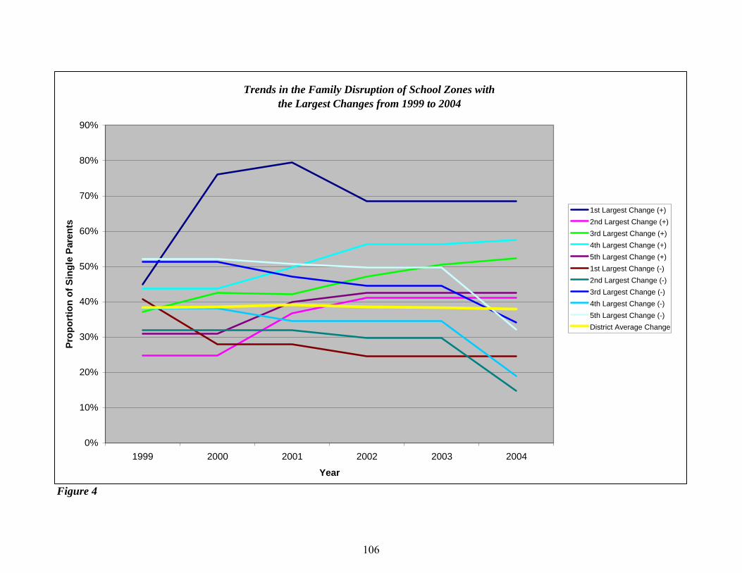
Table 7. Description of Change in the Contexts of School Zones over Time

Residential Stability Ethnic Diversity Family Disruption Social Advantage Economic Deprivation

District Minimum 23% 0.11 14% 12% 24%District Maximum 73% 0.55 85% 57% 62%District Average 46% 0.31 39% 28% 27%

Greatest Negative % Change -14% -16% -20% -21% -9%Greatest Positive % Change 15% 12% 32% 12% 16%Average % Change -1.2% 1.4% 0.3% 0.0% -1.0%Average Negative % Change -3.27% -3.97% -7.21% -3.40% -4.18%Average Positive % Change 4.05% 3.59% 6.67% 3.25% 3.90%

Number of Schools

% of Schools

Number of Schools

% of Schools

Number of Schools

% of Schools

Number of Schools

% of Schools

Number of Schools

% of Schools

-5% or Greater (negarive) 12 12% 11 11% 29 28% 7 7% 23 22%-1% to -4% Change 34 33% 25 24% 18 17% 28 27% 26 25%0% Change 21 20% 22 21% 18 17% 25 24% 24 23%1% to 4% Change 25 24% 35 34% 22 21% 33 32% 22 21%5% or Greater (positive) 12 12% 11 11% 17 16% 11 11% 9 9%

N 104 100% 104 100% 104 100% 104 100% 104 100%

Change is calculated by subtracting values from 2004 from the baseline values in 1999.

101

Trends in the Residential Stability of School Zones Experiencing the Largest Changes from 1999 to 2004

0%

10%

20%

30%

40%

50%

60%

70%

80%

1999 2000 2001 2002 2003 2004

Year

Prop

ortio

n of

Res

iden

ts L

ivin

g in

Sa

me

Dw

ellin

g fo

r 5 o

r Mor

e Ye

ars

1st Largest Change (+)

2nd Largest Change (+)

3rd Largest Change (+)

4th Largest Change (+)

5th Largest Change (+)

1st Largest Change (-)

2nd Largest Change (-)

3rd Largest Change (-)

4th Largest Change (-)

5th Largest Change (-)

District Average Change

Figure 2

102

changes over time, most of them fell below the district average for residential stability in

1999. Therefore, the schools with the greatest amount of change (both positive and

negative changes) tend to be schools that were lower than average in the base year.

Ethnic Diversity

Keeping in mind that ethnic diversity is measured on a 0 to .8 scale where 0

indicates complete homogeneity and .8 indicates complete heterogeneity, the district

average for the diversity school zones is .31, with a minimum of .11 and a maximum of

.55. Between the baseline year and 2004, schools in Metro experienced an average

change of 1.4% in ethnic diversity (see Table 7). Twenty two school zones (21%) did not

experience any changes in diversity; 36 schools (35%) experienced a reduction in

diversity; and 46 schools (45%) experienced an increase in ethnic diversity. Of the

school zones that became less diverse over time, the most dramatic change was a 16%

decrease in stability, with an average change of -4%. Of the school zones that became

more stable over time, the most dramatic change was a 12% increase in stability, with an

average change of 4%.

More school zones experience an increase in ethnic diversity over time; however,

the largest changes in ethnic diversity are negative. Figure 3 describes these changes

over time among the 10 most dynamic schools. Five of these schools experienced the

greatest negative change in diversity, and the other five experienced the greatest positive

change in diversity. Again, the district average remains constant over time at about .31.

Comparatively, four of these schools fall above the district average and six all below it in

1999. Unlike the trends for residential stability, these schools do not tend to be as tightly

103

Trends in the Ethnic Diversity of School Zones with the Largest Changes from 1999 to 2004

0.0

0.1

0.2

0.3

0.4

0.5

0.6

0.7

0.8

1999 2000 2001 2002 2003 2004

Year

Ethn

ic D

iver

sity

Sca

le 1st Largest Change (+)2nd Largest Change (+)3rd Largest Change (+)4th Largest Change (+)5th Largest Change (+)1st Largest Change (-)2nd Largest Change (-)3rd Largest Change (-)4th Largest Change (-)5th Largest Change (-)District Average Change

Heterogeneous

Homogeneous

Figure 3

104

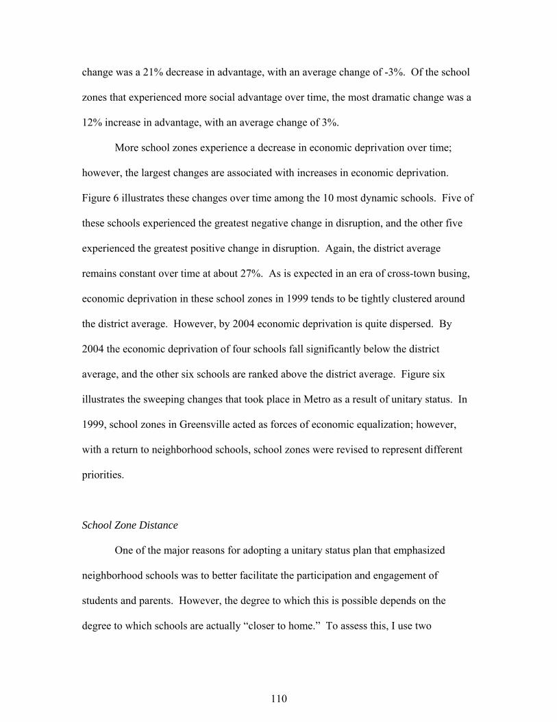
clustered around the district average in 1999. However, by 2004, diversity in these

school zones tends to be more dispersed. Once again, this provides evidence of

polarization as the district moves toward unitary status.

Family Disruption

The district average for the family disruption in a school zone is 39%, with a

minimum of 14% and a maximum of 85%. This indicates that in the average school,

39% of the children living within the school zone come from a single-parent home.

Between the baseline year and 2004, schools in Metro experienced an average change of

0.3% in family disruption (see Table 7). Eighteen school zones (17%) did not experience

any changes in disruption; 47 schools (45%) experienced a reduction in disruption; and

39 schools (37%) experienced an increase in family disruption. Of the school zones that

faced less family disruption over time, the most dramatic change was a 20% decrease in

disruption, with an average change of -7%. Of the school zones that faced more

disruption over time, the most dramatic change was a 32% increase in stability, with an

average change of 7%.

More school zones experience an increase in disruption over time; however, the

largest changes in disruption are negative. Figure 4 describes these changes over time

among the 10 most dynamic schools. Five of these schools experienced the greatest

negative change in disruption, and the other five experienced the greatest positive change

in disruption. Again, the district average remains constant over time at about 39%. Five

of these schools fall above the district average and five all below it in 1999. Unlike the

trends for residential stability and diversity, the trends for these schools are more clear in

105

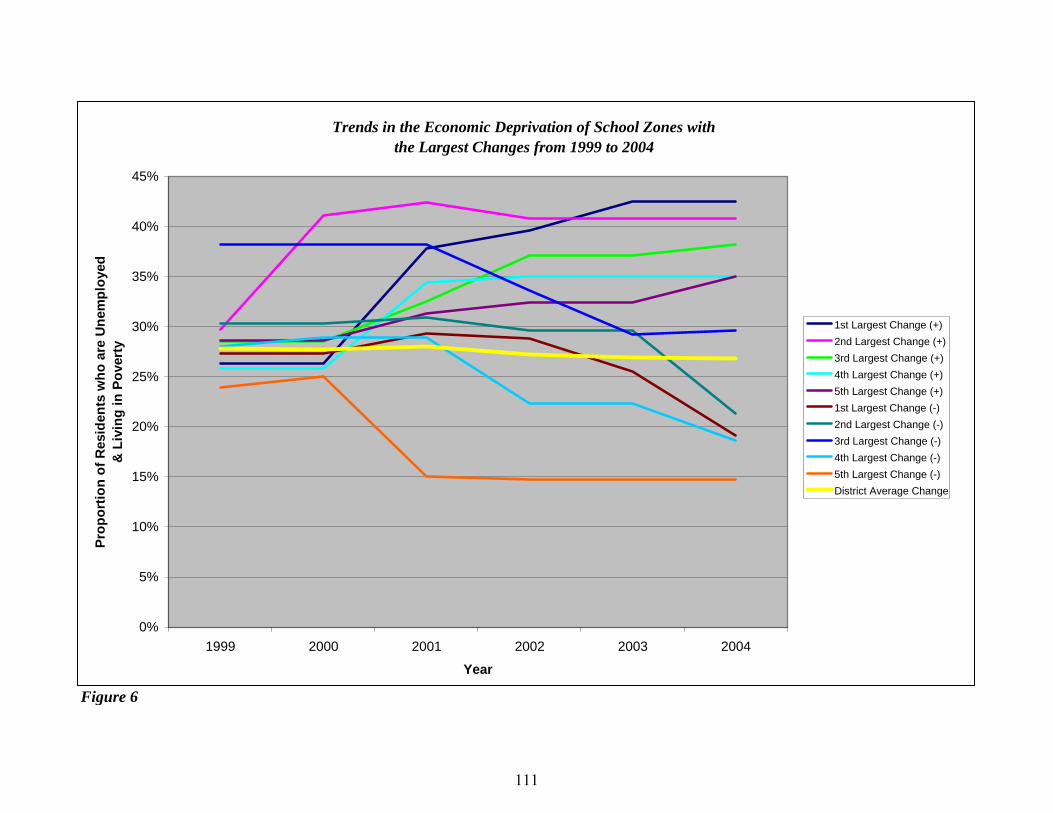
Trends in the Family Disruption of School Zones with the Largest Changes from 1999 to 2004

0%

10%

20%

30%

40%

50%

60%

70%

80%

90%

1999 2000 2001 2002 2003 2004

Year

Prop

ortio

n of

Sin

gle

Pare

nts

1st Largest Change (+)2nd Largest Change (+)3rd Largest Change (+)4th Largest Change (+)5th Largest Change (+)1st Largest Change (-)2nd Largest Change (-)3rd Largest Change (-)4th Largest Change (-)5th Largest Change (-)District Average Change

Figure 4

106

directionality. First, disruption in these school zones in 1999 tends to be more tightly

clustered around the district average in 1999 and more dispersed in 2004. Additionally,

most of the schools that fall above the district average in 1999 tend to experience a

decline in disruption, and most of the schools that fall above the district average in 1999

tend to experience an incline in disruption. Again, such trends are indicative of closer-to-

home schooling and the return to neighborhood schools.

Social Advantage

The district average for the social advantage in a school zone is 28%, with a

minimum of 12% and a maximum of 57%. This indicates that in the average school,

28% of residents have college degrees and/or professional employment (or both).

Between the baseline year and 2004, schools in Metro, on average, experienced a 0.1%

change in social advantage of the six years of the study (see Table 7). Twenty five school

zones (24%) did not experience any changes in social advantage; 35 schools (34%)

experienced a reduction in social advantage; and 44 schools (43%) experienced an

increase in social advantage. Of the school zones that faced less social advantage over

time, the most dramatic change was a 21% decrease in advantage, with an average

change of -3%. Of the school zones that experienced more social advantage over time,

the most dramatic change was a 12% increase in advantage, with an average change of

3%.

More school zones experience an increase in social advantage over time;

however, the largest changes are negative. Figure 5 illustrates these changes over time

among the 10 most dynamic schools. Five of these schools experienced the greatest

107

Trends in the Social Advantage of School Zones withthe Largest Changes from 1999 to 2004

0%

10%

20%

30%

40%

50%

60%

1999 2000 2001 2002 2003 2004

Year

Prop

ortio

n of

Res

iden

ts w

ith C

olle

ge D

egre

es

and

Prof

essi

onal

Em

ploy

men

t

1st Largest Change (+)2nd Largest Change (+)3rd Largest Change (+)4th Largest Change (+)5th Largest Change (+)1st Largest Change (-)2nd Largest Change (-)3rd Largest Change (-)4th Largest Change (-)5th Largest Change (-)District Average Change

Figure 5

108

negative change in disruption, and the other five experienced the greatest positive change

in disruption. Again, the district average remains constant over time at about 28%.

Social advantage in these school zones in 1999 tends to be dispersed; however, in 2004

social advantage is more polarized. Five schools that were ranked above the district

average in 1999 converged at a level of social advantage much higher than the district

average (about 43%) in 2004. In other words, school zones that experienced higher

levels of social advantage in 1999 tend to become more similar over time; however, they

remain socially advantaged when compared to the district average. However, the five

schools that were ranked closer to the district average or below the district average in

1999 tend to become less advantaged over time. The lowest ranking school on social

advantage in 1999, however, experienced an increase in social advantage over time.

These results are indicative of the district’s efforts to organize some school zones with

the intent of creating socioeconomic diversity among students.

Economic Deprivation

The district average for the economic deprivation in a school zone is 27%, with a

minimum of 24% and a maximum of 62%. This indicates that in the average school,

27% of residents are unemployed and/or living below the poverty line (or both).

Between the base year and 2004, schools in Metro, on average, experienced a -1%

change in economic deprivation (see Table 7). Twenty four school zones (23%) did not

experience any changes in deprivation; 49 schools (47%) experienced a reduction in

deprivation; and 31 schools (30%) experienced an increase in economic deprivation. Of

the school zones that faced less economic deprivation over time, the most dramatic

109

change was a 21% decrease in advantage, with an average change of -3%. Of the school

zones that experienced more social advantage over time, the most dramatic change was a

12% increase in advantage, with an average change of 3%.

More school zones experience a decrease in economic deprivation over time;

however, the largest changes are associated with increases in economic deprivation.

Figure 6 illustrates these changes over time among the 10 most dynamic schools. Five of

these schools experienced the greatest negative change in disruption, and the other five

experienced the greatest positive change in disruption. Again, the district average

remains constant over time at about 27%. As is expected in an era of cross-town busing,

economic deprivation in these school zones in 1999 tends to be tightly clustered around

the district average. However, by 2004 economic deprivation is quite dispersed. By

2004 the economic deprivation of four schools fall significantly below the district

average, and the other six schools are ranked above the district average. Figure six

illustrates the sweeping changes that took place in Metro as a result of unitary status. In

1999, school zones in Greensville acted as forces of economic equalization; however,

with a return to neighborhood schools, school zones were revised to represent different

priorities.

School Zone Distance

One of the major reasons for adopting a unitary status plan that emphasized

neighborhood schools was to better facilitate the participation and engagement of

students and parents. However, the degree to which this is possible depends on the

degree to which schools are actually “closer to home.” To assess this, I use two

110

Trends in the Economic Deprivation of School Zones withthe Largest Changes from 1999 to 2004

0%

5%

10%

15%

20%

25%

30%

35%

40%

45%

1999 2000 2001 2002 2003 2004

Year

Prop

ortio

n of

Res

iden

ts w

ho a

re U

nem

ploy

ed

& L

ivin

g in

Pov

erty

1st Largest Change (+)2nd Largest Change (+)3rd Largest Change (+)4th Largest Change (+)5th Largest Change (+)1st Largest Change (-)2nd Largest Change (-)3rd Largest Change (-)4th Largest Change (-)5th Largest Change (-)District Average Change

Figure 6

111

indicators of closer to home. First, as school zones change, they overlap with different

census block groups. In theory, as school zones are drawn to facilitate closeness to home,

the number of block groups a school zone comprises should be diminished. Secondly,

the radial distance between the school and the outermost perimeter of the school zone

should also be diminished.

The average school in Metro is made up of about 21 block groups, with a

minimum of 4 block groups and a maximum of 96 block groups. Between 1999 and

2004, schools in Metro, on average, experienced a -4 change in the number of block

groups in school zones (see Table 8). Thirteen schools (13%) did not experience any

changes in the number of block groups included within the zone; 57 schools (54%)

experienced a reduction in the number of block groups included in the zone; and 34

schools (33%) experienced an increase in the number of block groups included in within

the zone. Of the school zones that took in fewer block groups over time, the most

dramatic change was a decrease in the number of block groups by 30, with an average

reduction of 8. Of the schools that experienced an increase in the number of block

groups included within their zones, the most dramatic change was an increase in the

number of block groups by 32, with an average increase of 7. On average, more school

zones take in fewer block groups over time.

Another way to assess the change in “closeness to home” is to examine the

changes in the distance from the school to the outermost perimeter of the school zone.

The average school in Metro is 4.5 miles away from its outermost perimeter. The

smallest distance between home and school is .6 miles, and the greatest distance is about

12 miles. Between 1999 and 2004, schools in Metro, on average, experienced a -.5 mile

112

Table 8. Description of Change in the Number of Block Groups Associated with a School Zone over Time

Number of BGs in School Zone

District Minimum 4District Maximum 96District Average 21.02

Greatest Negative Change -30Greatest Positive Change 32Average Change in Change -3.74Average Negative Change in Change -8.46Average Positive Change in Change 7.18

Number of Schools % of SchoolsChange of -11 or Greater (negative) 15 14%Change of -1 to -10 42 40%0 Change 13 13%Change of 1 to 10 29 28%Change of 11 or Greater (positive) 5 5%

N 104 100%

Change is calculated by subtracting values from 2004 from the baseline values in 1999.

113

change in the distance between home and school15 (see Table 9). Sixteen schools (15%)

did not experience any changes in the distance between home and school; 53 schools

(51%) experienced a reduction in the distance between home and school; and 35 schools

(34%) experienced an increase in the distance between home and school. Of the school

zones that experienced a decrease in the distance between home and school over time, the

most dramatic change was a decrease in distance by 5.4 miles, with an average reduction

of 1.2 miles. Of the schools that experienced an increase in the distance between home

and school, the most dramatic change was an increase in distance by 2.8 miles, with an

average increase of .7 miles. Over the six year period addressed in this study, some

schools experienced an increase in the number of miles between home and school;

however, most schools experienced a reduction in the number of miles between home and

school. Thus, the distance between schools and the outermost perimeter of their

attendance zones has, for most schools, decreased over the six years of the study.

In addition to the descriptive analyses provided above that address the issue of

closer to home, I also use a multivariate approach to test whether or not the change in the

distance between home and school are significant. As was discussed previously, a 2-

level HLM growth model was used to assess this. Results indicate that indeed the

district’s rezoning efforts have resulted in school attendance zones that are significantly

closer to student’s homes (see Table 10). On average, the radial distance from schools to

the outermost perimeter of their attendance zones decreases by .11 miles per year (p <

.001). This represents a genuine shift in educational priorities. While some busing still

15 It is most appropriate to think of this measure as the radius of the school zone. It explicitly measures (in miles) the radial distance between a school and the outermost perimeter of its attendance zone. While this is a clear and accurate measure of the relative distance between home and school, it does not take into account conditions such as accessibility of roads and streets, traffic, and other such things that were thought to have influence the length and burden of bus rides during the desegregation era in Greensville.

114

Table 9. Description of Change in the Distance Between Home & School over Time

Distance Between Home & School

District Minimum 0.61 MilesDistrict Maximum 11.84 MilesDistrict Average 4.53 Miles

Greatest Negative Change in Miles -5.35Greatest Positive Change in Miles 2.79Average Change in Miles -0.52Average Negative Change in Miles -1.23Average Positive Change in Miles 0.73

Number of Schools % of Schools-1.1 Mile Change or Greater (negative) 22 21%-.01 to -1 Mile Change 31 30%0 Mile Change 16 15%.01 to 1 Mile Change 24 23%1.1 Mile Change or Greater (positive) 11 11%

N 104 100%

Change is calculated by subtracting values from 2004 from the baseline values in 1999.

115

Table 10. Hierarchical Linear Growth Model Predicting Change in Size of School Attendance Zones Over Time

Variable List Model 1Intercept 4.818 (.25) ***Growth over Time -0.114 (.03) ***

Variance ComponentsLevel-1 & Level-2 Variance Components: Intercept 2.511 (6.31) *** Chi-square 3577.528 df 99 Growth Slope 0.307 (.09) *** Chi-square 506.275 df 99.000 Level-1 0.550 (.30)

Covariance Components Deviance Statistic 1528.231 df 4

***p < .001; **p < .01; *p < .05

N = 548 Observations of 104 Schools (over a 6-year period).

116

takes place in Metro Greensville, of the schools with attendance zones, any busing that

takes place has become much less burdensome than it was during the court-ordered

desegregation era.

Differences Between Enhanced Options and Zoned Schools

Having established the degree to which real change was experienced throughout

the district, exploring differences between zoned schools and enhanced option schools

begins to portray the extent to which school type is influential in determining the pattern

of change. From a policy standpoint, enhanced option schools were to be located in areas

characterized by racial isolation and concentrated poverty. Thus, it is useful to compare

these schools to zoned schools. To test the empirical differences between enhanced

option schools and zoned schools, average measures across all enhanced option schools

at all time points are compared to average measures of all zoned schools across all time

points.

Enhanced Options vs. All Other Zoned Schools

T-tests were used to identify significant average differences between enhanced

option schools and zoned schools (see Table 11). At first glance, enhanced option

schools seem to be typical, high-poverty, racially isolated schools. They are

characterized by higher rates of teacher turnover (enhanced options = 34% and zoned

schools = 26%; p < .05), higher rates of students who are eligible for free and reduced

lunch (enhanced options = 90% and zoned schools = 56%; p < .001), and higher rates of

minority students (enhanced options = 90% and zoned schools = 45%; p < .001). The

117

Table 11. Independent Sample T-Tests Describing Mean Differences Between Enhanced Option Schools and Zoned Schools

Enhanced Option School

Zoned School

Mean Difference

Dependent Variables: Student ParticipationAverage Student Absenteeism 6.387 7.315 -0.929 *Average Number of Disciplinary Events 0.424 0.598 -0.174 *

School Neighborhood CharacteristicsResidential Stability 0.462 0.461 0.001Ethnic Diversity of Neighborhood 0.265 0.312 -0.048 *Family Disruption 0.676 0.379 0.298 ***Socioeconomic Conditions of Neighborhood Social Advantage 0.162 0.283 -0.121 *** Economic Deprivation 0.413 0.265 0.148 ***

School CharacteristicsSchool Size 135.730 322.070 -186.340 ***Teacher Turnover Rate 0.340 0.255 0.085 *% Free & Reduced Lunch 0.896 0.557 0.339 ***% Minority 0.900 0.459 0.441 ***Distance Between Home & School 1.263 4.089 -2.826 ***

***p < .001; **p < .01; *p < .05

N = 21 Observations of 6 Enhanced Option Schools & 527 Observations of 98 Zoned Schools (over a 6-year period.

118

neighborhood contexts of enhanced option schools indicate that they encompass areas of

greater economic deprivation (41% compared to 27% in zoned schools; p < .001), less

social advantage (16% compared to 28% in zoned schools; p < .001), and more racially

homogeneity (.27 compared to .31 in zoned schools; p < .05). Interestingly, there was no

difference in residential stability between enhanced option school zones and those of

regular zoned schools. Despite the conditions that are typically associated with

dysfunctional schools, students, on average, who attend enhanced option schools

experience a lower average number of absences (6.39 compared to 7.32 in zoned schools;

p < .05) and a lower average number of disciplinary events (.42 compared to .46 in zoned

schools; p < .05). The average distance between home and school is also significantly

less for enhanced option schools (1.26 radial miles, compared to 4.09 radial miles in

zoned schools; p < .001).

Enhanced Options vs. Similar Zoned Schools

All enhanced option schools across all years of the study were characterized by at

least 78% poverty and 68% minority students. Additionally, all enhanced option schools

in Metro are elementary schools. Partially because enhanced option schools are

elementary schools, they also tend to be smaller than other schools, with the maximum

enrollment at any enhanced option school over the six years of the study reaching 533

students. Because enhanced option schools vastly differ from the typical zoned school, it

is useful to determine how zoned schools with similar demographics differ from

enhanced option schools. In this analysis, zoned elementary schools characterized by at

least 78% poverty, 68% minority, and 533 students were compared to enhanced option

119

schools. Independent sample t-tests were used to examine significant differences

between the two types of schools (see Table 12).

Even though these two samples of schools were matched based on the percentage

of minority students and the percentage of students who qualify for free and reduced

lunch, enhanced option schools are still significantly more likely to be characterized by

higher concentrations of minority students (enhanced options = 90% and similar zoned

schools = 81%; p < .001) as well as higher concentrations of students in poverty

(enhanced options = 93% and similar zoned schools = 84%; p < .001). Distance between

home and school is also smaller for enhanced option schools (an average of 1.5 radial

miles, compared to 2.4 radial miles for similar zoned schools; p < .01). School size,

however, was not significantly different between the two school types and neither was the

teacher turnover rate. Thus, even though there are some zoned schools with similar

demographic characteristics as enhanced option schools, there are still demographic

differences between the two types of schools. Most importantly, the racial and economic

composition of enhanced option schools seems to be concentrated in relatively small

geographic areas.

Even when compared to zoned schools with similar demographic characteristics,

most of the neighborhood characteristics of the school zones differ significantly from

enhanced option schools. Residential stability was not significantly different; however,

enhanced option schools were more likely to be ethnically homogeneous (.25, compared

to similar zoned schools = .38; p < .001). They are also more likely to experience higher

rates of family disruption (68%, compared to similar zoned schools = 48%; p < .001).

Not surprisingly, enhanced option school zones experience less social advantage (16%,

120

Table 12. Independent Sample T-Tests Describing Mean Differences Between Enhanced Option Schools and Demographically Similar Zoned Schools

Enhanced Option School

Zoned School

Mean Difference

Dependent Variables: Student ParticipationAverage Student Absenteeism 6.448 6.028 0.420Average Number of Disciplinary Events 0.461 0.436 0.025

School Neighborhood CharacteristicsResidential Stability 0.461 0.436 0.025Ethnic Diversity of Neighborhood 0.254 0.381 -0.127 ***Family Disruption 0.677 0.480 0.197 ***Socioeconomic Conditions of Neighborhood Social Advantage 0.163 0.238 -0.075 *** Economic Deprivation 0.417 0.329 0.088 ***

School CharacteristicsSchool Size 350.050 369.580 -19.530Teacher Turnover Rate 0.336 0.319 0.017% Free & Reduced Lunch 0.897 0.876 0.021% Minority 0.925 0.840 0.085 ***Distance Between Home & School 1.483 2.447 -0.964 **

***p < .001; **p < .01; *p < .05

N = 21 Observations of 6 Enhanced Option Schools & 31 Observations of 9 Similar Zoned Schools (over a 6-year period).

121

compared to the average for similar zoned schools = 23%; p < .001)) and greater

economic deprivation (41%, compared to the average for similar zoned schools = 33%; p

< .001). When comparing absenteeism and numbers of disciplinary events, mean

differences for enhanced option schools are less than for similar zoned schools; however,

these differences are not statistically significant.

This comparison of enhanced option schools and zoned schools with similar

demographic characteristics indicates that enhanced option schools are unique in their

small school zones, racial isolation, and concentration of poverty. When studying maps

of district school zones, it becomes clear that in most cases, students living in areas

throughout the district that are characterized by high concentrations of poverty and racial

isolation but are not serviced by enhanced option schools are bused outside of their

neighborhood to another school. Their bus rides are shorter than they once were during

the cross-town busing era; however, the district still uses non-contiguous school zones

and busing practices to alleviate the negative effects of concentrated poverty when

enhanced option resources are not provided in neighborhood schools.

122

CHAPTER VI

RESULTS

As is evident in the previous chapter, schools in Metro Greensville experienced

sweeping changes in the way education is prioritized as they moved away from an era of

cross-town busing and into an era of unitary status. Here I address the extent to which

these changes are predictive of student outcomes. I report results as they are related to

the following questions:

Do student participation and student engagement in school improve as

students are zoned to schools that are closer to home?

How are the neighborhood characteristics of school attendance zones

associated with student participation and engagement in school?

Are neighborhood characteristics of school attendance zones mediated when

students attend enhanced option schools?

Upon reporting these results, subsequent descriptive analyses are used to further interpret

the findings.

Results from Cross-Classified Growth Models

Three models were computed for each dependent variable. The first models use

only the indicator of growth over time, grade indicators,16 and neighborhood

characteristics to predict the two outcome measures (see Table 13, Model 1 and Table 14,

16 Models estimating the interaction between grade and the neighborhood context variables were calculated; however, the cross-level interactions were not significant. Therefore, it can be assumed that neighborhood characteristics of school zones affect all students similarly, regardless of student grade level.

123

Model 1). The second models add to the previous model by including all student- and

school-level control variables. And finally, the third models include the mediating

variable, an indicator of whether or not a school in an enhanced option school. This

strategy of hierarchical analysis of variables is used to detect and limit relationships

between independent variables and the dependent variable that may be confounding and

spurious (Cohen, Cohen, West, & Aiken, 2003). I enter the neighborhood characteristics

first because of their relevance to my research questions and their causal priority. I

calculate the first model and then the second model with all student- and school-level

controls to detect the possibility of a neighborhood effect on absenteeism and disciplinary

events independent of student characteristics (see Table 13, Model 2 and Table 14, Model

2). Including student characteristics into the model does diminish the size of the

neighborhood effects on student outcomes indicating a partially spurious relationship

between students’ backgrounds and neighborhood characteristics. However, some

neighborhood effects in both the model predicting absenteeism and the model predicting

disciplinary events remain statistically significant. Thus, a neighborhood effect exists

above the effects of students’ backgrounds.17

After calculating the second models, I estimate the third models by including the

mediating variable (see Table 13, Model 3 and Table 14, Model 3). Evidence of partial

mediation is found in both the student absenteeism model and the student disciplinary

events model. Reporting the results from the third models (and their differences from the

second models), I first discuss the results of the student absenteeism models (Table 13)

and then discuss the results of the student discipline models (Table 14).

17 However, measurement error still may be a problem, since neighborhood measures cannot be included at the student level.

124

Because the outcome measures of student absences and student disciplinary

events followed an overdispersed Poisson distribution, a log transformation was made to

estimate the models. Therefore, all coefficients must be exponentiated and subtracted

from 1 before they can be interpreted. After this transformation is made, the coefficient

can be interpreted as an “event rate ratio,” or the percentage of change in the outcome

that is associated with a given coefficient. With non-linear regression models such as

those reported here, effect size is difficult to assess. Because my outcome measures are

counts of rare events, the standard deviation is not meaningful in interpreting the size of

the effect associated with any given coefficient. To present these results in a meaningful

way, I calculate the predicted values for each coefficient. Effects for dichotomous

variables are somewhat easier to report than for continuous variables, as there is only one

expected value to consider. The expected values for dichotomous measures are

calculated by multiplying the event rate ratio by the intercept for each of the dependent

variables—number of absences and disciplinary events—which yields the percentage

change in the dependent variables from the comparison group. This percent change is

then added to the intercept, which represents the average number of student absences and

disciplinary events for students during all years of the study. Thus, the effect on student

outcomes of belonging to one group versus another.

Continuous independent variables, however, are more complicated to interpret, in

that there are numerous plausible values for each independent variable. Because the

school zones encompassed by enhanced option schools are thought to be more

“disorganized” than other school zones, I use the average district-wide negative change in

residential stability, ethnic diversity, and social advantage and the average district-wide

125

positive change in economic deprivation to benchmark the effects of these neighborhood

characteristics.18 These predicted values are calculated by multiplying the event rate

ratio by the intercept for each of the dependent variables—number of absences and

disciplinary events—which yields the percentage change in the dependent variables from

the average student. This percent change is then multiplied by the average district-wide

changes discussed above to portray the percent change in the dependent variables that are

associated with an average change in the independent variables. To examine the relative

size of these effects, this number is then added to the intercept, which represents the

average number of student absences and disciplinary events. Thus, the effects of an

average change in the independent variables on student outcomes can be compared to the

outcomes of students who did not experience a change in the independent variables.

Number of Student Absences

On average, students are absent about seven times per years (p < .001).19 The

growth rate per year in student absenteeism is not statistically significant when

controlling for students’ grade in school. A one year increase in grade level is associated

with an 8% increase in students’ number of absences per year (p < .001). In other words,

a one-year advancement in grade is associated with a change in the average student’s

absence rate from 7 to 7.56. African American students and students of other races are

no more likely to be absent than white students. Students who are eligible for the free

and reduced lunch experience a 1% increase per year in their number of absences when

18 District-wide average changes are not used to calculate predicted values because, as is discussed in an earlier section, district average changes for the neighborhood context variables are essentially zero due to the way these variables are calculated. 19 Results are interpreted and reported as an “event rate ratios,” which are calculated by exponentiating the coefficients listed in Tables 13 and 14.

126

Table 13. Cross-Classified Models Predicting Student Absenteeism

Variable List Model 1 Model 2 Model 3Intercept 2.116 (.11) *** 1.976 (.11) *** 1.923 (.11) ***Growth over Time 0.007 (.00) 0.008 (.00) 0.011 (.00)

Mediating/Moderating VariablesSchool is an Enhanced Option School -0.180 (.04) ***

School Neighborhood CharacteristicsResidential Stability -0.305 (.09) ** -0.295 (.10) ** -0.294 (.10) **Ethnic Diversity of Neighborhood -0.468 (.09) *** -0.480 (.09) *** -0.522 (.09) ***Socioeconomic Conditions of Neighborhood Social Advantage -0.517 (.10) *** -0.578 (.10) *** -0.568 (.10) *** Economic Deprivation 0.395 (.14) ** 0.270 (.15) * 0.035 (.16)

Time-Variant School Characteristics75% African American (or greater) -0.076 (.02) *** -0.055 (.02) **School Size 0.0002 (.00) *** 0.0002 (.00) ***Teacher Turnover Rate 0.031 (.04) * 0.037 (.04) *School Zone Distance 0.005 (.00) * 0.005 (.00) *

Student Background VariablesStudent Race (ref = White) African-American -0.0002 (.01) -0.0002 (.01) Other -0.018 (.01) -0.018 (.01)Student Gender (ref = Female) Female -0.0004 (.01) -0.0004 (.01)Student Participates in Free Lunch Program 0.012 (.01) * 0.012 (.01) *Student has an IEP 0.194 (.01) *** 0.194 (.01) ***Student is LEP -0.171 (.01) *** -0.171 (.01) ***Grade 0.085 (.00) *** 0.081 (.00) *** 0.080 (.00) ***

Variance ComponentsRow Level Variance Components: Intercept 0.646 (.42) *** 0.637 (.41) *** 0.637 (.41) *** Level-1 1.613 (2.60) 1.613 (2.60) 1.613 (2.60) Chi-square 302102.53 294947.83 294983.61 df 67827 67820 67819Column Level Variance Components: Intercept 0.137 (.02) *** 0.133 (.02) *** 0.130 (.02) *** Chi-square 3511143.15 4642665.76 4595561.08 df 538 529 528

***p < .001; **p < .01; *p < .05

N = 171,030 Observations of 67,833 Students & 548 Observations of 104 Schools (over a 6-year period).

127

compared to students who do not qualify for free and reduced lunch (p < .05). That is, if

a student who does not qualify for free and reduced lunch is absent, on average, 7 times

per year, a student who does qualify for free and reduced lunch is absent about 7.07 times

per year, holding all else constant. Students with IEPs also experience about 21%

increase in their number of absences each year when compared to non-IEP students in

each given year (p < .001). The average student is likely to be absent 7 times per year;

however, an IEP student is likely to be absent about 8.47 times per year. However LEP

students are about 16% less likely to be absent than students who are not (p < .001). That

is, the number of absences experienced by LEP students is about .84 the number of

absences experiences by non-LEP students in each year. If the average student is absent

7 times per year, an LEP student is absent about 5.88 times per year.

Most school-level characteristics also significantly predict the number of student

absences. Compared to schools that are composed of less than 75% African American

students, racially segregated schools experienced a 5% increase in student absences per

year (p < .01). If student attending a non-racially segregated school, on average, missed

school 7 times per year, students attending a school with 75% African American students

or more missed school about 7.35 times per year. School size was also a positive

predictor of student absences (p < .001). For example, students attending a school of 500

students experience a 2% increase in their number of absences when compared to

students attending a school with 400 students. That is, a 100 student increase in school

size is associated with a 2% increase in the number of student absences (p < .001). Teach

turnover is one of the more powerful predictors of student absenteeism. A 1% increase in

the teacher turnover rate is associated with a 4% increase in the number of student

128

absences (p < .01). A student that attends a school that experiences a teacher turnover

rate that is 5% higher than their previous school, their incidence of absenteeism is about 5

times greater than in their previous school.

Distance between home & school. From a policy perspective, determining the

effect of the size of a school zone and subsequently, the distance between students’

homes and their schools, is of paramount importance. Greensville’s return to

neighborhood schools was meant expressly as a means of increasing participation

(Metropolitan Board of Public Education of Greensville, April 25, 1995). In as much as

student absenteeism in a true indicator of lack of student participation, it would seem that

closer-to-home schooling significantly increases participation in that student absences

decrease when students encounter smaller school zones. All other factors held constant, a

one mile increase in the radial distance between a school and the outermost perimeter of

its attendance zone is associated with a 1% increase in the number of times a student is

absent (p < .001). The district-wide average change in distance between home and school

is -.5 miles (refer to Table 9) and the district-wide average for absences per year is about

7; therefore, a student who is exposed the average decrease in the distance between home

and school is likely to be absent 0.5% less often than the average student. This translates

into a decrease in absences from 7 to 6.83 each year (see Figure 7).

Neighborhood characteristics. After controlling for student and school

characteristics, all four measures of the neighborhood characteristics of schools’

attendance zones are significant predictors of the number of student absences. In Model

2 of Table 13, the direct effects of these predictors are calculated. In this model, when

students encounter a school zone comprised of more stable residences, their number of

129

Direct Effects of School Zone Distance & Enhanced Option Schools on Student Attendance

77

5.81(17%)

6.65(5%)

0

1

2

3

4

5

6

7

8

School Zone Distance Enhanced Option Schools

Num

ber o

f Abs

ence

s

District AverageDirect Effect

(-0.5 mile avg change)

Figure 7

130

absences decreases by 26% (p < .001). Of the school zones in the district that

experienced a decrease in residential stability, the average negative change was -3.27%;

therefore, a student who is exposed the average decrease in residential stability is likely

to be absent 26% more often than a student who did not experience a change in

residential stability. This indicates a increase in the number of absences from 7 (the

district average) to 12.95 (see Figure 8).

Ethnic diversity was also negatively related to student absenteeism. When

students encounter a school attendance zone that is more homogeneous in terms of its

ethnic diversity, their number of absences increases by about 38% (p < .001). This result

contradicts Shaw and McKay’s (1942; 1969) and Sampson and Groves’ (1989)

hypothesis that ethnic diversity increases social disorganization. However, as has been

discussed previously, racially isolated communities in Greensville tends to be

impoverished; therefore, any indicator of ethnic diversity is likely to be correlated with

socioeconomic conditions. To further interpret the effect of living in a school zone that is

ethnically diverse, of the school zones that became more homogeneous over the six years

of the study, this negative change was, on average, about -3.97%. A student who is

exposed to the average negative change in the ethnic diversity of a school zone is likely

to be absent 38% more often than a student who did not experience a change in ethnic

diversity (p < .001). If an average student is absent 7 times per year, a student attending a

school zone that has experienced the average negative change in ethnic diversity is likely

to be absent 17.57 times per year, all else held constant (see Figure 8).

The social advantage composite also yielded significant results. Encountering a

school neighborhood with decreased social advantage increases student absenteeism by

131

School Zone Contexts & Student Attendance

7 7 7 7

15.47(31%)

17.5(44%)

17.57(38%)

12.95(26%)

8.12(4%)

17.22(43%)

18.41(41%)

12.75(25%)

0

2

4

6

8

10

12

14

16

18

20

Residential Stability Ethnic Diversity Social Advantage Economic Deprivation

Num

ber o

f Abs

ence

s

Average AbsencesDirect EffectMediated Effect

Partial Mediation

Partial Mediation

Complete Mediation

(-3.27% avg change) (-3.97% avg change) (-3.40% avg change) (3.90% avg change)

Figure 8

132

44% (p < .001). Of the school zones that experienced a negative change in social

advantage over the six years of the study, these zones, on average, decreased in social

advantage by -3.4%; therefore, a student who experienced the average negative change in

the social advantage of their school zone is likely to be absent 44% more often than a

student who did not experience a change in social advantage. This implies an increase in

absences from 7 (the district average) to 17.5 (see Figure 8).

Economic deprivation was positively related to student absenteeism.

Encountering a school zone with a one unit increase in economic deprivation is

associated with a 31% (p < .05) increase in student absences. Of the school zones that

experienced an increase in deprivation, the average positive change was 3.9%. Thus,

students exposed to the average positive change in economic deprivation were likely to

be absent 31% more often than students who did not experience a change in deprivation.

This implies an increase in absences from 7 (the district average) to 15.47 (see Figure 8).

Enhanced option schools & mediated neighborhood effects. Attending an

enhanced option school also affects student absenteeism. Attending an enhanced option

school decreases students’ number of absences by about 17% (p < .001). In other words,

enhanced option students are likely to be absent 5.81 times, compared to the district

average of 7 absences per student per year (see Figure 7). This effect is also responsible

for the partial mediation of the effects of residential stability and social advantage and for

the complete mediation of economic deprivation.

When including a measure of whether or not a school is an enhanced option

school, the effect of residential stability on the number of student absences is decreased

from 26% (p < .01) (in Table 13, Model 2) to 25% (p < .01) (in Table 13, Model 3).

133

Therefore, enhanced option schools partially mediate the effect of living in a residentially

stable school zone by about 1 percentage point. When comparing the predicted values,

the effect of residential stability decreases from 12.95 absences to 12.75 absences, when

an indicator of enhanced option schools is included in the model. Therefore, enhanced

option schools mediate the effect of residential stability by about .20 of an absence per

year (see Figure 8).

Similarly, enhanced option schools mediate the relationship between social

advantage and student absenteeism. The effect decreases from 44% (p < .001) to 43% (p

< .001) when an indicator for enhanced option schools is entered into the model. Again,

this represents an effect that is partially mediated by 1 percentage point. In predicted

values, this is a decrease in absences from 17.50 to 17.22. Enhanced option schools are

able to mediate the effect of social advantage by .28 of an absence per year (see Figure

8).

Finally, enhanced option schools mediate the relationship between economic

deprivation and absenteeism. The effect of deprivation decreases from 31% (p < .05) to

4%. In terms of predicted values, the effect of economic deprivation on number of

absences is decreased from 15.47 to 8.12. Thus, enhanced option schools mediate this

effect by 7.35 absences (see Figure 8). However, the effect of economic deprivation in

the mediation model is not significant, indicating that enhanced option schools are able to

completely mediate the effect economic deprivation in any given school zone.

However, including an indicator for enhanced option schools in the model

intensifies the effect of the ethnic diversity of a neighborhood. Being assigned to a

school zone that is less diverse is associated with an increase in student absenteeism by

134

38% (p < .001) (Table 13, Model 2); however, this change in absenteeism is increased to

41% (p < .001) when accounting for enhanced option effects (Table 13, Model 3). This

increase of 3 percentage points is associated with a .84 of an absence increase in terms of

predicted values (see Figure 8). This change when introducing the mediating variable

into the model is probably the result of the demographic composition of enhanced option

schools. Although there are regular zoned schools in the district with the similar

compositions of race and poverty, no other schools experience these conditions in such a

concentrated form. Enhanced option schools are more geographically concentrated than

any other school. This reflects the districts commitment to enhanced option programs, as

they have placed enhanced option schools in the most deprived areas. Nevertheless, this

confounds the problem of testing for mediated relationships because the “treatment” of an

enhanced option schools is only experienced by groups of students who differ from the

other students in the study in important ways.

In summary, student participation in school—as is measured by student

absences—does improve as students attend schools that are closer to their homes. Also,

all four of the neighborhood characteristics of school attendance zones described above

are predictors of student participation in school. As predicted, residential stability is

associated with increased participation in school, as is social advantage. Economic

deprivation was negatively associated with student participation in school, and ethnic

diversity was positively associated with participation. Enhanced option schools are also

predictive of student participation in school, even when controlling for the distance

between home and school. Additionally, enhanced option schools are able to partially

135

mediate the effects of residential stability and social advantage as well as completely

mediate the effect of economic deprivation.

Also of interest are the “effect sizes” of individual student characteristics

compared to school zone context indicators. The social composition of school zones

demonstrates stronger effects that individual student characteristics. While there is little

research available to which one could directly compare these results, the work of

Anderson, Christenson, Sinclair, & Lehr (2004) suggests that student attendance is an

important indicator of the degree to which school intervention programs are functional.

In their work, student-level indicators of whether or not the student is “at-risk” are

stronger than the student background effects reported in my analyses of student

absenteeism. However, none of their indicators are as strong as the school zone context

measures used in my analyses. This indicates that residential stability, ethnic diversity,

social advantage, and economic deprivation are powerful predictors of student

absenteeism, even when compared to similar studies.

Number of Disciplinary Events

Results for the models predicting disciplinary events are similar to those

presented above for the absenteeism models, with a few key differences in relation to the

effects of schools’ neighborhoods (see Table 14). Because disciplinary events are rare

occurrences, the intercept for the model is negative: students, on average, are disciplined

-1 time per year. In addition, students are no more likely to engage in disciplinary events

over the six years of the study, after controlling for grade level. Similar to the

absenteeism models, a one-year increase in grade is associated with an 8% change in

136

Table 14. Cross-Classified Models Predicting Student Discipline

Variable List Model 1 Model 2 Model 3Intercept -4.136 (.92) *** -6.995 (.89) *** -7.273 (.89) ***Growth over Time 0.0778 (.03) 0.100 (.03) 0.110 (.03)

Mediating/Moderating VariablesSchool is an Enhanced Option School -0.954 (.30) ***

School Neighborhood CharacteristicsResidential Stability -2.016 (.73) ** -2.236 (.72) *** -2.127 (.72) ***Ethnic Diversity of Neighborhood -0.092 (.77) 0.791 (.74) 0.552 (.74)Socioeconomic Conditions of Neighborhood Social Advantage -0.490 (.85) * -1.486 (.80) * -1.439 (.79) Economic Deprivation 2.222 (1.21) * 2.238 (1.10) *** 2.274 (1.22) ***

Time-Variant School Characteristics75% African American (or greater) -0.127 (.15) 0.019 (.16)School Size 0.0011 (.00) *** 0.0012 (.00) ***Teacher Turnover Rate 1.350 (.32) *** 1.382 (.32) ***School Zone Distance 0.207 (.03) *** 0.199 (.03) ***

Time-Invariant Student Background VariablesStudent Race (ref = White) African-American 0.060 (.02) *** 0.060 (.02) *** Other -0.033 (.03) *** -0.033 (.03) ***Student Gender (ref = Female) Female -0.029 (.01) * -0.029 (.01) *Student Participates in Free Lunch Program 0.028 (.02) * 0.028 (.02) *Student has an IEP 0.290 (.01) *** 0.290 (.01) ***Student is LEP -0.336 (.02) *** -0.337 (.02) ***Grade 0.089 (.00) *** 0.082 (.00) *** 0.082 (.00) ***

Variance ComponentsRow Level Variance Components: Intercept 1.415 (2.00) *** 1.392 (1.94) *** 1.392 (1.94) *** Level-1 0.902 (.81) 0.904 (.82) 0.905 (.82) Chi-square 314314.08 304084.51 304078.00 df 67827 67820 67819Column Level Variance Components: Intercept 1.263 (1.60) *** 1.149 (1.32) *** 1.141 (1.30) *** Chi-square 4841084.38 4947261.00 4823305.18 df 538 529 528

***p < .001; **p < .01; *p < .05

N = 171,030 Observations of 67,833 Students & 548 Observations of 104 Schools (over a 6-year period).

137

students’ number of disciplinary infractions (p < .001). An advancement from one grade

to the next is associated with .08 increase in the odds that a student will be disciplined

during the year. Therefore, if we assume that the average student is disciplined once per

year,20 advancing to the next grade indicates that the student is likely to be disciplined

1.08 times. African American students experience a 6% change in their number of

disciplinary events compared to white students (p < .001). That is, if white students are

disciplined once per year, African American students are likely to be disciplined 1.06

times per year. Students of other races are 3% less likely to be disciplined than white

students (p < .001). Again, if white students are likely to be disciplined once per year,

students of other races are likely to be disciplined .97 times per year. Female students are

also less likely to be disciplined than male students by 3% (p < .05), reducing the

predicted values for the number of times a student in disciplined from 1 for males to .97

for females for each year of the study.

Students who are eligible for the free and reduced lunch experience a 3% increase

in their number of disciplinary events when compared to students who do not qualify for

free and reduced lunch (p < .05). That is, if a non-free and reduced lunch student were on

average disciplined once per year, a student who is eligible for free and reduced lunch

will be disciplined about 1.03 times. Students with IEPs experience about a 34% change

in their number of disciplinary events when compared to non-IEP students in a given year

(p < .001). In other words, if non-IEP students are disciplined once per year, IEP

students are likely to be disciplined 1.34 times per year. However, LEP students

20 Over the six years of the study, students are, on average, disciplined -1 time per year; however, because the negative probability is difficult to interpret, I report the results as if the average student is disciplined once per year. While such an assumption does nothing in terms of over- or underestimating effect sizes, it does inflate the district average. This assumption is made solely for the purpose of clarity in interpreting results.

138

experience a 29% decrease in their number of disciplinary events when compared to non-

LEP students in a given year (p < .001). In terms of predicted values, if a non-LEP

student is disciplined once per year on average, an LEP student will be disciplined about

.71 times per year.

Three of the four school-level background variables also significantly predict the

number of student disciplinary events. Schools that are composed of 75% African

American students or more have no more effect on the number of students’ disciplinary

events than schools that have less than 75% African American students. School size,

however, was a positive predictor of student disciplinary events (p < .001). To use the

same comparison used to describe the effect of school size on students absenteeism,

students attending a school of 500 students experience a 12% increase in their number of

disciplinary events when compared to students attending a school with 400 students. A

100 student increase in school size is associated with a 12% increase in the number of

student disciplinary events (p < .001). A one percent increase in the teacher turnover rate

is associated with an increase in the number of student disciplinary events by 4 times (p <

.001).

Distance between home & school. Again, distance between home and school as it

is measured by the radial distance between a school and the outermost perimeter of its

attendance zone yielded significant results. When students encounter a school with a one

mile increase in the radial distance between a school and the outermost perimeter of its

attendance zone, they are likely to experience a 22% increase in the number of times they

are disciplined (p < .001). To demonstrate effect size, the district-wide average change in

distance between home and school is -.5 miles (refer to Table 9). Therefore, if we

139

assume that the average student is disciplined once per year, a student who is exposed the

average decrease in the distance between home and school is likely to be disciplined 11%

less often than the average student. This translates into a decrease in disciplinary events

from 1 to .89.

Neighborhood characteristics. After controlling for student and school

characteristics, three of the four measures of the neighborhood characteristics of schools’

attendance zones are significant predictors of the number of student disciplinary events.

Ethnic diversity is not significant in any of the three models (compare Models 1, 2, and 3

of Table 14). In Model 2 of Table 14, the direct effects of these three predictors are

calculated. In this model, residential stability is associated with an 89% change in the

number of student disciplinary events (p < .001). Of the school zones that experienced a

decrease in residential stability, the average change was -3.27% (refer to Table 7);

therefore, a student who is exposed the average decrease in residential stability is likely

to be disciplined 2.91 times, compared to a student who is disciplined once per year (see

Figure 10).

Social advantage was also a negative predictor of student disciplinary events.

Encountering a school neighborhood with increased social advantage decreases student

disciplinary events by 77% (p < .001). Of the school zones that were characterized by

less social advantage over time, the average change was -3.4% over the six years of this

study; therefore, a student who experienced the average negative change in social

advantage of a school zone is likely to be disciplined 77% more often than a student who

did not experience a change in social advantage. If we assume that a typical student is

140

disciplined once per year, this coefficient indicates an increase in disciplinary events

from 1 to 3.06 (see Figure 10).

The economic deprivation composite also yielded significant results.

Encountering a school neighborhood with increased economic deprivation increases the

number of students’ disciplinary events by 9.37 times (p < .001). Of the school zones

that experienced more economic deprivation over time, the average change was 3.9%.

Thus, students exposed to the average positive change in economic deprivation were

likely to be disciplined 36.54 times, compared to the “average” student who is assumed to

be discipline once per year (see Figure 10).

Enhanced option schools & mediated neighborhood effects. Metro anticipated

that enhanced option schools would decrease discipline problems, due mostly to the

decreased student/teacher ratio (Long, 2002). Results follow this logic in that attending

an enhanced option school does influence the number of disciplinary events attributed to

students. Attending an enhanced option school decreases students’ number of

disciplinary events by about 61% (p < .001). That is, if a non-enhanced option student is

disciplined, on average, once per year, enhanced option students are likely to be

disciplined only .39 times (see Figure 9). Enhanced option schools are also responsible

for the partial mediation of the effect of residential stability as well as the complete

mediation of social advantage.

When accounting for enhanced option schools, the effect of residential stability on

the number of student disciplinary events decreases from 89% (p < .001) (Table 14,

Model 2) to 88% (p < .001) (Table 14, Model 2). Enhanced option schools mediate the

effect of living in a residentially stable area by about 1 percentage point. In terms of

141

Direct Effects of School Zone Distance & Enhanced Option Schools on Student Discipline

1 1

0.39(61%)

0.89(11%)

0

0.2

0.4

0.6

0.8

1

1.2

School Zone Distance Enhanced Option Schools

Num

ber o

f Dis

cipl

inar

y Ev

ents

District "Average"Direct Effect

(-0.5 mile avg change)

Figure 9

142

School Zone Contexts & Student Discipline

1 1 1 1

36.54(937%)

3.06(77%)

8.77 (221%)

2.91(89%)

37.91(972%)

2.58(76%)

6.91(174%)

2.88(88%)

0

5

10

15

20

25

30

35

40

Residential Stability Ethnic Diversity Social Advantage Economic Deprivation

Num

ber o

f Dis

cipl

inar

y Ev

ents

Discipline "Average"Direct EffectMediated Effect

(-3.27% avg change) (-3.97% avg change) (-3.40% avg change) (3.90% avg change)

Partial Mediation

Not Significant

Complete Mediation

Figure 10

143

predicted values, this represents a decrease in disciplinary events from 2.91 to 2.88, a

decrease of .03 of a disciplinary event (see Figure 10).

When including a measure of whether or not a school is an enhanced option

school, the effect of social advantage on the number of student disciplinary events is

decreased from 77% (p < .05) (Table 14, Model 2) to 76% (Table 14, Model 3). Again,

this difference represents a 1 percentage point decrease in the effect of social advantage.

When calculating the predicted values based on the average negative changes

experienced by school zones over time, the effect of social advantage decreases from

3.06 disciplinary events to 2.58 disciplinary events in the mediation model (see Figure

10). Therefore, enhanced option schools mediate student disciplinary events by about .48

of a disciplinary event. However, the coefficient for social advantage in the mediation

model is not statistically significant, indicating that the effect is completely mediated by

enhanced option schools.

Nevertheless, similar to the absenteeism models, including an indicator of

enhanced option schools in the model intensifies the effect of the economic deprivation

of a neighborhood. When assigned to school zones that are economically deprived, the

number of student disciplinary events is increased from 9.37 times to about 9.72 times,

which indicates an increase in the effect size by 35%. In terms of predicted values, this

increase is associated with a change from 36.54 disciplinary events to 37.91 disciplinary

events for students who experience the average level of increase in economic deprivation

over time (see Figure 10).

To summarize these findings, student engagement in school—as is measured by

student disciplinary events—does improve as students attend schools that are closer to

144

their homes. Also, three of the four neighborhood characteristics of school attendance

zones are predictors of student participation in school. As expected, residential stability

and social advantage were associated with increased engagement in school. Economic

deprivation was negatively associated with student engagement, and ethnic diversity was

not predictive of student engagement in school. Enhanced option schools are also

predictive of student engagement in school, even when controlling for the distance

between home and school. Additionally, enhanced option schools are able to partially

mediate the effects of residential stability and completely mediate the effect of social

advantage. However, enhanced option schools do not mediate economic deprivation—

the neighborhood indicator that is most characteristic of enhanced option neighborhoods,

as well as the largest predictor of lack of student engagement. Part of this is most likely

related to the fact that effects of enhanced option schools and economic deprivation are

confounded by the fact that enhanced option school zones are the most economically

deprived in the district.

Also evident in these models as well as the absenteeism models, student

characteristics do not yield the largest “effect sizes.” Indeed, the social contexts and

“organization” of school zones are the strongest predictors of both student discipline as

well as student absenteeism. Interestingly, other researchers (see Myers, Milne, Baker, &

Ginsburg, 1987) have predicted student discipline using better measures of student family

background; however, these measures yielded much smaller coefficients than my

analyses of school zone characteristics on student discipline. In fact, even though Myers

and colleagues (1987) use improved measures of student background (such as parents’

educational attainment, family income, students’ educational goals, and number of

145

children in the student’s household), the size of the coefficients are similar to those I

report for my student background characteristics. This indicates that even though my

measures of student background are not the most precise or contextual, they may be

precise enough to estimate an individual student’s contribution to their rate of

disciplinary events. Additionally, comparing my results to those of others, it is evident

that the contribution of school zone characteristics (such as residential stability, ethnic

diversity, social advantage, and economic deprivation) are substantial.

Climate of Enhanced Option Schools

Because enhanced option schools partially and completely mediate the effects of

some school neighborhood characteristics and because they significantly affect student

outcomes associated with school participation and engagement, it is important to

understand the differences between them and zoned elementary schools. To better

understand this enhanced option effect, I use the 2004 wave of the Metro teacher survey

data to compare enhanced option schools to zoned schools that have experienced the full

range of changes associated with the new SIP on dimensions of within-school capital,

academic climate, environmental climate, and social networks. I use the 2004 wave of

data (as opposed to the 2002 wave) because it reflects the date at which the schools were

most stable after the sweeping changes that had taken place in their clusters.

Additionally, because all enhanced option schools are (for the most part) elementary

schools, only zoned elementary schools are used as a comparison.

146

Climate of Enhanced Options vs. Zoned Schools

One of the most fundamental components of enhanced option schools is the

additional resources allocated to the schools by the district. On a scale of 1-4 where 1 is

Completely Inadequate and 4 is Completely Adequate, enhanced option teachers rate the

adequacy of the physical resources in their schools as 2.84, compared to zoned

elementary school teachers who rate the adequacy of their resources as 2.66 (p < .01) (see

Table 15). Teachers were also asked about the shortage of resources in their school. On

a scale of 1-4 where 1 = Not at All and 4 = A Great Extent, enhanced option teachers rate

the shortage of resources as 2.05, and zoned school teachers rate shortages of their

resources as 2.03; however, this difference is not statistically significant. Though, in

terms of classroom resources and resources for instruction, enhanced option schools seem

to fare better than zoned schools. In terms of support resources such as tutoring, health

services, and other personnel resources enhanced option school teachers report that more

of their students need these services (mean of 3.04 on a scale of 1-5 where 1 is Less that

25% and 5 is More than 75%) than zoned school students (mean of 1.87) (p < .001).

However, the amount of social resources student receive in enhanced option schools is

not significantly different than in zoned schools.

Academic press is also significantly different between enhanced option schools

and zoned schools. On a scale of 1 to 4, where 1 = Almost None and 4 = Nearly All,

teachers at enhanced option schools report that fewer teachers at their school foster a

climate of academic press (3.12) than do zoned elementary school teachers (3.14) (p <

.01). Mean differences in professional climate were not significant, however. Also

indicative of the environmental climate, teachers at enhanced option schools report more

147

Table 15. Comparison of Enhanced Option Schools to a Sample of Zoned Schools in 2004

Enhanced Option School

Zoned School

Mean Difference

Within-School CapitalAdequacy of Resources 2.84 2.66 0.18 **Shortage of Resources 2.05 2.03 0.02Support Services Needed 3.04 1.87 1.17 ***Support Services Received 2.32 2.44 -0.12

Academic ClimateAcademic Press 3.12 3.29 -0.17 **

Environmental ClimateProfessional Climate 3.00 3.06 -0.06Institutional Challenges 2.13 1.96 0.17 **Lack of Student Engagement 2.68 2.18 0.5 ***

Social NetworksSchool & Community Partnering 1.62 1.39 0.23 ***Barriers to Parent Involvement 2.15 2.22 -0.07Teacher Communication with Parents 3.12 3.23 -0.11

***p < .001; **p < .01; *p < .05

N = 167 Teachers in 5 Enhanced Option Schools & 196 Teachers in 8 Zoned Schools (elementary schools only) in the 2004 School Year.

148

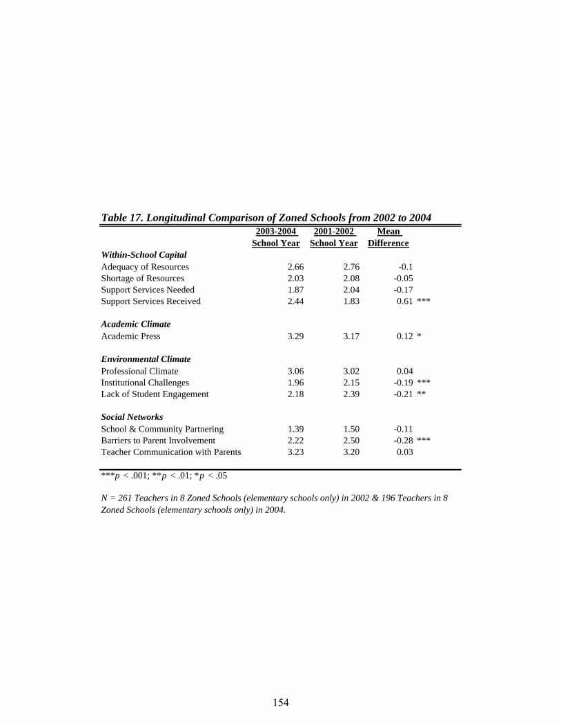
institutional challenges and more lack of student engagement when compared to other

zoned elementary schools. Enhanced option teachers rate institutional challenges as 2.13

on a scale of 1 to 4 (1 = Not at All and 4 = A Great Extent), whereas zoned elementary

school teachers rate institutional challenges as 2.12 (p < .01). Enhanced option teachers

also rate the lack of student engagement in the classes they teach as more problematic

than do zoned school teachers (enhanced option schools = 2.68 and zoned schools = 2.18

on a scale of 1-4 where 1 = Not at All and 4 = A Great Extent; p < .001). Concerning

social networks, teachers at enhanced option schools are more likely to engage in school

and community partnering (on a scale of 0-4 where 0 = Never and 4 = Almost Daily,

enhanced options = 1.62 and zoned schools = 1.45; p < .01). Barriers to parental

involvement and teacher communication with parents, however, were not significantly

different for enhanced option teachers and zoned elementary teachers.

When compared to zoned schools that have experienced the full range of changes

implemented as a result of unitary status, enhanced option schools seem to fare well in

terms of resources, but not as well in terms of academic and environmental climate.

Teachers in enhanced option schools are likely to report that the resources in their schools

are adequate and that they are more likely to partner with the community. However, as is

expected, enhanced option schools tend to be characterized by students who need many

social resources (not all of whom receive them), and they also tend to be less engaged in

school. Such conditions are likely to foster institutional challenges, as is reported by

enhanced option school teachers in this study.

149

Stability of Enhanced Option School Climate

Since enhanced option schools differ from zoned schools in typically negative

ways when considering their geographic and demographic characteristics, it is interesting

that they seem to differ in unusually positive ways in some of their school climate

characteristics. Thus, it is important to test the stability of the school climate in enhanced

option schools. The Metro school district was excited about implementing enhanced

option schools. When the first schools opened in the 1999-2000 school year, local

newspapers praised the efforts of these new school types (Long, 2002). The excitement

surrounding the schools was immense, and the district was dedicated to keeping their

commitments to these schools in terms of the additional resources provided. However,

the question remains: Is such a commitment to schools that are located in communities

that have so little sustainable over time? To assess sustainability, the Metro teacher

survey is used to compute independent sample t-tests21 on the responses of enhanced

option school teachers during the 2001-2002 school year versus responses in 2003-2004.

On average, teachers of enhanced option schools report significant different

results from 2002 to 2004 on three items: adequacy of resources, academic press, and

professional climate (see Table 16).22 Teachers report and increase in the adequacy of

resources available to them in their classrooms. On a scale of 1 to 4 where 1 =

Completely Inadequate and 4 = Completely Adequate, enhanced option teachers in 2002

reported a mean of 2.66, and a mean of 2.84 in 2004 (p < .05) (see Figure 11). It seems

21 In the Metro Teacher Survey, respondents are not linked over time; therefore, paired sample t-tests cannot be computed. 22 These trends are unique to enhanced option schools. The same analyses were conducted on a sample of zoned schools over time, and different results emerged. Teachers at zoned schools indicated that their resources were becoming less adequate over time, they received more support services, and that there were fewer barriers to parental involvement (see Table 17).

150

Table 16. Longitudinal Comparison of Enhanced Option Schools from 2002 to 2004

2003-2004 School Year

2001-2002 School Year

Mean Difference

Within-School CapitalAdequacy of Resources 2.84 2.66 0.18 *Shortage of Resources 2.05 2.07 -0.02Support Services Needed 3.04 2.91 0.13Support Services Received 2.32 2.53 -0.21

Academic ClimateAcademic Press 3.12 3.28 -0.16 *

Environmental ClimateProfessional Climate 3.00 3.13 -0.13 *Institutional Challenges 2.13 2.05 0.08Lack of Student Engagement 2.68 2.62 0.06

Social NetworksSchool & Community Partnering 1.62 1.64 -0.02Barriers to Parent Involvement 2.15 2.10 0.05Teacher Communication with Parents 3.12 3.07 0.05

***p < .001; **p < .01; *p < .05

N = 186 Teachers in 5 Enhanced Option Schools in 2002 & 167 Teachers in 5 Enhanced Option Schools in 2004.

151

Comparison of Trends in Enhanced Option Schools & Zoned Schools over Time

3.133.28

2.66

3.003.12

2.843.02

3.17

2.76

3.06

3.29

2.66

0

0.5

1

1.5

2

2.5

3

3.5

4

Adequacy ofResources*

Academic Press* ProfessionalClimate*

Adequacy ofResources

Academic Press* ProfessionalClimate

Scal

e

Enhanced Option 2002Enhanced Option 2004Zoned Schools 2002Zoned Schools 2004

Figure 11

152

that the school district continues to support and invest in enhanced option schools and

that these resources are noticed by teachers. Comparatively, zoned elementary schools

experienced a downward shift in the adequacy of their resources during this time period

(see Table 17 & Figure 11). However, teachers report significant downward shifts in

academic press and professional climate. One a scale of 1 to 4, teachers in 2002 reported

a mean of 3.28 on academic press and a mean of 3.12 in 2004 (p < .05). This difference

indicates a decline in the extent to which teachers feel responsible for students’ success

and for improving their school. Teachers also report a decrease in professional climate.

In 2002, enhanced option teachers reported a mean of 3.13 on a professional climate scale

(scale of 1-4). However, in 2004, teachers reported a mean of 3.00 (p < .05). This

decrease indicates that teachers collaborate less and are less likely to receive valuable

feedback and training to assist them with instructional practices. Interestingly, zoned

elementary schools experienced an increase in both academic press and professional

climate during the same time period. While enhanced option schools seem to be

receiving more adequate resources than zoned schools, the academic and professional

climate in these schools is declining over time, which is inconsistent with other

elementary schools in the district.

The only negative changes in enhanced option schools over time were the changes

related to teachers’ actions, attitudes, and morale. While the district has kept its financial

commitment to enhanced option schools, it seems that they have somewhat less control of

teachers’ experiences, motivation, and fatigue over time. It is worth noting that previous

analyses demonstrated that enhanced option schools experience the highest rates of

teacher turnover in the district. It may be that one of the most valuable educational

153

Table 17. Longitudinal Comparison of Zoned Schools from 2002 to 20042003-2004

School Year2001-2002

School YearMean

DifferenceWithin-School CapitalAdequacy of Resources 2.66 2.76 -0.1Shortage of Resources 2.03 2.08 -0.05Support Services Needed 1.87 2.04 -0.17Support Services Received 2.44 1.83 0.61 ***

Academic ClimateAcademic Press 3.29 3.17 0.12 *

Environmental ClimateProfessional Climate 3.06 3.02 0.04Institutional Challenges 1.96 2.15 -0.19 ***Lack of Student Engagement 2.18 2.39 -0.21 **

Social NetworksSchool & Community Partnering 1.39 1.50 -0.11Barriers to Parent Involvement 2.22 2.50 -0.28 ***Teacher Communication with Parents 3.23 3.20 0.03

***p < .001; **p < .01; *p < .05

N = 261 Teachers in 8 Zoned Schools (elementary schools only) in 2002 & 196 Teachers in 8 Zoned Schools (elementary schools only) in 2004.

154

resources—teachers—wear down over time. However, these negative differences from

2002 to 2004 place enhanced options schools about equally with zoned schools in 2004.

Continued monitoring of these changes in enhanced option schools is required to

determine the extent to which these downward trends continue in enhanced option

schools.

155

CHAPTER VII

CONCLUSIONS

This study offers a unique view of neighborhood contexts and their effects on

student outcomes. It offers an opportunity to explore educational, social, and political

relationships as one Southeastern school district shifts its priorities from cross-town

busing to unitary status. This shift in priorities was accompanied with dynamic changes

in the organization of education in Greensville. It is these dynamics that offer the context

for a study of the importance of the size of school attendance zones, the impact of the

social characteristics of a school’s attendance zone, and whether or not these social

characteristics can be mediated when students attend compensatory school. Findings

related to each of these issues are described in more detail below. Thereafter I outline

research-based implications of education policy as well as implications for social science

research.

Main Findings

This study focuses on three issues as they relate to student participation and

engagement in school: the importance of the size of school attendance zones, the impact

of the social characteristics of a school’s attendance zone, and whether or not these social

characteristics can be mediated when students attend compensatory schools.

156

When Schools are Closer to Home

As Greensville moved from court-ordered to court-ended desegregation, they

adopted a school improvement plan targeted at zoning children to schools that are closer

to their homes. Some researchers suggest that neighborhood schools, or schools that are

closer to students’ homes, offer a greater sense of place for students (for example, see

Driscoll, 2001; Morris, 2001). When a school is integrally a part of the larger

community, it can more easily address the needs of individual students living in specific

neighborhoods. Some also suggest that community schools offer avenues of increased

social capital as schools become the center for community life and interaction (Goldring

& Crowson, 2002; Driscoll, 2001). Therefore, schools that are closer to home should

foster a sense of place for children that can be observed through their participation and

engagement in school.

I find support for these hypotheses. School zones that are, on average, closer to

students homes are associated with an increase in student participation and engagement

which are observed through reduced absences and disciplinary events. When controlling

for the social and economic conditions of a school’s neighborhood, closer to home school

zones seem to foster a greater sense of place for students.

Neighborhoods Matter

The social disorganization literature addresses neighborhood conditions that

hinder the development of sense of place. Without a sense of place, neighborhoods

become areas characterized by crime, deviance, and lack of engagement in pro-social

behaviors. Undoubtedly, the characteristics of students’ school attendance zones

157

significantly impacted student participation and engagement. In fact, after controlling for

student and school characteristics, the social and economic context of schools’ attendance

zones accounted for much of the variation in students’ participation and engagement in

school. I find evidence for the social disorganization hypothesis in that students who

encountered schools characterized by economic deprivation were less likely to

participation and be engaged in school. Likewise students who encountered schools with

attendance zones characterized by residential stability, ethnic diversity, and social

advantage were more likely to be engaged and participate in school. Hence, the less

social disorganization inherent in a neighborhood, the more likely students are to

experience a sense of place through engagement and participation in schools.

This finding is meaningful in this particular study because a “neighborhood” is

defined as a school zone—a political boundary which is set to accomplish certain goals.

As such, these boundaries can be altered to reflect the social, educational, and political

goals of the larger community. Setting these boundaries in Greensville was an eight-year

community effort where collaboration and consensus building were the foci of attending

to the issues of educational and social priorities. When these boundaries are set, they

reflect the educational goals of a school district, and when these goals change, the

boundaries can be changed as well.

Unlike most definitions of “neighborhood” in the neighborhood effects literature,

identifying school zones provides an avenue through which neighborhood compositions

can be changed. When a school zone is changed, children’s patterns of interactions are

also changed, thereby broadening (or narrowing) their idea of “community.” Some

schools and school districts have resorted to the designation of school attendance zones

158

as a mechanism for enhancing educational equity (for example, Wake County, North

Carolina; Charleston, South Carolina; and Boston, Massachusetts), and preliminary

analyses suggest positive outcomes for students (though the effects of these

neighborhoods have not been measured directly as they are in this study) (Flinspach,

Banks, & Khanna, 2003; Willie, 1990).

The Role of Enhanced Option Schools

Returning to neighborhood schools for any school district that has been under a

court desegregation order involves significant shifts in the demographic composition of

schools. Inevitably, some schools will service populations of students living in

conditions of concentrated poverty. Underlying the idea of returning to high-poverty,

racially isolated, neighborhood schools is the notion that residents living in certain

neighborhood have specific needs in terms of educational and schooling and that those

needs can best be met within the context of their residential community. As Greensville

anticipated racially isolated, high-poverty schools when moving away from cross-town

busing, they looked to the possibility of full service schools to provide the necessary

resources to students who would begin school at an educational disadvantage based on

their family and community backgrounds. The idea here is that schools are able to “level

the playing field” when they provide disadvantaged children with the resources not

available in their homes and neighborhoods.

I find that enhanced option schools—in spite of their higher than average teacher

turnover rates, concentrations of poverty, and less desirable social conditions—have

positive effects on the children attending them. When students encounter an enhanced

159

option school, they are more likely to participate and be engaged in their schools. Even

though these schools are located in places one might describe as socially disorganized

(i.e., “bad neighborhoods”), they seem to have a positive influence in the lives of the

students attending them; however, this positive influence does not mediate the effects of

school neighborhoods in important ways. While enhanced option schools have been

found to mediate the effects of social advantage and residential stability, the degree to

which these effects are mediated is mild. In other words, enhanced option schools are

good schools with many resources (both academic and social); however, they are not

good enough to mediate the neighborhood characteristics of a school zone. It is

questionable that such schools would ever be able to mediate the devastating effects of

poverty and the associated social conditions.

While it appears that the district has been stalwart in keeping their promises of

additional physical and instructional resources in enhanced option schools, they seem to

have much less control over teacher turnover and morale in these schools. Thus, the one

thing that students do not receive when attending enhanced options schools is a stable

school environment. It is arguable that this would be one of the more important

“resources” a school could offer students—particularly when students attending these

schools tend to come from unstable home and neighborhood environments.

Implications for Education Policy

Currently, there is little evidence about whether a return to neighborhood schools

under unitary status provides benefits to students and whether those benefits are equally

distributed among all students. Additionally, there are virtually no empirical analyses of

160

unitary status plans—despite their growing popularity. National and regional data sets

have been used to track resegregation patterns after unitary status (see Orfield, 2001), yet

little is known about the consequences of specific policies associated with unitary status.

This study has attempted to do both—assess the benefits of neighborhood schools for all

students and simultaneously provide some evidence concerning the consequences of

widespread policies (i.e., the return to neighborhood schools) associated with unitary

status.

First, returning to neighborhood schools seems to be beneficial for establishing

social participation and engagement among students. However, the return to

neighborhood schools has serious consequences for children living in disadvantaged

school zones. While enhanced option schools alleviate some of these consequences, the

effects of racial isolation coupled with concentrated poverty are overwhelming. Metro

seems to represent the “best case scenario” in terms of the way unitary status was

achieved. Through collaboration and consensus building, the community and school

board worked together to derive a plan they thought they could all support. As such,

Greensville seems to be committed to the agreements reached when they were released

from their court order. As such, a grant of unitary status and a return to neighborhood

schools in any other school district may not be quite as successful. Even in Greensville,

the effects of unitary status are not yet clear. The next six to ten years will be equally

important in examining neighborhood effects as the six years included in this study, as

the excitement for the new SIP wanes and resources that are available now potentially

become less available in the future. It is still unclear how well enhanced option schools

161

will fare as the fatigue of working in such an environment affects the teachers and staff at

these schools.

When considering the adoption of enhanced option schools or any other types of

school-wide compensatory education strategies, policy makers must consider the

importance of social capital. While such schools in Greensville have received the

physical and instructional resources they need, they do not necessarily have the capacity

to support teachers and staff members in ways that are meaningful in their decision to

continue teaching in these schools. As such, stability and morale in these schools may be

lower than it could be. In other words, physical resources are not enough to maintain the

viability of compensatory schools.

This study also implies that the way policy makers draw school attendance zones

affects student outcomes because it defines the range of social interactions for children.

While many agree that closer-to-home schooling is an important educational priority, this

study also suggests the range of social interactions for students is also an important

priority. And, as is somewhat demonstrated in the case of Greensville, school zones can

be re-drawn in such ways that busing is limited (though not eliminated) and students

attend schools that are closer to their homes yet somewhat diverse in terms of

neighborhood composition. This however, does not mean necessarily that students would

attend schools that are closest to their homes.

Eventually, such issues must be addressed contextually. That is, all districts

facing similar problems must determine how they will address their educational priorities

and how they will establish equity in their schools. In general, I find positive outcomes

when children are sent to schools that are closer to their homes. I also find positive

162

outcomes for students attending enhanced options schools. However, neighborhood

contexts need to be better distributed when possible. The challenge for policy makers is

deciding on ways to address all three priorities: closer-to-home schooling, compensatory

services, and the distribution of social and economic neighborhood context (as they are

defined by school attendance zones). In reaching a balance among all three, it is

important to note that finding from this study suggest that compensatory services alone

do not mediate poor neighborhood conditions.

Implications for Social Science Research

This study also offers implications for social science research. Most importantly,

this study examines the interchange between neighborhoods and policies. While much of

the neighborhood effects research recommends changes in public policy as a result of

finding significant neighborhood effects for certain populations of people, few

researchers have examined the effects of these policies as mediator of neighborhood

effects (for example, see Crane, 1991a; Crane, 1991b). As is suggested by Sampson,

Morenoff, and Gannon-Rowley (2002), when studying neighborhood effects, indirect

relationships should also be explored. Mediating and moderating relationships may be

instrumental in determining how to best deal with the issues of concentrated poverty and

disruptive environments on the experiences and life chances of residents. Even though

this study detects mostly small mediated effects when considering the influence of

policies aimed at alleviating the effects of poor neighborhood conditions, it addresses the

issue of how difficult it might be to mediate these kinds of conditions without considering

zoning plans intended to foster the integration of neighborhood conditions. It would be

163

interesting to see if other organizational policies are able to mediate some of these

conditions in more significant ways.

Examining mediated relationships when determining the effects of neighborhood

characteristics on student outcomes also contributes to the sense of place and social

disorganization theories. As the theories are described in the literature, sense of place

and social disorganization occupy opposite ends of a “spectrum of community.”

However, this study has demonstrated that when resources and supports are made

available within the contexts of disadvantaged neighborhoods, evidence of “sense of

place” such as increased participation and engagement is likely to emerge. Therefore, it

is possible for geographic areas to be both socially disorganized—as is evidenced by

family disruption and economic deprivation, and well as the lack of residential stability

and social advantage—and for the people living in these areas to experience a sense of

place through their participation and engagement in public organizations. However,

these organizations—public schools, in this case—must be well maintained with

continued support. Otherwise, the duration through which these schools will be effective

mediators of social disorganization is unclear. Indeed, it may be that the only

“disorganized” communities are those with no infrastructure to facilitate participation and

engagement. Also, the best remedy for resident living in such communities may not be to

leave, as Park and Burgess (1925) have suggested. Rather, the best remedy may include

social and economic investments in the public organizations available in such areas. In

other words, a socially disorganized neighborhood may be an ignored neighborhood.

And it is possible for residents of such a disorganized neighborhood to exhibit

characteristics associated with sense of place. “All places, no matter what else they have,

164

have a sense of shared experience” (Lewis, 1979, p. 41), and, for children, those shared

experiences begin with their participation and engagement in school. What researchers

would identify as a “socially disorganized” neighborhood is an area that residents of

those neighborhoods call “home” (see Furstenberg, et al., 1999). As such, one cannot

instinctively assume that sense of place—evidenced in residents’ participation and social

engagement—is absent in the presence of social disorganization.

In a time where “place” often has political boundaries—that is, people’s patterns

of interactions are often influenced by boundaries that are politically defined rather than

geographically defined (though the two types of boundaries tend to be related to one

another), it is important that researchers seek to define “neighborhoods” more

contextually. Using school attendance zones as neighborhood boundaries is an example

of one way to define people’s range of social interactions (Sampson, Morenoff, &

Gannon-Rowley, 2002). However, these boundaries are infinitely more difficult to

identify and measure than are the typical “boundaries” used in neighborhood research (5-

digit zip codes, for example). Nevertheless, using such boundaries in research offers

implications for how these boundaries can be structured.

According to Wilson (1998), the challenge for social scientists is to develop new

frameworks that consider the complex interrelationships between individual behaviors

and social-structural characteristics. This study specifically identifies individual

behaviors as a function of the social-structural characteristics of educational priorities and

policies as well as neighborhoods as defined by school attendance zones. As such, it is

clear that children’s environments affect school-related outcomes at very early ages. It is

the responsibility of researchers and policy makers to consider more seriously the

165

consequences of how children’s “places”, and consequently their ranges of social

interactions, are defined. Both closeness to home and diversity in school zones are noble

goals; however, both extremes have been demonstrated to have negative consequences

for children. To facilitate greater participation and engagement in schools as well as in

the larger society, distance from home, social and economic diversity, and compensatory

services must all be considered together as mechanisms for fostering stable and

meaningful places for children.

166

Appendix A. Sample of Students by Year, Grade, and School Type

Year GradeNeighborhood

SchoolsMagnet Schools

Enhanced Option Schools

Design Centers Total

1999K 5682 210 0 0 58921 6163 142 0 0 63052 5871 119 0 0 59903 5985 104 0 0 60894 5654 95 0 0 57495 4364 788 0 0 51526 4153 743 0 0 48967 4793 540 0 0 53338 4362 488 0 0 48509 4818 864 0 0 568210 3327 639 0 0 396611 2798 545 0 0 334312 2490 501 0 0 2991

Total 60460 5778 0 0 66238% 91% 9% 0% 0% 100%

2000K 5308 365 212 71 59561 5731 240 215 66 62522 5361 170 313 38 58823 5722 156 119 37 60344 5652 139 111 45 59475 4352 1034 94 48 55286 4080 948 92 39 51597 4636 655 0 0 52918 4432 491 0 0 49239 4720 972 0 0 569210 3428 721 0 0 414911 2737 550 0 0 328712 2590 518 0 0 3108

Total 58749 6959 1156 344 67208% 87% 10% 2% 1% 100%

167

Appendix A (continued). Sample of Students by Year, Grade, and School Type

Year GradeNeighborhood

SchoolsMagnet Schools

Enhanced Option Schools

Design Centers Total

2001K 5101 282 261 297 59411 5192 192 266 259 59092 5194 220 221 284 59193 5099 154 212 245 57104 5153 162 202 227 57445 4780 748 17 33 55786 4475 731 6 33 52457 4476 624 0 0 51008 4243 597 0 0 48409 4663 996 0 0 565910 3249 753 0 0 400211 2785 612 0 0 339712 2514 531 0 0 3045

Total 56924 6602 1185 1378 66089% 86% 10% 2% 2% 100%

2002K 4983 237 354 273 58471 5056 219 376 338 59892 4783 198 331 290 56023 4983 220 317 287 58074 4931 149 310 250 56405 4850 699 36 0 55856 4665 751 47 0 54637 4683 656 0 0 53398 4264 581 0 0 48459 4754 932 0 0 568610 3342 743 0 0 408511 2730 638 0 0 336812 2573 605 0 0 3178

Total 56597 6628 1771 1438 66434% 85% 10% 3% 2% 100%

168

Appendix A (continued). Sample of Students by Year, Grade, and School Type

Year GradeNeighborhood

SchoolsMagnet Schools

Enhanced Option Schools

Design Centers Total

2003K 4852 292 387 344 58751 4881 175 346 321 57232 4807 211 362 366 57463 4608 189 323 321 54414 4824 210 314 311 56595 4443 763 0 89 52956 4605 742 0 88 54357 4446 806 0 52 53048 4383 711 0 1 50959 4845 1021 0 0 586610 3441 806 0 0 424711 2885 672 0 0 355712 2634 662 0 0 3296

Total 55654 7260 1732 1893 66539% 84% 11% 3% 3% 100%

2004K 5004 189 522 420 61351 4667 185 477 412 57412 4609 180 429 373 55913 4660 201 423 407 56914 4499 181 363 361 54045 4288 712 0 399 53996 4179 675 0 346 52007 4254 743 0 361 53588 4267 762 0 83 51129 5082 978 0 0 606010 3514 820 0 0 433411 2994 725 0 0 371912 2752 671 0 0 3423

Total 54769 7022 2214 3162 67167% 82% 10% 3% 5% 100%

169

Appendix A (continued). Sample of Students by Year, Grade, and School Type

Year GradeNeighborhood

SchoolsMagnet Schools

Enhanced Option Schools

Design Centers Total

All YearsK 30930 1575 1736 1405 356461 31690 1153 1680 1396 359192 30625 1098 1656 1351 347303 31057 1024 1394 1297 347724 30713 936 1300 1194 341435 27077 4744 147 569 325376 26157 4590 145 506 313987 27288 4024 0 413 317258 25951 3630 0 84 296659 28882 5763 0 0 3464510 20301 4482 0 0 2478311 16929 3742 0 0 2067112 15553 3488 0 0 19041

Total 343153 40249 8058 8215 399675% 86% 10% 2% 2% 100%

All Years, Grades 3-83 31057 1024 1394 1297 347724 30713 936 1300 1194 341435 27077 4744 147 569 325376 26157 4590 145 506 313987 27288 4024 0 413 317258 25951 3630 0 84 29665

Total 168243 18948 2986 4063 194240% 87% 10% 2% 2% 100%

% of District Total 42% 5% 1% 1% 49%

Working Sample: All Years, Grades 3-8, Neighborhood & Enhanced Option Schools Only3 31057 0 1394 0 324514 30713 0 1300 0 320135 27077 0 147 0 272246 26157 0 145 0 263027 27288 0 0 0 272888 25951 0 0 0 25951

Total 168243 0 2986 0 171229% 98% 0% 2% 0% 100%

% of District Total 42% 0% 1% 0% 43%

170

Appendix B. Teacher Survey

171

REDEFINING COMMUNITIES: THE RE-ZONING OF METROPOLITAN NASHVILLE PUBLIC

SCHOOLS

A SURVEY OF METRO NASHVILLE TEACHERS

2001-2002 School Year Survey

Conducted by the Department of Leadership & Organizations Peabody College of Education, Vanderbilt University

172

CLASSROOM RESOURCES We are interested in the instructional resources that are currently available to you as a classroom teacher during this academic year. Please check the box that best represents your answer.

Q.1 Do you have textbooks for every student in your classroom?

1-Yes 2-No 3- Not Applicable

Q.2 Do you have workbooks for every student in your classroom?

1-Yes 2-No 3-Not Applicable

Q.3 Other than text and reference books, does the school provide subject-specific curricular materials for your classroom (e.g. maps, lab equipment, calculators, scientific equipment, musical instruments, etc)

1-Yes – Please specify __<--_Q.3spec___________________________________________________

2-No

3- Not applicable

Q.4 How many functioning computers does your school provide for your classroom that are

capable of running all the programs that you would like to use? _____

Q.5 Is there a computer room in your school?

1-Yes Q.5a If there is a computer room, do you have access to it for instructional purposes?

2-No 1-Yes 2-No

Q.6 Is there a curriculum/Instruction specialist (e.g. reading specialist, math support teacher, etc) at your school?

Q.6a If your school has a curriculum specialist, do you utilize this person to help you with lesson planning, lesson development and other related activities?

1-Yes

2-No

1-Yes 2-No

Q.7 Is there a teacher workroom or area at your school?

1-Yes Q7a. If your school has a teacher workroom or area, do you utilize it for your class preparations?

2-No 1-Yes 2-No

173

Q.8 How adequately does your school provide you with each of the following resources for your classroom?

Not Applicable

Completely Inadequate

Mostly Mostly Completely Adequate

(Circle one number for each item) Inadequate Adequate

Q.8a Basic supplies (paper, chalk, markers)

1 2 3 4 5

Q.8b Current, adopted materials (texts)

1 2 3 4 5

Q.8c Supplemental texts (e.g. 1 2 3 4 5

workbooks) Q.8d Reference materials in my classroom (Maps, science kits, math manipulatives)

1 2 3 4 5

Q.8e Subject-specific supplemental1 2 3 4 5

materials Q.8f TV/VCR Accessibility in my classroom

1 2 3 4 5

Q.8g Computers in my classroom 1 2 3 4 5

Q.8h Computer printer in my classroom

1 2 3 4 5

Q.8i Educational software in my classroom

1 2 3 4 5

Q.8j An Internet connection in my classroom

1 2 3 4 5

Q.8k Technical (computer) support 1 2 3 4 5

Q.8l Teacher educational assistant 1 2 3 4 5

Q.8m Calculators 1 2 3 4 5

Q.9 Are you working with any non-district programs in your classroom (e.g. School &

university partnerships, test preparation programs, privately developed instructional or curricular materials, etc.)?

1-Yes Please Specify:

2-No Programs: <-- _Q.9prog_________________________________

Curriculum and or Instructional Materials: <--_Q.9curr________________________

Partnerships: <--_Q.9part________________________________

Other: <-- Q.9othe______________________________________

Q.10 What other resources, crucial to your instructional capacity, are you presently USING?

_________________________________________________________________________________

Q.11 What resources, crucial to your instructional capacity, are you presently LACKING?

_________________________________________________________________________

174

Q.12 How often do your children use the following materials or resources in your typical class?

(Circle one number for each item) Not

available Never Once a month or less

Two or three

times a month

Once or twice a week

Three or four

times a week

Daily

Q.12a Textbooks 1 2 3 4 5 6 7

Q.12b Tradebooks 1 2 3 4 5 6 7

Q.12c Workbooks and practice sheets

1 2 3 4 5 6 7

Q.12d Manipulatives (e.g., blocks, puzzles)

1 2 3 4 5 6 7

Q.12e Audiovisual equipment (e.g., VCR, audio tapes)

1 2 3 4 5 6 7

Q.12f Computer equipment 1 2 3 4 5 6 7

Q.12g Musical recordings 1 2 3 4 5 6 7

Q.12h Paper and pencils 1 2 3 4 5 6 7

Q.12i Art materials (e.g. paints, clays, etc)

1 2 3 4 5 6 7

Q.12j Musical instruments 1 2 3 4 5 6 7

Q.12k Television 1 2 3 4 5 6 7

Q.12l Calculators 1 2 3 4 5 6 7

Q.13 About what percentage of your students need the following types of support services in your most typical class?

(Circle one number foreach item)

Less than 25% 25% to 45% About 50%

55% to 75% More than 75%

Q.13a Academic Tutoring

1 2 3 4 5

Q.13b Mentoring 1 2 3 4 5

Q.13c Health Services

1 2 3 4 5

Q.13d Social Services

1 2 3 4 5

Q.13e Testing for SPED

1 2 3 4 5

Q.13f Other (specify) Q.13oth__

1 2 3 4 5

175

Q.14 About what percentage of the students in your most typical class who need the following support services actually receive them?

(Circle one number foreach item)

About 50%

Less than 25% 25% to 45% 55% to 75% More than 75%

Academic Q.14a 1 2 3 4 5

Tutoring

Q.14b Mentoring 1 2 3 4 5

Health Q.14c 1 2 3 4 5

Services

Social Services

Q.14d 1 2 3 4 5

Testing for Q.14e 1 2 3 4 5

Special ed.

Other (specify)

Q.14f 1 2 3 4 5 ____________

INSTRUCTION

In this section we are interested in instructional issues in your classroom. Please check the box that best represents your answer.

in a typical weekQ.15 Indicate about what percent of your time is spent doing each of the following with your most typical class. (Reponses may not add up to exactly 100%)

None <10% 10-24% 25-49% 50-74% 75-100%

Q.15a Providing instruction to the class

1 2 3 4 5 6 as a whole

Providing instruction to small groups of students Q.15b 1 2 3 4 5 6

Q.15c Providing instruction to individua

1 2 3 4 5 6 students

Maintaining order or discipliningstudents Q.15d 1 2 3 4 5 6

Q.15e Administering tests or quizzes 1 2 3 4 5 6

Performing routine administrativtasks (e.g. taking attendance, making announcements, etc.)

Q.15f 1 2 3 4 5 6

Q.15g Conducting lab periods 1 2 3 4 5 6

Q.15h Other non-instructional activitie 1 2 3 4 5 6

Q.15i Standardized test preparation 1 2 3 4 5 6

176

Q.16 To what extent do you use each of the following strategies when working with students of different achievement levels?

Small extent

Moderate extent

Great Extent

(Circle one number for each item) Not at all

Q.16a Homogenous grouping 1 2 3 4

Q.16b Extra time with low-performers 1 2 3 4

Q.16c Different instruction materials 1 2 3 4

Q.16d One-on-one instruction 1 2 3 4

Q.16e Frequent assessments of performance 1 2 3 4

Higher achieving students work with lower achieving students

Q.16f 1 2 3 4

PROFESSIONAL CLIMATE

We are interested in the climate among faculty at your school during this academic year. Please check the box that best represents your answer.

Q.17 How many professional leave days did you use last school year? _____

Q.18 How many CODE 10 days did you participate in last school year? _____

Q.19 How many summer workshops did you attend in 2001? _____

2001Q.20 How many hours did you spend in summer workshops in ? _____

Q.21 This school year (2001 – 2002), how often do you have scheduled meetings with other teachers in this school to discuss and plan curriculum or teaching approaches?

1- Never

2- Once or twice a year

3- Once every other month

4- Once a month

5- 2 – 3 times a month

6- Once a week

7- More than once a week

177

Q.22 Please mark the extent to which you agree or disagree with each of the following statements about the teachers in your school.

(Circle one number for each item) Strongly disagree

Disagree Agree Strongly Agree

Q.22a Most teachers are continually learning and seeking new ideas.

1 2 3 4

Q.22b Most teachers make a conscious effort to coordinate their teaching with instruction at other grade levels.

1 2 3 4

Q.22c Most teachers are supported in their efforts to experiment and develop new programs and curricula.

1 2 3 4

Q.22d When teachers are not doing a good job, the principal works with them to improve instruction. 1 2 3 4

Q.22e Performance evaluation procedures in this school help teachers grow professionally. 1 2 3 4

Q.22f My principal is available when I need to see him/her. 1 2 3 4

Q.22g Other teachers encourage me to try out new ideas. 1 2 3 4

Q.22h Teachers receive the help they need from the principal when problems arise. 1 2 3 4

Q.22i The principal spends time in my classroom observing my teaching and provides feedback. 1 2 3 4

Q.22j In-service training and staff development programs in this school help teachers grow professionally. 1 2 3 4

Q.22k The staff is continually evaluating its programs and activities. 1 2 3 4

Q.23 On average, how many hours per week, do you have for collaborative planning?

________ hours.

Q.23a Percentage of your total planning time, in a typical week, is consumed by other school

activities (e.g., tutoring, meetings, etc)? ________%

178

RACIAL CLIMATE IN SCHOOL

In this section we are interested in learning more about the racial climate in your classroom or school, during the present school year. Q.24 Please mark the appropriate box that best describes the percentage of minority

students in your most typical class. (Minority refers to African American, Hispanic, Asian, Pacific Islander, Native American and/or Alaskan Native.)

1-Less than 20% minority

2-Between 21 and 40% minority

3-Between 41 and 60% minority

4-Between 61 and 80% minority

5-Between 81 and 90% minority 6-Between 91% and greater Skip to question Q26. Q.25 Please indicate the extent to which each of the following statements applies to your

most typical CLASS. (Minority refers to African American, Hispanic, Asian, Pacific Islander, Native American, or Alaskan native students.)

(Circle one number for each item) Never Rarely Always Sometimes

Minority and white students work together on group 1 2 3 4 Q.25a

assignments.

Interracial conflicts are a problem in my class. 1 2 3 4 Q.25b

Minority and white students participate equally in class 1 2 3 4 Q.25c

discussions.

Students make friends with students of other racial and/or ethnic groups in my class. 1 2 3 4 Q.25d

Minority students (who are not receiving ELL services) and 1 2 3 4 Q.25e

white students achieve at about the same level.

I often overhear students making racist remarks. 1 2 3 4 Q.25f

179

Q.26 For this next question, we would like you to consider your school as a whole. Please indicate the extent to which each of the following statements applies to YOUR SCHOOL. (Minority refers to African American, Hispanic, Asian, Pacific Islander, Native American, or Alaskan native students.)

(Circle one number for each item) Never Rarely Sometimes Always

Q.26a Minority students sit and/or converse with white students at lunchtime. 1 2 3 4

Q.26b Interracial conflicts are a problem at this school. 1 2 3 4

Q.26c Minority and white students play together at recess or free time. 1 2 3 4

Q.26d Minority and white students achieve at about the same level. 1 2 3 4

Q.26e Students make friends with students of other racial and ethnic groups. 1 2 3 4

Q.26f Fights often occur between different racial or ethnic groups. 1 2 3 4

Q.26g Students of different races form after school friendships. 1 2 3 4

Q.26h Students of different races can be found in the same clubs and activities. 1 2 3 4

Q.26i Racial and/or ethnic differences among staff members create tensions at this school. 1 2 3 4

Q.26j I often overhear students making racist remarks. 1 2 3 4

180

ENVIRONMENTAL CLIMATE

In this next section we would like to ask you a series of questions regarding the present climate of your school during this school year.

Q.27 Which of the following limit you in how you teach your most typical class?

Small extent

Moderate extent

Great Extent

(Circle one number for each item) Not at all

Q.27a Low morale among fellow teachers/administrators 1 2 3 4

Students who come from a wide range of backgrounds Q.27b 1 2 3 4

Q.27c Threat(s) to personal safety or safety of students 1 2 3 4

Q.27d The noise level in the school building 1 2 3 4

Amount of professional support staff (e.g., Q.27e 1 2 3 4

counselors, specialists)

Students with special needs (e.g., hearing, vision, speech impairment, physical disabilities, mental or emotional/psychological impairment)

Q.27f 1 2 3 4

Q.27g Amount of time to prepare for class 1 2 3 4

Q.27h High student/teacher ratio 1 2 3 4

Q.27i Students with different academic abilities 1 2 3 4

Q.27j Uninterested students 1 2 3 4

Q.27k Disruptive students 1 2 3 4

Parents uninterested in their children’s learning progress Q.27l 1 2 3 4

Q.27m Shortage of computer hardware 1 2 3 4

Q.27n Shortage of computer software 1 2 3 4

Shortage of other instruction equipment for students’ Q.27o 1 2 3 4

use

Shortage of equipment for your use in demonstrations and other exercises Q.27p 1 2 3 4

Q.27q Inadequate physical facilities 1 2 3 4

Q.27r Low morale among students 1 2 3 4

181

SCHOOL AND CLASSROOM INFORMATION

In this section, we will ask you for some general school and classroom information.

Q.28 Which of the following best describes THIS school? (Check one)

1-Magnet school

2-Magnet within school program

3-Enhanced option school

4-Laboratory school

5-Design center school

6-Regular neighborhood/zone school

7-Title I neighborhood/zone school

Q.29 Which of the following best describes your MAIN assignment at this school during this school year? (Check one)

1-Full-time teacher 2-Part-time teacher or Job Share 3-Itinerant teacher (provide instruction at more than one school site) 4-Educational Assistant 5-Substitute 6-Administrator 7-Librarian/Media Specialist 8-Support Staff

9-Other professional staff, please specify _<--Q.29oth____________________________________

Q.30 Which of the following best describes most of your classes at YOUR CURRENT SCHOOL?

1-Self-contained Class – you teach multiple subjects to the same students

2-Team Teaching – you collaborate with one or more teachers in teaching multiple subjects to the same students

3-Pull Out Class – you teach certain students who are released from their regular classes (gifted, remedial, special education)

4-Departmentalized Classes – You teach one or more subject matter courses to several classes of different students all or most of the day

What Subject? <-- Q.30sub_______

182

Q.31 What is the total number of class periods that you are the primary instructor during

a typical day? __________

Q.32 What type of certificate do you hold in you MAIN assignment field?

1-Regular of standard state certificate or advanced professional certificate

2-Probationary certificate [the initial certificate issued after satisfying all requirements except the completion of the probationary period

3-Provisional or other type given to persons who are still participating in what the state calls an “alternative certification program.”

4-Temporary certificate (requires some additional college coursework and/or student teaching before regular certification can be obtained.

5-Emergency certificate or waiver (issued to persons with insufficient teacher preparation who must complete a regular certification program in order to continue teaching).

Q.33 Do you teach outside this main teaching assignment field?

1-Yes

2-No

Q.33a How many class periods? _______

Q.33b What subject? ____________________

ACADEMIC PRESS

In this next section we would like to ask you a series of questions regarding the extent to which your school emphasizes academic achievement.

Q.34 How many teachers at this school:

Almost none

Nearly All

(Circle one number for each item) Some Most

Q.34a Feel responsible when students fail? 1 2 3 4

Q.34b Feel responsible to help each other do their best? 1 2 3 4

Help maintain discipline in the entire school, not just their classroom? Q.34c 1 2 3 4

Q.34d Take responsibility for improving the school? 1 2 3 4

Feel responsible for helping students develop self-control? Q.34e 1 2 3 4

Q.34f Set high standards for their own performance? 1 2 3 4

Q.34g Feel responsible that all students learn? 1 2 3 4

183

PARENT INVOLVEMENT

In this next section we would like to ask you a series of questions regarding the involvement of parents in your school.

how manyQ.35 Please indicate of your students’ parents do you contact in the following ways in a typical week:

Q.35a Phone call, written note, or e-mail exchanges with parents (excluding required forms)

____

Q.35b Face-to-face meetings with parents (excluding regularly scheduled parent-teacher

conferences ________

Q.35c Since September how many visits, if any, have you made to a student’s home?

________

Q.36 How often do you interact with parents from this school in the following ways?

(Circle one number for each item) Never Rarely Sometimes Often

Q.36a In church or at church activities 1 2 3 4

Through community sports programs or other non-school related activities.

Q.36b 1 2 3 4

Q.36c By living in the same neighborhood. 1 2 3 4

Through contacts or chance meetings such as the supermarket.

Q.36d 1 2 3 4

Q.36e Other (please specify) ___________________________ 1 2 3 4

Q.37 During this school year, how easy has it generally been to contact parents when you wanted to talk with them about their child?

1-Very easy 2-Easy 3-A little difficult 4-Difficult 5-Very difficult

184

Q.38 How often do each of the following affect parent involvement at this school?

(Circle one number for each item) Never Rarely Sometimes Often

Q.38a The distance parents have to travel from their home to theschool is too far. 1 2 3 4

Q.38b Parents do not feel welcome at this school. 1 2 3 4

Q.38c Parents’ work schedules conflict with meeting and conference times at the school. 1 2 3 4

Q.38d Parent apathy. 1 2 3 4

Q.38e Lack of transportation for children 1 2 3 4

Q.38f Lack of childcare 1 2 3 4

Q.38g Other (please specify) ____________________________ 1 2 3 4

Q.39 How would you rate your school’s neighborhood in terms of safety for your students?

1-Very Safe 2-Somewhat Safe 3-Somewhat Unsafe 4-Very Unsafe

Q.40 How would you rate your school’s neighborhood in terms of safety for yourself?

1-Very Safe 2-Somewhat Safe 3-Somewhat Unsafe 4-Very Unsafe

Q.41 Teachers may communicate many different types of information to their students’ families. How often do you communicate the following information to parents of your students?

(Circle one number for each item) Never Sometimes Usually Always

Q.41a Inform parents about learning objectives in core academic subjects

1 2 3 4

Q.41b Contact parents when their child is encountering academic problems

1 2 3 4

Q.41c Provide parents with examples of excellent student work 1 2 3 4

Q.41d Provide parents with specific activities for children and parents to do to improve students’ grades

1 2 3 4

Q.41e Assign homework that requires children to interact with parents

1 2 3 4

Q.41f Other (please specify) Q.41oth_______________ 1 2 3 4

185

Q42. This school year, how often have you:

A few times a

year

Once or twice a month

Once of twice a week

Almost daily

Never (Circle one number for each item)

Brought in a guest speaker from the school’s Q.42a 1 2 3 4 5

community

Talked with students about people and/or events in the community

Q.42b 1 2 3 4 5

Q.42c Consulted with members of the community to

1 2 3 4 5 better understand your students

Taken students on a field trip to a local site or organization Q.42d 1 2 3 4 5

Q.42e Talked with students about their cultures 1 2 3 4 5

Q.42f Talked with students about their lives at home 1 2 3 4 5

Q.42g Talked with students about issues and concern

1 2 3 4 5 in the school’s community

STUDENT CHARACTERISTICS

Q.43 Are all of the students in your MAIN ASSIGNMENT field classes in the same grade?

1-Yes 2-No

Q.43a How many total students do you teach in a typical day? ________.

Q.44 What are the grade levels of the majority of the students in your MAIN ASSIGNMENT field class(es)? Circle all that apply.

Grade: Pre K K 1 2 3 4 5 6 7 8

(1-if circled, 0-if not)

Q.45 Think about a typical class that you teach.

Q.45a How many students are enrolled? ______

Q.45b How many students receive services for exceptionalities other than gifted education or

E.L.L.? ______

Q.45c How many students qualify for free and reduced price lunch? _________

186

Q.45d How many students receive services for gifted exceptionalities? __________

Q.45e How many students can be identified as English Language Learners? _________

Q.45f Of those receiving English Language Learner services, how many languages, other than

English are spoken in you most typical class? _________

PERSONAL INFORMATION

In this section, we are interested in some background information about you.

Q.46 How many years have you served as a full-time public school teacher, including this year?

__________

Q.47 Are you a Title I teacher? 1-Yes 2-No

Q.48 How many years have you served as a full-time public school teacher in Metro Nashville schools, including this year?

__________

Q.49 How many years have you taught at this school, including this year, but excluding student teaching?

__________

Q.50 What is your base salary this year?

5- $55,001 and above

4-Between $45,001 and $55,000

3-Between $35,001 and $45,000

2-Between $30,001 and $35,000

1-Between $25,000 and

$30,000

Q.51 What statement best describes how you got a position at this school?

1- I chose this school over positions at other schools because I wanted to teach here.

2- This was the only school with an opening I qualified for.

3- I was assigned to this school.

4- Other: Please specify ________________________________________________

Q.52 What is the highest degree that you have earned?

1-Bachelors 2-Masters 3-Masters +30 hours 4-Professional Diploma 5-Doctorate

187

Q.53 Are you presently pursuing coursework related to the field of education?

1-Yes 2-No

Q.54 Please indicate the three most important reasons why you are teaching at this school, by ranking your selections from 1 to 3 (1 being the most important reason you chose to work at your present school).

Q.54.1 _____ I was assigned to this school.

Q.54.2 _____ I was attracted by the reputation of the students.

Q.54.3 _____ I was attracted by the reputation of the schools administration.

Q.54.4 _____ I was attracted by the school’s instructional program.

Q.54.5 _____ I wanted to teach with this school’s staff.

Q.54.6_____ The school is in a good neighborhood.

Q.54.7 _____ I was unhappy with my former school.

Q.54.8 _____ This school was closer to my home.

Q.54.9 _____ I was attracted by the challenge of teaching at this school.

Q.54.10 _____ Other (please specify) _________________________________________

Q.55 What racial or ethnic group do you identify with? ________________________

Q.56 What is your gender? 1-male 2-female

In the space provide below, please feel free to provide any comments

188

ScID

VU

ID

Date

189

Appendix C. HLM & HCM Model Notation & Equations HCM Growth Models (full models) Level 1 Portion of Model (time varying student model):

E(Student Absences B) = 8 Log[8] = Y (1.1) Ytij(Student Absences) = B0ij + B1ij(Time)ti + B2ij(Grade)ti + B3ij(IEP)ti + B4ij(LEP)ti + etij, etij ~ N(0, F2)

Row & Column Portion of Model (time invariant model): B0ij = 20 + b00i + c00j + ((01ij) Free & Reduced Lunch + ((02ij) African American + ((03ij) Other Races

+ ((04ij) Female + (β01j) 75% Black + (β02j) School Size + (β03j) Teacher Turnover (1.2) + (β04j) School Zone Distance + (β05j) Residential Stability + (β06j) Ethnic Diversity + (β0ij) Social Advantage + (β08j) Economic Deprivation + (β09j) Enhanced Option School

B1ij = 21

B2ij = 22

B3ij = 23

B4ij = 24 HLM Growth Model Level 1 Portion of Model:

Yij(School Zone Distance) = B0j + B1j(Time) + e (2.1) Level 2 Portion of Model:

B0j = $00 + r0 (2.2)

B1j = $10 + r1

190

Appendix D1. Description of School Zone Contexts over Time

School YearStability

Mean

Ethnic Diversity

Mean

Family Disruption

Mean

Social Advantage

Mean

Economic Deprivation

Mean

Distance Between Home

& School

Number of BGs in School

Zone

Enhanced Option School

1 1999 0.29 0.34 0.36 0.31 0.34 3.43 26 02000 0.29 0.34 0.36 0.31 0.34 3.43 26 02001 0.36 0.31 0.35 0.31 0.29 3.86 33 02002 0.43 0.27 0.39 0.30 0.28 3.43 26 0

Change* 0.15 -0.07 0.04 -0.01 -0.06 0.00 0

2 1999 0.43 0.38 0.46 0.21 0.29 3.73 20 02000 0.43 0.38 0.46 0.21 0.29 3.73 20 02001 0.43 0.36 0.46 0.21 0.29 3.84 22 02002 0.41 0.37 0.46 0.18 0.29 2.40 11 02003 0.41 0.37 0.46 0.18 0.29 2.40 11 02004 0.41 0.37 0.46 0.18 0.29 2.40 11 0

Change* -0.02 0.00 0.00 -0.03 -0.01 -1.33 -9

3 2000 0.41 0.41 0.28 0.30 0.18 6.63 24 02001 0.40 0.41 0.29 0.30 0.18 6.72 24 02002 0.41 0.41 0.29 0.29 0.18 6.41 23 02003 0.42 0.40 0.30 0.30 0.18 6.41 24 02004 0.42 0.40 0.30 0.30 0.18 6.41 23 0

Change* 0.01 -0.01 0.02 0.00 0.00 -0.22 -1

4 2002 0.42 0.40 0.45 0.23 0.34 2.58 27 02003 0.42 0.39 0.43 0.25 0.33 2.58 24 02004 0.42 0.39 0.43 0.25 0.33 2.58 24 0

Change* 0.01 -0.01 -0.02 0.02 -0.02 0.00 -3

5 1999 0.43 0.34 0.44 0.20 0.29 6.38 37 02000 0.43 0.34 0.44 0.20 0.29 6.38 37 02001 0.48 0.35 0.50 0.18 0.31 5.40 36 02002 0.51 0.37 0.56 0.13 0.32 2.40 15 02003 0.51 0.37 0.56 0.13 0.32 2.40 15 02004 0.51 0.35 0.58 0.12 0.35 2.68 18 0

Change* 0.07 0.01 0.14 -0.08 0.06 -3.69 -19

6 1999 0.36 0.40 0.34 0.30 0.24 7.29 21 02000 0.43 0.37 0.33 0.28 0.25 5.93 18 02001 0.43 0.45 0.25 0.35 0.15 4.85 12 02002 0.45 0.44 0.23 0.35 0.15 4.46 11 02003 0.45 0.44 0.23 0.35 0.15 4.46 11 02004 0.45 0.44 0.23 0.35 0.15 4.46 11 0

Change* 0.09 0.03 -0.10 0.05 -0.09 -2.82 -10

191

Appendix D1 (continued). Description of School Zone Contexts over Time

School YearStability

Mean

Ethnic Diversity

Mean

Family Disruption

Mean

Social Advantage

Mean

Economic Deprivation

Mean

Distance Between Home

& School

Number of BGs in School

Zone

Enhanced Option School

7 1999 0.48 0.20 0.29 0.42 0.24 10.56 46 02000 0.48 0.20 0.29 0.42 0.24 10.56 46 02001 0.44 0.21 0.35 0.41 0.24 8.56 24 02002 0.44 0.21 0.35 0.41 0.24 8.56 24 02003 0.45 0.19 0.43 0.38 0.27 8.60 28 02004 0.45 0.18 0.40 0.41 0.25 8.64 26 0

Change* -0.03 -0.02 0.10 -0.01 0.01 -1.92 -20

8 1999 0.52 0.34 0.51 0.26 0.31 4.68 9 02000 0.52 0.34 0.51 0.26 0.31 4.68 9 02001 0.53 0.40 0.39 0.31 0.25 4.66 7 02002 0.52 0.38 0.38 0.31 0.24 4.85 8 02003 0.52 0.38 0.38 0.31 0.24 4.85 8 02004 0.52 0.38 0.38 0.31 0.24 4.85 8 0

Change* 0.00 0.04 -0.13 0.05 -0.07 0.17 -1

9 1999 0.49 0.30 0.36 0.32 0.26 2.63 16 02000 0.49 0.30 0.36 0.32 0.26 2.63 16 02001 0.49 0.30 0.36 0.32 0.26 2.63 16 02002 0.50 0.30 0.39 0.31 0.27 2.72 17 02003 0.49 0.31 0.41 0.31 0.27 2.95 21 02004 0.50 0.31 0.39 0.32 0.25 2.90 20 0

Change* 0.01 0.01 0.03 0.00 0.00 0.26 4

10 1999 0.60 0.30 0.56 0.21 0.34 2.62 10 02000 0.60 0.30 0.56 0.21 0.34 2.62 10 02001 0.60 0.30 0.56 0.21 0.34 2.62 10 02002 0.59 0.35 0.55 0.20 0.35 2.19 7 12003 0.59 0.35 0.55 0.20 0.35 2.19 7 12004 0.59 0.35 0.55 0.20 0.35 2.19 7 1

Change* -0.01 0.04 -0.01 -0.01 0.01 -0.43 -3

11 1999 0.50 0.28 0.40 0.25 0.24 7.63 23 02000 0.52 0.29 0.44 0.25 0.24 6.00 16 02001 0.52 0.26 0.43 0.26 0.24 5.88 14 02002 0.45 0.33 0.43 0.23 0.26 6.46 27 02003 0.45 0.33 0.43 0.23 0.26 6.46 27 02004 0.45 0.33 0.43 0.23 0.26 6.46 27 0

Change* -0.05 0.05 0.03 -0.02 0.02 -1.17 4

192

Appendix D1 (continued). Description of School Zone Contexts over Time

School YearStability

Mean

Ethnic Diversity

Mean

Family Disruption

Mean

Social Advantage

Mean

Economic Deprivation

Mean

Distance Between Home

& School

Number of BGs in School

Zone

Enhanced Option School

12 1999 0.55 0.29 0.37 0.26 0.25 10.97 35 02000 0.55 0.31 0.42 0.26 0.26 9.18 31 02001 0.55 0.31 0.42 0.26 0.26 8.41 28 02002 0.57 0.32 0.47 0.26 0.29 6.23 21 02003 0.54 0.31 0.50 0.24 0.29 6.23 21 02004 0.55 0.32 0.52 0.22 0.30 5.96 20 0

Change* 0.00 0.02 0.15 -0.04 0.05 -5.00 -15

13 1999 0.50 0.19 0.35 0.35 0.28 5.75 18 02000 0.50 0.19 0.35 0.35 0.28 5.75 18 02001 0.50 0.19 0.35 0.35 0.28 5.75 18 02002 0.53 0.18 0.31 0.42 0.27 6.10 23 02003 0.53 0.18 0.31 0.42 0.27 6.10 23 02004 0.51 0.20 0.38 0.40 0.29 6.23 26 0

Change* 0.01 0.01 0.03 0.05 0.01 0.48 8

14 2004 0.42 0.22 0.85 0.10 0.46 0.97 6 1Change* 0.00 0.00 0.00 0.00 0.00 0.00 0

15 1999 0.38 0.39 0.32 0.29 0.23 8.02 23 02000 0.40 0.38 0.32 0.30 0.24 6.73 21 02001 0.36 0.43 0.37 0.25 0.27 7.45 48 02002 0.38 0.42 0.42 0.19 0.30 4.81 35 02003 0.38 0.42 0.42 0.19 0.30 4.81 35 02004 0.38 0.42 0.42 0.19 0.30 4.81 35 0

Change* 0.00 0.03 0.11 -0.11 0.06 -3.21 12

16 1999 0.38 0.39 0.28 0.29 0.26 5.88 24 0Change* 0.00 0.00 0.00 0.00 0.00 0.00 0

17 1999 0.43 0.33 0.48 0.18 0.32 3.40 20 02000 0.43 0.33 0.48 0.18 0.32 3.40 20 02001 0.48 0.36 0.47 0.18 0.30 3.42 20 02002 0.49 0.40 0.40 0.21 0.27 3.21 16 02003 0.49 0.40 0.40 0.21 0.27 3.21 16 02004 0.49 0.40 0.40 0.21 0.27 3.21 16 0

Change* 0.05 0.06 -0.09 0.03 -0.05 -0.20 -4

18 1999 0.55 0.20 0.45 0.18 0.36 3.19 16 02000 0.55 0.20 0.45 0.18 0.36 3.19 16 02001 0.55 0.20 0.45 0.18 0.36 3.19 16 02002 0.49 0.34 0.33 0.27 0.29 4.10 15 02003 0.49 0.34 0.33 0.27 0.29 4.10 15 02004 0.50 0.32 0.43 0.24 0.32 4.39 19 0

Change* -0.05 0.12 -0.02 0.06 -0.04 1.20 3

193

Appendix D1 (continued). Description of School Zone Contexts over Time

School YearStability

Mean

Ethnic Diversity

Mean

Family Disruption

Mean

Social Advantage

Mean

Economic Deprivation

Mean

Distance Between Home

& School

Number of BGs in School

Zone

Enhanced Option School

19 1999 0.48 0.28 0.41 0.13 0.29 1.45 9 02000 0.48 0.28 0.41 0.13 0.29 1.45 9 02001 0.44 0.24 0.47 0.13 0.33 1.56 11 02002 0.50 0.20 0.49 0.14 0.37 3.25 21 02003 0.50 0.20 0.49 0.14 0.37 3.25 21 02004 0.47 0.20 0.53 0.16 0.38 3.36 26 0

Change* -0.01 -0.08 0.12 0.04 0.10 1.91 17

20 1999 0.39 0.38 0.29 0.28 0.28 3.31 20 02000 0.41 0.37 0.30 0.27 0.29 2.30 18 02001 0.41 0.37 0.30 0.27 0.29 2.30 18 02002 0.49 0.39 0.33 0.24 0.22 0.61 15 02003 0.49 0.39 0.33 0.24 0.22 2.19 15 02004 0.48 0.42 0.29 0.27 0.19 2.07 13 0

Change* 0.09 0.04 0.00 -0.01 -0.09 -1.24 -7

21 1999 0.51 0.46 0.48 0.16 0.36 1.25 8 02000 0.51 0.46 0.48 0.16 0.36 1.25 8 02001 0.53 0.47 0.50 0.15 0.34 1.50 10 02002 0.52 0.41 0.44 0.18 0.31 2.37 17 02003 0.52 0.41 0.44 0.18 0.31 2.37 17 02004 0.52 0.41 0.44 0.18 0.31 2.37 17 0

Change* 0.01 -0.04 -0.04 0.02 -0.06 1.12 9

22 1999 0.55 0.23 0.31 0.39 0.22 2.85 15 02000 0.55 0.23 0.31 0.39 0.22 2.85 15 02001 0.55 0.23 0.31 0.39 0.22 2.85 15 02002 0.55 0.23 0.31 0.39 0.22 2.85 15 02003 0.54 0.26 0.33 0.39 0.22 2.95 17 02004 0.53 0.26 0.37 0.36 0.26 3.62 21 0

Change* -0.01 0.03 0.07 -0.03 0.04 0.77 6

23 1999 0.62 0.31 0.41 0.24 0.31 7.27 15 02000 0.62 0.31 0.41 0.24 0.31 7.27 15 02001 0.65 0.30 0.40 0.25 0.30 7.53 18 02002 0.69 0.29 0.38 0.26 0.30 7.27 13 02003 0.69 0.29 0.38 0.26 0.30 7.27 13 02004 0.69 0.29 0.38 0.26 0.30 7.27 13 0

Change* 0.08 -0.02 -0.03 0.01 -0.02 0.00 -2

194

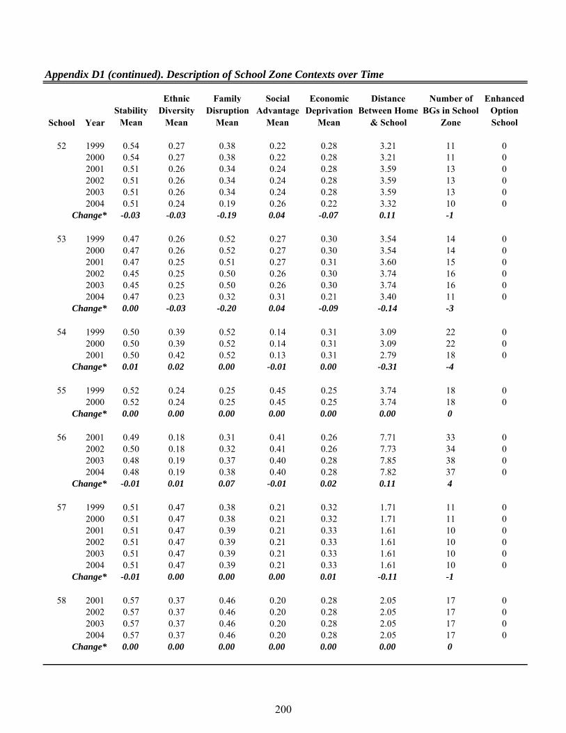
Appendix D1 (continued). Description of School Zone Contexts over Time

School YearStability

Mean

Ethnic Diversity

Mean

Family Disruption

Mean

Social Advantage

Mean

Economic Deprivation

Mean

Distance Between Home

& School

Number of BGs in School

Zone

Enhanced Option School

24 1999 0.57 0.37 0.48 0.21 0.28 1.92 14 02000 0.57 0.37 0.48 0.21 0.28 1.92 14 02001 0.57 0.37 0.46 0.20 0.28 2.05 17 02002 0.57 0.37 0.46 0.20 0.28 2.05 17 02003 0.51 0.38 0.46 0.17 0.32 2.60 24 02004 0.51 0.38 0.46 0.17 0.32 2.60 24 0

Change* -0.05 0.02 -0.02 -0.04 0.04 0.69 10

25 1999 0.62 0.24 0.39 0.29 0.23 5.96 16 02000 0.62 0.24 0.39 0.29 0.23 5.96 16 02001 0.65 0.23 0.41 0.29 0.24 4.09 15 02002 0.69 0.23 0.41 0.29 0.24 4.09 15 02003 0.69 0.23 0.41 0.29 0.24 4.09 15 02004 0.69 0.27 0.33 0.30 0.22 4.03 12 0

Change* 0.08 0.03 -0.06 0.01 -0.02 -1.93 -4

26 2001 0.40 0.25 0.43 0.28 0.32 4.37 20 02002 0.39 0.26 0.43 0.27 0.31 4.48 22 02003 0.39 0.26 0.43 0.27 0.31 4.48 22 02004 0.39 0.26 0.43 0.27 0.31 4.48 22 0

Change* -0.01 0.01 0.00 -0.01 -0.01 0.11 2

27 1999 0.45 0.23 0.45 0.17 0.32 3.92 20 02000 0.44 0.24 0.31 0.21 0.27 3.80 14 02001 0.44 0.24 0.31 0.21 0.27 3.80 14 02002 0.44 0.24 0.31 0.21 0.26 3.70 13 02003 0.44 0.24 0.31 0.21 0.26 3.70 13 02004 0.44 0.24 0.31 0.21 0.26 3.70 13 0

Change* -0.01 0.01 -0.13 0.03 -0.05 -0.22 -7

28 1999 0.42 0.29 0.41 0.20 0.30 4.59 25 02000 0.40 0.27 0.28 0.28 0.27 5.12 29 02001 0.40 0.27 0.28 0.28 0.27 5.12 29 02002 0.42 0.23 0.24 0.30 0.25 4.98 24 02003 0.42 0.23 0.24 0.30 0.25 4.98 24 02004 0.42 0.23 0.24 0.30 0.25 4.98 24 0

Change* 0.00 -0.06 -0.16 0.10 -0.05 0.38 -1

29 1999 0.44 0.22 0.28 0.31 0.23 6.24 36 02000 0.41 0.24 0.40 0.25 0.24 4.72 19 02001 0.42 0.24 0.40 0.24 0.25 4.69 18 02002 0.43 0.23 0.38 0.27 0.24 4.72 19 02003 0.41 0.27 0.24 0.30 0.18 4.77 15 02004 0.39 0.26 0.27 0.29 0.20 4.78 15 0

Change* -0.04 0.05 -0.01 -0.02 -0.03 -1.46 -21

195

Appendix D1 (continued). Description of School Zone Contexts over Time

School YearStability

Mean

Ethnic Diversity

Mean

Family Disruption

Mean

Social Advantage

Mean

Economic Deprivation

Mean

Distance Between Home

& School

Number of BGs in School

Zone

Enhanced Option School

30 1999 0.26 0.31 0.25 0.50 0.30 3.24 25 02000 0.26 0.31 0.25 0.50 0.30 3.24 25 02001 0.30 0.27 0.23 0.52 0.31 3.70 36 02002 0.27 0.28 0.26 0.46 0.31 4.10 46 02003 0.27 0.28 0.28 0.44 0.30 4.26 52 02004 0.27 0.28 0.29 0.43 0.31 4.29 53 0

Change* 0.01 -0.04 0.04 -0.07 0.01 1.05 28

31 1999 0.48 0.18 0.35 0.36 0.27 7.32 26 02000 0.48 0.18 0.35 0.36 0.27 7.32 26 02001 0.52 0.11 0.68 0.16 0.44 1.97 10 0

Change* 0.04 -0.06 0.32 -0.21 0.16 -5.35 -16

32 1999 0.45 0.38 0.50 0.19 0.35 3.32 42 02000 0.45 0.37 0.50 0.20 0.35 3.27 41 02001 0.44 0.38 0.50 0.20 0.35 3.05 37 02002 0.43 0.36 0.51 0.21 0.35 2.84 33 0

Change* -0.02 -0.02 0.01 0.01 0.01 -0.48 -9

33 1999 0.39 0.49 0.53 0.17 0.38 2.04 10 02000 0.39 0.49 0.53 0.17 0.38 2.04 10 02001 0.39 0.49 0.53 0.17 0.38 2.04 10 02002 0.47 0.47 0.66 0.13 0.34 1.67 8 12003 0.45 0.40 0.56 0.15 0.29 2.41 13 12004 0.45 0.39 0.55 0.12 0.30 2.34 12 1

Change* 0.06 -0.10 0.02 -0.04 -0.09 0.30 2

34 1999 0.35 0.39 0.28 0.32 0.22 6.06 14 02000 0.35 0.39 0.28 0.32 0.22 6.06 14 02001 0.36 0.41 0.23 0.34 0.18 6.06 13 02002 0.39 0.39 0.23 0.33 0.20 3.91 8 02003 0.39 0.39 0.23 0.33 0.20 3.91 8 02004 0.39 0.39 0.23 0.33 0.20 3.91 8 0

Change* 0.03 0.00 -0.05 0.02 -0.02 -2.15 -6

35 1999 0.51 0.22 0.44 0.26 0.25 3.35 11 02000 0.45 0.29 0.35 0.25 0.22 2.74 7 02001 0.37 0.30 0.33 0.25 0.23 2.52 5 02002 0.37 0.30 0.33 0.25 0.23 2.52 5 02003 0.37 0.30 0.33 0.25 0.23 2.52 5 02004 0.37 0.30 0.33 0.25 0.23 2.52 5 0

Change* -0.14 0.08 -0.10 0.00 -0.02 -0.83 -6

196

Appendix D1 (continued). Description of School Zone Contexts over Time

School YearStability

Mean

Ethnic Diversity

Mean

Family Disruption

Mean

Social Advantage

Mean

Economic Deprivation

Mean

Distance Between Home

& School

Number of BGs in School

Zone

Enhanced Option School

36 1999 0.43 0.31 0.32 0.25 0.22 3.01 25 02000 0.43 0.31 0.32 0.25 0.22 3.01 25 02001 0.43 0.31 0.32 0.25 0.22 3.01 25 02002 0.43 0.31 0.32 0.26 0.22 2.98 24 02003 0.41 0.29 0.28 0.25 0.22 2.54 18 02004 0.41 0.29 0.28 0.25 0.22 2.54 18 0

Change* -0.02 -0.02 -0.03 0.00 0.00 -0.46 -7

37 1999 0.50 0.23 0.21 0.48 0.19 6.35 26 02000 0.50 0.23 0.22 0.45 0.19 8.14 29 02001 0.50 0.23 0.22 0.45 0.19 8.14 29 02002 0.49 0.24 0.24 0.45 0.19 1.46 32 02003 0.49 0.24 0.24 0.45 0.19 8.27 32 0

Change* -0.01 0.01 0.03 -0.03 0.00 1.92 6

38 1999 0.42 0.42 0.38 0.21 0.29 3.07 8 02000 0.42 0.42 0.38 0.21 0.29 3.07 8 02001 0.39 0.49 0.30 0.21 0.23 3.30 9 02002 0.39 0.49 0.30 0.21 0.23 1.10 9 02003 0.39 0.49 0.30 0.21 0.23 3.30 9 02004 0.39 0.49 0.30 0.21 0.23 3.30 9 0

Change* -0.03 0.07 -0.08 0.00 -0.06 0.24 1

39 1999 0.49 0.27 0.45 0.16 0.30 4.25 20 02000 0.49 0.25 0.76 0.10 0.41 1.06 7 12001 0.50 0.15 0.80 0.11 0.42 0.82 5 12002 0.50 0.20 0.68 0.11 0.41 1.49 7 12003 0.50 0.20 0.68 0.11 0.41 1.49 7 12004 0.50 0.20 0.68 0.11 0.41 1.49 7 1

Change* 0.01 -0.07 0.23 -0.04 0.11 -2.77 -13

40 1999 0.30 0.46 0.40 0.22 0.26 3.98 13 02000 0.30 0.46 0.40 0.22 0.26 3.98 13 02001 0.23 0.55 0.34 0.23 0.20 3.54 9 02002 0.23 0.55 0.34 0.23 0.20 3.54 9 02003 0.23 0.55 0.34 0.23 0.20 3.54 9 02004 0.23 0.55 0.34 0.23 0.20 3.54 9 0

Change* -0.06 0.09 -0.07 0.01 -0.06 -0.44 -4

197

Appendix D1 (continued). Description of School Zone Contexts over Time

School YearStability

Mean

Ethnic Diversity

Mean

Family Disruption

Mean

Social Advantage

Mean

Economic Deprivation

Mean

Distance Between Home

& School

Number of BGs in School

Zone

Enhanced Option School

41 1999 0.48 0.27 0.40 0.22 0.24 5.55 13 02000 0.49 0.25 0.38 0.23 0.24 6.14 14 02001 0.51 0.21 0.30 0.24 0.25 5.99 12 02002 0.51 0.21 0.30 0.24 0.25 5.99 12 02003 0.51 0.21 0.30 0.24 0.25 5.99 12 02004 0.51 0.21 0.30 0.24 0.25 5.99 12 0

Change* 0.03 -0.06 -0.10 0.02 0.01 0.44 -1

42 1999 0.53 0.26 0.36 0.27 0.24 7.27 24 02000 0.52 0.29 0.31 0.27 0.23 7.02 20 02001 0.51 0.30 0.34 0.26 0.24 7.10 22 02002 0.50 0.29 0.34 0.26 0.25 7.76 21 02003 0.50 0.29 0.34 0.26 0.25 7.76 21 02004 0.50 0.29 0.34 0.26 0.25 7.76 21 0

Change* -0.03 0.03 -0.02 -0.01 0.01 0.48 -3

43 1999 0.43 0.20 0.31 0.40 0.24 6.92 14 02000 0.43 0.20 0.31 0.40 0.24 6.92 14 02001 0.43 0.20 0.31 0.40 0.24 6.92 14 02002 0.41 0.20 0.33 0.41 0.23 7.04 17 02003 0.41 0.20 0.33 0.41 0.23 7.04 17 02004 0.41 0.21 0.33 0.42 0.22 7.01 16 0

Change* -0.02 0.01 0.02 0.02 -0.02 0.10 2

44 1999 0.50 0.42 0.45 0.17 0.28 2.46 10 02000 0.50 0.42 0.45 0.17 0.28 2.46 10 02001 0.51 0.41 0.47 0.18 0.28 2.56 13 02002 0.50 0.41 0.43 0.19 0.29 3.82 31 02003 0.50 0.41 0.43 0.19 0.29 3.82 31 02004 0.49 0.38 0.50 0.17 0.31 3.94 37 0

Change* -0.02 -0.04 0.04 0.00 0.03 1.47 27

45 1999 0.50 0.23 0.21 0.48 0.19 6.35 26 02000 0.50 0.23 0.22 0.45 0.19 8.14 29 02001 0.50 0.23 0.22 0.45 0.19 8.14 29 02002 0.49 0.23 0.23 0.45 0.19 8.25 30 02003 0.49 0.23 0.23 0.45 0.19 8.25 30 02004 0.47 0.25 0.24 0.43 0.18 7.87 27 0

Change* -0.03 0.02 0.03 -0.05 -0.01 1.52 1

198

Appendix D1 (continued). Description of School Zone Contexts over Time

School YearStability

Mean

Ethnic Diversity

Mean

Family Disruption

Mean

Social Advantage

Mean

Economic Deprivation

Mean

Distance Between Home

& School

Number of BGs in School

Zone

Enhanced Option School

46 1999 0.55 0.34 0.44 0.24 0.27 5.92 9 02000 0.59 0.27 0.46 0.25 0.27 6.07 12 02001 0.59 0.27 0.46 0.25 0.27 6.07 12 02002 0.52 0.29 0.49 0.25 0.27 5.95 16 02003 0.52 0.29 0.49 0.25 0.27 5.95 16 02004 0.53 0.31 0.52 0.23 0.29 5.63 14 0

Change* -0.02 -0.04 0.07 -0.01 0.02 -0.29 5

47 1999 0.45 0.16 0.23 0.57 0.23 6.43 45 02000 0.45 0.16 0.23 0.57 0.23 6.43 45 02001 0.46 0.16 0.24 0.56 0.24 6.33 40 02002 0.46 0.16 0.25 0.55 0.24 6.33 41 02003 0.47 0.16 0.24 0.56 0.24 6.33 39 02004 0.47 0.16 0.24 0.56 0.24 6.33 39 0

Change* 0.03 0.01 0.01 -0.01 0.01 -0.10 -6

48 1999 0.34 0.25 0.29 0.45 0.30 6.95 29 02000 0.34 0.25 0.29 0.45 0.30 6.95 29 02001 0.41 0.21 0.25 0.49 0.18 6.62 14 02002 0.44 0.16 0.18 0.52 0.18 6.43 11 02003 0.45 0.15 0.17 0.52 0.18 6.06 10 02004 0.48 0.14 0.36 0.42 0.26 6.25 13 0

Change* 0.15 -0.11 0.07 -0.03 -0.03 -0.70 -16

49 1999 0.47 0.32 0.43 0.23 0.28 4.50 27 02000 0.45 0.33 0.44 0.22 0.28 4.48 26 02001 0.45 0.33 0.44 0.22 0.28 4.48 26 02002 0.50 0.27 0.53 0.23 0.31 3.25 12 02003 0.50 0.27 0.53 0.23 0.31 3.25 12 0

Change* 0.03 -0.05 0.10 0.01 0.04 -1.25 -15

50 1999 0.42 0.47 0.37 0.22 0.27 2.72 18 02000 0.42 0.47 0.37 0.22 0.27 2.72 18 02001 0.42 0.47 0.37 0.22 0.27 2.72 18 02002 0.42 0.47 0.37 0.22 0.27 2.72 18 02003 0.42 0.47 0.37 0.22 0.27 2.72 18 02004 0.41 0.50 0.30 0.24 0.23 2.58 15 0

Change* -0.01 0.03 -0.07 0.02 -0.04 -0.13 -3

51 1999 0.41 0.21 0.31 0.43 0.27 9.44 67 0Change* 0.00 0.00 0.00 0.00 0.00 0.00 0

199

Appendix D1 (continued). Description of School Zone Contexts over Time

School YearStability

Mean

Ethnic Diversity

Mean

Family Disruption

Mean

Social Advantage

Mean

Economic Deprivation

Mean

Distance Between Home

& School

Number of BGs in School

Zone

Enhanced Option School

52 1999 0.54 0.27 0.38 0.22 0.28 3.21 11 02000 0.54 0.27 0.38 0.22 0.28 3.21 11 02001 0.51 0.26 0.34 0.24 0.28 3.59 13 02002 0.51 0.26 0.34 0.24 0.28 3.59 13 02003 0.51 0.26 0.34 0.24 0.28 3.59 13 02004 0.51 0.24 0.19 0.26 0.22 3.32 10 0

Change* -0.03 -0.03 -0.19 0.04 -0.07 0.11 -1

53 1999 0.47 0.26 0.52 0.27 0.30 3.54 14 02000 0.47 0.26 0.52 0.27 0.30 3.54 14 02001 0.47 0.25 0.51 0.27 0.31 3.60 15 02002 0.45 0.25 0.50 0.26 0.30 3.74 16 02003 0.45 0.25 0.50 0.26 0.30 3.74 16 02004 0.47 0.23 0.32 0.31 0.21 3.40 11 0

Change* 0.00 -0.03 -0.20 0.04 -0.09 -0.14 -3

54 1999 0.50 0.39 0.52 0.14 0.31 3.09 22 02000 0.50 0.39 0.52 0.14 0.31 3.09 22 02001 0.50 0.42 0.52 0.13 0.31 2.79 18 0

Change* 0.01 0.02 0.00 -0.01 0.00 -0.31 -4

55 1999 0.52 0.24 0.25 0.45 0.25 3.74 18 02000 0.52 0.24 0.25 0.45 0.25 3.74 18 0

Change* 0.00 0.00 0.00 0.00 0.00 0.00 0

56 2001 0.49 0.18 0.31 0.41 0.26 7.71 33 02002 0.50 0.18 0.32 0.41 0.26 7.73 34 02003 0.48 0.19 0.37 0.40 0.28 7.85 38 02004 0.48 0.19 0.38 0.40 0.28 7.82 37 0

Change* -0.01 0.01 0.07 -0.01 0.02 0.11 4

57 1999 0.51 0.47 0.38 0.21 0.32 1.71 11 02000 0.51 0.47 0.38 0.21 0.32 1.71 11 02001 0.51 0.47 0.39 0.21 0.33 1.61 10 02002 0.51 0.47 0.39 0.21 0.33 1.61 10 02003 0.51 0.47 0.39 0.21 0.33 1.61 10 02004 0.51 0.47 0.39 0.21 0.33 1.61 10 0

Change* -0.01 0.00 0.00 0.00 0.01 -0.11 -1

58 2001 0.57 0.37 0.46 0.20 0.28 2.05 17 02002 0.57 0.37 0.46 0.20 0.28 2.05 17 02003 0.57 0.37 0.46 0.20 0.28 2.05 17 02004 0.57 0.37 0.46 0.20 0.28 2.05 17 0

Change* 0.00 0.00 0.00 0.00 0.00 0.00 0

200

Appendix D1 (continued). Description of School Zone Contexts over Time

School YearStability

Mean

Ethnic Diversity

Mean

Family Disruption

Mean

Social Advantage

Mean

Economic Deprivation

Mean

Distance Between Home

& School

Number of BGs in School

Zone

Enhanced Option School

59 1999 0.42 0.20 0.32 0.33 0.29 3.85 16 02000 0.42 0.20 0.32 0.33 0.29 3.85 16 02001 0.42 0.20 0.32 0.33 0.29 3.85 16 02002 0.44 0.19 0.30 0.35 0.28 4.07 18 02003 0.44 0.19 0.30 0.35 0.28 4.07 18 02004 0.42 0.19 0.15 0.41 0.22 3.77 14 0

Change* 0.00 -0.01 -0.17 0.08 -0.06 -0.09 -2

60 1999 0.69 0.18 0.31 0.24 0.26 7.46 11 02000 0.57 0.23 0.40 0.24 0.27 8.05 19 02001 0.61 0.17 0.28 0.24 0.25 10.23 15 02002 0.59 0.21 0.30 0.22 0.27 10.25 17 02003 0.59 0.21 0.30 0.22 0.27 10.25 17 02004 0.59 0.21 0.30 0.22 0.27 10.25 17 0

Change* -0.10 0.03 -0.01 -0.02 0.01 2.79 6

61 1999 0.66 0.25 0.33 0.24 0.29 10.82 23 02000 0.63 0.25 0.35 0.23 0.29 11.59 27 02001 0.60 0.25 0.35 0.24 0.28 11.84 32 02002 0.60 0.25 0.37 0.24 0.29 11.58 32 02003 0.63 0.24 0.35 0.23 0.29 11.58 28 02004 0.63 0.24 0.35 0.23 0.29 11.58 28 0

Change* -0.03 -0.01 0.01 -0.01 0.00 0.77 5

62 1999 0.51 0.51 0.58 0.09 0.33 1.64 8 02000 0.51 0.51 0.58 0.09 0.33 1.64 8 02001 0.51 0.51 0.58 0.09 0.33 1.64 8 02002 0.51 0.51 0.58 0.09 0.33 1.64 8 02003 0.51 0.51 0.58 0.09 0.33 1.64 8 02004 0.51 0.51 0.58 0.09 0.33 1.64 8 0

Change* 0.00 0.00 0.00 0.00 0.00 0.00 0

63 2002 0.38 0.44 0.24 0.35 0.16 7.00 16 02003 0.38 0.44 0.24 0.35 0.16 7.00 16 02004 0.38 0.44 0.24 0.35 0.16 7.00 16 0

Change* 0.00 0.00 0.00 0.00 0.00 0.00 0

64 1999 0.63 0.24 0.34 0.25 0.26 11.26 21 02000 0.55 0.34 0.44 0.24 0.27 5.92 9 02001 0.55 0.34 0.44 0.24 0.27 5.92 9 0

Change* -0.08 0.10 0.10 -0.01 0.01 -5.34 -12

201

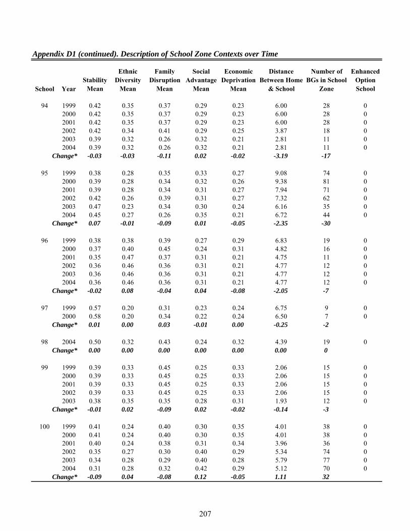
Appendix D1 (continued). Description of School Zone Contexts over Time

School YearStability

Mean

Ethnic Diversity

Mean

Family Disruption

Mean

Social Advantage

Mean

Economic Deprivation

Mean

Distance Between Home

& School

Number of BGs in School

Zone

Enhanced Option School

65 1999 0.37 0.42 0.46 0.11 0.43 1.61 7 02000 0.37 0.42 0.46 0.11 0.43 1.61 7 02001 0.37 0.42 0.46 0.11 0.43 1.61 7 02002 0.37 0.42 0.46 0.11 0.43 1.61 7 02003 0.37 0.42 0.46 0.11 0.43 1.61 7 02004 0.37 0.42 0.46 0.11 0.43 1.61 7 0

Change* 0.00 0.00 0.00 0.00 0.00 0.00 0

66 1999 0.53 0.35 0.50 0.19 0.31 3.41 34 02000 0.53 0.35 0.50 0.19 0.31 3.41 34 02001 0.51 0.36 0.49 0.19 0.31 3.46 36 02002 0.53 0.38 0.46 0.20 0.29 3.27 31 02003 0.53 0.39 0.45 0.22 0.27 2.99 26 02004 0.53 0.39 0.45 0.22 0.27 2.99 26 0

Change* 0.01 0.04 -0.05 0.03 -0.04 -0.41 -8

67 1999 0.38 0.36 0.47 0.22 0.35 2.13 18 02000 0.38 0.36 0.47 0.22 0.35 2.13 18 02001 0.38 0.36 0.47 0.22 0.35 2.13 18 02004 0.38 0.35 0.35 0.28 0.31 1.93 12 0

Change* -0.01 -0.01 -0.11 0.06 -0.05 -0.20 -6

68 1999 0.48 0.25 0.45 0.10 0.39 2.74 10 02000 0.51 0.21 0.48 0.10 0.41 2.71 9 02001 0.56 0.26 0.40 0.09 0.38 2.65 7 0

Change* 0.08 0.00 -0.05 0.00 -0.01 -0.09 -3

69 1999 0.39 0.26 0.41 0.27 0.27 4.59 28 02000 0.39 0.26 0.41 0.27 0.27 4.59 28 02001 0.41 0.23 0.45 0.25 0.29 4.50 27 02002 0.39 0.23 0.48 0.27 0.29 3.99 21 02003 0.45 0.23 0.45 0.27 0.26 3.46 15 02004 0.42 0.25 0.31 0.33 0.19 3.37 11 0

Change* 0.03 -0.01 -0.10 0.06 -0.08 -1.21 -17

70 1999 0.51 0.23 0.45 0.15 0.35 3.40 24 02000 0.51 0.23 0.45 0.15 0.35 3.40 24 02001 0.54 0.20 0.47 0.17 0.36 3.30 19 02002 0.54 0.20 0.47 0.17 0.36 3.30 19 02003 0.54 0.20 0.47 0.17 0.36 3.30 19 0

Change* 0.03 -0.03 0.02 0.02 0.01 -0.10 -5

202

Appendix D1 (continued). Description of School Zone Contexts over Time

School YearStability

Mean

Ethnic Diversity

Mean

Family Disruption

Mean

Social Advantage

Mean

Economic Deprivation

Mean

Distance Between Home

& School

Number of BGs in School

Zone

Enhanced Option School

71 1999 0.49 0.30 0.32 0.36 0.23 6.97 50 02000 0.49 0.30 0.31 0.35 0.23 8.62 53 02001 0.49 0.29 0.31 0.35 0.23 8.59 51 02002 0.48 0.29 0.32 0.36 0.23 8.61 52 02003 0.47 0.33 0.32 0.34 0.23 8.86 63 02004 0.46 0.33 0.31 0.33 0.22 8.69 58 0

Change* -0.03 0.03 -0.01 -0.03 -0.01 1.72 8

72 2002 0.32 0.42 0.29 0.32 0.18 6.14 11 02003 0.34 0.40 0.30 0.33 0.18 6.14 12 02004 0.34 0.40 0.30 0.33 0.18 6.14 11 0

Change* 0.02 -0.03 0.01 0.01 0.00 0.00 0

73 1999 0.52 0.36 0.44 0.21 0.28 2.23 18 02000 0.52 0.36 0.44 0.21 0.28 2.23 18 02001 0.51 0.35 0.44 0.22 0.27 2.20 17 02002 0.51 0.35 0.43 0.22 0.27 2.15 16 02003 0.51 0.35 0.43 0.22 0.27 2.15 16 02004 0.51 0.35 0.43 0.22 0.27 2.15 16 0

Change* -0.01 -0.01 -0.01 0.01 -0.01 -0.08 -2

74 1999 0.44 0.21 0.23 0.53 0.25 10.16 96 02000 0.44 0.21 0.23 0.53 0.25 10.16 96 02001 0.44 0.21 0.23 0.54 0.24 10.14 95 02002 0.49 0.19 0.24 0.52 0.23 9.64 72 02003 0.49 0.19 0.23 0.53 0.23 9.56 70 02004 0.50 0.19 0.25 0.54 0.23 9.28 66 0

Change* 0.06 -0.03 0.02 0.01 -0.02 -0.88 -30

75 1999 0.68 0.19 0.19 0.27 0.23 8.56 7 02000 0.68 0.19 0.19 0.27 0.23 8.56 7 0

Change* 0.00 0.00 0.00 0.00 0.00 0.00 0

76 2000 0.31 0.46 0.23 0.36 0.15 6.53 8 02001 0.31 0.46 0.23 0.36 0.15 6.53 8 02002 0.31 0.46 0.23 0.36 0.15 6.53 8 02003 0.31 0.46 0.23 0.36 0.15 6.53 8 02004 0.31 0.46 0.23 0.36 0.15 6.53 8 0

Change* 0.00 0.00 0.00 0.00 0.00 0.00 0

203

Appendix D1 (continued). Description of School Zone Contexts over Time

School YearStability

Mean

Ethnic Diversity

Mean

Family Disruption

Mean

Social Advantage

Mean

Economic Deprivation

Mean

Distance Between Home

& School

Number of BGs in School

Zone

Enhanced Option School

77 1999 0.40 0.42 0.30 0.29 0.21 8.24 46 02000 0.38 0.43 0.31 0.29 0.21 8.81 36 02001 0.38 0.45 0.30 0.29 0.21 8.02 34 02002 0.39 0.46 0.30 0.28 0.22 7.56 32 02003 0.37 0.42 0.31 0.32 0.21 5.77 17 02004 0.37 0.42 0.31 0.32 0.21 5.77 17 0

Change* -0.03 0.00 0.00 0.03 0.00 -2.47 -29

78 2001 0.37 0.21 0.72 0.11 0.61 0.77 5 12002 0.37 0.21 0.72 0.11 0.61 0.77 6 12003 0.37 0.21 0.72 0.11 0.61 0.77 6 12004 0.37 0.21 0.72 0.11 0.61 0.77 6 1

Change* 0.00 0.00 0.00 0.00 0.00 0.00 1

79 1999 0.51 0.33 0.40 0.17 0.27 3.13 10 02000 0.51 0.33 0.40 0.17 0.27 3.13 10 02001 0.46 0.37 0.32 0.18 0.25 2.96 7 02002 0.46 0.37 0.32 0.18 0.25 2.96 7 02003 0.46 0.37 0.32 0.18 0.25 2.96 7 02004 0.46 0.37 0.32 0.18 0.25 2.96 7 0

Change* -0.05 0.04 -0.07 0.01 -0.02 -0.17 -3

80 1999 0.44 0.33 0.39 0.19 0.27 5.24 32 02000 0.44 0.33 0.39 0.19 0.27 5.24 32 02001 0.44 0.33 0.37 0.19 0.27 4.90 29 02002 0.42 0.34 0.35 0.19 0.25 4.50 23 02003 0.42 0.34 0.35 0.19 0.25 4.50 23 02004 0.42 0.34 0.35 0.19 0.25 4.50 23 0

Change* -0.02 0.01 -0.04 0.00 -0.01 -0.74 -9

81 1999 0.55 0.28 0.31 0.31 0.22 5.38 9 02000 0.55 0.28 0.31 0.31 0.22 5.38 9 02001 0.55 0.26 0.40 0.28 0.24 5.66 12 02002 0.50 0.31 0.43 0.25 0.24 5.62 14 02003 0.50 0.31 0.43 0.25 0.24 5.62 14 02004 0.50 0.31 0.43 0.25 0.24 5.62 14 0

Change* -0.05 0.04 0.12 -0.06 0.02 0.24 5

82 1999 0.42 0.48 0.35 0.20 0.31 2.79 15 02000 0.42 0.48 0.35 0.20 0.31 2.79 15 02001 0.41 0.53 0.27 0.21 0.24 1.99 9 02002 0.41 0.53 0.27 0.21 0.24 1.99 9 02003 0.41 0.53 0.27 0.21 0.24 1.99 9 02004 0.41 0.53 0.27 0.21 0.24 1.99 9 0

Change* 0.00 0.05 -0.07 0.01 -0.06 -0.81 -6

204

Appendix D1 (continued). Description of School Zone Contexts over Time

School YearStability

Mean

Ethnic Diversity

Mean

Family Disruption

Mean

Social Advantage

Mean

Economic Deprivation

Mean

Distance Between Home

& School

Number of BGs in School

Zone

Enhanced Option School

83 1999 0.44 0.39 0.54 0.27 0.26 0.89 4 02000 0.44 0.39 0.54 0.27 0.26 0.89 4 12001 0.42 0.30 0.58 0.23 0.38 1.76 11 12002 0.43 0.27 0.60 0.24 0.40 1.68 10 12003 0.42 0.23 0.66 0.22 0.43 1.80 12 12004 0.42 0.23 0.66 0.22 0.43 1.80 12 1

Change* -0.02 -0.16 0.12 -0.05 0.16 0.91 8

84 1999 0.52 0.19 0.25 0.39 0.22 4.55 17 02000 0.52 0.19 0.25 0.39 0.22 4.55 17 02001 0.52 0.19 0.25 0.39 0.22 4.55 17 02002 0.52 0.19 0.25 0.39 0.22 4.55 17 02003 0.47 0.21 0.27 0.42 0.23 4.35 13 02004 0.53 0.15 0.14 0.42 0.19 4.25 11 0

Change* 0.01 -0.04 -0.11 0.03 -0.03 -0.30 -6

85 1999 0.51 0.20 0.22 0.55 0.22 7.65 35 02000 0.51 0.20 0.22 0.55 0.22 7.65 35 02001 0.51 0.20 0.22 0.55 0.22 7.65 35 02002 0.51 0.20 0.22 0.55 0.22 7.65 35 02003 0.51 0.20 0.22 0.55 0.22 7.65 35 02004 0.51 0.20 0.22 0.55 0.22 7.71 36 0

Change* 0.00 0.00 -0.01 0.00 0.00 0.06 1

86 1999 0.60 0.45 0.49 0.21 0.28 2.04 9 02000 0.60 0.45 0.49 0.21 0.28 2.04 9 02001 0.57 0.46 0.48 0.21 0.27 2.08 10 02002 0.57 0.46 0.48 0.21 0.27 2.08 10 02003 0.57 0.46 0.48 0.21 0.27 2.08 10 02004 0.57 0.46 0.48 0.21 0.27 2.08 10 0

Change* -0.03 0.01 -0.01 0.00 -0.01 0.04 1

87 1999 0.45 0.35 0.35 0.30 0.24 6.93 56 02000 0.46 0.35 0.35 0.30 0.25 6.32 51 02001 0.43 0.35 0.34 0.30 0.27 5.25 53 02002 0.46 0.36 0.35 0.30 0.25 4.98 48 02003 0.46 0.36 0.35 0.30 0.25 4.98 48 0

Change* 0.01 0.00 0.01 0.00 0.01 -1.94 -8

205

Appendix D1 (continued). Description of School Zone Contexts over Time

School YearStability

Mean

Ethnic Diversity

Mean

Family Disruption

Mean

Social Advantage

Mean

Economic Deprivation

Mean

Distance Between Home

& School

Number of BGs in School

Zone

Enhanced Option School

88 1999 0.46 0.36 0.46 0.31 0.29 1.25 9 02000 0.46 0.36 0.46 0.31 0.29 1.25 9 02001 0.46 0.36 0.46 0.31 0.29 1.25 9 02002 0.46 0.36 0.46 0.31 0.29 1.25 9 02003 0.46 0.36 0.46 0.31 0.29 1.25 9 02004 0.46 0.35 0.42 0.32 0.28 1.32 10 0

Change* 0.00 -0.01 -0.04 0.01 0.00 0.07 1

89 1999 0.49 0.29 0.52 0.17 0.30 1.81 8 02000 0.49 0.29 0.52 0.17 0.30 1.81 8 02001 0.52 0.30 0.55 0.16 0.32 1.93 10 02002 0.52 0.30 0.55 0.16 0.32 1.93 10 02003 0.52 0.30 0.55 0.16 0.32 1.93 10 02004 0.52 0.30 0.55 0.16 0.32 1.93 10 0

Change* 0.03 0.00 0.03 -0.01 0.01 0.11 2

90 1999 0.48 0.17 0.23 0.56 0.23 9.16 65 02000 0.48 0.17 0.23 0.56 0.23 9.16 65 02001 0.48 0.17 0.23 0.56 0.23 9.16 65 02002 0.49 0.17 0.24 0.55 0.23 8.89 62 0

Change* 0.01 0.00 0.01 -0.01 0.00 -0.27 -3

91 1999 0.36 0.30 0.51 0.14 0.33 2.92 16 02000 0.36 0.30 0.51 0.14 0.33 2.92 16 02001 0.40 0.31 0.47 0.17 0.30 3.37 20 02002 0.41 0.31 0.45 0.17 0.29 4.27 23 02003 0.41 0.31 0.45 0.17 0.29 4.27 23 02004 0.42 0.33 0.34 0.19 0.25 4.22 19 0

Change* 0.06 0.03 -0.17 0.05 -0.08 1.29 3

92 1999 0.39 0.15 0.43 0.40 0.30 2.35 20 02000 0.39 0.14 0.41 0.41 0.29 2.30 19 02001 0.39 0.14 0.42 0.40 0.30 2.22 18 02002 0.40 0.22 0.41 0.41 0.28 3.11 29 02003 0.40 0.21 0.41 0.44 0.26 3.11 27 02004 0.42 0.23 0.35 0.47 0.23 3.15 23 0

Change* 0.03 0.08 -0.08 0.07 -0.06 0.80 3

93 1999 0.38 0.28 0.42 0.25 0.24 4.06 13 02000 0.38 0.28 0.42 0.25 0.24 4.06 13 02001 0.38 0.28 0.42 0.25 0.24 4.06 13 02002 0.38 0.28 0.42 0.25 0.24 4.06 13 02003 0.38 0.28 0.42 0.25 0.24 4.06 13 02004 0.37 0.32 0.31 0.27 0.20 4.01 11 0

Change* -0.01 0.03 -0.10 0.03 -0.05 -0.05 -2

206

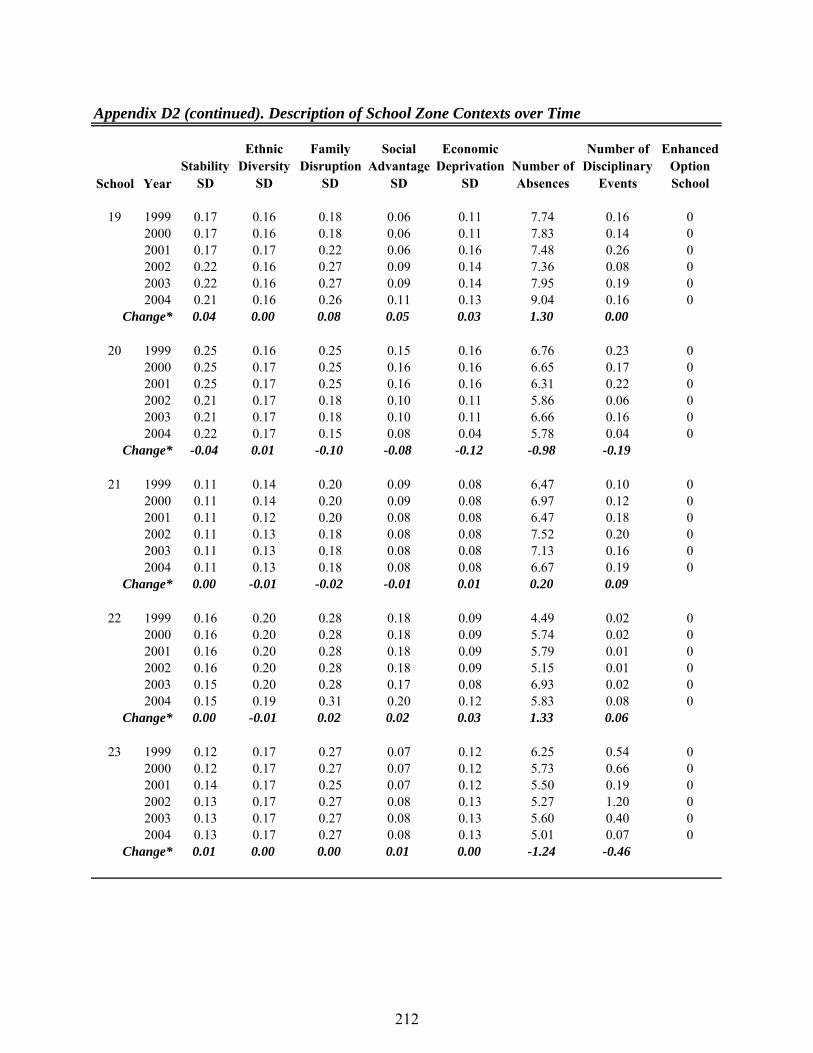
Appendix D1 (continued). Description of School Zone Contexts over Time

School YearStability

Mean

Ethnic Diversity

Mean

Family Disruption

Mean

Social Advantage

Mean

Economic Deprivation

Mean

Distance Between Home

& School

Number of BGs in School

Zone

Enhanced Option School

94 1999 0.42 0.35 0.37 0.29 0.23 6.00 28 02000 0.42 0.35 0.37 0.29 0.23 6.00 28 02001 0.42 0.35 0.37 0.29 0.23 6.00 28 02002 0.42 0.34 0.41 0.29 0.25 3.87 18 02003 0.39 0.32 0.26 0.32 0.21 2.81 11 02004 0.39 0.32 0.26 0.32 0.21 2.81 11 0

Change* -0.03 -0.03 -0.11 0.02 -0.02 -3.19 -17

95 1999 0.38 0.28 0.35 0.33 0.27 9.08 74 02000 0.39 0.28 0.34 0.32 0.26 9.38 81 02001 0.39 0.28 0.34 0.31 0.27 7.94 71 02002 0.42 0.26 0.39 0.31 0.27 7.32 62 02003 0.47 0.23 0.34 0.30 0.24 6.16 35 02004 0.45 0.27 0.26 0.35 0.21 6.72 44 0

Change* 0.07 -0.01 -0.09 0.01 -0.05 -2.35 -30

96 1999 0.38 0.38 0.39 0.27 0.29 6.83 19 02000 0.37 0.40 0.45 0.24 0.31 4.82 16 02001 0.35 0.47 0.37 0.31 0.21 4.75 11 02002 0.36 0.46 0.36 0.31 0.21 4.77 12 02003 0.36 0.46 0.36 0.31 0.21 4.77 12 02004 0.36 0.46 0.36 0.31 0.21 4.77 12 0

Change* -0.02 0.08 -0.04 0.04 -0.08 -2.05 -7

97 1999 0.57 0.20 0.31 0.23 0.24 6.75 9 02000 0.58 0.20 0.34 0.22 0.24 6.50 7 0

Change* 0.01 0.00 0.03 -0.01 0.00 -0.25 -2

98 2004 0.50 0.32 0.43 0.24 0.32 4.39 19 0Change* 0.00 0.00 0.00 0.00 0.00 0.00 0

99 1999 0.39 0.33 0.45 0.25 0.33 2.06 15 02000 0.39 0.33 0.45 0.25 0.33 2.06 15 02001 0.39 0.33 0.45 0.25 0.33 2.06 15 02002 0.39 0.33 0.45 0.25 0.33 2.06 15 02003 0.38 0.35 0.35 0.28 0.31 1.93 12 0

Change* -0.01 0.02 -0.09 0.02 -0.02 -0.14 -3

100 1999 0.41 0.24 0.40 0.30 0.35 4.01 38 02000 0.41 0.24 0.40 0.30 0.35 4.01 38 02001 0.40 0.24 0.38 0.31 0.34 3.96 36 02002 0.35 0.27 0.30 0.40 0.29 5.34 74 02003 0.34 0.28 0.29 0.40 0.28 5.79 77 02004 0.31 0.28 0.32 0.42 0.29 5.12 70 0

Change* -0.09 0.04 -0.08 0.12 -0.05 1.11 32

207

Appendix D1 (continued). Description of School Zone Contexts over Time

School YearStability

Mean

Ethnic Diversity

Mean

Family Disruption

Mean

Social Advantage

Mean

Economic Deprivation

Mean

Distance Between Home

& School

Number of BGs in School

Zone

Enhanced Option School

101 1999 0.38 0.21 0.40 0.41 0.25 6.40 18 02000 0.38 0.21 0.40 0.41 0.25 6.40 18 02001 0.38 0.21 0.40 0.41 0.25 6.40 18 02002 0.37 0.22 0.40 0.40 0.25 6.24 16 02003 0.37 0.22 0.40 0.40 0.25 6.24 16 02004 0.41 0.22 0.41 0.41 0.23 6.23 14 0

Change* 0.03 0.01 0.01 0.01 -0.01 -0.17 -4

102 1999 0.48 0.20 0.48 0.21 0.34 3.37 24 02000 0.48 0.20 0.48 0.21 0.34 3.37 24 02001 0.48 0.20 0.48 0.21 0.34 3.37 24 02002 0.46 0.22 0.56 0.17 0.41 3.45 26 02003 0.47 0.22 0.55 0.17 0.40 3.49 27 02004 0.47 0.22 0.53 0.17 0.38 3.70 32 0

Change* -0.01 0.02 0.05 -0.04 0.05 0.32 8

103 1999 0.48 0.44 0.25 0.16 0.26 2.12 9 02000 0.48 0.44 0.25 0.16 0.26 2.12 9 02001 0.42 0.38 0.37 0.20 0.34 2.47 16 02002 0.43 0.39 0.41 0.19 0.35 2.71 18 02003 0.43 0.39 0.41 0.19 0.35 2.71 18 02004 0.43 0.39 0.41 0.19 0.35 2.71 18 0

Change* -0.05 -0.05 0.16 0.03 0.09 0.59 9

104 1999 0.38 0.39 0.36 0.22 0.29 6.06 65 02000 0.38 0.39 0.36 0.22 0.29 6.06 65 02001 0.37 0.40 0.30 0.23 0.26 5.41 50 02002 0.41 0.38 0.32 0.22 0.24 4.66 38 02003 0.41 0.38 0.32 0.22 0.24 4.66 38 02004 0.41 0.38 0.32 0.22 0.24 4.66 38 0

Change* 0.03 -0.01 -0.04 0.00 -0.04 -1.40 -27

District Average 1999 0.465 0.305 0.382 0.274 0.278 4.867 22.946 ―

2000 0.462 0.309 0.386 0.272 0.278 4.710 21.645 ―2001 0.458 0.310 0.392 0.270 0.280 4.490 21.255 ―2002 0.457 0.316 0.386 0.276 0.273 4.460 21.098 ―2003 0.455 0.317 0.382 0.274 0.270 4.421 20.000 ―2004 0.453 0.319 0.379 0.274 0.269 4.345 19.207 ―

All Years 0.458 0.313 0.385 0.273 0.275 4.550 21.053 ―

Avg. Change* -0.012 0.014 -0.003 0.000 -0.010 -0.522 -3.739 ―

*Change is calculated by subtracting values from 2004 from the baseline values for 1999. When a school was not opened in 1999 or 2004, values for the latest year were subtracted from values in the earliest year.

208

Appendix D2. Description of School Zone Contexts over Time

School YearStability

SD

Ethnic Diversity

SD

Family Disruption

SD

Social Advantage

SD

Economic Deprivation

SDNumber of Absences

Number of Disciplinary

Events

Enhanced Option School

1 1999 0.17 0.20 0.32 0.26 0.21 8.33 0.43 02000 0.17 0.20 0.32 0.26 0.21 8.38 0.53 02001 0.22 0.20 0.32 0.23 0.17 7.60 0.27 02002 0.21 0.18 0.30 0.24 0.15 8.18 0.44 0

Change* 0.04 -0.02 -0.02 -0.02 -0.06 -0.14 0.00

2 1999 0.14 0.14 0.21 0.13 0.09 5.59 0.18 02000 0.14 0.14 0.21 0.13 0.09 5.55 0.11 02001 0.14 0.14 0.20 0.13 0.09 4.69 0.10 02002 0.14 0.11 0.20 0.06 0.09 5.61 0.00 02003 0.14 0.11 0.20 0.06 0.09 6.69 0.00 02004 0.14 0.11 0.20 0.06 0.09 7.36 0.01 0

Change* -0.01 -0.02 -0.01 -0.08 -0.01 1.77 -0.17

3 2000 0.20 0.17 0.12 0.10 0.04 7.87 0.98 02001 0.20 0.16 0.14 0.09 0.04 8.37 1.27 02002 0.20 0.16 0.14 0.08 0.04 7.73 1.20 02003 0.20 0.17 0.14 0.09 0.04 7.94 1.05 02004 0.20 0.17 0.14 0.09 0.04 7.94 2.23 0

Change* 0.00 0.00 0.02 -0.01 0.00 0.07 1.26

4 2002 0.15 0.13 0.31 0.15 0.15 9.83 2.77 02003 0.15 0.13 0.32 0.15 0.15 10.91 2.70 02004 0.15 0.13 0.32 0.15 0.15 11.94 1.96 0

Change* 0.00 0.00 0.00 0.00 -0.01 2.11 -0.81

5 1999 0.17 0.16 0.27 0.14 0.13 7.44 1.60 02000 0.17 0.16 0.27 0.14 0.13 7.59 0.88 02001 0.15 0.17 0.28 0.14 0.11 7.55 1.35 02002 0.11 0.18 0.23 0.09 0.07 9.85 1.00 02003 0.11 0.18 0.23 0.09 0.07 10.16 2.93 02004 0.12 0.18 0.28 0.09 0.10 10.88 3.22 0

Change* -0.04 0.03 0.01 -0.05 -0.03 3.44 1.63

6 1999 0.15 0.17 0.21 0.15 0.19 5.63 0.47 02000 0.14 0.16 0.22 0.13 0.20 6.17 0.70 02001 0.15 0.06 0.12 0.06 0.04 5.00 0.19 02002 0.13 0.05 0.12 0.07 0.04 5.78 0.05 02003 0.13 0.05 0.12 0.07 0.04 5.31 0.02 02004 0.13 0.05 0.12 0.07 0.04 5.22 0.04 0

Change* -0.02 -0.12 -0.09 -0.08 -0.15 -0.40 -0.44

209

Appendix D2 (continued). Description of School Zone Contexts over Time

School YearStability

SD

Ethnic Diversity

SD

Family Disruption

SD

Social Advantage

SD

Economic Deprivation

SDNumber of Absences

Number of Disciplinary

Events

Enhanced Option School

7 1999 0.19 0.17 0.30 0.22 0.13 10.74 1.55 02000 0.19 0.17 0.30 0.22 0.13 11.03 0.97 02001 0.16 0.17 0.33 0.21 0.13 9.21 0.86 02002 0.16 0.17 0.33 0.21 0.13 8.66 0.87 02003 0.15 0.17 0.37 0.22 0.15 9.09 0.61 02004 0.17 0.17 0.35 0.21 0.14 8.94 1.12 0

Change* -0.02 0.00 0.05 -0.01 0.01 -1.80 -0.43

8 1999 0.16 0.20 0.30 0.19 0.14 7.02 0.03 02000 0.16 0.20 0.30 0.19 0.14 7.34 0.04 02001 0.14 0.18 0.20 0.19 0.05 5.65 0.25 02002 0.14 0.17 0.19 0.17 0.05 4.92 1.68 02003 0.14 0.17 0.19 0.17 0.05 5.35 0.23 02004 0.14 0.17 0.19 0.17 0.05 5.39 0.09 0

Change* -0.02 -0.03 -0.12 -0.02 -0.09 -1.63 0.07

9 1999 0.12 0.19 0.27 0.17 0.13 6.23 0.11 02000 0.12 0.19 0.27 0.17 0.13 6.03 0.10 02001 0.12 0.19 0.27 0.17 0.13 7.45 0.15 02002 0.13 0.19 0.29 0.17 0.15 6.49 0.00 02003 0.12 0.17 0.26 0.15 0.13 6.25 0.07 02004 0.12 0.18 0.26 0.14 0.12 4.58 0.02 0

Change* 0.00 -0.02 -0.01 -0.03 -0.01 -1.65 -0.10

10 1999 0.12 0.18 0.22 0.05 0.12 6.66 0.67 02000 0.12 0.18 0.22 0.05 0.12 6.03 0.26 02001 0.12 0.18 0.22 0.05 0.12 7.54 0.22 02002 0.09 0.17 0.28 0.03 0.15 7.32 0.03 12003 0.09 0.17 0.28 0.03 0.15 6.48 1.39 12004 0.09 0.17 0.28 0.03 0.15 5.80 0.18 1

Change* -0.04 -0.01 0.06 -0.02 0.03 -0.86 -0.49

11 1999 0.16 0.16 0.24 0.10 0.05 7.40 1.55 02000 0.13 0.15 0.24 0.11 0.05 4.30 0.75 02001 0.13 0.14 0.25 0.11 0.05 6.19 0.88 02002 0.14 0.17 0.22 0.10 0.07 8.43 0.69 02003 0.14 0.17 0.22 0.10 0.07 8.78 0.99 02004 0.14 0.17 0.22 0.10 0.07 9.33 1.65 0

Change* -0.02 0.01 -0.02 0.00 0.02 1.93 0.10

210

Appendix D2 (continued). Description of School Zone Contexts over Time

School YearStability

SD

Ethnic Diversity

SD

Family Disruption

SD

Social Advantage

SD

Economic Deprivation

SDNumber of Absences

Number of Disciplinary

Events

Enhanced Option School

12 1999 0.15 0.17 0.22 0.11 0.06 9.91 3.40 02000 0.15 0.18 0.20 0.11 0.06 8.07 0.49 02001 0.16 0.17 0.21 0.11 0.06 7.90 0.77 02002 0.13 0.18 0.23 0.13 0.10 6.57 0.38 02003 0.14 0.18 0.23 0.12 0.10 8.39 2.05 02004 0.13 0.19 0.22 0.08 0.10 9.11 2.25 0

Change* -0.01 0.02 0.00 -0.03 0.04 -0.80 -1.15

13 1999 0.21 0.15 0.31 0.19 0.14 6.47 0.15 02000 0.21 0.15 0.31 0.19 0.14 6.96 0.18 02001 0.21 0.15 0.31 0.19 0.14 6.05 0.09 02002 0.20 0.16 0.29 0.21 0.12 7.01 0.05 02003 0.20 0.16 0.29 0.21 0.12 6.39 0.08 02004 0.20 0.18 0.32 0.21 0.13 6.75 0.06 0

Change* -0.01 0.02 0.01 0.02 -0.01 0.27 -0.08

14 2004 0.21 0.11 0.16 0.09 0.13 6.36 0.22 1Change* 0.00 0.00 0.00 0.00 0.00 0.00 0.00

15 1999 0.16 0.18 0.20 0.14 0.18 11.48 1.37 02000 0.15 0.18 0.21 0.15 0.19 10.97 1.56 02001 0.17 0.17 0.26 0.19 0.16 11.80 1.57 02002 0.16 0.18 0.28 0.18 0.15 12.76 1.76 02003 0.16 0.18 0.28 0.18 0.15 7.90 2.26 02004 0.16 0.18 0.28 0.18 0.15 7.96 1.28 0

Change* 0.01 0.00 0.07 0.04 -0.03 -3.52 -0.09

16 1999 0.24 0.16 0.23 0.14 0.15 7.67 0.69 0Change* 0.00 0.00 0.00 0.00 0.00 0.00 0.00

17 1999 0.17 0.15 0.32 0.11 0.13 6.28 0.14 02000 0.17 0.15 0.32 0.11 0.13 5.94 0.15 02001 0.15 0.16 0.30 0.11 0.11 5.59 0.08 02002 0.17 0.14 0.24 0.09 0.07 5.73 0.05 02003 0.17 0.14 0.24 0.09 0.07 8.46 0.01 02004 0.17 0.14 0.24 0.09 0.07 6.80 0.06 0

Change* 0.00 0.00 -0.08 -0.02 -0.06 0.52 -0.08

18 1999 0.23 0.16 0.33 0.10 0.16 10.73 0.19 02000 0.23 0.16 0.33 0.10 0.16 10.22 0.59 02001 0.23 0.16 0.33 0.10 0.16 7.15 0.08 02002 0.20 0.17 0.24 0.17 0.13 7.42 0.02 02003 0.20 0.17 0.24 0.17 0.13 8.10 0.01 02004 0.17 0.17 0.33 0.15 0.13 7.39 0.05 0

Change* -0.06 0.01 0.00 0.05 -0.03 -3.34 -0.14

211

Appendix D2 (continued). Description of School Zone Contexts over Time

School YearStability

SD

Ethnic Diversity

SD

Family Disruption

SD

Social Advantage

SD

Economic Deprivation

SDNumber of Absences

Number of Disciplinary

Events

Enhanced Option School

19 1999 0.17 0.16 0.18 0.06 0.11 7.74 0.16 02000 0.17 0.16 0.18 0.06 0.11 7.83 0.14 02001 0.17 0.17 0.22 0.06 0.16 7.48 0.26 02002 0.22 0.16 0.27 0.09 0.14 7.36 0.08 02003 0.22 0.16 0.27 0.09 0.14 7.95 0.19 02004 0.21 0.16 0.26 0.11 0.13 9.04 0.16 0

Change* 0.04 0.00 0.08 0.05 0.03 1.30 0.00

20 1999 0.25 0.16 0.25 0.15 0.16 6.76 0.23 02000 0.25 0.17 0.25 0.16 0.16 6.65 0.17 02001 0.25 0.17 0.25 0.16 0.16 6.31 0.22 02002 0.21 0.17 0.18 0.10 0.11 5.86 0.06 02003 0.21 0.17 0.18 0.10 0.11 6.66 0.16 02004 0.22 0.17 0.15 0.08 0.04 5.78 0.04 0

Change* -0.04 0.01 -0.10 -0.08 -0.12 -0.98 -0.19

21 1999 0.11 0.14 0.20 0.09 0.08 6.47 0.10 02000 0.11 0.14 0.20 0.09 0.08 6.97 0.12 02001 0.11 0.12 0.20 0.08 0.08 6.47 0.18 02002 0.11 0.13 0.18 0.08 0.08 7.52 0.20 02003 0.11 0.13 0.18 0.08 0.08 7.13 0.16 02004 0.11 0.13 0.18 0.08 0.08 6.67 0.19 0

Change* 0.00 -0.01 -0.02 -0.01 0.01 0.20 0.09

22 1999 0.16 0.20 0.28 0.18 0.09 4.49 0.02 02000 0.16 0.20 0.28 0.18 0.09 5.74 0.02 02001 0.16 0.20 0.28 0.18 0.09 5.79 0.01 02002 0.16 0.20 0.28 0.18 0.09 5.15 0.01 02003 0.15 0.20 0.28 0.17 0.08 6.93 0.02 02004 0.15 0.19 0.31 0.20 0.12 5.83 0.08 0

Change* 0.00 -0.01 0.02 0.02 0.03 1.33 0.06

23 1999 0.12 0.17 0.27 0.07 0.12 6.25 0.54 02000 0.12 0.17 0.27 0.07 0.12 5.73 0.66 02001 0.14 0.17 0.25 0.07 0.12 5.50 0.19 02002 0.13 0.17 0.27 0.08 0.13 5.27 1.20 02003 0.13 0.17 0.27 0.08 0.13 5.60 0.40 02004 0.13 0.17 0.27 0.08 0.13 5.01 0.07 0

Change* 0.01 0.00 0.00 0.01 0.00 -1.24 -0.46

212

Appendix D2 (continued). Description of School Zone Contexts over Time

School YearStability

SD

Ethnic Diversity

SD

Family Disruption

SD

Social Advantage

SD

Economic Deprivation

SDNumber of Absences

Number of Disciplinary

Events

Enhanced Option School

24 1999 0.10 0.15 0.24 0.07 0.12 6.05 0.13 02000 0.10 0.15 0.24 0.07 0.12 5.62 0.08 02001 0.10 0.15 0.22 0.07 0.12 6.40 0.45 02002 0.10 0.15 0.22 0.07 0.12 7.13 0.43 02003 0.14 0.14 0.26 0.09 0.15 10.70 0.88 02004 0.14 0.14 0.26 0.09 0.15 11.32 1.31 0

Change* 0.03 -0.01 0.02 0.03 0.03 5.27 1.18

25 1999 0.19 0.18 0.28 0.13 0.15 6.29 0.07 02000 0.19 0.18 0.28 0.13 0.15 7.12 0.18 02001 0.20 0.18 0.28 0.13 0.15 6.11 0.13 02002 0.20 0.18 0.28 0.13 0.15 6.77 0.09 02003 0.20 0.18 0.28 0.13 0.15 7.36 0.01 02004 0.17 0.17 0.19 0.15 0.15 6.46 0.01 0

Change* -0.02 -0.01 -0.10 0.02 0.01 0.16 -0.07

26 2001 0.17 0.17 0.23 0.16 0.20 10.70 0.61 02002 0.17 0.17 0.22 0.15 0.20 11.68 0.62 02003 0.17 0.17 0.22 0.15 0.20 10.60 3.03 02004 0.17 0.17 0.22 0.15 0.20 11.14 3.49 0

Change* 0.00 0.00 -0.01 0.00 0.00 0.44 2.88

27 1999 0.13 0.17 0.28 0.13 0.13 6.88 0.08 02000 0.12 0.17 0.19 0.15 0.10 5.95 0.11 02001 0.12 0.17 0.19 0.15 0.10 6.25 0.10 02002 0.12 0.17 0.20 0.15 0.11 7.07 0.07 02003 0.12 0.17 0.20 0.15 0.11 6.99 0.20 02004 0.12 0.17 0.20 0.15 0.11 5.89 0.04 0

Change* -0.01 0.01 -0.09 0.02 -0.02 -0.99 -0.04

28 1999 0.12 0.17 0.23 0.12 0.09 13.75 4.56 02000 0.12 0.18 0.21 0.19 0.11 10.79 1.19 02001 0.12 0.18 0.21 0.19 0.11 10.25 0.77 02002 0.12 0.17 0.18 0.21 0.10 8.98 0.64 02003 0.12 0.17 0.18 0.21 0.10 10.08 1.61 02004 0.12 0.17 0.18 0.21 0.10 9.58 1.88 0

Change* -0.01 0.00 -0.05 0.08 0.01 -4.17 -2.68

29 1999 0.16 0.15 0.26 0.17 0.12 9.35 2.24 02000 0.16 0.16 0.30 0.14 0.14 9.30 1.66 02001 0.16 0.16 0.31 0.14 0.15 9.86 1.55 02002 0.17 0.16 0.31 0.17 0.14 8.45 1.36 02003 0.17 0.15 0.14 0.18 0.08 7.42 1.12 02004 0.17 0.15 0.18 0.19 0.12 7.21 1.00 0

Change* 0.01 0.00 -0.08 0.02 0.01 -2.14 -1.24

213

Appendix D2 (continued). Description of School Zone Contexts over Time

School YearStability

SD

Ethnic Diversity

SD

Family Disruption

SD

Social Advantage

SD

Economic Deprivation

SDNumber of Absences

Number of Disciplinary

Events

Enhanced Option School

30 1999 0.18 0.14 0.25 0.22 0.17 5.35 0.02 02000 0.18 0.14 0.25 0.22 0.17 4.47 0.04 02001 0.18 0.17 0.27 0.22 0.18 4.02 0.08 02002 0.17 0.19 0.31 0.25 0.19 3.50 0.04 02003 0.17 0.19 0.32 0.25 0.18 4.48 0.05 02004 0.17 0.19 0.33 0.25 0.18 4.74 0.22 0

Change* -0.01 0.05 0.08 0.03 0.01 -0.60 0.20

31 1999 0.20 0.15 0.34 0.23 0.15 7.86 0.66 02000 0.20 0.15 0.34 0.23 0.15 7.36 0.60 02001 0.19 0.11 0.31 0.10 0.09 8.43 0.85 0

Change* -0.01 -0.04 -0.02 -0.13 -0.07 0.56 0.19

32 1999 0.14 0.15 0.29 0.13 0.14 15.06 3.58 02000 0.14 0.15 0.30 0.14 0.14 15.72 2.54 02001 0.14 0.15 0.31 0.14 0.14 14.69 1.99 02002 0.15 0.15 0.32 0.15 0.15 11.31 1.46 0

Change* 0.01 0.00 0.03 0.01 0.01 -3.76 -2.12

33 1999 0.21 0.16 0.36 0.16 0.15 6.65 0.38 02000 0.21 0.16 0.36 0.16 0.15 4.84 0.21 02001 0.21 0.16 0.36 0.16 0.15 4.16 0.15 02002 0.12 0.17 0.26 0.11 0.12 5.09 0.18 12003 0.17 0.21 0.28 0.13 0.13 6.10 0.06 12004 0.17 0.21 0.30 0.09 0.14 5.29 0.08 1

Change* -0.04 0.05 -0.07 -0.07 -0.01 -1.36 -0.30

34 1999 0.16 0.19 0.22 0.16 0.16 6.03 0.11 02000 0.16 0.19 0.22 0.16 0.16 7.41 0.15 02001 0.17 0.18 0.11 0.15 0.05 5.40 0.05 02002 0.18 0.21 0.13 0.19 0.04 5.18 0.07 02003 0.18 0.21 0.13 0.19 0.04 5.82 0.10 02004 0.18 0.21 0.13 0.19 0.04 5.36 0.06 0

Change* 0.02 0.01 -0.09 0.03 -0.12 -0.68 -0.06

35 1999 0.23 0.20 0.23 0.06 0.06 5.46 0.14 02000 0.26 0.22 0.23 0.07 0.05 6.24 0.09 02001 0.16 0.24 0.26 0.08 0.06 7.02 0.02 02002 0.16 0.24 0.26 0.08 0.06 6.58 0.11 02003 0.16 0.24 0.26 0.08 0.06 8.03 0.22 02004 0.16 0.24 0.26 0.08 0.06 7.48 0.11 0

Change* -0.07 0.04 0.03 0.02 0.00 2.02 -0.03

214

Appendix D2 (continued). Description of School Zone Contexts over Time

School YearStability

SD

Ethnic Diversity

SD

Family Disruption

SD

Social Advantage

SD

Economic Deprivation

SDNumber of Absences

Number of Disciplinary

Events

Enhanced Option School

36 1999 0.16 0.17 0.17 0.17 0.10 6.69 0.02 02000 0.16 0.17 0.17 0.17 0.10 7.00 0.33 02001 0.16 0.17 0.17 0.17 0.10 6.12 0.25 02002 0.17 0.18 0.18 0.17 0.10 6.35 0.06 02003 0.18 0.19 0.17 0.18 0.11 6.10 0.18 02004 0.18 0.19 0.17 0.18 0.11 7.49 0.04 0

Change* 0.02 0.01 0.00 0.02 0.02 0.79 0.02

37 1999 0.19 0.19 0.18 0.17 0.05 6.97 0.27 02000 0.19 0.18 0.19 0.18 0.05 6.57 0.66 02001 0.19 0.18 0.19 0.18 0.05 6.96 0.33 02002 0.19 0.18 0.19 0.17 0.05 5.54 0.48 02003 0.19 0.18 0.19 0.17 0.05 7.02 0.34 0

Change* 0.01 -0.01 0.01 0.00 0.00 0.05 0.07

38 1999 0.14 0.16 0.37 0.08 0.16 6.12 0.21 02000 0.14 0.16 0.37 0.08 0.16 6.34 0.11 02001 0.16 0.14 0.30 0.07 0.08 6.24 0.05 02002 0.16 0.14 0.30 0.07 0.08 6.36 0.16 02003 0.16 0.14 0.30 0.07 0.08 5.07 0.04 02004 0.16 0.14 0.30 0.07 0.08 6.53 0.03 0

Change* 0.02 -0.03 -0.08 -0.01 -0.08 0.42 -0.18

39 1999 0.16 0.17 0.29 0.08 0.11 8.67 1.02 02000 0.17 0.19 0.19 0.05 0.12 7.46 0.43 12001 0.16 0.09 0.21 0.05 0.13 4.62 0.13 12002 0.14 0.13 0.35 0.08 0.11 5.64 0.10 12003 0.14 0.13 0.35 0.08 0.11 6.10 0.08 12004 0.14 0.13 0.35 0.08 0.11 5.43 0.04 1

Change* -0.02 -0.04 0.06 0.00 0.00 -3.24 -0.99

40 1999 0.13 0.16 0.27 0.14 0.14 6.91 0.14 02000 0.13 0.16 0.27 0.14 0.14 5.92 0.11 02001 0.06 0.09 0.26 0.16 0.06 5.12 0.08 02002 0.06 0.09 0.26 0.16 0.06 6.04 0.07 02003 0.06 0.09 0.26 0.16 0.06 6.50 0.05 02004 0.06 0.09 0.26 0.16 0.06 5.81 0.05 0

Change* -0.07 -0.07 -0.02 0.02 -0.09 -1.09 -0.09

215

Appendix D2 (continued). Description of School Zone Contexts over Time

School YearStability

SD

Ethnic Diversity

SD

Family Disruption

SD

Social Advantage

SD

Economic Deprivation

SDNumber of Absences

Number of Disciplinary

Events

Enhanced Option School

41 1999 0.18 0.17 0.24 0.07 0.05 5.00 0.01 02000 0.18 0.17 0.23 0.07 0.04 5.32 0.12 02001 0.24 0.17 0.24 0.07 0.09 5.19 0.10 02002 0.24 0.17 0.24 0.07 0.09 6.15 0.04 02003 0.24 0.17 0.24 0.07 0.09 5.92 0.02 02004 0.24 0.17 0.24 0.07 0.09 6.45 0.04 0

Change* 0.06 0.00 0.01 0.01 0.04 1.46 0.03

42 1999 0.19 0.19 0.22 0.09 0.05 7.65 0.43 02000 0.20 0.19 0.20 0.10 0.05 9.00 2.01 02001 0.20 0.18 0.21 0.10 0.07 8.55 2.41 02002 0.20 0.19 0.22 0.12 0.07 7.62 0.86 02003 0.20 0.19 0.22 0.12 0.07 9.95 1.31 02004 0.20 0.19 0.22 0.12 0.07 9.42 2.58 0

Change* 0.01 0.01 0.00 0.03 0.02 1.76 2.15

43 1999 0.19 0.16 0.31 0.24 0.16 8.63 0.18 02000 0.19 0.16 0.31 0.24 0.16 8.13 0.23 02001 0.19 0.16 0.31 0.24 0.16 7.25 0.09 02002 0.18 0.14 0.29 0.22 0.14 8.40 0.10 02003 0.18 0.14 0.29 0.22 0.14 9.44 0.16 02004 0.19 0.14 0.29 0.22 0.14 7.06 0.01 0

Change* 0.00 -0.01 -0.02 -0.02 -0.01 -1.57 -0.17

44 1999 0.12 0.11 0.21 0.07 0.07 9.67 0.37 02000 0.12 0.11 0.21 0.07 0.07 6.67 1.58 02001 0.10 0.12 0.20 0.07 0.07 7.28 2.36 02002 0.14 0.14 0.21 0.09 0.08 11.14 2.57 02003 0.14 0.14 0.21 0.09 0.08 11.00 2.73 02004 0.15 0.15 0.26 0.09 0.11 12.52 1.11 0

Change* 0.03 0.04 0.05 0.02 0.04 2.85 0.73

45 1999 0.19 0.19 0.18 0.17 0.05 4.75 0.05 02000 0.19 0.18 0.19 0.18 0.05 5.88 0.08 02001 0.19 0.18 0.19 0.18 0.05 5.47 0.10 02002 0.19 0.18 0.19 0.17 0.05 5.98 0.05 02003 0.19 0.18 0.19 0.17 0.05 6.77 0.06 02004 0.19 0.18 0.19 0.16 0.05 5.76 0.02 0

Change* 0.00 -0.01 0.01 -0.01 0.00 1.01 -0.03

216

Appendix D2 (continued). Description of School Zone Contexts over Time

School YearStability

SD

Ethnic Diversity

SD

Family Disruption

SD

Social Advantage

SD

Economic Deprivation

SDNumber of Absences

Number of Disciplinary

Events

Enhanced Option School

46 1999 0.14 0.15 0.22 0.08 0.08 5.22 0.07 02000 0.14 0.18 0.19 0.07 0.07 4.99 0.16 02001 0.14 0.18 0.19 0.07 0.07 5.09 0.16 02002 0.16 0.18 0.20 0.13 0.08 5.90 0.27 02003 0.16 0.18 0.20 0.13 0.08 5.15 0.21 02004 0.15 0.19 0.19 0.09 0.07 5.07 0.12 0

Change* 0.00 0.03 -0.03 0.01 -0.01 -0.14 0.05

47 1999 0.16 0.15 0.25 0.18 0.11 4.71 0.08 02000 0.16 0.15 0.25 0.18 0.11 4.43 0.24 02001 0.17 0.16 0.26 0.19 0.11 5.18 0.21 02002 0.17 0.15 0.26 0.19 0.11 4.07 0.11 02003 0.16 0.16 0.25 0.18 0.10 4.86 0.00 02004 0.16 0.16 0.25 0.18 0.10 5.11 0.07 0

Change* 0.00 0.01 0.00 0.00 0.00 0.41 0.00

48 1999 0.18 0.17 0.33 0.20 0.17 5.79 0.06 02000 0.18 0.17 0.33 0.20 0.17 5.41 0.02 02001 0.15 0.18 0.26 0.17 0.07 4.89 0.02 02002 0.14 0.11 0.15 0.14 0.07 5.17 0.04 02003 0.15 0.11 0.16 0.14 0.07 6.62 0.00 02004 0.12 0.12 0.35 0.22 0.16 6.37 0.02 0

Change* -0.06 -0.06 0.02 0.02 -0.02 0.58 -0.04

49 1999 0.19 0.18 0.22 0.12 0.09 7.45 3.00 02000 0.17 0.17 0.22 0.12 0.09 7.98 2.89 02001 0.17 0.17 0.22 0.12 0.09 7.77 1.87 02002 0.17 0.19 0.19 0.15 0.09 6.71 2.73 02003 0.17 0.19 0.19 0.15 0.09 6.69 3.61 0

Change* -0.02 0.01 -0.03 0.03 0.00 -0.76 0.62

50 1999 0.17 0.18 0.23 0.08 0.12 6.61 0.05 02000 0.17 0.18 0.23 0.08 0.12 5.71 0.06 02001 0.17 0.18 0.23 0.08 0.12 5.92 0.08 02002 0.17 0.18 0.23 0.08 0.12 5.83 0.12 02003 0.17 0.18 0.23 0.08 0.12 6.31 0.03 02004 0.18 0.17 0.16 0.07 0.08 6.40 0.12 0

Change* 0.00 0.00 -0.07 -0.01 -0.04 -0.21 0.06

51 1999 0.17 0.17 0.29 0.20 0.15 6.74 2.18 0Change* 0.00 0.00 0.00 0.00 0.00 0.00 0.00

217

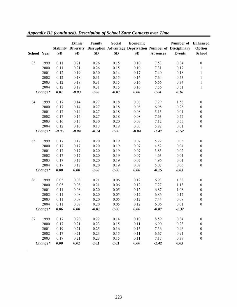
Appendix D2 (continued). Description of School Zone Contexts over Time

School YearStability

SD

Ethnic Diversity

SD

Family Disruption

SD

Social Advantage

SD

Economic Deprivation

SDNumber of Absences

Number of Disciplinary

Events

Enhanced Option School

52 1999 0.12 0.18 0.34 0.10 0.13 7.25 0.10 02000 0.12 0.18 0.34 0.10 0.13 8.06 0.11 02001 0.14 0.17 0.32 0.10 0.12 6.51 0.09 02002 0.14 0.17 0.32 0.10 0.12 7.42 0.17 02003 0.14 0.17 0.32 0.10 0.12 8.21 0.14 02004 0.16 0.17 0.15 0.10 0.04 6.64 0.04 0

Change* 0.04 0.00 -0.18 0.00 -0.09 -0.61 -0.06

53 1999 0.17 0.16 0.32 0.18 0.15 6.94 0.37 02000 0.17 0.16 0.32 0.18 0.15 6.94 0.21 02001 0.16 0.16 0.32 0.17 0.15 6.91 0.19 02002 0.17 0.16 0.31 0.17 0.15 7.28 0.13 02003 0.17 0.16 0.31 0.17 0.15 7.42 0.11 02004 0.19 0.14 0.17 0.16 0.09 7.93 0.13 0

Change* 0.02 -0.02 -0.16 -0.01 -0.07 0.99 -0.23

54 1999 0.12 0.15 0.22 0.07 0.08 10.43 0.99 02000 0.12 0.15 0.22 0.07 0.08 10.48 1.19 02001 0.12 0.14 0.22 0.07 0.07 11.69 2.41 0

Change* 0.00 -0.01 0.00 0.00 0.00 1.26 1.42

55 1999 0.15 0.20 0.22 0.21 0.13 8.77 0.13 02000 0.15 0.20 0.22 0.21 0.13 7.83 0.28 0

Change* 0.00 0.00 0.00 0.00 0.00 -0.94 0.15

56 2001 0.19 0.15 0.30 0.23 0.14 8.57 0.24 02002 0.19 0.15 0.31 0.23 0.14 9.48 0.38 02003 0.20 0.16 0.33 0.22 0.14 9.24 0.46 02004 0.20 0.16 0.33 0.23 0.14 10.26 0.24 0

Change* 0.00 0.01 0.03 0.00 0.01 1.69 0.00

57 1999 0.13 0.08 0.26 0.10 0.12 6.81 0.19 02000 0.13 0.08 0.26 0.10 0.12 6.55 0.22 02001 0.14 0.08 0.28 0.10 0.12 7.55 0.34 02002 0.14 0.08 0.28 0.10 0.12 6.70 0.10 02003 0.14 0.08 0.28 0.10 0.12 6.53 0.55 02004 0.14 0.08 0.28 0.10 0.12 5.93 0.24 0

Change* 0.01 0.00 0.01 0.00 0.00 -0.88 0.05

58 2001 0.10 0.15 0.22 0.07 0.12 5.05 0.92 02002 0.10 0.15 0.22 0.07 0.12 6.14 1.55 02003 0.10 0.15 0.22 0.07 0.12 7.02 0.58 02004 0.10 0.15 0.22 0.07 0.12 6.88 0.11 0

Change* 0.00 0.00 0.00 0.00 0.00 1.83 -0.81

218

Appendix D2 (continued). Description of School Zone Contexts over Time

School YearStability

SD

Ethnic Diversity

SD

Family Disruption

SD

Social Advantage

SD

Economic Deprivation

SDNumber of Absences

Number of Disciplinary

Events

Enhanced Option School

59 1999 0.11 0.17 0.32 0.21 0.14 6.88 0.43 02000 0.11 0.17 0.32 0.21 0.14 6.36 0.16 02001 0.11 0.17 0.32 0.21 0.14 6.09 0.34 02002 0.12 0.16 0.31 0.22 0.14 6.10 0.33 02003 0.12 0.16 0.31 0.22 0.14 5.86 0.17 02004 0.12 0.16 0.11 0.21 0.09 5.81 0.03 0

Change* 0.02 0.00 -0.20 0.00 -0.05 -1.07 -0.40

60 1999 0.12 0.19 0.27 0.09 0.08 6.02 0.44 02000 0.18 0.19 0.27 0.13 0.08 6.28 0.23 02001 0.14 0.15 0.24 0.07 0.06 6.51 0.13 02002 0.15 0.18 0.23 0.09 0.08 6.23 0.07 02003 0.15 0.18 0.23 0.09 0.08 7.09 0.06 02004 0.15 0.18 0.23 0.09 0.08 7.25 0.15 0

Change* 0.03 -0.01 -0.03 0.00 -0.01 1.22 -0.29

61 1999 0.12 0.19 0.28 0.08 0.11 10.02 3.65 02000 0.14 0.19 0.28 0.08 0.11 9.06 2.76 02001 0.17 0.18 0.26 0.10 0.10 8.56 2.59 02002 0.17 0.18 0.26 0.10 0.10 7.54 1.82 02003 0.15 0.18 0.26 0.08 0.10 8.71 1.92 02004 0.15 0.18 0.26 0.08 0.10 8.84 2.77 0

Change* 0.03 -0.01 -0.02 0.01 -0.01 -1.18 -0.88

62 1999 0.08 0.06 0.21 0.02 0.08 7.42 1.16 02000 0.08 0.06 0.21 0.02 0.08 7.19 1.02 02001 0.08 0.06 0.21 0.02 0.08 6.87 1.73 02002 0.08 0.06 0.21 0.02 0.08 7.57 0.27 02003 0.08 0.06 0.21 0.02 0.08 6.63 0.25 02004 0.08 0.06 0.21 0.02 0.08 6.38 0.19 0

Change* 0.00 0.00 0.00 0.00 0.00 -1.05 -0.97

63 2002 0.16 0.13 0.12 0.12 0.04 7.46 0.84 02003 0.16 0.13 0.12 0.12 0.04 8.39 0.27 02004 0.16 0.13 0.12 0.12 0.04 9.09 1.38 0

Change* 0.00 0.00 0.00 0.00 0.00 1.63 0.53

64 1999 0.14 0.19 0.26 0.08 0.08 7.02 0.31 02000 0.14 0.15 0.22 0.08 0.08 4.51 0.18 02001 0.14 0.15 0.22 0.08 0.08 4.25 0.17 0

Change* 0.00 -0.03 -0.03 0.00 0.00 -2.77 -0.15

219

Appendix D2 (continued). Description of School Zone Contexts over Time

School YearStability

SD

Ethnic Diversity

SD

Family Disruption

SD

Social Advantage

SD

Economic Deprivation

SDNumber of Absences

Number of Disciplinary

Events

Enhanced Option School

65 1999 0.11 0.10 0.36 0.12 0.18 7.05 0.10 02000 0.11 0.10 0.36 0.12 0.18 6.42 0.09 02001 0.11 0.10 0.36 0.12 0.18 6.91 0.12 02002 0.11 0.10 0.36 0.12 0.18 6.49 0.36 02003 0.11 0.10 0.36 0.12 0.18 6.80 0.07 02004 0.11 0.10 0.36 0.12 0.18 6.31 0.09 0

Change* 0.00 0.00 0.00 0.00 0.00 -0.74 -0.01

66 1999 0.14 0.14 0.27 0.09 0.12 13.72 2.08 02000 0.14 0.14 0.27 0.09 0.12 10.72 2.67 02001 0.14 0.15 0.26 0.09 0.12 9.55 2.24 02002 0.13 0.15 0.25 0.09 0.12 9.44 3.17 02003 0.12 0.14 0.21 0.07 0.10 8.92 2.73 02004 0.12 0.14 0.21 0.07 0.10 8.44 2.46 0

Change* -0.01 0.00 -0.06 -0.02 -0.02 -5.28 0.38

67 1999 0.15 0.13 0.33 0.16 0.17 11.42 0.49 02000 0.15 0.13 0.33 0.16 0.17 9.82 1.00 02001 0.15 0.13 0.33 0.16 0.17 9.02 0.72 02004 0.15 0.13 0.32 0.16 0.17 8.18 0.01 0

Change* 0.00 0.00 -0.01 0.00 0.00 -3.24 -0.47

68 1999 0.24 0.21 0.24 0.07 0.14 7.55 0.14 02000 0.23 0.16 0.24 0.07 0.14 5.01 0.16 02001 0.23 0.15 0.20 0.07 0.10 7.91 0.06 0

Change* 0.00 -0.06 -0.04 0.00 -0.05 0.36 -0.08

69 1999 0.18 0.20 0.37 0.18 0.16 6.71 0.21 02000 0.18 0.20 0.37 0.18 0.16 5.28 0.15 02001 0.19 0.19 0.39 0.18 0.17 7.63 0.38 02002 0.19 0.18 0.40 0.19 0.17 7.01 0.10 02003 0.17 0.17 0.34 0.16 0.13 7.70 0.37 02004 0.17 0.19 0.28 0.15 0.05 6.21 0.17 0

Change* -0.01 0.00 -0.09 -0.02 -0.11 -0.50 -0.04

70 1999 0.21 0.16 0.28 0.10 0.14 8.63 2.28 02000 0.21 0.16 0.28 0.10 0.14 9.21 2.79 02001 0.22 0.15 0.31 0.10 0.16 7.86 1.86 02002 0.22 0.15 0.31 0.10 0.16 8.39 1.67 02003 0.22 0.15 0.31 0.10 0.16 7.47 1.95 0

Change* 0.01 -0.01 0.03 0.00 0.01 -1.16 -0.33

220

Appendix D2 (continued). Description of School Zone Contexts over Time

School YearStability

SD

Ethnic Diversity

SD

Family Disruption

SD

Social Advantage

SD

Economic Deprivation

SDNumber of Absences

Number of Disciplinary

Events

Enhanced Option School

71 1999 0.16 0.19 0.24 0.17 0.10 8.13 0.36 02000 0.16 0.19 0.23 0.17 0.09 8.33 0.71 02001 0.17 0.19 0.24 0.17 0.10 7.29 0.52 02002 0.17 0.19 0.24 0.17 0.10 7.27 0.86 02003 0.18 0.20 0.23 0.16 0.09 6.56 1.98 02004 0.18 0.20 0.21 0.15 0.09 8.16 1.09 0

Change* 0.02 0.01 -0.03 -0.02 0.00 0.03 0.72

72 2002 0.15 0.16 0.13 0.08 0.05 5.35 0.03 02003 0.17 0.17 0.13 0.08 0.05 6.80 0.01 02004 0.17 0.17 0.13 0.08 0.05 6.11 0.00 0

Change* 0.01 0.02 0.00 0.01 0.00 0.76 -0.03

73 1999 0.11 0.15 0.23 0.08 0.11 5.91 0.17 02000 0.11 0.15 0.23 0.08 0.11 6.68 0.44 02001 0.12 0.15 0.21 0.08 0.09 5.50 0.34 02002 0.13 0.16 0.22 0.08 0.09 5.43 0.12 02003 0.13 0.16 0.22 0.08 0.09 6.54 0.20 02004 0.13 0.16 0.22 0.08 0.09 5.85 0.05 0

Change* 0.02 0.01 -0.01 0.00 -0.02 -0.06 -0.12

74 1999 0.20 0.17 0.24 0.20 0.12 8.29 0.38 02000 0.20 0.17 0.24 0.20 0.12 9.84 0.79 02001 0.20 0.17 0.23 0.20 0.12 9.04 0.61 02002 0.17 0.17 0.24 0.20 0.09 7.61 1.67 02003 0.16 0.17 0.22 0.20 0.08 8.10 1.26 02004 0.16 0.17 0.25 0.20 0.09 7.65 1.47 0

Change* -0.03 0.00 0.01 0.00 -0.03 -0.64 1.10

75 1999 0.06 0.14 0.08 0.07 0.04 5.23 0.09 02000 0.06 0.14 0.08 0.07 0.04 7.92 0.10 0

Change* 0.00 0.00 0.00 0.00 0.00 2.70 0.00

76 2000 0.13 0.18 0.13 0.16 0.05 4.65 0.05 02001 0.13 0.18 0.13 0.16 0.05 5.71 0.03 02002 0.13 0.18 0.13 0.16 0.05 5.57 0.03 02003 0.13 0.18 0.13 0.16 0.05 5.91 0.03 02004 0.13 0.18 0.13 0.16 0.05 5.60 0.07 0

Change* 0.00 0.00 0.00 0.00 0.00 0.95 0.02

221

Appendix D2 (continued). Description of School Zone Contexts over Time

School YearStability

SD

Ethnic Diversity

SD

Family Disruption

SD

Social Advantage

SD

Economic Deprivation

SDNumber of Absences

Number of Disciplinary

Events

Enhanced Option School

77 1999 0.18 0.18 0.18 0.12 0.08 9.59 0.86 02000 0.17 0.18 0.20 0.13 0.09 8.73 1.31 02001 0.17 0.17 0.19 0.13 0.09 8.78 0.70 02002 0.17 0.17 0.20 0.13 0.09 7.03 0.45 02003 0.16 0.17 0.23 0.16 0.10 8.52 2.00 02004 0.16 0.17 0.23 0.16 0.10 8.56 1.92 0

Change* -0.02 -0.01 0.05 0.03 0.02 -1.03 1.06

78 2001 0.08 0.20 0.18 0.05 0.11 3.81 1.71 12002 0.08 0.20 0.18 0.05 0.11 7.89 0.33 12003 0.08 0.20 0.18 0.05 0.11 6.75 0.31 12004 0.08 0.20 0.18 0.05 0.11 7.87 0.47 1

Change* 0.00 0.00 0.00 0.00 0.00 4.05 -1.24

79 1999 0.18 0.18 0.19 0.08 0.08 6.09 0.15 02000 0.18 0.18 0.19 0.08 0.08 6.04 0.11 02001 0.20 0.16 0.14 0.08 0.05 5.20 0.02 02002 0.20 0.16 0.14 0.08 0.05 6.35 0.08 02003 0.20 0.16 0.14 0.08 0.05 5.84 0.00 02004 0.20 0.16 0.14 0.08 0.05 6.10 0.00 0

Change* 0.02 -0.01 -0.05 0.01 -0.03 0.01 -0.15

80 1999 0.16 0.16 0.20 0.10 0.10 11.16 0.58 02000 0.16 0.16 0.20 0.10 0.10 10.87 1.41 02001 0.17 0.16 0.20 0.10 0.10 10.78 0.44 02002 0.18 0.15 0.18 0.10 0.10 10.22 2.61 02003 0.18 0.15 0.18 0.10 0.10 10.27 0.43 02004 0.18 0.15 0.18 0.10 0.10 10.71 0.85 0

Change* 0.01 -0.01 -0.02 0.00 0.00 -0.45 0.26

81 1999 0.15 0.17 0.20 0.11 0.05 5.98 0.03 02000 0.15 0.17 0.20 0.11 0.05 6.19 0.07 02001 0.14 0.16 0.25 0.12 0.06 5.86 0.28 02002 0.12 0.19 0.22 0.11 0.06 7.03 0.06 02003 0.12 0.19 0.22 0.11 0.06 7.60 0.01 02004 0.12 0.19 0.22 0.11 0.06 7.74 0.02 0

Change* -0.03 0.02 0.01 0.00 0.01 1.76 -0.01

82 1999 0.15 0.19 0.18 0.06 0.15 7.32 1.23 02000 0.15 0.19 0.18 0.06 0.15 7.35 1.51 02001 0.15 0.17 0.15 0.05 0.09 5.61 0.36 02002 0.15 0.17 0.15 0.05 0.09 5.35 0.12 02003 0.15 0.17 0.15 0.05 0.09 6.10 0.03 02004 0.15 0.17 0.15 0.05 0.09 5.81 0.03 0

Change* 0.01 -0.02 -0.03 -0.01 -0.06 -1.51 -1.20

222

Appendix D2 (continued). Description of School Zone Contexts over Time

School YearStability

SD

Ethnic Diversity

SD

Family Disruption

SD

Social Advantage

SD

Economic Deprivation

SDNumber of Absences

Number of Disciplinary

Events

Enhanced Option School

83 1999 0.11 0.21 0.26 0.15 0.10 7.53 0.34 02000 0.11 0.21 0.26 0.15 0.10 7.31 0.17 12001 0.12 0.19 0.30 0.14 0.17 7.40 0.18 12002 0.12 0.18 0.31 0.15 0.16 7.64 0.53 12003 0.12 0.18 0.31 0.15 0.16 6.66 0.34 12004 0.12 0.18 0.31 0.15 0.16 7.56 0.51 1

Change* 0.01 -0.03 0.06 -0.01 0.06 0.04 0.16

84 1999 0.17 0.14 0.27 0.18 0.08 7.29 1.58 02000 0.17 0.14 0.27 0.18 0.08 6.98 0.28 02001 0.17 0.14 0.27 0.18 0.08 5.15 0.01 02002 0.17 0.14 0.27 0.18 0.08 7.63 0.57 02003 0.16 0.15 0.30 0.20 0.09 7.12 0.55 02004 0.12 0.10 0.13 0.18 0.05 5.82 0.01 0

Change* -0.05 -0.04 -0.14 0.00 -0.04 -1.47 -1.57

85 1999 0.17 0.17 0.20 0.19 0.07 5.22 0.03 02000 0.17 0.17 0.20 0.19 0.07 4.52 0.04 02001 0.17 0.17 0.20 0.19 0.07 3.83 0.02 02002 0.17 0.17 0.20 0.19 0.07 4.63 0.01 02003 0.17 0.17 0.20 0.19 0.07 4.96 0.01 02004 0.17 0.17 0.20 0.19 0.07 5.07 0.06 0

Change* 0.00 0.00 0.00 0.00 0.00 -0.15 0.03

86 1999 0.05 0.08 0.21 0.06 0.12 6.93 1.38 02000 0.05 0.08 0.21 0.06 0.12 7.27 1.13 02001 0.11 0.08 0.20 0.05 0.12 6.87 1.08 02002 0.11 0.08 0.20 0.05 0.12 6.86 0.17 02003 0.11 0.08 0.20 0.05 0.12 7.44 0.08 02004 0.11 0.08 0.20 0.05 0.12 6.06 0.01 0

Change* 0.06 0.00 -0.01 0.00 0.00 -0.87 -1.37

87 1999 0.17 0.20 0.22 0.14 0.10 8.59 0.34 02000 0.17 0.21 0.23 0.15 0.11 6.90 0.23 02001 0.19 0.21 0.25 0.16 0.13 7.36 0.46 02002 0.17 0.21 0.23 0.15 0.11 6.67 0.91 02003 0.17 0.21 0.23 0.15 0.11 7.17 0.37 0

Change* 0.00 0.01 0.01 0.01 0.00 -1.42 0.03

223

Appendix D2 (continued). Description of School Zone Contexts over Time

School YearStability

SD

Ethnic Diversity

SD

Family Disruption

SD

Social Advantage

SD

Economic Deprivation

SDNumber of Absences

Number of Disciplinary

Events

Enhanced Option School

88 1999 0.15 0.12 0.32 0.17 0.12 5.45 0.20 02000 0.15 0.12 0.32 0.17 0.12 5.16 0.18 02001 0.15 0.12 0.32 0.17 0.12 4.26 0.30 02002 0.15 0.12 0.32 0.17 0.12 3.01 0.01 02003 0.15 0.12 0.32 0.17 0.12 5.16 0.23 02004 0.14 0.12 0.32 0.16 0.11 4.42 0.23 0

Change* -0.01 0.00 0.01 -0.01 -0.01 -1.03 0.03

89 1999 0.14 0.16 0.27 0.11 0.06 8.44 0.71 02000 0.14 0.16 0.27 0.11 0.06 6.55 0.10 02001 0.14 0.17 0.25 0.10 0.07 7.70 0.27 02002 0.14 0.17 0.25 0.10 0.07 6.74 0.49 02003 0.14 0.17 0.25 0.10 0.07 8.32 0.19 02004 0.14 0.17 0.25 0.10 0.07 7.18 0.15 0

Change* 0.00 0.00 -0.02 -0.01 0.01 -1.27 -0.56

90 1999 0.17 0.16 0.24 0.19 0.09 5.92 0.22 02000 0.17 0.16 0.24 0.19 0.09 5.93 0.12 02001 0.17 0.16 0.24 0.19 0.09 6.10 0.28 02002 0.17 0.16 0.25 0.20 0.10 5.49 0.02 0

Change* 0.00 0.00 0.01 0.00 0.00 -0.43 -0.20

91 1999 0.17 0.16 0.30 0.11 0.17 7.22 0.12 02000 0.17 0.16 0.30 0.11 0.17 8.22 0.07 02001 0.18 0.16 0.30 0.12 0.16 8.16 0.12 02002 0.17 0.15 0.29 0.11 0.15 9.36 0.06 02003 0.17 0.15 0.29 0.11 0.15 9.03 0.14 02004 0.16 0.14 0.19 0.11 0.11 7.02 0.07 0

Change* -0.01 -0.02 -0.11 0.00 -0.06 -0.20 -0.05

92 1999 0.12 0.14 0.33 0.24 0.15 6.99 0.02 02000 0.12 0.14 0.33 0.24 0.16 5.95 0.02 02001 0.12 0.15 0.33 0.23 0.16 6.25 0.04 02002 0.12 0.19 0.29 0.22 0.13 7.38 0.11 02003 0.12 0.19 0.26 0.21 0.12 7.72 0.08 02004 0.12 0.20 0.24 0.20 0.11 7.15 0.06 0

Change* 0.00 0.06 -0.08 -0.04 -0.05 0.16 0.04

93 1999 0.12 0.14 0.28 0.12 0.13 7.28 0.08 02000 0.12 0.14 0.28 0.12 0.13 8.01 0.19 02001 0.12 0.14 0.28 0.12 0.13 6.91 0.23 02002 0.12 0.14 0.28 0.12 0.13 5.99 0.05 02003 0.12 0.14 0.28 0.12 0.13 7.59 0.04 02004 0.13 0.13 0.12 0.11 0.07 6.67 0.03 0

Change* 0.01 -0.02 -0.15 -0.01 -0.06 -0.61 -0.05

224

Appendix D2 (continued). Description of School Zone Contexts over Time

School YearStability

SD

Ethnic Diversity

SD

Family Disruption

SD

Social Advantage

SD

Economic Deprivation

SDNumber of Absences

Number of Disciplinary

Events

Enhanced Option School

94 1999 0.15 0.17 0.22 0.09 0.11 6.23 0.09 02000 0.15 0.17 0.22 0.09 0.11 6.37 0.04 02001 0.15 0.17 0.22 0.09 0.11 5.96 0.03 02002 0.16 0.18 0.24 0.10 0.12 6.57 0.12 02003 0.16 0.22 0.13 0.11 0.06 7.02 0.05 02004 0.16 0.22 0.13 0.11 0.06 6.44 0.02 0

Change* 0.01 0.05 -0.09 0.02 -0.04 0.20 -0.07

95 1999 0.20 0.18 0.29 0.21 0.16 12.62 0.47 02000 0.20 0.18 0.29 0.20 0.16 10.28 1.16 02001 0.20 0.19 0.31 0.21 0.16 9.55 0.85 02002 0.19 0.17 0.33 0.21 0.15 9.25 0.83 02003 0.17 0.15 0.31 0.18 0.12 8.82 1.15 02004 0.19 0.18 0.21 0.20 0.09 8.01 0.66 0

Change* -0.01 0.00 -0.09 -0.01 -0.07 -4.60 0.19

96 1999 0.13 0.18 0.26 0.14 0.19 5.30 0.03 02000 0.13 0.17 0.26 0.14 0.19 5.70 0.02 02001 0.15 0.13 0.25 0.12 0.12 4.77 0.03 02002 0.15 0.12 0.25 0.12 0.12 5.07 0.03 02003 0.15 0.12 0.25 0.12 0.12 4.87 0.04 02004 0.15 0.12 0.25 0.12 0.12 5.65 0.00 0

Change* 0.02 -0.05 -0.02 -0.02 -0.07 0.35 -0.03

97 1999 0.14 0.14 0.27 0.08 0.05 6.35 0.23 02000 0.16 0.16 0.30 0.08 0.06 5.82 0.30 0

Change* 0.02 0.02 0.03 0.00 0.01 -0.54 0.08

98 2004 0.17 0.17 0.33 0.15 0.13 8.98 3.38 0Change* 0.00 0.00 0.00 0.00 0.00 0.00 0.00

99 1999 0.16 0.12 0.34 0.15 0.16 7.43 0.32 02000 0.16 0.12 0.34 0.15 0.16 6.99 0.26 02001 0.16 0.12 0.34 0.15 0.16 8.01 0.48 02002 0.16 0.12 0.34 0.15 0.16 6.81 0.37 02003 0.15 0.13 0.32 0.16 0.17 6.59 0.17 0

Change* -0.01 0.01 -0.03 0.01 0.01 -0.84 -0.16

100 1999 0.19 0.16 0.33 0.22 0.16 11.23 0.44 02000 0.19 0.16 0.33 0.22 0.16 12.39 0.88 02001 0.20 0.16 0.33 0.23 0.16 11.93 1.77 02002 0.20 0.18 0.28 0.23 0.16 6.49 1.05 02003 0.20 0.19 0.29 0.23 0.16 8.74 0.75 02004 0.18 0.19 0.32 0.23 0.17 8.61 1.35 0

Change* -0.02 0.03 -0.01 0.01 0.01 -2.62 0.92

225

r

Appendix D2 (continued). Description of School Zone Contexts over Time

School YearStability

SD

Ethnic Diversity

SD

Family Disruption

SD

Social Advantage

SD

Economic Deprivation

SDNumber of Absences

Number of Disciplinary

Events

Enhanced Option School

101 1999 0.17 0.17 0.29 0.19 0.12 6.28 0.04 02000 0.17 0.17 0.29 0.19 0.12 6.78 0.11 02001 0.17 0.17 0.29 0.19 0.12 6.41 0.13 02002 0.17 0.17 0.30 0.20 0.13 7.22 0.16 02003 0.17 0.17 0.30 0.20 0.13 7.70 0.12 02004 0.19 0.19 0.36 0.20 0.13 7.08 0.16 0

Change* 0.02 0.02 0.07 0.02 0.01 0.79 0.12

102 1999 0.21 0.19 0.27 0.17 0.15 14.13 2.31 02000 0.21 0.19 0.27 0.17 0.15 11.54 0.46 02001 0.21 0.19 0.27 0.17 0.15 11.13 1.98 02002 0.21 0.18 0.29 0.13 0.14 11.56 2.44 02003 0.20 0.18 0.29 0.13 0.14 13.52 1.50 02004 0.19 0.16 0.28 0.12 0.15 12.30 2.33 0

Change* -0.01 -0.03 0.01 -0.05 0.00 -1.82 0.02

103 1999 0.10 0.10 0.12 0.06 0.06 6.90 0.15 02000 0.10 0.10 0.12 0.06 0.06 6.99 0.09 02001 0.15 0.15 0.24 0.22 0.17 6.62 0.23 02002 0.14 0.15 0.27 0.21 0.16 6.40 0.05 02003 0.14 0.15 0.27 0.21 0.16 6.77 0.06 02004 0.14 0.15 0.27 0.21 0.16 5.83 0.03 0

Change* 0.04 0.06 0.15 0.15 0.11 -1.06 -0.12

104 1999 0.18 0.19 0.27 0.18 0.15 13.07 1.21 02000 0.18 0.19 0.27 0.18 0.15 11.60 2.41 02001 0.18 0.19 0.23 0.15 0.13 9.98 1.80 02002 0.17 0.19 0.23 0.14 0.12 8.47 1.11 02003 0.17 0.19 0.23 0.14 0.12 9.00 0.40 02004 0.17 0.19 0.23 0.14 0.12 9.40 0.59 0

Change* -0.01 0.00 -0.03 -0.04 -0.03 -3.67 -0.62

District 1999 0.157 0.163 0.257 0.134 0.118 7.66 0.655 ―

2000 0.157 0.163 0.253 0.134 0.116 7.319 0.572 ―2001 0.159 0.159 0.251 0.133 0.111 7.060 0.572 ―2002 0.155 0.160 0.245 0.135 0.108 7.045 0.559 ―2003 0.155 0.161 0.240 0.132 0.106 7.388 0.596 ―2004 0.153 0.160 0.232 0.131 0.102 7.200 0.606 ―

All Yea 0.156 0.161 0.246 0.133 0.111 7.277 0.593 ―

Avg. Change* -0.004 -0.003 -0.026 -0.004 -0.016 -0.460 -0.049 ―

*Change is calculated by subtracting values from 2004 from the baseline values for 1999. When a school was not opened in 1999 or 2004, values for the latest year were subtracted from values in the earliest year.

226

REFERENCES

Ainsworth, J. W. (2002). Why does it take a village? The mediation of neighborhood effects on educational achievement. Social Forces 81(1): 117-152.

Alexander, K. L., Entwisle, D. R., & Horsey, C. S. (1997). From first grade forward:

Early foundations of high school dropouts. Sociology of Education, 70: 87-107. Allan, G. (1996). Kinship and friendship in modern Britain. London: Oxford University

Press. Anderson, A. R., Christenson, S. L., Sinclair, M. F., & Lehr, C. A. (2004). Check &

connect: The importance of relationships for promoting engagement with school. Journal of School Psychology, 42(2): 95-113.

Baron, R. M. & Kenny, D. A. (1986). The moderator-mediator variable distinction in

social psychological research: Conceptual, strategic, and statistical considerations. Journal of Personality and Social Psychology, 51(6), 1173-1182.

Beem, C. (1999). The necessity of politics: Reclaiming American public life. Chicago:

University of Chicago Press. Bell, C. & Newby, H. (1972). Community studies. Westport, CT: Praeger. Bellair, P. E., (1997). Social interaction and community crime: Examining the importance

of neighbor networks. Criminology, 35: 677-701. Berry, J. M., Portney, K. E., & Thomson, K. (1991). The political behavior of poor

people. In C. Jencks & P. E. Peterson (Eds.), The urban underclass (pp. 357-372). Washongton, DC: The Brookings Institution.

Bott, E. (1957). Family and social networks. London: Tavistock. Brooks-Gunn, J., Duncan, G. J., Klebanov, P. K., & Sealand, N. (1993). Do

neighborhoods influence child and adolescent development? American Journal of Sociology, 99(2), 353-395.

Brown, R. B., Xu, X. Toth, J. F., & Nylander, A. B. (1998). Historical decline of

community satisfaction in U.S. rural communities: A multi-regional analysis of synthetic cohorts. Research in Community Sociology, 8,183-99.

Buber, M. (1947). Between man and man. Translated by R. G. Smith. London: Kegan

Paul. Bursik, J. R. (1988). Social disorganization and theories of crime and delinquency.

Criminology, 26, 519-551.

227

Bursik, R. J., Jr. & Grasmick, H. G. (1993). Neighborhoods and crime. New York:

Lexington Books. Burton, V. S. & Cullen, F. T. (1992). The empirical status of strain theory. Journal of

Crime & Justice 15:1-30. Catsambis, S. & Beveridge, A. A. (2001). Neighborhood and school influences on the

family life and mathematics performance of eighth-grade students. Washington, DC. (OERI No. R-117-D40005)

Cohen, A. (1955). Delinquent boys. New York: Free Press. Cohen, A. P. (1985). The Symbolic Construction of Community. London: Tavistock. Cohen, J., Cohen, P., West, S. G., & Aiken, L. S. (2003). Applied multiple

regression/correlation analysis for the behavioral sciences (3rd ed.). Mahwah, NJ: Lawrence Erlbaum Associates.

Coleman, J. S., Campbell, E. Q., Hobson, J. McPartland, J., Mood, A. M., Weinfeld, F.

D., & York, R. L. (1966). Equality of educational opportunity. Washington, DC: US Congressional Printing Office.

Comer, J. P. (1980). School power: Implications of an intervention project. London: Free

Press. Crane, J. (1991a). Effects of neighborhoods on dropping out of school and teenage

childbearing. In C. Jencks & P. E. Peterson (Eds.), The urban underclass (pp. 299-320). Washington, DC: The Brookings Institution.

Crane, J. (1991b). The epidemic theory of ghettos and neighborhood effects on dropping

out and teenage childbearing. American Journal of Sociology, 96(5), 1225-1259. Delado-Gaitan, C. (1992). School matters in the Mexican-American home. American

Educational Research Journal, 29, 495-513. Deutschberger, P. (1946). Interaction patterns in changing neighborhoods. Sociometry, 9,

303-315. Driscoll, M. E. (2001). The sense of place and the neighborhood school: Implications for

guiding social capital and for community development. In R. Crowson (Ed.), Community development and school reform, (pp. 19-42). New York: JAI Press.

228

Driscoll, M. E. & Kerchner, C. (1999). The implications of social capital for schools, communities and cities: Educational administration as if a sense of place mattered. In: J. Mirphy & K. Louis (Eds.), Handbook of Research on Educational Administration (2nd ed.) (pp. 385-404). San Francisco: Jossey Bass.

Durkheim, E. [1893] 1933. The division of labor in society. Translated by G.

Simpson. New York: Free Press. Egerton, J. (1996a). “The slow-burn years of Greensville school integration.” The

Tennessean. July 14.

Egerton, J. (1996b). “Busing brings integration conflict near boiling point. The Tennessean. January 21.

Egerton, J. (1996c). “Metro schools: Putting a finer finish on integration.” The Tennessean. January 28.

Elliott, D. S., Huizinga, D., & Ageton, S. S. (1985). Explaining delinquency and drug use. Beverly Hills, CA: Sage.

Elliott, D. S., Wilson, W. J., Huizinga, D., Sampson, R. J., Elliott, A., & Rankin, B.

(1996). The effects of neighborhood disadvantage and adolescent development. Journal of Research in Crime and Delinquency, 33: 389-426.

Erickson, K. T. (1976). Everything in its path: Destruction of community in the Buffalo

Creek Flood. New York: Touchstone Book.

Etzioni. A. (2000). Is bowling together sociologically lite? Contemporary Sociology, 30(3): 223-224.

Ferguson, R. (1998). Test score trends along racial lines, 1971 to 1996: Popular culture

and community academic standards. In National Research Council (Ed.), America becoming: Racial trends and their consequences: Vol. 1. (pp. 348-390). Washington, DC: National Academy Press.

Fischer, C. S. (1982). To dwell among friends. Chicago: University of Chicago Press.

Flinspack, S. L., Banks, K., & Khanna, R. (2003). Socioeconomic integration policy as a

tool for diversifying schools: Promise and practice in two large school systems. Paper presented at the Harvard Color Lines Conference, Cambridge.

Frankenberg, E. & Lee, C. (2002). Race in American public schools: Rapidly

resegregating school districts. Cambridge, MA: The Civil Rights Project, Harvard University.

229

Frankenberg, E., Lee, C., & Orfield, G. (2003). A multiracial society with segregated schools: Are we losing the dream? Cambridge, MA: The Civil Rights Project, Harvard University.

Frazer, E. (1999). The problem of communitarian politics: Unity and conflict. Oxford:

Oxford University Press. Freudenberg, W. R. (1986). The density of acquaintanceship: A overlooked variable in

community research? American Journal of Sociology 92, 27–63. Furstenberg, F. F., Jr., Cook, T. D., Eccles, J., Elder, G. H., Jr., & Sameroff, A. (1999).

Managing to make it: Urban families and adolescent success. Chicago: University of Chicago Press.

Gamoran, A., An, B., & Smrekar, C. E. (2005, April). Student achievement, racial

isolation, and the concentration of poverty. Paper presented at the Annual Meeting of the American Educational Research Association, Montreal.

Garner, C. L. & Raudenbush, S. W. (1991). Neighborhood effects on educational

attainment: A multilevel analysis. Sociology of Education, 64(4), 251-262. Gardner, W., Mulvey, E. P., & Shaw, E. C. (1995). Regression analyses of counts and

rates: Poisson, overdispersed Poisson, and negative binomial models. Psychological Bulletin, 118(3), 392-404.

Goldring, E., Cohen-Vogel, L., & Smrekar, C. (Under Review Teachers College Record,

2004). Neighborhood capacity in the ear of unitary status: What does “closer to home” really mean?

Goldring, E. & Crowson, R. (April, 2002). Unmaking desegregation policy and “going

unitary”: The loss of a sense of place. Paper presented at the annual meeting of the American Educational Research Association, New Orleans.

Goldring, E. B. & Rowley, K. J. (2005). Educational services for all: Academic opportunities and unitary status. Paper presented at the Annual Meeting of the American Educational Research Association; Montreal, Canada.

Goldring, E. B. & Smrekar C. (2002). Shifting from court-ordered to court-ended

desegregation in Greensville: Student assignment and teacher resources. Paper presented at The Resegregation of Southern Schools. A Crucial Moment in the History and Future of Public Schooling in America, August 2001, Chapel Hill, North Carolina.

Gruenewald, D. A. (2003). Foundations of place: A multidisciplinary framework for place-conscious education. American Educational Research Journal, 40(3), 619-654.

230

Gussow, A. (1971). A sense of place: The artist and the American landscape. San

Francisco: Friends of the Earth. Harrison, M. F. (Ed.). (1998). Summary of pupil assignment plan: Adopted by the

Greensville Metropolitan Public Schools—County, June 23, 1998). Willis & Knight.

Harvard Business School. (N.d.). “Building community.” Retrieved July 25, 2002 from

the World Wide Web: http://www.hbs.edu/it/main/initiatives_building.htm Harvey, D. (2001). Spaces of capital: Towards a critical geography. New York:

Routledge. Hirschi, T. (1969). Causes of delinquency. Berkeley, CA: University of California Press. Hogan, D. P. & Kitigawa, E. M. (1985). The impact of social status, family structure, and

neighborhood on the fertility of black adolescents. American Journal of Sociology, 90, 825-855.

Howell, D. (2002). Statistical methods for psychology (5th ed.). Belmont: Duxbury. Hummon, D. M. (1990). Commonplaces: Community ideology and identity in American

culture. Albany, New York: State University of New York Press. Irvine, R., & Irvine, J. (1984). The impact of the desegregation process on the education

of Black students: Key variables. Journal of Negro Education, 52, 410-422. Jones, F. (1981). A traditional model of educational excellence. Washington, DC:

Howard University Press. Kersten, K. (1995). Good intentions are not enough: The peril posed by Minnesota’s new

Desegregation plan. Minneapolis: Center for American Experiment. www.amexp.org/publications.

Kornhauser, R. R. (1978). Social sources of delinquency. Chicago: The University of

Chicago Press. Lamdin, D. J. (1996). Evidence of student attendance as an independent variable in

education production functions. Journal of Educational Research, 89: 155-162. Leach, W. (1999). Country of exiles: The destruction of place in American life. New

York: Pantheon.

231

Lewis, P. (1979). Defining a sense of place. In P. W. Prenshaw & J. O. McKee (Eds.), Sense of place: Mississippi, (pp. 24-46). Jackson, MS: University Press of Mississippi.

Liska, A. (1971). Aspirations and expectations. Sociological Quarterly 12: 99-107. Long, D. (2002, March 6). Bellshire: Centers suit unique needs. The Tennessean, pp. 1A,

2A. Massey, D. S. & Denton, N. (1993). American apartheid: Segregation and the making of

the underclass. Cambridge, MA: Harvard University Press. Mayer, S. E. (1991). How much does a high schools’ racial and socioeconomic mix affect

graduation and teenage fertility rates? In C. Jencks & P. E. Peterson (Eds.), The urban underclass (pp. 321-341). Washington, DC: The Brookings Institute.

Mayer, S. E. & Jencks, C. (1989). Growing up in poor neighborhoods: How much does it

matter? Science, 243(4897), 1441-1445. McKenzie, R. D. (1921). The neighborhood. In A. H. Hawley & R. D. McKenzie (Eds.),

On human ecology, (pp. 51-93). Chicago: University of Chicago Press. Metropolitan Board of Public Education of Greensville. (1993, December 16). School

Board Minutes. Greensville, TN. Metropolitan Board of Public Education of Greensville. (1994, October 4). School Board

Minutes. Greensville, TN. Metropolitan Board of Public Education of Greensville. (1995, April 25). School Board

Minutes. Greensville, TN. Metropolitan Board of Public Education of Greensville. (1997, June 10). School Board

Minutes. Greensville, TN. Metropolitan Board of Public Education of Greensville. (1997, September 9). School Board

Minutes. Greensville, TN. Metropolitan Board of Public Education of Greensville. (1998, January 23). School Board

Minutes. Greensville, TN. Metropolitan Board of Public Education of Greensville. (1998, June 23). School Board

Minutes. Greensville, TN.

232

Greensville Metropolitan Public Schools. (n.d.). Enhanced option schools. Greensville, TN.

Mickelson, R. A. (2001). Subverting Swann: First- and second-generation segregation in

Charlotte-Mecklenberg Schools. American Educational Research Journal, 38(2): 215-252.

Morenoff, J. D., & Tienda, M. (1997). Underclass neighborhoods in temporal and

ecological perspective. Annals of the American Academy of Political and Social Science Research, 20: 397-420.

Morris, J. (2001). Forgotten voice of Black educators: Critical race perspectives on the

implementation of a desegregation plan. Educational Policy, 15(4), 575-600. Morris, J. (1999). A pillar of strength: An African American school’s communal bonds’

with families and community since Brown. Urban Education, 33(5), 584-605. Myers, D. E., Milne, A. M., Baker, K., & Ginsburg, A. (1987). Student discipline and

high school performance. Sociology of Education, 60(1), 18-33. Nichols, J. D. (2004). An exploration of discipline and suspension data. Journal of Negro

Education, 73(4): 408-423. Orfield, G. (2003, November). Progress to retreat in school desegregation? Lecture

presented at Vanderbilt University, Greensville, TN. Orfield, G. (2001). Schools more separate: Consequences of a decade of resegregation.

Cambridge, MA: The Civil Rights Project, Harvard University. Orfield, G. (1999, June). Harvard Civil Rights Project. Retrieved October 4, 2003 from

the World Wide Web: http://www.law.harvard.edu/groups/civilrights/publications/resegregation 99.html

Orfield, G. & Eaton, S. E. (Eds.). (1996). Dismantling desegregation: The quiet reversal

of Brown v. Board of Education. New York: The New Press. Orfield, G. & Lee, C. (2004). Brown at 50: King’s dream or Plessy’s nightmare?

Cambridge, MA: The Civil Rights Project, Harvard University. Parcel, T. L. & Dufur, M. J. (2001). Capital at home and at school: Effects on student

achievement. Social Forces, 79(3), 881-912. Park, R. (1916). The city: Suggestions for the investigations of human behavior in the

urban environment. American Journal of Sociology, 20, 577-612. Park, R. & Burgess, E. W. (1925). The city. Chicago: University of Chicago Press.

233

Pelly-Effrat, M. (1974). Approaches to community: Conflicts and complimentarities. In

M. Pelly-Effrat (Ed.), The community (pp. 1-32). New York: The Free Press. Portes, A. (1998). Social Capital: Its origins and applications in modern sociology,

Annual Reviews, 24, 1-24. Pride, R. & May, H. V. M., Jr. (1999). Neighborhood schools again? Race, educational

interest, and traditional values, Urban Education, 34(3), 389-410. Putnam, R. D. (2000). Bowling alone: The collapse and revival of American community.

New York: Simon & Schuster. Raudenbush, S. W. & Bryk, A. S. (2002). Hierarchical linear models: Application and

data analysis methods (2nd ed.). Thousand Oaks, CA: Sage. Rheingold, H. (1993). The virtual community: Homesteading on the electronic frontier,

revised edition. Cambridge: MIT Press. Rumberger, R. W. (1995). Dropping out of middle school: A multilevel analysis of

students and schools. American Educational Research Journal, 23(3): 583-625. Rutman, D. B., & Rutman, A. H. (1984). A place in time: Middlesex County, Virginia,

1650–1750. New York: W. W. Norton. Ryan, B. A., Adams, G. R., Gullota, T. P., Weissberg, R. P, & Hampton, R. L. (1995).

The family-school connection: Theory, research, and practice. Thousand Oaks, CA: Sage.

Sampson, R. J. (1983). Structural density and criminal victimization. Criminology 21(2):

276-293. Sampson, R. J. (2000). The neighborhood context of investing in children: Racilitating

mechanisms and undermining risks. In S. Danzinger & J. Waldfogel (Eds.), Securing the future. New York: Russell Sage Foundation.

Sampson, R. J. & Groves, W. B. (1989). Neighborhood and delinquency: An assessment

of contextual effects. Criminology, 24, 667-699. Sampson, R. J., Morenoff, J. D., & Gannon-Rowley, T. (2002). Assessing “neighborhood

effects”: Social processes and new directions in research. Annual Review of Sociology, 28, 443-478.

Sampson, R. J. & Raudenbush, S. W. (1999). Systematic social observation of public

spaces: A new look at disorder in urban neighborhoods. American Journal of Sociology, 105(3), 603-651.

234

Schneider, B., & Coleman, J. S. (1993). Parents, their children, and schools. Boulder,

CO: Westview Press. Shaw, C. R. (1952). Brothers in crime. Chicago: University of Chicago Press. Shaw, C. R. & McKay, H. D. (1942). Juvenile delinquency and urban areas. Chicago:

University of Chicago Press. Shaw, C. R. & McKay, H. D. (1969). Juvenile delinquency and urban areas. A study of

rates of delinquency in relation to differential characteristics of local communities in American cities. Chicago: University of Chicago Press.

Shoemaker, D. (1996). Theories of delinquency: An examination of explanations of

delinquent behavior. 3rd ed. New York: Oxford University Press. Siddle-Walker, E. V. (1993). Caswell county training school, 1933-1969: Relationships

between community and school. Harvard Educational Review, 63(2), 161-182. Siddle-Walker, E. V. (1996). Their highest potential: An African American school

community in the segregated south. Chapel Hill: The University of North Carolina Press.

Simmel, G. [1903] (1983). “The metropolis and mental life.” In R. L. Warren and L.

Lyon (Eds.), New Perspectives on the American Community (pp. 18-27). Homewood, IL: Dorsey Press.

Singer, J. D. & Willett, J. B. (2003). Applied longitudinal data analysis: Modeling

change and event occurrence. New York: Oxford University Press. Suttles, G. D. (1972). The social construction of communities. Chicago: University of

Chicago Press. Taylor, R. B. (1996). Neighborhood responses to disorder and local attachments: The

systemic model of attachment, social disorganization, and neighborhood use value. Sociological Forum, 11(1), 41-74.

Toennies, F. [1935] (1983). “Gemeinschaft and gesellschaft.” In R. L. Warren and L.

Lyon (Eds.), New Perspectives on the American Community (pp. 7-16). Homewood, IL: Dorsey Press.

Trueba, H. T. (1988). Culturally based explanations of minority students’ academic

achievement. Anthropology and Education Quarterly, 19, 270-287.

235

University of Wisconsin-Milwaukee Employment and Training Institute. (2002). Racial integration in urban America: A block level analysis of African and White housing patterns. http://www.uwm.edu/Dept/ETI/integration/integration.pdf

US Census Bureau. (2000). Census 2000: Geographic terms and concepts.

http://www.census.gov/geo/www/tiger/glossry2.pdf US Department of Justice. (2002, April 24). Educational Opportunities Section:

Overview. Retrieved October 4, 2003 from the World Wide Web: http://www.usdoj.gov/crt/edo/overview.htm

Warner, B. D., & Rountree, P. W. (1997). Local social ties in a community and crime

model: Questioning the systemic nature of informal social control. Social Problems, 44: 520-536.

Warren, R. (1963). The community in America. Chicago: Rand McNally. Wells, S. E. (1990). At-risk youth: Identification programs, and recommendations.

Englewood, CO: Teacher Idea Press. Wenger, G. C. (1984). The supportive network. London: Allen & Unwin. Wenger, G. C. (1995). A comparison of urban and rural support networks. Ageing and

Society, 15: 59-81. Willie, C. V. (1990). Diversity, school improvement and choice. Education and Urban

Society, 23, 73-79. Willie, C. V., Alves, M., & Hagerty, C. (1996). Multiracial, attractive city schools:

Controlled choice in Boston. Equity and Excellence in Education, 29(2), 5-19. Willie, C. V., Alves, M., & Mitchell, C. (1998). Equity and excellence: A plan for

educational improvement of the Charleston County public schools. Charleston, SC: Charleston Planning Project for Public Education.

Wilson, W. J. (1987). The truly disadvantages: The inner city, the underclass, and public

policy. Chicago: University of Chicago Press. Wilson, W. J. (1996). When work disappears: The world of the new urban poor. Knopf. Wilson, W. J. (1998). The role of the environment in the Black-White test score gap. In

C. Jencks & M. Phillips (Eds.), The Black-White test score gap. Washington, DC: Brookings Institution Press.

236