Lead Time Estimation Using Artificial Intelligence

CONTACT William G. Dinnison Director, Defense Agencies +1.571.633.7853 office [email protected] LMI | 7940 Jones Branch Drive, Tysons, VA 22102

About Us LMI is a consultancy dedicated to improving the business of government, drawing from deep expertise in advanced analytics, digital services, logistics, and management advisory services. Established as a private, not-for-profit organization in 1961, LMI is a trusted third party to federal civilian and defense agencies, free of commercial and political bias.

Learn more at lmi.org

Lead Time Estimation Using Artificial Intelligence

© 2020 LMI. All rights reserved. 11509.000.00L1

June 2020

ee

June 2020


Stephanie D. Brown

Hasan Khan

Russell S. Salley

Wei Zhu

NOTICE:

THE VIEWS, OPINIONS, AND FINDINGS CONTAINED IN THIS REPORT ARE THOSE OF LMI AND SHOULD NOT BE CONSTRUED AS AN OFFICIAL AGENCY POSITION, POLICY, OR DECISION, UNLESS SO DESIGNATED BY OTHER OFFICIAL DOCUMENTATION.

LMI ©2020. ALL RIGHTS RESERVED. 11509.000.00L1

iii

Lead Time Estimation Using Artificial Intelligence June 2020

Executive Summary

The Defense Logistics Agency (DLA) relies on accurate estimates of lead time—and its components of administrative lead time (ALT) and production lead time (PLT)—to decide what to buy, how much to buy, and when to buy. Those estimates influence operational efficiency and effectiveness; when they are wrong, warfighter readiness suffers.

The accuracy of ALT and PLT estimates affects inventory costs, backorder rates, and the efficient use of DLA obligation authority. If DLA overestimates lead times, it places orders too early and overstocks occur. Underestimated lead times create backorders and diminish mission readiness. Often, estimates rely on historical data for items with infrequent orders, not accounting for additional data sources that may improve accuracy.

DLA asked LMI to identify artificial intelligence (AI) methods that improve accuracy of total lead time (TLT) estimation and its component parts. AI methods can improve the accuracy of lead time estimates for ALT, PLT, and TLT by 19 to 40 percent. On average, random forest (RF) models improve the accuracy of lead time predictions by 38 days.

Summary of Technical Results DLA uses mean absolute error (MAE), the average absolute error across observations, to compare AI models to baseline methods. The administrative lead time of record (ALTR), production lead time of record (PLTR), and the one-third rule are baseline methods to forecast ALT and PLT. RF AI models are the most accurate for predicting ALT and PLT. When compared to the baseline one-third rule method, the RF models reduce the MAE by 32 percent (17 days) for ALT and 19 percent (16 days) for PLT (see Table ES-1).

Table ES-1. Overall ALT and PLT Model Scores

ALT model scores PLT model scores

Model MAE (days) Model MAE (days)

RF 37 RF 67 ALT one-third rule 53 PLT one-third rule 83 ALTR 56 PLTR 94

iv

AI methods incorporate a range of data and improve predictions for items with little or no lead time history. ALT and PLT RF models offer the largest improvements for infrequently procured items (see Figure ES-1 and Figure ES-2).

Figure ES-1. ALT MAE by Procurement Frequency

Figure ES-2. PLT MAE by Procurement Frequency

0

10

20

30

40

50

60

70

80

90

One-timebuy

Rare Every 2years

Annually Twice ayear

Quarterly Monthly

MAE

(day

s)

Procurement frequency

ALTR One-third rule RF

0

20

40

60

80

100

120

140

One-timebuy

Rare Every 2years


Quarterly Monthly

MAE

(day

s)


PLTR One-third rule RF

Executive Summary

v

For estimating TLT, we tested two approaches: building a third AI model to predict TLT and adding the outputs from the separate ALT and PLT AI models. Adding the predictions from the ALT and PLT RF models offers the greatest accuracy, reducing MAE by 40 percent (38 days) compared to the sum of the one-third rule baselines (see Table ES-2).

Table ES-2. TLT Model Scores

Model MAE (days)

ALT RF + PLT RF 56 ALT one-third + PLT one-third 94 ALTR + PLTR 111

The average of errors for TLT predictions is even across procurement frequency. This reduces the risks associated with inaccurate lead time estimates for infrequently procured items (see Figure ES-3).

Figure ES-3. TLT MAE by Procurement Frequency

Note: TLTR is the baseline total lead time of record.

Demonstrated Process Improvements The results of this research and development project show that by using the RF models DLA can improve total lead time MAE 40 percent. This provides the following improvements to DLA planning:

• Obligation Authority: RF models reduces requirements by $11 million annually for the subset of items analyzed. If this sample is representative, the results scale to a $102 million annual reduction in requirements for the entire item population.

0

20

40

60

80

100

120

140

160

One-timebuy

Rare Every 2years


Quarterly Monthly

MAE

(day

s)


TLTR One-third rule ALT RF + PLT RF

vi

• Inventory Storage: RF models save approximately $26 million in holding cost by reducing overestimated lead times. This does not include safety stock.

• Sudden Changes in Lead Times: RF models decrease the number of lead times flagged for manual review, reducing workload by 46 percent over the current method, which is in line with the total number of lead times that current forecast methods would flag without overrides or freezes.

• Backorders: Units backordered due to underestimated lead times decreases for Next Gen items and increases for Acquisition Advice Code (AAC) D and Non-Peak Policy and Next Generation™ AAC Z items. If the analysis sample is representative of the full item population, the results scale to a 7 percent increase. This increase can be offset by transferring inventory reductions to safety stock.

Although the RF models improve accuracy and supply better support for all procurement frequency buckets, the largest improvements are for the infrequently procured, hardest to predict items. From this research, we conclude that RF AI models should be used to estimate lead times with the initial focus on infrequently procured items.

Transition Recommendations Separate near-term and long-term transition plans are required. Additional funding of $412,000 is required to implement the near-term plan, where LMI will manage the AI models and update forecasts. This follow-on transition project should include additional analysis and model refinements to ensure a smooth transition. In the long term, LMI will work with J6 to approve the use of Python in DLA systems and integrate the AI models into the DLA systems.

vii

Contents

Introduction ...............................................................................................1-1

Background ............................................................................................................1-1

Objectives ...............................................................................................................1-2

Technical Approach ..................................................................................2-1

Data Collection .......................................................................................................2-2

DLA Data ..........................................................................................................2-2

External Data ....................................................................................................2-3

Data Processing and Cleansing ..............................................................................2-4

Feature Engineering ...............................................................................................2-6

Historical Aggregations of Features ..................................................................2-6

Date-Derived Features ......................................................................................2-7

Novel Features .................................................................................................2-7

Feature Engineering by Estimation Task ...........................................................2-8

Encoding and Scaling .............................................................................................2-8

Model Training ........................................................................................................2-9

Train Test Split—ALT and PLT ....................................................................... 2-10

Train Test Split—TLT ...................................................................................... 2-10

Training ........................................................................................................... 2-11

Model Evaluation .................................................................................................. 2-12

Baseline Forecasting Methods ........................................................................ 2-12

Evaluation Metrics ........................................................................................... 2-13

Analysis and Results ................................................................................3-1

ALT and PLT Predictive Models..............................................................................3-1

Overall Results .................................................................................................3-1

Procurement Frequency Breakdown .................................................................3-2

Direction of Error ...............................................................................................3-6

Feature Insight ..................................................................................................3-7

TLT Predictive Models .......................................................................................... 3-12

Overall Results ............................................................................................... 3-12

viii

Procurement Frequency Breakdown ............................................................... 3-13

Direction of Error ............................................................................................. 3-14

Risk Metric ............................................................................................................ 3-15

Business Benefits .....................................................................................4-1

Obligation Authority ................................................................................................4-2

Inventory Storage ...................................................................................................4-2

Sudden Changes in Lead Time...............................................................................4-3

Backorders .............................................................................................................4-4

Conclusions and Recommendations .......................................................5-1

Conclusions ............................................................................................................5-1

Recommendations ..................................................................................................5-2

Transition Planning ...................................................................................6-1

Appendix A Hardware and Software

Appendix B Feature Lists

Appendix C Aggregation Rules

Appendix D Model Parameters, Scores, and Significance

Appendix E ML Regression Model Descriptions

Appendix F Model Metrics

Appendix G Shifting Over- and Underestimate Distributions

Appendix H Magnitude and Direction of Error by Procurement Frequency

Appendix I Abbreviations

Figures Figure 2-1. Timeline of PR and Prediction ..............................................................2-1

Figure 2-2. Technical Approach ..............................................................................2-2

Figure 2-3. Masking Example .................................................................................2-3

Figure 2-4. Data Processing and Cleansing ............................................................2-4

Figure 2-5. Example of Procurement-Level Data Aggregations...............................2-6

Figure 2-6. Example of Historical Aggregation Engineered Feature ........................2-7

Figure 2-7. Profit Center Workload .........................................................................2-8

Figure 2-8. One-Hot Encoding Example .................................................................2-9

Figure 2-9. Model Training (ALT Example) .............................................................2-9

Figure 2-10. Using an AI Model to Predict (ALT Example) .................................... 2-10

Figure 2-11. TLT Holdout Set ............................................................................... 2-11

Contents

ix

Figure 2-12. Time Series Cross-Validation ........................................................... 2-12

Figure 3-1. ALT Test Set Procurement Frequency Distribution ...............................3-2

Figure 3-2. ALT MAE by Procurement Frequency...................................................3-3

Figure 3-3. ALT MAPE by Procurement Frequency ................................................3-4

Figure 3-4. PLT MAE by Procurement Frequency...................................................3-5

Figure 3-5. PLT MAPE by Procurement Frequency ................................................3-5

Figure 3-6. ALT Magnitude and Direction of Errors .................................................3-6

Figure 3-7. PLT Magnitude and Direction of Error ...................................................3-7

Figure 3-8. ALT DT Top 10 Important Features ......................................................3-9

Figure 3-9. ALT RF Top 10 Important Features ......................................................3-9

Figure 3-10. ALT LR Top 10 Impactful Features ................................................... 3-10

Figure 3-11. PLT DT Top 10 Important Features .................................................. 3-11

Figure 3-12. PLT RF Top 10 Important Features .................................................. 3-11

Figure 3-13. PLT LR Top 10 Impactful Features ................................................... 3-12

Figure 3-14. TLT MAE by Procurement Frequency ............................................... 3-13

Figure 3-15. TLT MAPE by Procurement Frequency ............................................ 3-14

Figure 3-16. TLT Magnitude and Direction of Error ............................................... 3-15

Figure 3-17. Predicted ALT (RF) with Mean Error Bars ......................................... 3-16

Figure 4-1. Item Population .....................................................................................4-1

Tables Table 2-1. TLT Estimation Methods ........................................................................2-1

Table 2-2. DLA Data Sources .................................................................................2-2

Table 2-3. External Data Table ...............................................................................2-4

Table 2-4. ML Model Tradeoffs ............................................................................. 2-12

Table 3-1. Overall ALT and PLT Model Scores .......................................................3-1

Table 3-2. Overall TLT Model Scores ................................................................... 3-12

Table 4-1. Requirements Reduction .......................................................................4-2

Table 4-2. Holding Cost Due to Overestimated Lead Times ...................................4-3

Table 4-3. Number of Lead Time Updates Flagged for Review ...............................4-4

Table 4-4. Expected Units Backordered Due to Underestimated Lead Times .........4-4

1-1

Introduction

The Defense Logistics Agency (DLA) relies on accurate estimates of lead time—and its components of administrative lead time (ALT) and production lead time (PLT)—to decide what to buy, how much to buy, and when to buy. Those estimates influence operational efficiency and effectiveness; when they are wrong, warfighter readiness suffers.

Background DLA’s ALT and PLT estimates rely on historical data for items with infrequent orders, not accounting for additional data sources that may improve accuracy. Estimation methods do not differentiate between types of items, types of contracts, or demand volume. The accuracy of ALT and PLT estimates affects inventory costs, backorder rates, and the efficient use of DLA obligation authority. If DLA overestimates lead times, it places orders too early and overstocks occur. Underestimated lead times create backorders and diminish mission readiness.

Current estimation methods work well for items that are procured frequently; however, a large portion of DLA’s catalog is procured infrequently, limiting available observations and consistent accuracy in predictions. These methods also fail to account for several significant data elements, process factors, and environmental influences on lead time. For example, a solicitation with an order quantity of 2 may have a significantly longer lead time than a procurement of 200 since few vendors maintain production lines for low-demand parts, necessitating a long set-up time to manufacture the part. Accuracy of lead time estimates is challenging when not accounting for these external data fields.

By expanding the dataset (to include DLA data not used for lead time predictions as well as other external sources) to produce predictions for an item from trends across all items and in groups of sufficiently similar items, artificial intelligence (AI) methods hold promise for overcoming the challenges of estimation methods. AI methods detect and uncover similarities and patterns between items, assessing common characteristics and procurement histories. AI models dynamically group items for estimation purposes. In prior LMI research for DLA,0F

1 we applied machine learning (ML) for better estimating PLT. The results translated to projected annual savings of approximately $23 million.

1 Michael D. Bosack et al., Production Lead Time Estimation, DL304T4 (Tysons, VA: LMI, July 2016).

1-2

Objectives The objectives for this research project are the following:

• Find, develop, and validate AI methods that improve accuracy of total lead time (TLT) estimation and its component parts: ALT and PLT.

• Derive a risk metric that describes variability in lead time estimates.

• Recommend ways to implement research, technical documentation, all developed code, and documented insights of challenges.

2-1

Technical Approach

Our technical approach consists of three parallel lines of analysis for ALT, PLT, and TLT estimation tasks. For each line of analysis, we built an ML model to replace DLA’s method of predicting the specific lead time component (ALT, PLT, or TLT). Each model offers a lead time prediction for each National Item Identification Number (NIIN) using only the data available at the time the prediction is made (i.e., time of inference). Since historical data trains and tests the ML models, special care is needed to ensure that only the data available at the time of inference is used.

The models apply purchase request (PR) and purchase order (PO) data. In ALT modeling, each PR record has an opened date (i.e., procurement date) and an award date (i.e., document date). The model predicts ALT on the PR opened date. The true value of ALT is observed on the day of PR award (see Figure 2-1). Each PR is transformed into a modeling record with features known only on the PR opened date. Data known at the time of inference include item attributes (e.g., supply chain and profit center) and information from past PRs awarded before this date. At the time of ALT prediction, information from the PR (e.g., document type and order quantity) are not yet known and cannot be included in this record. The same follows for PLT modeling, where the prediction is made on the PO award date and the true value is observed on the PO delivery date, and TLT modeling, where the prediction occurs on the PR opened date and the true value is observed on the PO delivery date.

Figure 2-1. Timeline of PR and Prediction

ALT and PLT are each predicted by building one distinct model, applying relevant features for each estimation task. In contrast, TLT is predicted using two modeling methods: the unified method, building and training a distinct TLT model over relevant features, and the composite method, summing lead time predictions from separate ALT models and PLT models to predict TLT. The target variable for both approaches is TLT (the sum of observed ALT and observed PLT). Table 2-1 describes the pros and cons.

Table 2-1. TLT Estimation Methods

Method Pros Cons

Unified Trained on TLT data, exactly matching the phenomenon predicted.

Less data is available to train models because PR and PO data is required.

Composite More data is available to train the individual ALT and PLT models.

Errors from individual ALT and PLT models may compound.

Time

Observed ALT

PR award datePR opened date

2-2

Each line of analysis followed the five-step process detailed in this chapter. The corresponding Jupyter notebook file structure for this process is outlined in Figure 2-2. See Appendix A for a complete technical data roadmap.

Figure 2-2. Technical Approach

Data Collection We built the lead time estimation models with data from multiple sources. DLA supplied data on past procurements and item characteristics. External data sources tested whether incorporating various market indicators could improve lead time estimates.

DLA Data DLA furnished much of the data in eight tables from the Enterprise Data Warehouse (EDW) and DLA Operations Research and Resource Analysis (DORRA) systems. DLA applied several filters and data cleansing steps before sending the final dataset to LMI (see Table 2-2).

Table 2-2. DLA Data Sources

Table description Source table Source system

Purchase Order Item Data CV_PR_BPURHO02 EDW Purchase Requisition/Solicitation Line Item Data

CV_PR_BPURHO05 EDW

Alternate Purchase Requisition (ZDOR_APR Interface Data) (Active Purchase Requisitions)

CV_PR_BPRWHO02 EDW

Item Detail CV_CS_ITEM_DETAIL EDW Material Master DORRADW_MATL_MASTER_DIMENSION DORRA Material Master (Historical) DORRADW_MTRL_MSTR_HIST_DIM DORRA Tech Quality CV_TQ_MATERIAL_CLASS_ALL EDW

The data from DLA include transactions with obligation or procurement dates from February 2008 to March 2019, excluding NIINs that do not have any POs or PRs during this time. This data includes hardware NIINs only. Due to the sensitivity of the data, certain fields, such as profit center and supply chain, are masked with random values while other fields are removed completely. For a masked field, the values are replaced with dummy values (see Figure 2-3). This masking enables the field’s use in modeling

Raw data

Interim data Interim data Interim data Interim data

Processed data Processed data Processed data Processed data

Querying & processing

Evaluation & visualization

Feature engineering

Binning, scaling & encoding

Modeling

Technical Approach

2-3

without losing any information about relationships between records. However, masking does limit interpretation of model results.

Figure 2-3. Masking Example

Several fields are masked in the data from DLA:

• Profit Center

• Major Subordinate Command (2-byte subset of profit center that identifies physical location)

• Supply Chain

• Supply Chain Code (2-byte subset of profit center that identifies supply chain)

• Product Specialist

• Resolution Specialist

• Supply Planner

• Demand Planner

• Buyer ID

• Contracting Officer ID

• Commercial and Government Entity (CAGE)

• Strategic Management System Driver Category

• Government Testing Location

• Contractor Test Location.

External Data External data is sourced from the Federal Reserve Economic Data service with seven market indicators relevant to lead time estimation. This data spans the period from July 1, 2005, to April 1, 2019. Table 2-3 supplies further information on the indicators.

Supply chain

Aviation

Land

Aviation

Maritime

…

Supply chain

A

B

A

C

…

Masking

Masking rulesAviation -> A

Land -> BMaritime -> C

2-4

Table 2-3. External Data Table

Name Indicator type Time scale Source Adjustment

Manufacturing Producer price index

Monthly U.S. Bureau Labor Statistics None

Aircraft Engine and Parts Manufacturing: Aircraft Engine Parts

Producer price index


Aircraft Engine and Parts Manufacturing: Aircraft Other Parts



Industrial Production: Defense and Space Equipment

Industrial production index

Monthly Board of Governors of the Federal Reserve System (U.S.)

Seasonal

National Defense Consumption Expenditures and Gross Investment

Consumption expenditure

Quarterly U.S. Bureau Labor Statistics Seasonal

Hardware Manufacturing Producer price index


Metals and Metal Products: Iron and Steel



Data Processing and Cleansing

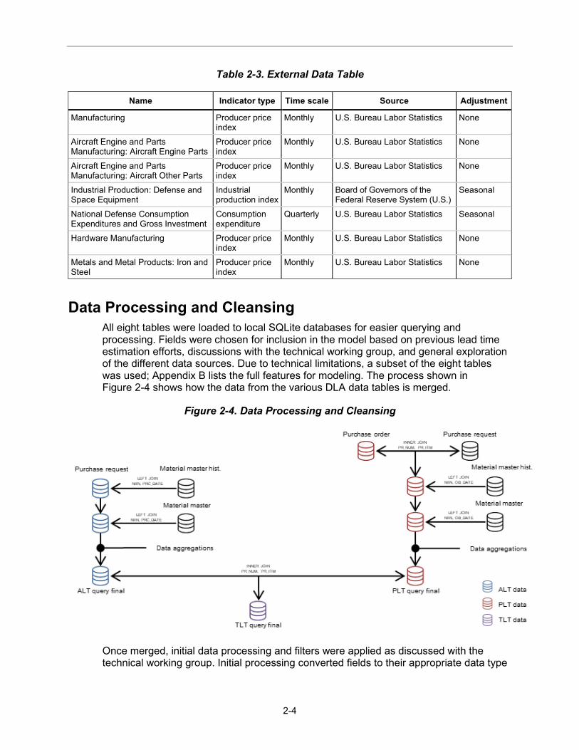
All eight tables were loaded to local SQLite databases for easier querying and processing. Fields were chosen for inclusion in the model based on previous lead time estimation efforts, discussions with the technical working group, and general exploration of the different data sources. Due to technical limitations, a subset of the eight tables was used; Appendix B lists the full features for modeling. The process shown in Figure 2-4 shows how the data from the various DLA data tables is merged.

Figure 2-4. Data Processing and Cleansing

Once merged, initial data processing and filters were applied as discussed with the technical working group. Initial processing converted fields to their appropriate data type

Technical Approach

2-5

(e.g., obligation date is converted to a datetime field) for easier data manipulation. The initial filters removed records that satisfied at least one of three criteria:

• Alphanumeric Material Numbers—The working group decided to omit predictions of lead times for these broad and/or non-DLA managed Material Numbers (leaving only NIINs): As a result, Material Numbers with six prefixes are removed: GM (non-National Stock Number items), LL (Navy Managed Supply Items), LN (local buys), N (DLA Disposition Services Items), S (Service Material), F (Local Controlled Inventory Number).

• Long-term contracts (LTCs)—Identified by the ninth digit of the Procurement Instrument Identification Number (PIIN). LTC lead times are expected to behave differently and should, therefore, be modeled separately.

• Records with missing values for procurement date or document date (for ALT) or obligation date or delivery date (for PLT)—without these date values, the observed ALT or PLT cannot be calculated.

Because our models predict at the NIIN level—not the PO or PR level—the data is grouped by PR number and NIIN (for ALT modeling data); PO number and NIIN (for PLT modeling data); or PR number, PO number, and NIIN (for TLT modeling data) with the other fields aggregated in a logical fashion to create a single row for each unique combination. For each combination, aggregation methods include taking the sum or mean of numeric fields (e.g., summing the delivered quantity for a PO and NIIN to calculate the total delivered quantity) or taking the first or last of categorical fields (e.g., using the first chronological document type for a PO and NIIN to get the first item category). Appendix C lists the full rules for procurement-level aggregation.

Although an actual delivery date exists in the PO table, the delivery date used to mark the end of PLT is a calculated date field based on discussions with the technical working group. The delivery date for a unique combination of PO number and NIIN is when more than 50 percent of the total delivered quantity of that PO number and NIIN has been delivered. The observed (actual) PLT is calculated by subtracting the obligation date from the delivery date.

A hypothetical example (see Figure 2-5) demonstrates some of the calculations that create the final (PLT) modeling data with the new procurement-level aggregation fields in italics (the original fields are then dropped as well as any resulting duplicate rows).

2-6

Figure 2-5. Example of Procurement-Level Data Aggregations

Final filtering and processing were applied to data following discussions with the technical working group. The final processing step replaced null values in categorical fields with a default “empty_value” for use by the model. The final filtering step removed records that satisfied at least one of two criteria:

• Observed ALT or PLT of 0 days—These are likely errors or the result of automated purchases not intended for inclusion in this modeling effort.

• Numeric fields with null values—Unlike the categorical fields, no natural default value can be used.

Feature Engineering Feature engineering creates new or derivative features from processed and cleaned DLA data. Appendix B describes the engineering process and the full list of engineered features. New features can be categorized as historical aggregations of raw features, date component features, and novel features. Many new features were re-engineered based on previous work on lead time estimation.1F

1

Historical Aggregations of Features At the time of inference, when a lead time prediction is made for an NIIN, the goal is to predict the time it will take for the next PR to be awarded, or the next PO to be delivered. For the NIIN, the feature values from the PO and PR table are not available, because the PR has not been generated and the PO has not been awarded. This constraint poses significant issues for models trained on historical data where raw feature values from PO and PR tables are available for model training, but unavailable at inference time. To get around this problem, historical aggregation features substitute for raw features from PO and PR tables. These features are the mean, median, mode, or sum of the previous n delivery months’ raw feature values (award months, if modeling for ALT or TLT). The value of n can range from 1 to 10. Setback features, another variant of historical aggregates, are combined over the second, third, or fourth previous delivery or

1 Michael D. Bosack et al., Production Lead Time Estimation, DL304T4 (Tysons, VA: LMI, July 2016).

Purchase order # NIIN Delivered

quantityItem

categoryObligation

dateActual

delivery date

1525354555 012345678 20 A 10/1/2007 10/1/2009

1525354555 012345678 10 B 10/1/2007 11/1/2009

1525354555 987654321 30 A 10/1/2006 1/1/2010

Purchase order # NIIN

Total delivered quantity

First item category

Obligation date

Delivery date

Observed PLT

1525354555 012345678 30 A 10/1/2007 10/1/2009 731

1525354555 987654321 10 A 10/1/2007 1/1/2010 823

Technical Approach

2-7

award month. Historical aggregate features supply valuable information on the historical trends of raw features and replace raw PO and PR features unavailable at inference time.

Figure 2-6 depicts an example calculation of a historical aggregate feature. The original feature value (delivery quantity) is shown in the left table, while the historical aggregation of the original feature value over the past award month is shown in the right table. Color bands indicate which original delivery quantity records from previous award months create corresponding records in the aggregated delivery quantity field.

Figure 2-6. Example of Historical Aggregation Engineered Feature

Date-Derived Features Date-derived features are derivatives of raw date features. For example, procurement date month-year is the month-year component of the full procurement date feature, supplying the exact date an item is procured. Integer document date converts document dates into an ordinal integer format. Date-derived features help capture the seasonality in raw date values.

Novel Features Novel features are new features created in response to working group discussions with DLA. Examples include days-since-last-procurement (a measure of the number of days elapsed since an NIIN was last procured) and profit center workload (a measure of the number of open procurements being worked by an NIIN’s profit center).

Figure 2-7 depicts the profit center workload calculation. For any item, the collection of item records that share that item’s profit center are compiled into small dataset. Profit center workload is calculated on this dataset as the number of item records that have procurement windows which overlap with the item’s procurement date.

Proc. date

Award date

Delivery qty

1/18 1/18 10

2/18 3/18 20

2/18 3/18 30

4/18 5/18 10

4/18 5/18 50

6/18 7/18 10

Proc. date Aggregated delivery qty

1/18 0

2/18 10

2/18 10

4/18 25

4/18 25

6/18 30

Original feature table Historically aggregated feature table

0 default value when no previous award month found

(20 + 30) ÷ 2 = 25

(10 + 50) ÷ 2 = 30

2-8

Figure 2-7. Profit Center Workload

Feature Engineering by Estimation Task Though most engineered features are used in both ALT and PLT estimation, slight variations in engineering functions tailor features for each lead time estimation task. In addition, certain features are exclusively for ALT estimation or PLT estimation. Feature engineering for TLT estimation takes a selection from ALT and PLT engineered features.

In ALT estimation, historical aggregate features are derived by calculating aggregations over PRs awarded (document date) before the PR is opened (procurement date). An example of this type of calculation can be found in the Historical Aggregations of Features section. The ALT of record (ALTR) and observed ALT are used for features requiring previously observed and lead time of record values. PR-specific information, such as PR doctypes and PR price, furnish data for several custom ALT features.

In PLT estimation, historical aggregate features are derived by calculating aggregations over POs delivered (delivery date) before the PO is awarded (obligation date). The PLT of record (PLTR) and observed PLT are used for features requiring previously observed and lead time of record values. PO-specific information, such as PO doctypes and delivery quantity, supply data for several custom PLT features.

In TLT estimation, historical aggregate features are derived by calculating aggregations over procurements delivered (delivery date) before the procurement is opened (procurement date). The sum of ALTR and PLTR is used for features requiring total lead time of record (TLTR). The sum of observed ALT and PLT is used for features requiring previously observed lead time.

Appendix B lists all engineered features by estimation task.

Encoding and Scaling Encoding transforms categorical variables into numerical variables that can be interpreted by ML algorithms. One-hot encoding transforms all categorical variables. When a categorical variable is one-hot encoded, a new binary variable is created for each of the unique values. Figure 2-8 is an example of one-hot encoding the categorical variable first article test (FAT) indicator that has two unique values: Y and N. After one-hot encoding, the original categorical variable is replaced with two binary variables: FAT_Y and FAT_N. Each record has a 1 in the column for the binary variable corresponding to its original value and a 0 in the other.

Technical Approach

2-9

Figure 2-8. One-Hot Encoding Example

Each categorical feature is replaced by multiple one-hot encoded features, one for each unique feature value. As a result, one-hot encoding is prone to feature explosion, especially for features with high cardinalities. To avoid feature explosion, a binning process discards rare values of features. For all lead time estimation datasets, a rarity threshold of 2,500 is set for binning. Before the encoding step, each feature is examined and values that appear in less than 2,500 records are binned into the generic category “RARE_VALUE.” Binning reduces the unique values per feature, decreasing one-hot encoded features and keeping the dataset in reasonable memory limits. While binning decreases the diversity of values for certain features, the effects of binning feature values comprising 2,500 records or less (<1 percent of records for any lead time dataset) are negligible when assessing model accuracy.

After encoding, standard scaling—meant to improve convergence time for gradient descent algorithm—centers the distribution of numeric feature values near 0 with a standard deviation of 1.

Encoding and scaling are conducted prior to splitting the data for train and test, with negligible risk of data snooping since train-test splits have similar distributions of feature values.

Model Training Once data cleansing, feature engineering, and encoding and scaling are complete, the data is ready to train ML models. Figure 2-9 depicts the training process, with an ML model learning from the data, and the corresponding observed lead times. Each row in the training data corresponds to a unique lead time observation. For ALT, each row is a unique PR-NIIN pair; for PLT, each row is a unique PR-NIIN pair; and for TLT, each row is a unique PR-PO-NIIN triple.

Figure 2-9. Model Training (ALT Example)

The trained AI model can predict lead times, as shown in Figure 2-10. The AI model is then evaluated by generating predictions for the test data and comparing those predictions to the observed lead time values.

Record # FAT indicator

1 Y

2 N

Record # FAT_Y FAT_N

1 1 0

2 0 1

One-hot encoding

ALT AI model

Model data(1 row per PR-NIIN)

Observed ALT(1 row per PR-NIIN)

Model training

2-10

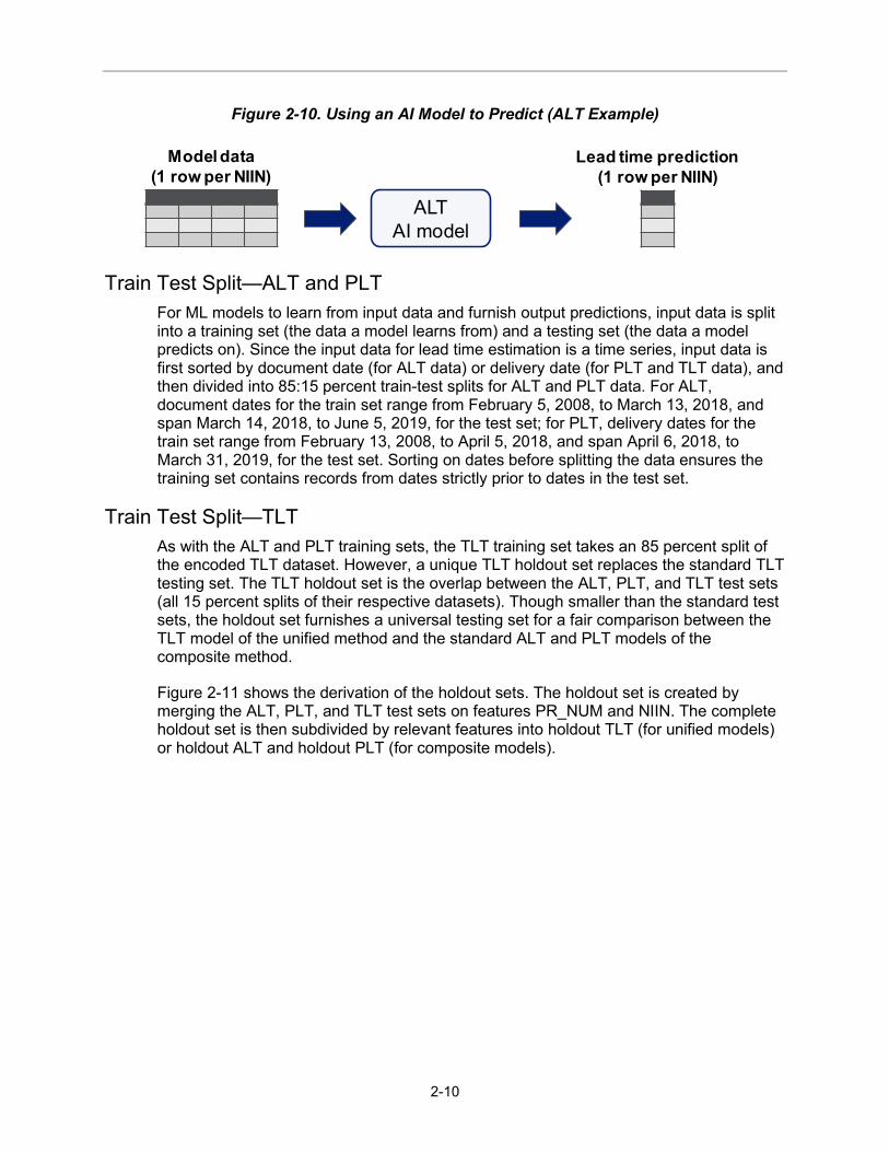
Figure 2-10. Using an AI Model to Predict (ALT Example)

Train Test Split—ALT and PLT For ML models to learn from input data and furnish output predictions, input data is split into a training set (the data a model learns from) and a testing set (the data a model predicts on). Since the input data for lead time estimation is a time series, input data is first sorted by document date (for ALT data) or delivery date (for PLT and TLT data), and then divided into 85:15 percent train-test splits for ALT and PLT data. For ALT, document dates for the train set range from February 5, 2008, to March 13, 2018, and span March 14, 2018, to June 5, 2019, for the test set; for PLT, delivery dates for the train set range from February 13, 2008, to April 5, 2018, and span April 6, 2018, to March 31, 2019, for the test set. Sorting on dates before splitting the data ensures the training set contains records from dates strictly prior to dates in the test set.

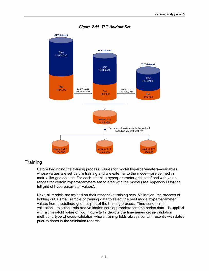
Train Test Split—TLT As with the ALT and PLT training sets, the TLT training set takes an 85 percent split of the encoded TLT dataset. However, a unique TLT holdout set replaces the standard TLT testing set. The TLT holdout set is the overlap between the ALT, PLT, and TLT test sets (all 15 percent splits of their respective datasets). Though smaller than the standard test sets, the holdout set furnishes a universal testing set for a fair comparison between the TLT model of the unified method and the standard ALT and PLT models of the composite method.

Figure 2-11 shows the derivation of the holdout sets. The holdout set is created by merging the ALT, PLT, and TLT test sets on features PR_NUM and NIIN. The complete holdout set is then subdivided by relevant features into holdout TLT (for unified models) or holdout ALT and holdout PLT (for composite models).

Model data(1 row per NIIN)

Lead time prediction(1 row per NIIN)

ALTAI model

Technical Approach

2-11

Figure 2-11. TLT Holdout Set

Training Before beginning the training process, values for model hyperparameters—variables whose values are set before training and are external to the model—are defined in matrix-like grid objects. For each model, a hyperparameter grid is defined with value ranges for certain hyperparameters associated with the model (see Appendix D for the full grid of hyperparameter values).

Next, all models are trained on their respective training sets. Validation, the process of holding out a small sample of training data to select the best model hyperparameter values from predefined grids, is part of the training process. Time series cross-validation—to select train and validation sets appropriate for time series data—is applied with a cross-fold value of two. Figure 2-12 depicts the time series cross-validation method, a type of cross-validation where training folds always contain records with dates prior to dates in the validation records.

Test~464,000

Train~2,634,000

Train

Test~380,000

Train

Test~282,000

Train~2,156,386

Train~1,602,000

Holdout set~184,000

Holdout PLT~184,000

Holdout ALT~184,000

Holdout TLT~184,000

INNER JOINPR_NUM, NIIN


For each estimation, divide holdout set based on relevant features

ALT dataset

PLT dataset

TLT dataset

2-12

Figure 2-12. Time Series Cross-Validation

Four types of ML models generated predictions: decision tree (DT), random forest (RF), linear regression (LR), and neural network (NN) (see Appendix E for model descriptions). All models are instantiated through the scikit-learn Python library (see Appendix A for software version details). Each model has advantages and disadvantages; Table 2-4 states the general tradeoffs between models.

Table 2-4. ML Model Tradeoffs

Model Pros Cons

DT • Can capture certain non-linear relationships • Easy to derive feature importance • Easily interpretable through visualization

• Causes prediction banding for regression problems • Prone to overfit

RF • Can capture most non-linear relationships • Ensemble method provides higher accuracy • Easy to derive feature importance

• Causes prediction banding for regression problems • Higher computational cost than DTs • Less interpretable than DTs

LR • Simplest model to implement • Easy to derive feature importance

• Cannot capture nonlinear relationships • Computationally easy

NN • Can capture most non-linear relationships • High accuracy for problems with lots of data

• Hard to explain • Hard to interpret • Computationally intensive

Model Evaluation The test sets defined in the previous section are used to evaluate and compare various methods for estimating lead times. Baseline forecasting methods improved by AI models and evaluation metrics are described below.

Baseline Forecasting Methods Each of the ML models are compared to two baseline forecasting methods: lead time of record and one-third rule. Comparing model results against a baseline evaluates whether the ML models offer additional value over DLA’s current forecasting methods.

ALTR, PLTR, and TLTR: pulled from historical data, ALTR and PLTR are the lead time estimates on record at DLA at the time a PR is generated (ALTR) or a PO is awarded (PLTR). This baseline furnishes a comparison to the lead time forecasts of DLA planners and incorporates manual overrides, forecast freezes, or changes in forecasting methods over time.

One-third rule: an exponential smoothing method with an alpha of one-third. At the end of each month, the lead time forecast is updated:

𝑓𝑓𝑓𝑓𝑓𝑓𝑓𝑓𝑓𝑓𝑓𝑓𝑓𝑓𝑓𝑓𝑡𝑡 =13

(𝑓𝑓𝑎𝑎𝑓𝑓𝑓𝑓𝑓𝑓𝑎𝑎𝑓𝑓 𝑓𝑓𝑜𝑜𝑓𝑓𝑓𝑓𝑓𝑓𝑎𝑎𝑓𝑓𝑜𝑜 𝑙𝑙𝑓𝑓𝑓𝑓𝑜𝑜 𝑓𝑓𝑡𝑡𝑡𝑡𝑓𝑓 𝑓𝑓𝑓𝑓𝑓𝑓𝑡𝑡 𝑡𝑡𝑓𝑓𝑚𝑚𝑓𝑓ℎ 𝑓𝑓) + 23

(𝑓𝑓𝑓𝑓𝑓𝑓𝑓𝑓𝑓𝑓𝑓𝑓𝑓𝑓𝑓𝑓𝑡𝑡−1).

Test

Test

Validation

ValidationTrain

Train

Technical Approach

2-13

By computing the one-third rule from the procurement data, the effects of manual overrides, forecast freezes, or changes in the alpha value over time are removed.

Evaluation Metrics Per our discussion with DLA, several metrics evaluate how well our final models performed, with minimizing mean absolute error (MAE) as the primary goal and minimizing mean absolute percentage error (MAPE) as the secondary goal. Appendix F includes additional discussion of metrics.

MAE: Measures a model’s raw error by averaging the absolute errors across all observations.

MAPE: Measures a model’s magnitude of error by averaging the absolute percentage of errors across all observations.

3-1

Analysis and Results

ALT and PLT Predictive Models Model performance is compared by procurement frequencies and the direction of errors. Appendix D catalogs the complete ALT and PLT model parameters and scores.

Overall Results Table 3-1 lists the overall scores for MAE and MAPE for baseline measures and ML models evaluated on the ALT and PLT test sets.

Table 3-1. Overall ALT and PLT Model Scores

ALT model scores PLT model scores

Model MAE

(days) Standard

error MAPE

(%) Standard

error

Model MAE

(days) Standard

error MAPE

(%) Standard

error

RF 37 0.10 86 0.29 RF 67 0.22 142 0.63 DT 39 0.10 234 0.83 DT 68 0.22 142 0.64 LR 38 0.11 136 0.51 LR 72 0.22 109 0.50 NN 42 0.11 280 0.84 NN 72 0.22 153 0.67 ALT one-third rule

53 0.11 386 1.22 PLT one-third rule

83 0.24 229 1.19

ALTR 56 0.12 448 1.37 PLTR 94 0.25 286 1.52 Baseline Scores

The one-third rule is, on average, 3 days and 62 percentage points closer to predicting the true ALT than the ALTR baseline. The one-third rule is, on average, 11 days and 57 percentage points closer to predicting the true PLT than the PLTR baseline. The one-third rule performs better than the lead time of record in both cases. This indicates that manual overrides and freezes hurt the accuracy of lead time predictions.

ML Model Scores AI models produce significantly better scores than baseline results for ALT and PLT. RF is the most accurate model for ALT and PLT, reducing MAE for both ALT and PLT by 16 days compared to the one-third rule.

The higher MAEs for PLT and the higher MAPEs for ALT reflect the differences in the distributions of observed ALT and PLT. The observed ALT test set has a range of 1–2,344 with a mean of 50 and a median of 18 while the observed PLT test set has a range of 1–3,878 with a mean of 115 and a median of 73. The predicted values have similar distributions so the smaller values for ALT result in smaller absolute errors and larger absolute percent errors.

3-2

Procurement Frequency Breakdown The baseline DLA forecasting methods perform well on frequently procured items, since these items experience less lead time variability. The baseline methods perform poorly on infrequently procured items since those items experience more lead time variability. One of the primary advantages of ML models is that they can learn from other similar items with more recent lead time observations when making a prediction for infrequently procured items.

To compare how each model performs for infrequently procured items, we compute the procurement frequency for each item in each of the test datasets, using seven procurement frequency categories: monthly, quarterly, twice a year, yearly, every 2 years, rare, and one-time buy. The procurement data ranges from February 2007 to June 2019, spanning 148 months, 49 quarters, etc. An item was categorized as monthly if it had at least 148 procurement records, quarterly if it had between 49 and 148 records, and so on. Figure 3-1 shows the percentage of NIINs that fall into each procurement frequency category. Though not displayed, the PLT test set, which uses obligation date instead of procurement date for frequency, follows a similar distribution, with the vast majority of NIINs procured, at most, every 2 years.

Figure 3-1. ALT Test Set Procurement Frequency Distribution

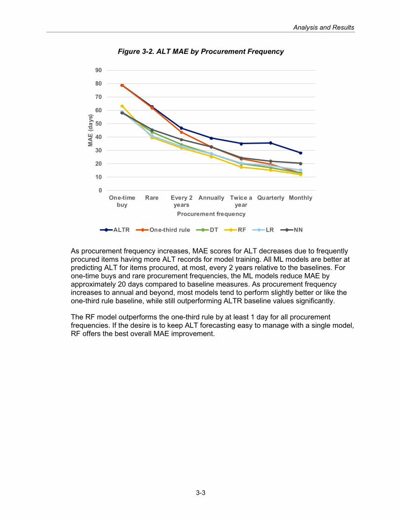
An item’s procurement frequency is driven by demand and, therefore, out of DLA’s control. However, DLA can monitor an item’s procurement frequency and use that value to evaluate which forecasting method to use. Figure 3-2 shows the breakdown of baseline and model results for ALT by procurement frequency.

2.7% 2.8% 3.2%

10.7%

25.3%

43.0%

12.4%

0%

10%

20%

30%

40%

50%

Monthly Quarterly Twice ayear

Annually Every 2years

Rare One-timebuy

NIIN

s



3-3

Figure 3-2. ALT MAE by Procurement Frequency

As procurement frequency increases, MAE scores for ALT decreases due to frequently procured items having more ALT records for model training. All ML models are better at predicting ALT for items procured, at most, every 2 years relative to the baselines. For one-time buys and rare procurement frequencies, the ML models reduce MAE by approximately 20 days compared to baseline measures. As procurement frequency increases to annual and beyond, most models tend to perform slightly better or like the one-third rule baseline, while still outperforming ALTR baseline values significantly.

The RF model outperforms the one-third rule by at least 1 day for all procurement frequencies. If the desire is to keep ALT forecasting easy to manage with a single model, RF offers the best overall MAE improvement.

0

10

20

30

40

50

60

70

80

90

One-timebuy

Rare Every 2years


Quarterly Monthly

MAE

(day

s)


ALTR One-third rule DT RF LR NN

3-4

Figure 3-3. ALT MAPE by Procurement Frequency

As procurement frequency increases, MAPE scores for ALT increase for all prediction methods, except the one-third rule. An increase in MAPE for ALTR and NN for monthly, quarterly, and biannual procurements is observed due to the shorter observed lead times for frequently procured items. With shorter lead times, small differences between true and predicted values result in large percentage errors as true values decrease in magnitude.

Overall, RF offers the best MAPE scores for all procurement frequencies of ALT. In addition, RF has the most consistent MAPE values across all procurement frequency categories. Combined with the MAE procurement frequency from an item’s procurement frequency is driven by demand and, therefore, out of DLA’s control. However, DLA can monitor an item’s procurement frequency and use that value to evaluate which forecasting method to use. Figure 3-2 shows the breakdown of baseline and model results for ALT by procurement frequency, these results strengthen the conclusion that RF should be the overall ALT model.

As procurement frequency increases, MAE scores for PLT first decrease slowly until the frequency increases past annual procurements, after which, most MAE scores decrease quickly (see Figure 3-4) due to frequently procured items having more PLT records for model training. All models are better at predicting PLT for rare and one-time buy items relative to baseline results for the same frequency categories. For one-time buys, the highest performing model, RF, reduces MAE by approximately 44 days compared to baseline measures. As procurement frequency increases to every 2 years and beyond, LR and DT tend to perform like the one-third rule baseline, while outperforming PLTR baseline values significantly.

0100200300400500600700800900

1,000

One-timebuy

Rare Every 2years


Quarterly Monthly

MAP

E (%

)




3-5

Figure 3-4. PLT MAE by Procurement Frequency

For PLT, the ML models reduce MAE only for rare and one-time buys. This suggests that DLA should set a procurement frequency threshold of every 2 years to evaluate whether to forecast an item’s PLT using the one-third rule or an ML model.

Figure 3-5. PLT MAPE by Procurement Frequency

0

20

40

60

80

100

120

140

One-timebuy

Rare Every 2years


Quarterly Monthly

MAE

(day

s)


PLTR One-third rule DT RF LR NN

0

100

200

300

400

500

600

One-timebuy

Rare Every 2years


Quarterly Monthly

MAP

E (%

)



3-6

As procurement frequency increases, MAPE for PLT decreases until annual procurements, after which MAPE increases with twice a year, quarterly, and monthly procurements due to the shorter observed lead times for frequently procured items. With shorter lead times, small differences between true and predicted values result in large percentage errors as true values decrease in magnitude.

LR furnishes the best MAPE scores for the most procurement frequencies of PLT, followed by RF. Both improve on the one-third rule for all procurement frequencies. Since MAE scores are used as the primary metric to compare performance between models, the scores from both figures suggest that RF should be the PLT forecasting method for infrequently procured items.

Overall, ML models offer the biggest opportunities for improvement for infrequently procured items for ALT and PLT.

Direction of Error Prediction errors can be underestimates or overestimates. Error direction, in the context of lead time estimation, has differing consequences: underestimates lead to lower availability and higher backorder, whereas overestimates lead to overstocking and higher holding costs. Depending on DLA business priorities, the direction of a model’s error may help evaluate which model to use for lead time estimation. In addition, the magnitude of the error is also important. A 1-day underestimate may be preferred to a 30-day overestimate. Figure 3-6 and Figure 3-7 show the magnitude and direction of errors for ALT and PLT models.

Figure 3-6. ALT Magnitude and Direction of Errors

0%

10%

20%

30%

40%

50%

60%

70%

80%

90%

100%


Tota

l rec

ords

Model

> 6 months over

> 1 month over

> 7 days over

± 7 days

> 7 days under

> 1 month under

> 6 months under


3-7

For ALT, both baseline models tend to overpredict (blue bars) more than underpredict (red bars). Over 60 percent of records are overpredicted by more than 7 days, and 40 percent of records are overpredicted by at least 1 month. This tendency to overpredict could lead to overinvestments in on-hand inventory. In contrast, the ML models reduce the number of overestimates, especially large overestimates, and increase the number of estimates that are within 7 days of the true lead time. However, this improvement corresponds with an increase in underestimates.

Figure 3-7. PLT Magnitude and Direction of Error

For PLT, both baseline models tend to overpredict more than underpredict. Close to 60 percent of records are overpredicted by more than 7 days, and over 40 percent of records are overpredicted by at least 1 month. This overprediction could lead to overinvestments in on-hand inventory. See Appendix G for an exploration of padding the RF model to match the baseline direction of error distribution better.

The ML models all reduce the number of PLT overestimates and nearly eliminate all overestimates larger than 6 months. As with ALT, the ML models increase underestimates, bringing the ratio of over- to underestimates closer to 50–50.

Feature Insight Although AI models do not evaluate causal relationships between the various features and lead times, the models offer some feature insights. For tree-based models (DT and RF), feature importance finds the features that contribute the most to the accuracy of the model, based on the chosen loss function, to train the model. The loss function for tree-based models is mean squared error (MSE): features that improve MSE of the model as

0%

10%

20%

30%

40%

50%

60%

70%

80%

90%

100%


Tota

l rec

ords

Model

> 6 months over

> 1 month over

> 7 days over

± 7 days

> 7 days under

> 1 month under

> 6 months under

3-8

a whole are more important. Note that the loss function is an optimization metric—meant to maximize the accuracy of a single model—and not an evaluation metric, which compares across models. Appendix F details the metrics.

Feature importance explains which features contribute the most to the accuracy of model predictions. Appendix E contains a more detailed description of feature importance. In addition, feature importance identifies the features where data accuracy is most important. For example, since features with high importance contribute so much to model accuracy, it is crucial that any bias or quality issues of those features be resolved.

Linear models furnish a different type of feature insight. Instead of quantifying the predictive power of each feature in a model, LR generates coefficients for each individual feature, which measures how that feature impacts the predicted value itself. Feature impact is measured by the absolute value of the coefficient; features marked with “(−)” in the subsequent figures denote a negative coefficient value; that is, an increase in feature value lowers the lead time.

NNs’ complexity makes the contribution of each feature difficult to evaluate and less apparent.

ALT Several of the features that contribute the most to the DT model’s accuracy relate to time (see Figure 3-8). Months since last award is the number of months since the last document date of an NIIN. Days since last procurement is the days since the last procurement date of an NIIN. Procurement date as integer is a numeric translation of the date on which the prediction is made. This finding aligns with the working group’s intuition since it may be harder to find a supplier if it has been a long time since the NIIN was procured. Though feature importance does not indicate how months since last award may affect lead time, it does indicate that the feature greatly improves model accuracy, so the relationship is significant. PR count by demilitarization code is second in importance, showing that the number of requisitions for a single demilitarization code may influence lead time predictions.


3-9

Figure 3-8. ALT DT Top 10 Important Features

The RF model shares 7 of the top 10 most important features with the DT model, though the order is different (see Figure 3-9). The two P9 mode features (V = purchase orders—automated and M = purchase orders—manual) have been swapped for record count and mean ALT, while common award type has flipped from manual to automated. This similarity is not surprising; RF can be thought of as a collection of small DTs whose results are averaged together. The top feature in both, however, remains months since last award.

Figure 3-9. ALT RF Top 10 Important Features

0 0.1 0.2 0.3 0.4

P9 mode (1M lookback): M

Two-third rule

Median ALT by profit center

Common doctype (10M lookback): ZRLP

P9 mode (10M lookback): V

Days since last procurement

Procurement date as integer

Common award type: MANUAL

PR count by demilitarization code

Months since last award

Feature importance

Feat

ure

nam

e

0 0.1 0.2 0.3

Common doctype (10M lookback): ZRLP

Mean ALT

PR count by demilitarization code

Record count


Two-third rule

Common award type: AUTOMATED

Days since last procurement

Procurement date as integer


Feature importance

Feat

ure

nam

e

3-10

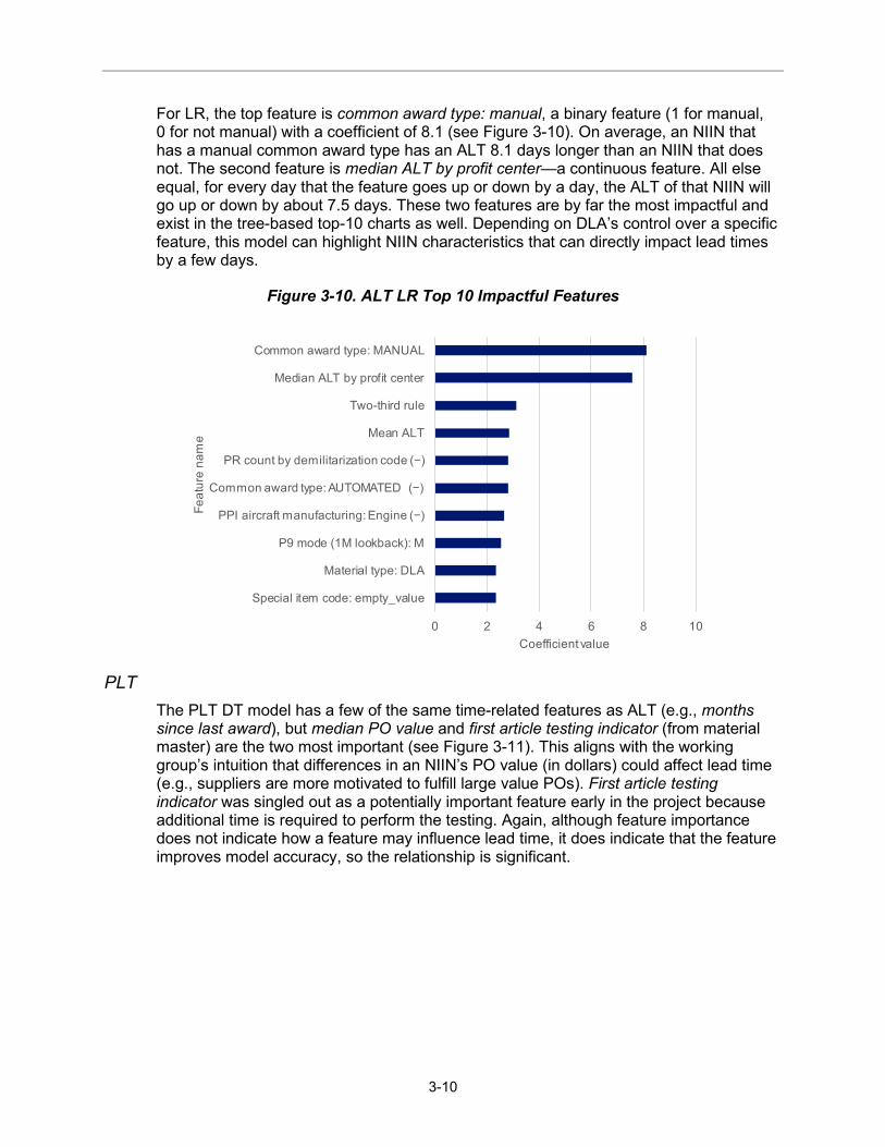
For LR, the top feature is common award type: manual, a binary feature (1 for manual, 0 for not manual) with a coefficient of 8.1 (see Figure 3-10). On average, an NIIN that has a manual common award type has an ALT 8.1 days longer than an NIIN that does not. The second feature is median ALT by profit center—a continuous feature. All else equal, for every day that the feature goes up or down by a day, the ALT of that NIIN will go up or down by about 7.5 days. These two features are by far the most impactful and exist in the tree-based top-10 charts as well. Depending on DLA’s control over a specific feature, this model can highlight NIIN characteristics that can directly impact lead times by a few days.

Figure 3-10. ALT LR Top 10 Impactful Features

PLT The PLT DT model has a few of the same time-related features as ALT (e.g., months since last award), but median PO value and first article testing indicator (from material master) are the two most important (see Figure 3-11). This aligns with the working group’s intuition that differences in an NIIN’s PO value (in dollars) could affect lead time (e.g., suppliers are more motivated to fulfill large value POs). First article testing indicator was singled out as a potentially important feature early in the project because additional time is required to perform the testing. Again, although feature importance does not indicate how a feature may influence lead time, it does indicate that the feature improves model accuracy, so the relationship is significant.

0 2 4 6 8 10

Special item code: empty_value

Material type: DLA

P9 mode (1M lookback): M

PPI aircraft manufacturing: Engine (−)

Common award type: AUTOMATED (−)

PR count by demilitarization code (−)

Mean ALT

Two-third rule


Common award type: MANUAL

Coefficient value

Feat

ure

nam

e


3-11

Figure 3-11. PLT DT Top 10 Important Features

The RF model shares 9 of the top 10 most important features with the DT model, though the order is different. One-third rule has been swapped for item category: 0 (which is the standard). Given similarities in how DT and RF models work, the similarities are foreseeable. The top four are the same (see Figure 3-12).

Figure 3-12. PLT RF Top 10 Important Features

For LR, the top feature is item category: 0, a binary feature that denotes whether an NIIN is in the standard item category or not (see Figure 3-13). On average, an NIIN in this item category has a PLT 10 days longer than an NIIN that does not. Although some

0 0.1 0.2 0.3 0.4 0.5

One-third rule (3M lookback)

Acquisition method suffix Code: G

Item category: 5

Obligation date as integer

One-third rule

Obligation date month year: RARE_VALUE


Two-third rule

First article testing ind. (material master)

Median PO value (10M lookback)

Feature importance

Feat

ure

nam

e

0 0.1 0.2 0.3 0.4 0.5

Item category: 0

One-third rule (3M lookback)

Item category: 5

Acquisition method suffix code: G

Obligation date as integer

Obligation date month year: RARE_VALUE


First article testing ind. (material master)

Two-third rule

Median PO value (10M lookback)

Feature importance

Feat

ure

nam

e

3-12

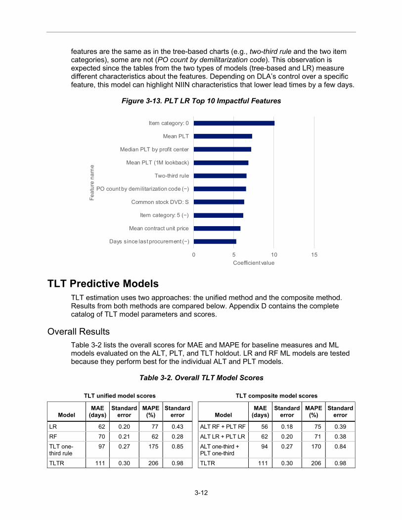
features are the same as in the tree-based charts (e.g., two-third rule and the two item categories), some are not (PO count by demilitarization code). This observation is expected since the tables from the two types of models (tree-based and LR) measure different characteristics about the features. Depending on DLA’s control over a specific feature, this model can highlight NIIN characteristics that lower lead times by a few days.

Figure 3-13. PLT LR Top 10 Impactful Features

TLT Predictive Models TLT estimation uses two approaches: the unified method and the composite method. Results from both methods are compared below. Appendix D contains the complete catalog of TLT model parameters and scores.

Overall Results Table 3-2 lists the overall scores for MAE and MAPE for baseline measures and ML models evaluated on the ALT, PLT, and TLT holdout. LR and RF ML models are tested because they perform best for the individual ALT and PLT models.

Table 3-2. Overall TLT Model Scores

TLT unified model scores TLT composite model scores

Model MAE

(days) Standard

error MAPE

(%) Standard

error

Model MAE

(days) Standard

error MAPE

(%) Standard

error

LR 62 0.20 77 0.43 ALT RF + PLT RF 56 0.18 75 0.39 RF 70 0.21 62 0.28 ALT LR + PLT LR 62 0.20 71 0.38 TLT one-third rule

97 0.27 175 0.85 ALT one-third + PLT one-third

94 0.27 170 0.84

TLTR 111 0.30 206 0.98 TLTR 111 0.30 206 0.98

0 5 10 15

Days since last procurement (−)

Mean contract unit price

Item category: 5 (−)

Common stock DVD: S

PO count by demilitarization code (−)

Two-third rule

Mean PLT (1M lookback)

Median PLT by profit center

Mean PLT

Item category: 0

Coefficient value

Feat

ure

nam

e


3-13

Baseline Scores The one-third rule is, on average, 14 days and 31 percentage points closer to predicting the true TLT than the TLTR baseline.

ML Model Scores Both unified and composite TLT AI models produce significantly better scores than both baseline results. Composite RF is the most accurate, reducing MAE by 38 days and MAPE by 95 percentage points compared to the composite one-third rule.

Since DLA uses the ALT and PLT components of lead time separately, two models are required. An additional TLT unified model would be useful only if it supplies additional improvements over the composite model; however, that benefit is not demonstrated in these results.

Procurement Frequency Breakdown Figure 3-14 shows a breakdown of TLT baseline and model results by procurement frequency.

Figure 3-14. TLT MAE by Procurement Frequency

Baseline MAE scores decrease from one-time buy procurements to annual procurements, after which they increase for TLTR while continuing to slowly decrease for the one-third rule.

All TLT AI models are better at predicting TLT for items procured, at most, every 2 years relative to the baselines. As procurement frequency increases to annual and beyond, most models produce MAE’s similar or slightly worse than the one-third rule baseline

0

20

40

60

80

100

120

140

160

One-timebuy

Rare Every 2years


Quarterly Monthly

MAE

(day

s)


TLTR One-third rule RFLR ALT RF + PLT RF ALT LR + PLT LR

3-14

(except composite RF, which performs slightly better) while still outperforming TLTR baseline values significantly. The composite RF model performs the best across nearly all procurement frequencies, with the unified RF model performing slightly better for quarterly and monthly items.

Baseline MAPE scores decrease from one-time buy procurements to annual procurements, after which they increase for TLTR while continuing to slowly decrease for the one-third rule (see Figure 3-15). An increase in MAPE for TLTR for quarterly procurements is observed due to the shorter observed lead times for frequently procured items. With shorter lead times, small differences between true and predicted values result in large percentage errors as true values decrease in magnitude.

Figure 3-15. TLT MAPE by Procurement Frequency

Like MAE, all TLT models score significantly better MAPEs for items procured, at most, every 2 years relative to the baselines. As procurement frequency increases to annual and beyond, all models continue to produce MAPEs better than the one-third rule baseline to a smaller degree. The unified and composite models perform similarly for MAPE scores.

Direction of Error Figure 3-16 shows the magnitude and direction of error for all TLT models.

0

50

100

150

200

250

300

One-timebuy

Rare Every 2years


Quarterly Monthly

MAP

E (%

)


TLTR One-third rule RFLR ALT RF + PLT RF ALT LR + PLT LR


3-15

Figure 3-16. TLT Magnitude and Direction of Error

Both baseline models tend to overpredict more than underpredict. Approximately 70 percent of records are overpredicted by more than 7 days, and 60 percent of records are overpredicted by at least 1 month. This overprediction could lead to overinvestments in inventory.

Both the unified and composite models are skewed toward underestimates, which could lead to an increase in backorders. On the other hand, the AI models nearly eliminate overestimates longer than 6 months and greatly reduce overestimates longer than 1 month, reducing inventory investment.

See Appendix H for breakdowns of the magnitude and direction of error by procurement frequency.

Risk Metric Using the model results (specifically the model errors), we created a simple metric to capture the variability of previous lead time estimates for each NIIN in a manner useful to a DLA planner. The metric calculates the mean of previous positive lead time errors and the mean of previous negative lead time errors for insight into the direction of error for each NIIN. Error is predicted lead time minus observed lead time; positive error corresponds to an overestimate and negative error indicates an underestimate.

Risk is best depicted by centering on an NIIN’s current predicted lead time and then adding bars indicating mean errors (note that these are not statistical error bars). Figure 3-17 is an example using ALT RF predictions.

0%

10%

20%

30%

40%

50%

60%

70%

80%

90%

100%

TLTR One-third rule Unified RF Unified LR ALT RF + PLTRF

ALT LR + PLTLR

Tota

l rec

ords

Model

> 6 months over

> 1 month over

> 7 days over

± 7 days

> 7 days under

> 1 month under

> 6 months under

3-16

Figure 3-17. Predicted ALT (RF) with Mean Error Bars

Each blue dot represents the latest ALT RF prediction; the part of the bar below the dot indicates the mean of previous positive errors (overestimates) and the part of the bar above the dot indicates the mean of previous negative errors (underestimates). For NIIN 997834056, previous overestimates of ALT are, on average, over by 7 days and previous underestimates are, on average, under by 14 days. In addition, the length of the bar gives insight on how accurate the model has been for that NIIN; 997993094 had a few overestimates in the past but the model is generally accurate based on error magnitude.

A limitation of the metric is that the averaging of errors provides no insight into past lead times or their variability, so other aggregate functions may offer better information than average error. In addition, NIINs with few previous predictions will not benefit from the metric; if an NIIN had one previous prediction, a sample size of one makes it impossible to validate model accuracy.

This metric can add value for two primary applications:

• Manual review of outliers: the metric supplies planners with context and quick insight into model predictions. For example, NIIN 000031967 has had large underestimates; increasing the prediction would reduce backorder risk.

• Safety stock levels: the metric offers insight into variability in ALT errors. For example, safety stock could be increased for NIIN 000035607 to cover the risk due to high lead time error variability.

-20

0

20

40

60

80

100

120

000031967 000066804 000035607 997993094 997834056

Lead

tim

e (d

ays)

NIIN

4-1

Business Benefits

The business benefits for increased prediction accuracy are challenging to quantify since benefits to DLA are based on the increase in estimation accuracy and how processes are adjusted to reflect the improved accuracy. The results developed during the previous analysis assume implementation is not affected or reduced by processes. Calculating new lead times of records does not mean the lead times will be used during the procurement process automatically. The solicitation and award phases allow for flexibility in contractual delivery times for DLA and the vendor. We tracked the following metrics on the TLT test set to validate progress and success:

• Obligation authority

• Inventory storage

• Sudden changes in lead time

• Backorders.

DLA uses several methods for setting item inventory levels, which don’t all depend on lead time. For items whose levels are influenced by lead time, we expect improved lead time accuracy to improve business outcomes. Sixty-seven percent of the NIINs in the procurement data of this project fall into one of the planning categories shown in Figure 4-1.

Figure 4-1. Item Population

• Replenishment (Acquisition Advice Code [AAC] D): Lead time is used to compute the safety stock and lead time demand components of inventory levels.

• Next Gen: Lead time is a factor for computing inventory levels.

• Peak: Lead time is not directly part of computing levels. However, lead times influence the simulation metrics used to generate annual tradeoff curves, which could lead to the selection of a different operating point and, therefore, different levels.

• Non-PNG™ (Peak Policy and Next Generation™) AAC Z: Lead time is used to set minimum inventory levels.

31%

10%

17%9%

33%PeakNext GenAAC DAAC Z (excluding PNG)Other

4-2

Obligation Authority Increased lead time accuracy reduces opportunity cost due to mistimed procurements. To measure this effect, we used LMI’s Financial and Inventory Simulation Model™ (FINISIM™) to simulate a replay of the last year in our data set: April 2018 through March 2019. By measuring the change in obligations over the year, we can estimate the reduction in inventory requirements due to changing lead times.

These simulation runs require historical demand data. Although historical demand data was not part of the data received for this project, we took advantage of data we already had from various PNG™ analysis. Since this data was not available for all items, we scaled up the results to reflect the percent of items analyzed (i.e., an item was in the test set and demand data was available) versus the total project item population, by planning method. This scaling assumes that the items analyzed are a representative sample of the full item population.

The simulation results in Table 4-1 show that using the lead times from the composite RF model reduces requirements by $11 million annually. If this sample is representative, the results scale to a $102 million annual reduction in requirements for the entire item population.

Table 4-1. Requirements Reduction

Next Gen AAC D Non-PNG™ AAC Z

TLTR obligations ($M) 226 159 34 One-third rule obligations ($M) 265 155 34 ALT RF + PLT RF obligations ($M) 262 149 32 Net requirements reduction versus one-third rule (analysis sample) ($M)

3 6 2

Analysis percent of total 23% 9% 10% Scaled-up requirements reduction ($M) 13 68 21

Inventory Storage

Inventory storage is directly related to lead time requirements. The longer the lead time, the more inventory is required to cover expected sales requisitions. We can state average holding cost as a function of the cost to store an item (C), rate of demand for an item (D), safety stock kept by DLA (SS), and lead time of a given item, where lead time is the sum of PLT and ALT:

𝐴𝐴𝑎𝑎𝑓𝑓𝑓𝑓𝑓𝑓𝑎𝑎𝑓𝑓 ℎ𝑓𝑓𝑙𝑙𝑜𝑜𝑡𝑡𝑚𝑚𝑎𝑎 𝑓𝑓𝑓𝑓𝑓𝑓𝑓𝑓 = 𝐶𝐶 × �𝑆𝑆𝑆𝑆 + 𝐷𝐷×(𝐴𝐴𝐴𝐴𝐴𝐴+𝑃𝑃𝐴𝐴𝐴𝐴)2

�.

Safety stock is based on the historical uncertainty in lead time as well as several other factors, including service demand, item priority, risk assessment, complex modeling, and leadership priorities. Therefore, it is impossible to neatly separate out the portion of holding cost specifically attributable to error in lead time in DLA’s safety stock.

We can estimate the holding cost of the excess inventory required by the order’s arriving early by multiplying the cost to hold an item by the number of extra days the item needs

Business Benefits

4-3

to be held. (DLA assumes that 18 percent of an item’s procurement cost is the annual cost to hold an item, but this value is a topic of debate.) The following equation computes the holding cost for each procurement in which lead time was underestimated.

. 18365

(𝑈𝑈𝑚𝑚𝑡𝑡𝑓𝑓 𝑃𝑃𝑓𝑓𝑡𝑡𝑓𝑓𝑓𝑓)(𝑂𝑂𝑓𝑓𝑜𝑜𝑓𝑓𝑓𝑓 𝑄𝑄𝑓𝑓𝑄𝑄)(𝐷𝐷𝑓𝑓𝑄𝑄𝑓𝑓 𝑂𝑂𝑎𝑎𝑓𝑓𝑓𝑓𝑓𝑓𝑓𝑓𝑓𝑓𝑡𝑡𝑡𝑡𝑓𝑓𝑓𝑓𝑓𝑓𝑜𝑜)

Table 4-2 shows that we can expect the composite RF model to save approximately $26 million in holding cost as a result of reducing overestimated lead times. This does not include safety stock.

Table 4-2. Holding Cost Due to Overestimated Lead Times

Holding cost ($M)

TLTR (annual) 66 One-third rule (annual) 47 ALT RF + PLT RF (annual) 21 Net annual savings versus one-third rule (analysis sample) 26

10-year savings at 2% discount 234

Sudden Changes in Lead Time

Sudden changes in lead times can result in multiple issues, including administrative, expedite, and reputation costs. Managing and reducing spikes in lead times is extremely important. Each month, when lead time forecasts are updated, large changes in lead times are flagged for manual review. We used the thresholds on the percent change to select the number of lead times that would be flagged for manual review in the last month of our test set, under three conditions.

1. Current method: DLA’s April 2019 forecast is compared to the March 2019 lead time of record.

2. Current method without overrides or freezes: DLA’s April 2019 is compared to DLA’s March 2019 forecast, ignoring any freezes or overrides in the lead time of record.

3. RF: the April 2019 RF forecast is compared to the March 2019 composite RF forecast.

There are separate threshold values for ALT and PLT forecast updates. Table 4-3 shows the number of lead time updates flagged for manual review for ALT and PLT under each of the three conditions. Switching to the RF models reduces the number of lead times flagged for review by 46 percent over the current method and is in line with the total number of lead times that current forecast methods would flag with no overrides or freezes.

4-4

Table 4-3. Number of Lead Time Updates Flagged for Review

ALT PLT Total

Current method 3,762 4,694 8,456 Current method without overrides/freezes 1,940 1,990 3,928 RF 3,805 744 4,549 Net change vs current method without overrides 1,865 −1,246 619

Backorders

Historically, DLA has overexaggerated lead times to minimize the risk of backorders as seen in Figure 3-6, Figure 3-7, and Figure 3-16, showing that the baseline models skew heavily toward overestimating lead times for ALT, PLT, and TLT. Using the RF models removes this artificial lead time buffer, increasing the number of lead times that are underestimated. However, just because a lead time is underestimated does not guarantee that a backorder occurs. To create a backorder, more demand must occur during the period of underestimation than is covered by safety stock.

Backorders occur for several reasons, including inaccurate demand forecasts and underestimated lead times. We compared the safety stock to the expected demand over the period of underestimation to estimate the number of units backordered due to underestimated lead times only. Safety stock (SS) and annual demand quantity (ADQ) are used to calculate the expected demand over the period of underestimation using the following equation.

𝐸𝐸𝐸𝐸𝐸𝐸𝑓𝑓𝑓𝑓𝑓𝑓𝑓𝑓𝑜𝑜 𝑜𝑜𝑓𝑓𝑓𝑓𝑏𝑏𝑓𝑓𝑓𝑓𝑜𝑜𝑓𝑓𝑓𝑓 𝑢𝑢𝑚𝑚𝑡𝑡𝑓𝑓𝑓𝑓 = max �𝐴𝐴𝐷𝐷𝑄𝑄365

(𝑜𝑜𝑓𝑓𝑄𝑄𝑓𝑓 𝑢𝑢𝑚𝑚𝑜𝑜𝑓𝑓𝑓𝑓𝑓𝑓𝑓𝑓𝑓𝑓𝑡𝑡𝑡𝑡𝑓𝑓𝑓𝑓𝑓𝑓𝑜𝑜) − 𝑆𝑆𝑆𝑆, 0�

Safety stock data was pulled from the same PNG™ analysis data sets as in the obligations analysis, so the same scaling approach was applied. A limitation of this approach is that it assumes that safety stock is the same for each lead time method and does not account for how safety stock changes with lead times.

Table 4-4 shows the results of this analysis. Backorders due to underestimated lead times decrease for Next Gen items and increase for AAC D and Non-PNG™ AAC Z items. If the analysis sample is representative of the full item population, the scaled results show a 7 percent increase.

Table 4-4. Expected Units Backordered Due to Underestimated Lead Times

Next Gen AAC D Non-PNG™ AAC Z Total

TLTR (thousands of units) 88 142 1.8 231.8 One-third rule (thousands of units) 172 207 1.6 380.6 ALT RF + PLT RF (thousands of units) 137 238 2.3 377.3 Net change versus one-third rule (analysis sample) (thousands of units)

−35 31 0.7 −3.3

Analysis percent of total 23% 9% 10% —

Business Benefits

4-5

Table 4-4. Expected Units Backordered Due to Underestimated Lead Times

Next Gen AAC D Non-PNG™ AAC Z Total

Scaled-up one-third rule (thousands of units)

748 2,300 16 3,064

Scaled-up ALT RF + PLT RF (thousands of units)

596 2,644 23 3,263

Scaled-up net change versus one-third rule (thousands of units)

−152 344 7 199

DLA focuses on requisition backorders, or the number of demand requisitions that are not able to be immediately filled. This analysis is on the number of units, not requisitions, backordered and covers backorder due to underestimated lead times only. Therefore, this analysis shows that, without any changes to safety stock, switching to the RF lead time models is expected to produce a 7 percent increase in units on backorder due to underestimated lead times; NOT a 7 percent increase in backorders overall.

This expected increase in backorders due to underestimated lead time can be offset by transferring inventory reductions into safety stock.

5-1

Conclusions and Recommendations

Conclusions AI methods can improve the accuracy of lead time estimates for ALT, PLT, and TLT by 19 to 40 percent. Using the RF models, on average, improves lead time accuracy by 38 days. The MAE and MAPE results show that AI models can greatly improve the accuracy of lead time estimates for ALT and PLT as well as their sum (TLT). When compared to the baseline one-third rule, RF models improved the overall MAE by 32 percent (17 days) for ALT and 19 percent (16 days) for PLT.

Predicting ALT and PLT is important, yet TLT determines whether an order arrives earlier or later than expected. The TLT modeling results showed no additional value in creating a separate TLT AI model. Instead, summing the output of the ALT and PLT RF models results in a 40 percent (38 days) improvement in MAE.

Although the baseline one-third method already performs reasonably well for frequently procured items (e.g., quarterly or monthly), the RF models improve accuracy for all procurement frequencies. However, the largest improvements are for items procured less frequently. For ALT, the RF model improves MAE by 37 percent (23 days) for items procured less than once every 2 years and more than once over the entire data time horizon. The PLT RF model performs just as well for items with one procurement as for items procured annually, resulting in a 38 percent (44 days) improvement in MAE for one-time buy items. These results highlight the ability of AI methods to incorporate a wider range of data and improve predictions for items with little or no lead time history.

When lead time is used in the planning process to set inventory levels, increased lead time accuracy is expected to improve business outcomes. The business benefits for increased prediction accuracy are challenging to quantify since benefits to DLA are based on the increase in estimation accuracy and how processes are adjusted to reflect the improved accuracy. Despite this challenge, we estimate the following business impacts:

• Obligation Authority: RF models reduce requirements by $11 million annually for the items analyzed. If this sample is representative, the results scale to a $102 million annual reduction in requirements for the entire item population.

• Inventory Storage: RF models save approximately $26 million in holding cost by overestimated lead times. This does not include safety stock.

• Sudden Changes in Lead Times: RF models reduce the number of lead times flagged for manual review by 46 percent over the current method, which is in line with the total number of lead times that current forecast methods would flag with no overrides or freezes.

5-2

• Backorders: Units backordered due to underestimated lead times decreases for Next Gen items and increases for AAC D and Non-PNG™ AAC Z items. If the analysis sample is representative of the full item population, the results scale to a 7 percent increase. This expected increase in backorders due to underestimated lead time can be offset by transferring inventory reductions into safety stock.

The results of this research and development (R&D) project demonstrate that AI models can improve lead time accuracy. Building on the success of this project, additional opportunities to use AI to improve DLA planning should be researched. For example, price estimates, like lead time estimates, rely on each item’s historical data, which can lead to inaccurate estimates for infrequently procured items. For lead time estimates, AI methods enabled us to incorporate a variety of data and offered the largest improvements for infrequently procured items; similar benefits are possible for price estimates. Outlier detection and handling is another area where AI models could enhance value by improving the detection of outliers as well as recommending how to handle them. Outliers can refer to demand requisitions, lead time observations, or changes in lead time predictions. For lead times, outlier detection flags large changes in lead time estimates that require manual review. A 1-year R&D project would continue to use Python for model development and explore AI models, such as clustering methods, isolation forest, one-class support vector machine, and elliptic envelope. In summary, DT, RF, LR, and NN AI models were built for ALT, PLT, and TLT. AI models supply improved lead time accuracy over the baseline methods, with the greatest improvements for infrequently procured items. Additionally, the mean over- or underestimate risk metric describes variability in lead time errors. This metric can aid planners when manual reviews of lead time estimates are required. In addition, the risk metric can inform safety stock levels by capturing uncertainty in lead time estimates. In addition to recommendations and conclusions, detailed technical documentation is included in the appendices. Furthermore, the developed code, final datasets, and results are provided on one of the DLA laptops and two sets of DVDs.

Recommendations Three recommendations follow from the findings and conclusions of this research.

Transition to RF models for ALT and PLT estimation. DLA should transition ALT and PLT estimation to the AI models to benefit from improved accuracy. Since the largest improvements in lead time accuracy are seen for infrequently procured items, at a minimum, the first phase of implementation should focus on infrequently procured items with forecast updates occurring quarterly. Before going live with the first forecast updates for DLA systems, the AI models should be retrained on the most recent procurement data. On an ongoing basis, the performance of the AI models should be monitored, with the models retrained on an annual basis. Retraining annually enables the models to continue to learn the underlying behavior as new data is observed.

Use the mean over- or underestimate metric for manual reviews. The risk metric reviews the errors between past lead time predictions and observations and computes, on average, how often the model over- versus underestimates lead time for each item. This risk measurement is useful to planners when performing manual reviews of lead time estimates. When an updated lead time estimate is flagged for review, the risk metric

Conclusions and Recommendations

5-3

can offer insight to the variability associated with this NIIN quickly for the AI model and the model’s tendency to over- or underestimate. Two additional elements should be researched:

• Best length of the lookback window to compute the metric.

• Use of the metric to set safety stock levels to capture lead time variability and uncertainty better.

Pursue near- and long-term transition plans. Separate near- and long-term transition plans are required. See Chapter 6 for additional details on these transition plans.

• Near term: Update lead time forecasts offline and then enter them in the system.

• Long term: Deploy AI models in DLA systems.

To scale this work and deploy the AI models in DLA systems, a decision is required on what software to use. If the models continue in Python, that software must be approved for use on DLA production systems. Otherwise, the models and data processing procedures must be replicated in SAS. Once the software question is resolved, the models must be connected to DLA’s production systems so that the process of pulling data, running the models, and pushing the lead time predictions back to the systems can be automated. LMI can support DLA J6 stakeholders through this implementation in a number of ways:

• Building automated scripts to perform the quarterly forecast update and annual model retraining procedures.

• Defining and establishing the required data connections.

• Working through software integration concerns.

6-1

Transition Planning

In the near term, an approach like that for PNG™ levels updates can enable DLA to benefit from improved lead time estimates quickly. This approach would pull data each month, use the AI models to compute new lead time forecasts, then push those forecasts to the DLA system. The cost of this 18-month near-term transition plan is $412,000 including the following high-level tasks:

• Setting up and testing the process of offline forecast updates.

• Retraining the models on the most recent data.

• Updating forecasts quarterly for 1 year.

• Analyzing and supporting the long-term transition and implementation.

Setting up a successful process of offline forecast updates requires ironing out the following details:

• Item population: The AI models are built on data from and should only be applied to hardware items that are not on LTCs. Additional business rules may limit the initial scope or support a phased rollout. For example, the transition could start with AAC D or infrequently procured items.

• Data description: A clear definition of the data pull used for forecast updates is required. Chapter 2 describes the data used for this project and Appendix B lists the final features created from that data. The full 10 years of data is not required for each monthly forecast update. A new, more focused data request is needed.

• Schedule: Based on the update frequency, a schedule must specify when data will be sent to LMI (i.e., number of days after demand month end) and how many days after data receipt updated forecasts will be delivered.

• DLA process: A process is needed to upload the lead time forecasts into the system and ensure that they are not overwritten by DLA’s standard lead time update strategy.

• DLA policy: A policy is required to specify whether manual overrides will be allowed.

• Transfer mechanism: A method for transferring the data (e.g., secure file transfer protocol) from DLA to LMI and the updated forecasts from LMI to DLA is required.

• File formats: File formats must be defined from the incoming data transfer as well as the outgoing forecasts transfer. These will specify the file names, field names, file type, and delimiter.

• Mitigation strategy: A clear strategy for handling data delays is needed.

• Security protocols: The rules for safeguarding DLA data must be defined clearly.

6-2

In the long term, the transition approach is to fully deploy the AI models in DLA’s systems. This requires rebuilding the data processing pipeline so that it pulls from DLA’s data systems and can push updated lead times back to those systems. Once Python is approved for use on DLA production systems, the AI models may be deployed in their current form. Otherwise, the models can be rebuilt in SAS. The cost of implementing the AI models is not known at this time as DLA is deciding how this will be handled.

A-1

Appendix A Hardware and Software

Hardware The analyses were performed using DLA air-gapped Dell Precision 7520 laptops (no wired or wireless network connections). All code or data transfers used DLA LG Portable DVD writers and DVD-RWs (~4.38 GB each).

Software Data from DLA was stored locally in an SQLite (version 3.3.0) database using SQLite Studio (version 3.2.1), a database interface and manager. The data was then pulled into the Python code.

The Anaconda distribution of Python was the analytical software for this project because Python is one of the industry standards for advanced AI and analytics and Anaconda bundles a variety of AI and ML libraries. Anaconda (version 2018.12) is approved with caveats for use at DLA in isolated environments. The code for this project was supplied to DLA as well as the full list of model parameters to support repeatability.

Several Python libraries were used from the Anaconda distribution: conda 4.5.12, matplotlib 3.0.2, NumPy 1.15.4, pandas 0.23.4, pickle 4.0, scikit-learn 0.20.1, SQLite 3.26.0.

The code was broken into Jupyter Notebooks running Python (version 3.7.1) as part of the Anaconda (version 2018.12) distribution approved by DLA. Jupyter notebooks are organized into three separate folders for each estimation task (ALT, PLT, and TLT) with each notebook representing a discrete subprocess in the project workflow depicted in Figure A-1. Data files are organized into raw, filtered, interim, and processed folders. In addition, custom-made functions are grouped in the utilities object, defined in Utilities.py, and imported into the relevant notebooks. Documentation on functions are in the function headers.

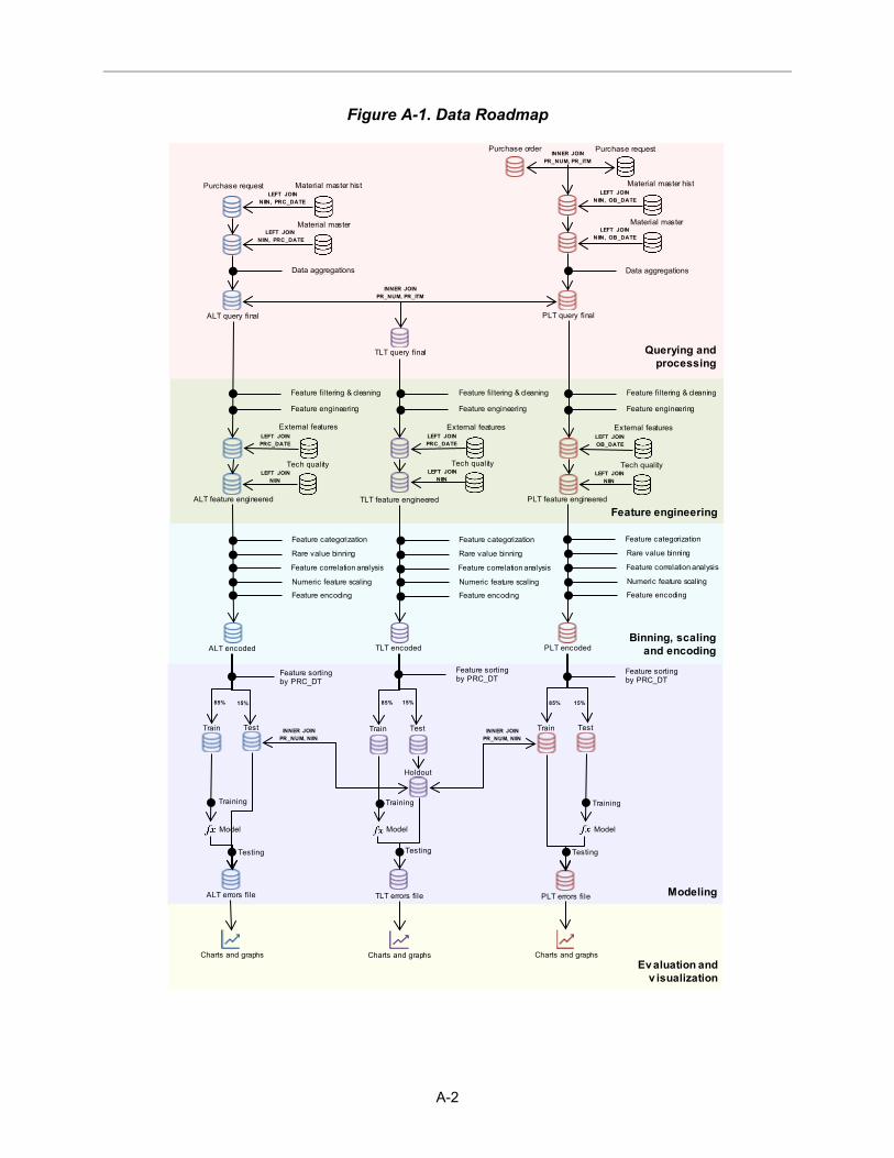
A-2

Figure A-1. Data Roadmap

Purchase order

Purchase request Material master hist

Purchase request

Material master

Data aggregations

PLT query final

Material master hist

Material master

ALT query final

INNER JOIN PR_NUM, PR_ITM

LEFT JOIN NIIN, OB_DATE

LEFT JOIN NIIN, OB_DATE

LEFT JOIN NIIN, PRC_DATE

LEFT JOIN NIIN, PRC_DATE

Data aggregations

INNER JOINPR_NUM, PR_ITM

TLT query final

Tech qualityLEFT JOIN

NIIN

LEFT JOINOB_DATE


NIIN

LEFT JOINPRC_DATE

External features


NIIN

LEFT JOINPRC_DATE

Feature filtering & cleaning

ALT feature engineered

ALT encoded

TLT feature engineered

TLT encoded

PLT feature engineered

Feature categorization

Rare value binning

Feature correlation analysis

Numeric feature scaling

Feature encoding

PLT encoded

Feature engineering

Feature sorting by PRC_DT

ALT errors file TLT errors file PLT errors file

Charts and graphsCharts and graphsCharts and graphs

Holdout

Train INNER JOINPR_NUM, NIIN


Test

Training

Testing

Training

Testing

15%

Training

Testing

Querying and processing

Feature engineering

Binning, scalingand encoding

Modeling

Ev aluation and v isualization

Train Test Train Test

External features External features



85% 15%85% 15%85%


Rare value binning



Feature encoding


Rare value binning



Feature encoding


Feature engineering


Feature engineering

Model ModelModel

B-1

Appendix B Feature Lists

The tables in this appendix contain the full list of features for each model. These features include data from DLA or external data as well as engineered features.

Table B-1. ALT Features

Feature variable Feature name Description

Engineered Features buyer_wl_prof_ctr Profit Center Workload For the NIIN’s profit center, the number of open

PRs at the time of PR creation common_awdtype Common Award Type For an NIIN, the most common award type for the

most recent award month common_class_sply Common Class of Supply For an NIIN, the most common class of supply for

the most recent award month common_doctype_re Common Doctype For an NIIN, the most common PO doctype of the

most recent award month common_doctype_setback_re Common Doctype

(10-month lookback) For an NIIN, the most common PO doctype of the 10 most recent award months

common_plant Common Plant For an NIIN, the most common plant for the most recent award month

common_prioritycd Common Priority Code For an NIIN, the most common priority code for the most recent award month

common_schain Common Supply Chain 1 For an NIIN, the most common supply chain for the most recent award month (from material master)

common_splychain Common Supply Chain 2 For an NIIN, the most common supply chain for the most recent award month (from item detail)

common_stockdvd Common Stock DVD For an NIIN, the most common stock Direct Vendor Delivery (DVD) for the most recent award month

dslp Days Since Last Procurement For an NIIN, the number of days since the last PR opened

int_prc_dt_re PR Generation Date Integer representation of the PR open date mean _alt_re Mean ALT For an NIIN, the mean observed ALT for orders of

the most recent award month mean_alt_setback_re Mean ALT (1-month lookback) For an NIIN, the mean observed ALT for orders of

the second most recent award month mean_bids_setback Mean Number of Bids

(1-month lookback) For an NIIN, the mean number of bids for the second most recent award month

mean_num_bids Mean Number of Bids For an NIIN, the mean number of bids for the most recent award month

med_alt_profit_ctr_re Median ALT by Profit Center For an NIIN’s profit center, the median ALT for orders in the most recent award month

med_altr_re Median ALTR For an NIIN, the median ALTR for orders of the most recent award month

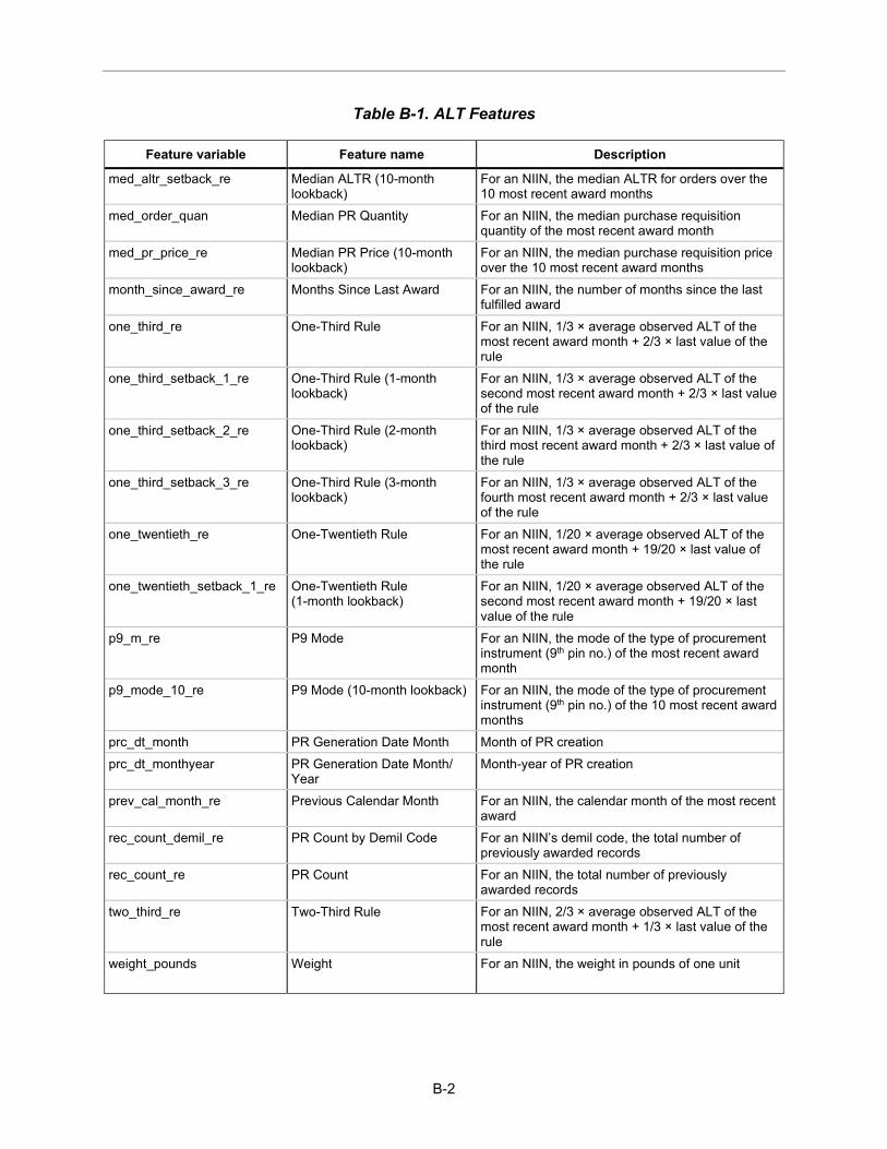
B-2



med_altr_setback_re Median ALTR (10-month lookback)

For an NIIN, the median ALTR for orders over the 10 most recent award months

med_order_quan Median PR Quantity For an NIIN, the median purchase requisition quantity of the most recent award month

med_pr_price_re Median PR Price (10-month lookback)

For an NIIN, the median purchase requisition price over the 10 most recent award months

month_since_award_re Months Since Last Award For an NIIN, the number of months since the last fulfilled award

one_third_re One-Third Rule For an NIIN, 1/3 × average observed ALT of the most recent award month + 2/3 × last value of the rule

one_third_setback_1_re One-Third Rule (1-month lookback)

For an NIIN, 1/3 × average observed ALT of the second most recent award month + 2/3 × last value of the rule


For an NIIN, 1/3 × average observed ALT of the third most recent award month + 2/3 × last value of the rule


For an NIIN, 1/3 × average observed ALT of the fourth most recent award month + 2/3 × last value of the rule

one_twentieth_re One-Twentieth Rule For an NIIN, 1/20 × average observed ALT of the most recent award month + 19/20 × last value of the rule

one_twentieth_setback_1_re One-Twentieth Rule (1-month lookback)


p9_m_re P9 Mode For an NIIN, the mode of the type of procurement instrument (9th pin no.) of the most recent award month

p9_mode_10_re P9 Mode (10-month lookback) For an NIIN, the mode of the type of procurement instrument (9th pin no.) of the 10 most recent award months

prc_dt_month PR Generation Date Month Month of PR creation prc_dt_monthyear PR Generation Date Month/

Year Month-year of PR creation

prev_cal_month_re Previous Calendar Month For an NIIN, the calendar month of the most recent award

rec_count_demil_re PR Count by Demil Code For an NIIN’s demil code, the total number of previously awarded records

rec_count_re PR Count For an NIIN, the total number of previously awarded records

two_third_re Two-Third Rule For an NIIN, 2/3 × average observed ALT of the most recent award month + 1/3 × last value of the rule

weight_pounds Weight For an NIIN, the weight in pounds of one unit

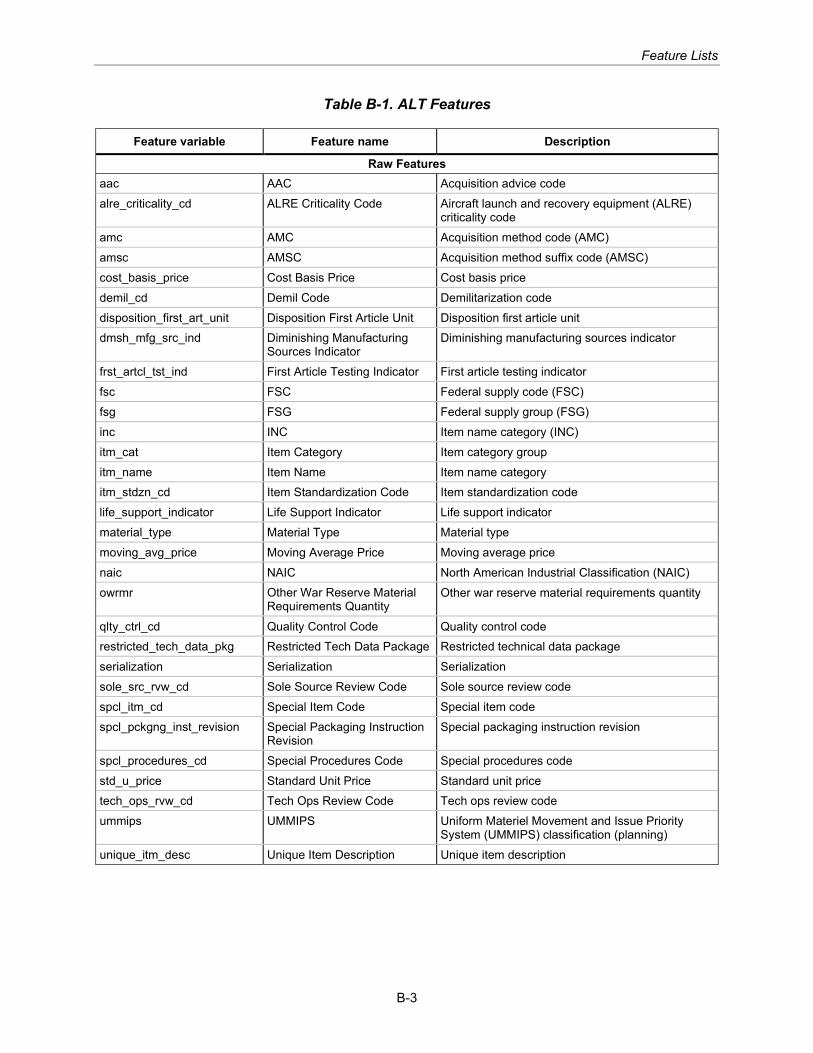
Feature Lists

B-3



Raw Features aac AAC Acquisition advice code alre_criticality_cd ALRE Criticality Code Aircraft launch and recovery equipment (ALRE)

criticality code amc AMC Acquisition method code (AMC) amsc AMSC Acquisition method suffix code (AMSC) cost_basis_price Cost Basis Price Cost basis price demil_cd Demil Code Demilitarization code disposition_first_art_unit Disposition First Article Unit Disposition first article unit dmsh_mfg_src_ind Diminishing Manufacturing

Sources Indicator Diminishing manufacturing sources indicator

frst_artcl_tst_ind First Article Testing Indicator First article testing indicator fsc FSC Federal supply code (FSC) fsg FSG Federal supply group (FSG) inc INC Item name category (INC) itm_cat Item Category Item category group itm_name Item Name Item name category itm_stdzn_cd Item Standardization Code Item standardization code life_support_indicator Life Support Indicator Life support indicator material_type Material Type Material type moving_avg_price Moving Average Price Moving average price naic NAIC North American Industrial Classification (NAIC) owrmr Other War Reserve Material

Requirements Quantity Other war reserve material requirements quantity

qlty_ctrl_cd Quality Control Code Quality control code restricted_tech_data_pkg Restricted Tech Data Package Restricted technical data package serialization Serialization Serialization sole_src_rvw_cd Sole Source Review Code Sole source review code spcl_itm_cd Special Item Code Special item code spcl_pckgng_inst_revision Special Packaging Instruction

Revision Special packaging instruction revision

spcl_procedures_cd Special Procedures Code Special procedures code std_u_price Standard Unit Price Standard unit price tech_ops_rvw_cd Tech Ops Review Code Tech ops review code ummips UMMIPS Uniform Materiel Movement and Issue Priority

System (UMMIPS) classification (planning) unique_itm_desc Unique Item Description Unique item description

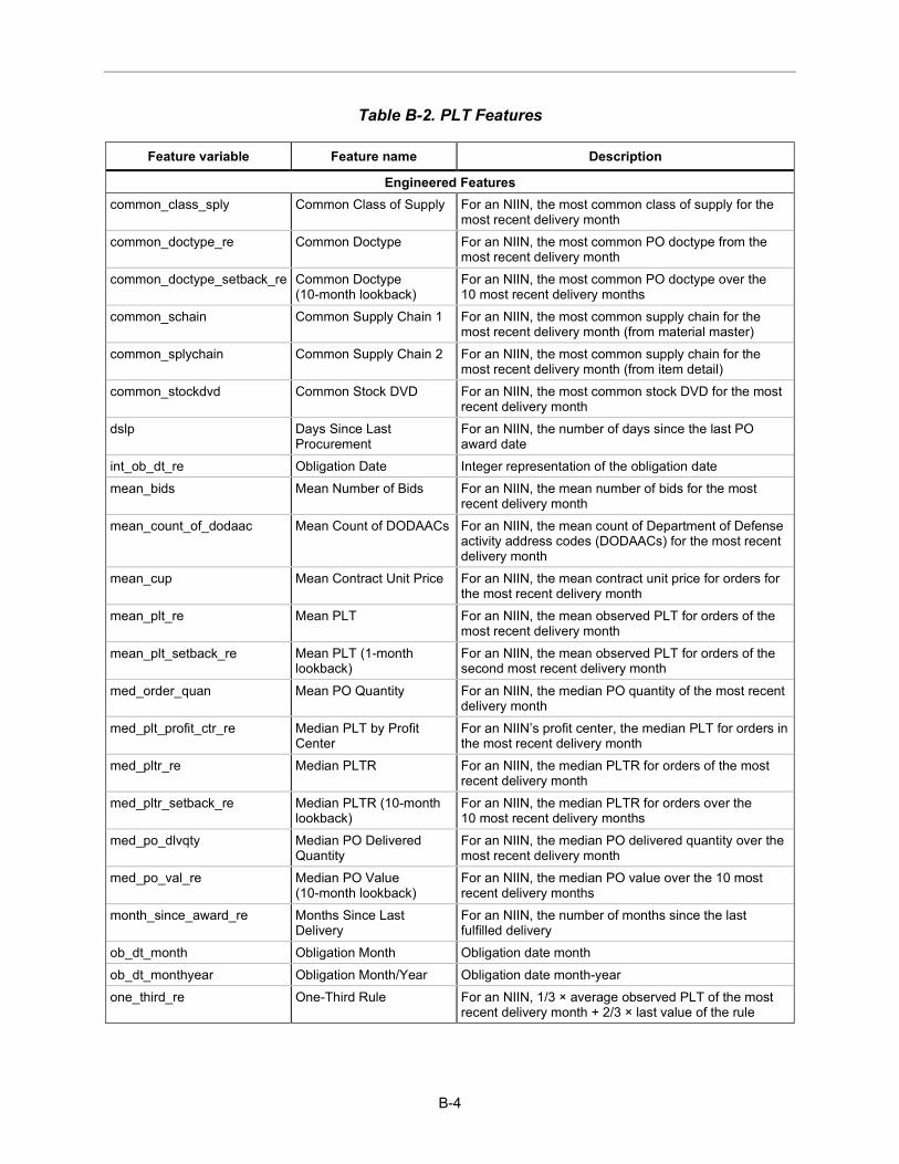
B-4

Table B-2. PLT Features


Engineered Features common_class_sply Common Class of Supply For an NIIN, the most common class of supply for the

most recent delivery month common_doctype_re Common Doctype For an NIIN, the most common PO doctype from the

most recent delivery month common_doctype_setback_re Common Doctype

(10-month lookback) For an NIIN, the most common PO doctype over the 10 most recent delivery months

common_schain Common Supply Chain 1 For an NIIN, the most common supply chain for the most recent delivery month (from material master)

common_splychain Common Supply Chain 2 For an NIIN, the most common supply chain for the most recent delivery month (from item detail)

common_stockdvd Common Stock DVD For an NIIN, the most common stock DVD for the most recent delivery month

dslp Days Since Last Procurement

For an NIIN, the number of days since the last PO award date

int_ob_dt_re Obligation Date Integer representation of the obligation date mean_bids Mean Number of Bids For an NIIN, the mean number of bids for the most

recent delivery month mean_count_of_dodaac Mean Count of DODAACs For an NIIN, the mean count of Department of Defense

activity address codes (DODAACs) for the most recent delivery month

mean_cup Mean Contract Unit Price For an NIIN, the mean contract unit price for orders for the most recent delivery month

mean_plt_re Mean PLT For an NIIN, the mean observed PLT for orders of the most recent delivery month

mean_plt_setback_re Mean PLT (1-month lookback)

For an NIIN, the mean observed PLT for orders of the second most recent delivery month

med_order_quan Mean PO Quantity For an NIIN, the median PO quantity of the most recent delivery month

med_plt_profit_ctr_re Median PLT by Profit Center

For an NIIN’s profit center, the median PLT for orders in the most recent delivery month

med_pltr_re Median PLTR For an NIIN, the median PLTR for orders of the most recent delivery month

med_pltr_setback_re Median PLTR (10-month lookback)

For an NIIN, the median PLTR for orders over the 10 most recent delivery months

med_po_dlvqty Median PO Delivered Quantity

For an NIIN, the median PO delivered quantity over the most recent delivery month

med_po_val_re Median PO Value (10-month lookback)

For an NIIN, the median PO value over the 10 most recent delivery months

month_since_award_re Months Since Last Delivery

For an NIIN, the number of months since the last fulfilled delivery

ob_dt_month Obligation Month Obligation date month ob_dt_monthyear Obligation Month/Year Obligation date month-year one_third_re One-Third Rule For an NIIN, 1/3 × average observed PLT of the most

recent delivery month + 2/3 × last value of the rule

Feature Lists

B-5




For an NIIN, 1/3 × average observed PLT of the second most recent delivery month + 2/3 × last value of the rule


For an NIIN, 1/3 × average observed PLT of the third most recent delivery month + 2/3 × last value of the rule


For an NIIN, 1/3 × average observed PLT of the fourth most recent delivery month + 2/3 × last value of the rule

one_twentieth_re One-Twentieth Rule For an NIIN, 1/20 × average observed PLT of the most recent delivery month + 19/20 × last value of the rule


For an NIIN, 1/20 × average observed PLT of the second most recent delivery month + 19/20 × last value of the rule

p9_m_re P9 Mode For an NIIN, the mode of the type of procurement instrument (9th pin no.) of the most recent delivery month

p9_mode_10_re P9 Mode (10-month lookback)

For an NIIN, the mode of the type of procurement instrument (9th pin no.) of the 10 most recent delivery months

prev_cal_month_re Previous Calendar Month For an NIIN, the calendar month of the most recent delivery

rec_count_demil_re PO Count by demil code For an NIIN’s demil code, the total number of previously awarded records

rec_count_re PO Count For an NIIN, the total number of previously awarded records

two_third_re Two-Third Rule For an NIIN, 2/3 × average observed PLT of the most recent delivery month + 1/3 × last value of the rule

weight_pounds Weight For an NIIN, the weight in pounds of one unit Raw Features

aac AAC AAC alre_criticality_cd ALRE Criticality Code ALRE criticality code amc AMC AMC amsc AMSC AMSC cost_basis_price Cost Basis Price Cost basis price demil_cd Demilitarization Code Demilitarization code disposition_first_art_unit Disposition First Art Unit Disposition first art unit dmsh_mfg_src_ind Diminishing Manufacturing

Sources Indicator Diminishing manufacturing sources indicator

doctype Purchasing Document Type Purchasing document type ext_aircraft PPI Aircraft

Manufacturing: General Producer price index (PPI) by industry: aircraft manufacturing

ext_aircraftEngine PPI Aircraft Manufacturing: Engine

PPI by industry: aircraft engine and parts manufacturing: aircraft engine parts

ext_aircraftOther PPI Aircraft Manufacturing: Other Parts

PPI by industry: aircraft engine and parts manufacturing: aircraft other parts

ext_ds_equip Industrial Production: Defense and Space Equipment

Industrial production: defense and space equipment

B-6



ext_FDEFX National Defense Consumption Expenditures and Gross Investment

National defense consumption expenditures and gross investment

ext_hardware Producer Price Index by Industry: Hardware Manufacturing

Producer price index by industry: hardware manufacturing

ext_ironsteel Producer Price Index by Industry: Metals and Metal Products: Iron and Steel

Producer price index by industry: metals and metal products: iron and steel

frst_artcl_tst_ind First Article Testing Indicator

First article testing indicator

fsc Federal Supply Code FSC fsg Federal Supply Group FSG inc Item Name Category INC itm_cat_group Item Category Group Item category group itm_name Item Name Category INC itm_stdzn_cd Item Standardization Code Item standardization code life_support_indicator Life Support Indicator Life support indicator material_type Material Type Material type moving_avg_price Moving Average Price Moving average price naic North American Industrial

Classification NAIC

owrmr Other War Reserve Material Requirements Qty

Other war reserve material requirements quantity

profit_ctr Profit Center Profit center qlty_ctrl_cd Quality Control Code Quality control code restricted_tech_data_pkg Restricted Technical Data

Package Restricted technical data package

serialization Serialization Serialization sole_src_rvw_cd Sole Source Review Code Sole source review code spcl_itm_cd Special Item Code Special item code spcl_pckgng_inst_revision Special Packaging

Instruction Revision Special packaging instruction revision

spcl_procedures_cd Special Procedures Code Special procedures code std_u_price Standard Unit Price Standard unit price tech_ops_rvw_cd Tech Ops Review Code Tech ops review code total_po_val Total PO Value Total PO value total_quan Total Quantity by PO

Number and NIIN Total quantity by PO number and NIIN

ummips UMMIPS Classification (Planning)

UMMIPS classification (planning)

unique_itm_desc Unique Item Description Unique item description

Feature Lists

B-7

Table B-3. TLT Features


Engineered Features buyer_wl_prof_ctr Profit Center Workload For the NIIN’s profit center, the number of open PRs at

the time of PR creation common_awdtype Common Award Type For an NIIN, the most common award type for the most

recent award month common_class_sply Common Class of Supply For an NIIN, the most common class of supply for the

most recent award month common_doctype_re Common Doctype For an NIIN, the most common PO doctype of the most

recent award month common_doctype_setback_re Common Doctype

(10-month lookback) For an NIIN, the most common PO doctype of the 10 most recent award months

common_plant Common Plant For an NIIN, the most common plant for the most recent award month

common_prioritycd Common Priority Code For an NIIN, the most common priority code for the most recent award month

common_schain Common Supply Chain 1 For an NIIN, the most common supply chain for the most recent award month (from material master)

common_splychain Common Supply Chain 2 For an NIIN, the most common supply chain for the most recent award month (from item detail)

common_stockdvd Common Stock DVD For an NIIN, the most common stock DVD for the most recent award month

dslp Days Since Last Procurement

For an NIIN, the number of days since the last PR opened

int_prc_dt_re PR Generation Date Integer representation of the PR open date mean_alt_re Mean ALT For an NIIN, the mean observed ALT for orders of the

most recent award month mean_alt_setback_re Mean ALT (1-month

lookback) For an NIIN, the mean observed ALT for orders of the second most recent award month

mean_bids_setback Mean Number of Bids (1-month lookback)

For an NIIN, the mean number of bids for the second most recent award month

mean_num_bids Mean Number of Bids For an NIIN, the mean number of bids for the most recent award month

med_alt_profit_ctr_re Median ALT by Profit Center

For an NIIN’s profit center, the median ALT for orders in the most recent award month

med_altr_re Median ALTR For an NIIN, the median ALTR for orders of the most recent award month

med_altr_setback_re Median ALTR (10-month lookback)

For an NIIN, the median ALTR for orders over the 10 most recent award months

med_order_quan Median PR Quantity For an NIIN, the median purchase requisition quantity of the most recent award month

med_pr_price_re Median PR Price (10-month lookback)

For an NIIN, the median purchase requisition price over the 10 most recent award months

month_since_award_re Months Since Last Award For an NIIN, the number of months since the last fulfilled award

one_third_re One-Third Rule For an NIIN, 1/3 × average observed ALT of the most recent award month + 2/3 × last value of the rule

B-8






For an NIIN, 1/3 × average observed ALT of the third most recent award month + 2/3 × last value of the rule


For an NIIN, 1/3 × average observed ALT of the fourth most recent award month + 2/3 × last value of the rule

one_twentieth_re One-Twentieth Rule For an NIIN, 1/20 × average observed ALT of the most recent award month + 19/20 × last value of the rule



p9_m_re P9 Mode For an NIIN, the mode of the type of procurement instrument (9th pin no.) of the most recent award month

p9_mode_10_re P9 Mode (10-month lookback)

For an NIIN, the mode of the type of procurement instrument (9th pin no.) of the 10 most recent award months

prc_dt_month PR Generation Date Month Month of PR creation prc_dt_monthyear PR Generation Date

Month/Year Month-year of PR creation

prev_cal_month_re Previous Calendar Month For an NIIN, the calendar month of the most recent award

rec_count_demil_re PR Count by Demil Code For an NIIN’s demil code, the total number of previously awarded records

rec_count_re PR Count For an NIIN, the total number of previously awarded records

two_third_re Two-Third Rule For an NIIN, 2/3 × average observed ALT of the most recent award month + 1/3 × last value of the rule

weight_pounds Weight For an NIIN, the weight in pounds of one unit Raw Features

aac AAC AAC alre_criticality_cd alre_criticality_cd ALRE criticality code amc AMC AMC amsc AMSC AMSC cost_basis_price cost_basis_price Cost basis price demil_cd Demil Code Demilitarization code disposition_first_art_unit disposition_first_art_unit Disposition first art unit dmsh_mfg_src_ind dmsh_mfg_src_ind Diminishing manufacturing sources indicator frst_artcl_tst_ind frst_artcl_tst_ind First article testing indicator fsc FSC Federal supply code fsg FSG Federal supply group inc INC INC itm_cat Item Category Item category group itm_name Item Name INC itm_stdzn_cd itm_stdzn_cd Item standardization code

Feature Lists

B-9



life_support_indicator life_support_indicator Life support indicator material_type material_type Material type moving_avg_price moving_avg_price Moving average price naic NAIC NAIC owrmr owrmr Other war reserve material requirements quantity qlty_ctrl_cd qlty_ctrl_cd Quality control code restricted_tech_data_pkg restricted_tech_data_pkg Restricted technical data package serialization serialization Serialization sole_src_rvw_cd sole_src_rvw_cd Sole source review code spcl_itm_cd spcl_itm_cd Special item code spcl_pckgng_inst_revision spcl_pckgng_inst_revision Special packaging instruction revision spcl_procedures_cd spcl_procedures_cd Special procedures code std_u_price Standard Unit Price Standard unit price tech_ops_rvw_cd tech_ops_rvw_cd Tech ops review code ummips UMMIPS UMMIPS classification (planning) unique_itm_desc unique_itm_desc Unique item description

C-1

Appendix C Aggregation Rules

Prior to any modelling, the data needs to be modified so PR-NIIN (ALT dataset), PO-NIIN (PLT dataset), or PR-PO-NIIN (TLT dataset) functions as a unique ID for each dataset. Aggregation rules are used to consolidate records with the same unique ID. Unrelated aggregation methods are used to engineer new features, which are described in Historical Aggregations of Raw Features section of Chapter 2.

First, numeric columns involving quantity, price, or value are summed for a single total quantity, price, or value column per PO-NIIN, PR-NIIN, or PR-PO-NIIN. Any other numeric columns are aggregated by taking the mean of the different unique values, while categorical columns are aggregated by taking the earliest or the latest unique value based on date. If the column is from the PO or PR tables, the earliest value represents the information known at the moment of procurement or obligation; if the column is from the NIIN-level tables, such as material master or item detail, the last value represents the most up-to-date values of that NIIN.

Although a raw column may be in both the PLT and ALT modeling datasets, the column may not need aggregation in both. For example, MOVING_AVG_PRICE exists in both ALT and PLT modeling datasets, but is not aggregated at the PO-NIIN level as each PO-NIIN had one MOVING_AVG_PRICE value—different from the PR-NIIN level. Table C-1 defines the data aggregation rues applied to the ALT data.

Table C-1. ALT Data Aggregation Rules

Aggregated column Raw column Aggregate function

Actual Procurement Date (act_prcrt_dt) ACTPRCRTDT First Award Type (awd_type) AWD_TYPE First Buyer ID (buyr_id) BUYR_ID First CAGE ID (cage_id) CAGE_ID First Delivery (delivery) DELIVERY Last Document Date (doc_date) DOC_DATE First Federal Supply Code (fsc) FSC Last Item Category (item_cat) ITM_CAT First Last Change Date (last_chgdt) LAST_CHGDT Last Mean ALTR (mean_altr) ALTR Mean Mean Contract Unit Price (mean_cup) CUP Mean Mean Cost Basis Price (mean_cost_basis_price) COST_BASIS_PRICE Mean Mean Moving Average Price (mean_moving_avg_price) MOVING_AVG_PRICE Mean Mean PLTR (mean_pltr) PLTR Mean Mean Standard Unit Price (mean_std_u_price_hist) STD_U_PRICE_HIST Mean

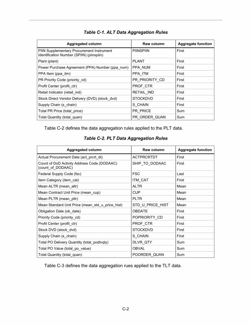
C-2

Table C-1. ALT Data Aggregation Rules


PIIN Supplementary Procurement Instrument Identification Number (SPIIN) (piinspiin)

PIINSPIIN First

Plant (plant) PLANT First Power Purchase Agreement (PPA) Number (ppa_num) PPA_NUM First PPA Item (ppa_itm) PPA_ITM First PR Priority Code (priority_cd) PR_PRIORITY_CD First Profit Center (profit_ctr) PROF_CTR First Retail Indicator (retail_ind) RETAIL_IND First Stock Direct Vendor Delivery (DVD) (stock_dvd) STOCKDVD First Supply Chain (s_chain) S_CHAIN First Total PR Price (total_price) PR_PRICE Sum Total Quantity (total_quan) PR_ORDER_QUAN Sum

Table C-2 defines the data aggregation rules applied to the PLT data.

Table C-2. PLT Data Aggregation Rules


Actual Procurement Date (act_prcrt_dt) ACTPRCRTDT First Count of DoD Activity Address Code (DODAAC) (count_of_DODAAC)

SHIP_TO_DODAAC First

Federal Supply Code (fsc) FSC Last Item Category (item_cat) ITM_CAT First Mean ALTR (mean_altr) ALTR Mean Mean Contract Unit Price (mean_cup) CUP Mean Mean PLTR (mean_pltr) PLTR Mean Mean Standard Unit Price (mean_std_u_price_hist) STD_U_PRICE_HIST Mean Obligation Date (ob_date) OBDATE First Priority Code (priority_cd) POPRIORITY_CD First Profit Center (profit_ctr) PROF_CTR First Stock DVD (stock_dvd) STOCKDVD First Supply Chain (s_chain) S_CHAIN First Total PO Delivery Quantity (total_podlvqty) DLVR_QTY Sum Total PO Value (total_po_value) OBVAL Sum Total Quantity (total_quan) POORDER_QUAN Sum

Table C-3 defines the data aggregation rues applied to the TLT data.

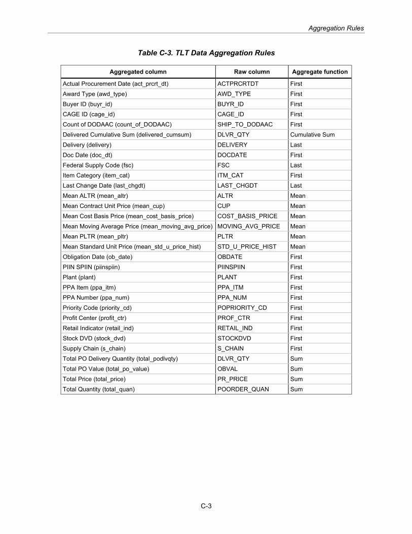
Aggregation Rules

C-3

Table C-3. TLT Data Aggregation Rules


Actual Procurement Date (act_prcrt_dt) ACTPRCRTDT First Award Type (awd_type) AWD_TYPE First Buyer ID (buyr_id) BUYR_ID First CAGE ID (cage_id) CAGE_ID First Count of DODAAC (count_of_DODAAC) SHIP_TO_DODAAC First Delivered Cumulative Sum (delivered_cumsum) DLVR_QTY Cumulative Sum Delivery (delivery) DELIVERY Last Doc Date (doc_dt) DOCDATE First Federal Supply Code (fsc) FSC Last Item Category (item_cat) ITM_CAT First Last Change Date (last_chgdt) LAST_CHGDT Last Mean ALTR (mean_altr) ALTR Mean Mean Contract Unit Price (mean_cup) CUP Mean Mean Cost Basis Price (mean_cost_basis_price) COST_BASIS_PRICE Mean Mean Moving Average Price (mean_moving_avg_price) MOVING_AVG_PRICE Mean Mean PLTR (mean_pltr) PLTR Mean Mean Standard Unit Price (mean_std_u_price_hist) STD_U_PRICE_HIST Mean Obligation Date (ob_date) OBDATE First PIIN SPIIN (piinspiin) PIINSPIIN First Plant (plant) PLANT First PPA Item (ppa_itm) PPA_ITM First PPA Number (ppa_num) PPA_NUM First Priority Code (priority_cd) POPRIORITY_CD First Profit Center (profit_ctr) PROF_CTR First Retail Indicator (retail_ind) RETAIL_IND First Stock DVD (stock_dvd) STOCKDVD First Supply Chain (s_chain) S_CHAIN First Total PO Delivery Quantity (total_podlvqty) DLVR_QTY Sum Total PO Value (total_po_value) OBVAL Sum Total Price (total_price) PR_PRICE Sum Total Quantity (total_quan) POORDER_QUAN Sum

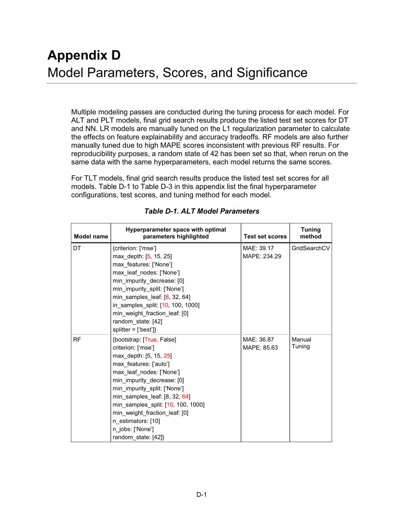
D-1

Appendix D Model Parameters, Scores, and Significance

Multiple modeling passes are conducted during the tuning process for each model. For ALT and PLT models, final grid search results produce the listed test set scores for DT and NN. LR models are manually tuned on the L1 regularization parameter to calculate the effects on feature explainability and accuracy tradeoffs. RF models are also further manually tuned due to high MAPE scores inconsistent with previous RF results. For reproducibility purposes, a random state of 42 has been set so that, when rerun on the same data with the same hyperparameters, each model returns the same scores.

For TLT models, final grid search results produce the listed test set scores for all models. Table D-1 to Table D-3 in this appendix list the final hyperparameter configurations, test scores, and tuning method for each model.

Table D-1. ALT Model Parameters

Model name Hyperparameter space with optimal

parameters highlighted Test set scores Tuning method

DT {criterion: [‘mse’] max_depth: [5, 15, 25] max_features: [‘None’] max_leaf_nodes: [‘None’] min_impurity_decrease: [0] min_impurity_split: [‘None’] min_samples_leaf: [8, 32, 64] in_samples_split: [10, 100, 1000] min_weight_fraction_leaf: [0] random_state: [42] splitter = [‘best’]}

MAE: 39.17 MAPE: 234.29

GridSearchCV

RF {bootstrap: [True, False] criterion: [‘mse’] max_depth: [5, 15, 25] max_features: [‘auto’] max_leaf_nodes: [‘None’] min_impurity_decrease: [0] min_impurity_split: [‘None’] min_samples_leaf: [8, 32, 64] min_samples_split: [10, 100, 1000] min_weight_fraction_leaf: [0] n_estimators: [10] n_jobs: [‘None’] random_state: [42]}

MAE: 36.87 MAPE: 85.63

Manual Tuning

D-2

Table D-1. ALT Model Parameters

Model name Hyperparameter space with optimal

parameters highlighted Test set scores Tuning method

LR {alpha: [0.0001, 0.001, 0.01] average: [False] early_stopping: [False] epsilon: [0.1] eta: [0.01] fit_intercept: [True] l1_ratio: [0.15] learning_rate: [‘invscaling’] loss: [‘huber’, ‘squared_loss’] max_iter: [‘None’] n_iter: [‘None’] n_iter_no_change: [5] penalty: [‘l1’,’l2’,’elasticNet’, ‘None’] power_t: [0.25] random_state: [42] shuffle: [True] validation_fraction: [0.1] warm_start: [False]}

MAE: 37.84 MAPE: 135.80

Manual Tuning

NN {activation: [‘tanh’, ‘relu’] alpha: [0.0001] batch_size: [auto] beta_1: [0.9] beta_2: [.99] early_stopping: [False] epsilon: [1e-08] hidden_layer_size: [(10,), (25, 5), (50,), (50, 25)] learning_rate: [‘constant’, ‘invscaling’, ‘adaptive’] learning_rate_init: [0.1, 0.01, 0.001] max_iter: [200] momentum: [0.9] n_iter_no_change: [10] nesterovs_momentum: True power_t: [0.5] random_state: [42] shuffle: [True] solver: [‘adam’] tol: [0.0001] validation_fraction: [0.1] warm_start: [False]}

MAE: 41.74 MAPE: 280.45

GridSearchCV

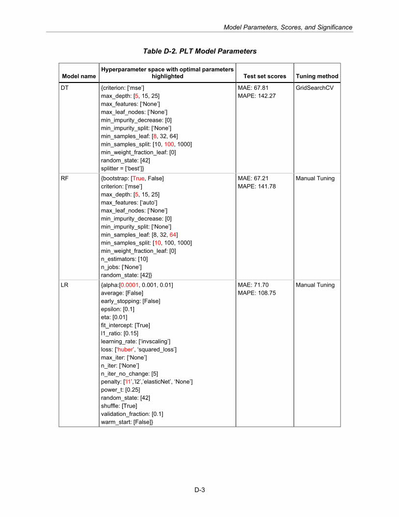
Model Parameters, Scores, and Significance

D-3

Table D-2. PLT Model Parameters

Model name Hyperparameter space with optimal parameters

highlighted Test set scores Tuning method

DT {criterion: [‘mse’] max_depth: [5, 15, 25] max_features: [‘None’] max_leaf_nodes: [‘None’] min_impurity_decrease: [0] min_impurity_split: [‘None’] min_samples_leaf: [8, 32, 64] min_samples_split: [10, 100, 1000] min_weight_fraction_leaf: [0] random_state: [42] splitter = [‘best’]}

MAE: 67.81 MAPE: 142.27

GridSearchCV

RF {bootstrap: [True, False] criterion: [‘mse’] max_depth: [5, 15, 25] max_features: [‘auto’] max_leaf_nodes: [‘None’] min_impurity_decrease: [0] min_impurity_split: [‘None’] min_samples_leaf: [8, 32, 64] min_samples_split: [10, 100, 1000] min_weight_fraction_leaf: [0] n_estimators: [10] n_jobs: [‘None’] random_state: [42]}

MAE: 67.21 MAPE: 141.78

Manual Tuning

LR {alpha:[0.0001, 0.001, 0.01] average: [False] early_stopping: [False] epsilon: [0.1] eta: [0.01] fit_intercept: [True] l1_ratio: [0.15] learning_rate: [‘invscaling’] loss: [‘huber’, ‘squared_loss’] max_iter: [‘None’] n_iter: [‘None’] n_iter_no_change: [5] penalty: [‘l1’,’l2’,’elasticNet’, ‘None’] power_t: [0.25] random_state: [42] shuffle: [True] validation_fraction: [0.1] warm_start: [False]}

MAE: 71.70 MAPE: 108.75

Manual Tuning

D-4

Table D-2. PLT Model Parameters

Model name Hyperparameter space with optimal parameters

highlighted Test set scores Tuning method

NN {activation: [‘tanh’, ‘relu’] alpha: [0.0001] batch_size: [auto] beta_1: [0.9] beta_2: [.99] early_stopping: [False] epsilon: [1e-08] hidden_layer_size: [(10,), (25, 5), (50,), (50, 25)] learning_rate: [‘constant’, ‘invscaling’, ‘adaptive’] learning_rate_init: [0.1, 0.01, 0.001] max_iter: [200] momentum: [0.9] n_iter_no_change: [10] nesterovs_momentum: [True] power_t: [0.5] random_state: [42] shuffle: [True] solver: [‘adam’] tol: [0.0001] validation_fraction: [0.1] warm_start: [False]}

MAE: 71.66 MAPE: 153.57

GridSearchCV

Table D-3. TLT Model Parameters

Model name Hypermeter space with optimal parameters

highlighted Holdout set scores Tuning method

Unified RF {bootstrap: [True, False] criterion: [‘mse’] max_depth: [5, 15, 25] max_features: [‘auto’] max_leaf_nodes: [‘None’] min_impurity_decrease: [0] min_impurity_split: [‘None’] min_samples_leaf: [8, 32, 64] min_samples_split: [10, 100, 1000] min_weight_fraction_leaf: [0] n_estimators: [10] n_jobs: [‘None’] random_state: [‘None’]}

MAE: 69.98 MAPE: 61.66

GridSearchCV

Model Parameters, Scores, and Significance

D-5

Table D-3. TLT Model Parameters

Model name Hypermeter space with optimal parameters

highlighted Holdout set scores Tuning method

Unified LR {alpha: [0.0001, 0.001, 0.01] average: [False] early_stopping: [False] epsilon: [0.1] eta: [0.01] fit_intercept: [True] l1_ratio: [0.15] learning_rate: [‘invscaling’] loss: [‘huber’, ‘squared_loss’] max_iter: [‘None’] n_iter: [‘None’] n_iter_no_change: [5] penalty: [‘l1’,’l2’,’elasticNet’, ‘None’] power_t: [0.25] random_state: [42] shuffle: [True] validation_fraction: [0.1] warm_start: [False]}

MAE: 62.04 MAPE: 77.12

GridSearchCV

Unified NN {activation: [‘tanh’, ‘relu’] alpha: [0.0001, 0.001, 0.01] batch_size: [auto] beta_1: [0.9] beta_2: [.99] early_stopping: [False] epsilon: [1e-08] hidden_layer_size: [(10,), (25, 5), (50)] learning_rate: [‘constant’, ‘invscaling’, ‘adaptive’] learning_rate_init: [0.1] max_iter: [150] momentum: [0.9] n_iter_no_change: [10] nesterovs_momentum: True power_t: [0.5] random_state: [None] shuffle: [True] solver: [‘adam’] tol: [0.001] validation_fraction: [0.1]}

MAE: 67.05 MAPE: 106.25

GridSearchCV

Composite RF

See ALT and PLT RF Grids MAE: 56.39 MAPE: 75.37

See ALT and PLT RF Grids

Composite LR See ALT and PLT LR Grids MAE: 62.02 MAPE: 70.53

See ALT and PLT LR Grids

RF and LR perform best based on our evaluation metrics through the initial modeling passes. From there, hyperparameters are further tuned to get the best modeling results while considering model simplicity and effect on over- or underestimates. RF ultimately performs best; therefore, we conducted Welch’s t-tests (see Table D-4 and Table D-5)

D-6

between the RF errors and each of the baselines/LR errors to check whether differences in MAE and MAPE across them are statistically significant (i.e., that the lower mean errors for RF are not purely chance). Since all p-values are 0, we conclude that the mean absolute and percent error for the RF models are smaller than each of the compared models.

Table D-4. ALT Random Forest T-Tests

Model errors compared against Type of error T-statistic P-value

ALTR Absolute Error −320 0 ALT One-Third Rule Absolute Error −311 0 ALT LR Absolute Error −30 0 ALTR Percent Error −293 0 ALT One-Third Rule Percent Error −279 0 ALT LR Percent Error −93 0

Table D-5. PLT Random Forest T-Tests

Model errors compared against Type of error T-statistic P-value

PLTR Absolute Error −114 0 PLT One-Third Rule Absolute Error −74 0 PLT LR Absolute Error −87 0 PLTR Percent Error −90 0 PLT One-Third Rule Percent Error −67 0 PLT LR Percent Error 70 0

E-1

Appendix E ML Regression Model Descriptions

Regression is a statistical measure for calculating the correlation between a selected dependent variable (the target) and a set of independent variables (the features). In a regression problem, the dependent variable is continuous, rather than discrete. Since observed lead time variables are measured in days, they are continuous. Various ML algorithms can be applied to regression problems; the four approaches for lead time estimation that we evaluated in this report are described below.

Decision Tree DT is a ML model that predict the target by learning decision rules derived from features in data. Modeled as tree-like graphs, a DT is comprised of nodes (a feature condition), branches (a value or threshold of that feature), and leaves (a predicted output). The general algorithm for DT picks the optimal feature for each node (based on how precisely the feature can split the data on its target) during training, and then traverses the DT to classify datapoints during testing and inference. DTs are interpretable because they are visualized easily, explainable because they indicate feature importance, and robust because they capture certain nonlinear relationships in the data; however, they are liable to overfitting if not explicitly corrected, and prone to instability after small changes to the input data.

Feature importance for tree models (like DT and RF), is calculated as the decrease in node impurity weighted by the node probability (the likelihood of reaching that node). A tree model consists of many nodes that apply filters (e.g., Is the median purchase order value greater than 50?) that lead to a final leaf node with a predicted value. Node impurity measures the decrease in MSE for that node. A feature may be part of multiple nodes, so a feature’s node impurity is aggregated. Node probability is the number of samples that reach the node divided by the total number of samples.

E-2

Random Forest RF is an ensemble method that is comprised of multiple uncorrelated DTs formed by randomly sampling the training set and fitting individual trees to each random set. RFs make predictions on data by applying all component decisions trees to an observation and calculating the average of predicted values. RFs are interpretable and robust for the same reason DTs are and are less liable to overfitting. They are ineffective for non-stationary data and have a higher computational cost and are less explainable than DTs due to being ensemble methods.

Linear Regression LR is a statistical modeling method, uses a linear equation to model the relationship between a set of features (independent variables) and a target (dependent variable). LR methods find optimal coefficients values for each term in the linear equation by using the least squares method, minimizing the sum of the squared distances between each datapoint and the line. To account for possible overfitting, regularization techniques add penalties to the loss function, resulting in the regularized least absolute shrinkage and selection operator (LASSO) and ridge regression variants of LR. LASSO regression allows coefficient values to reach absolute zero, thus enabling feature selection. Regularized LR models are simple to implement, interpret, and explain; they are also less likely to overfit. However, they cannot capture nonlinear relationships in the data.

ML Regression Model Descriptions

E-3

Neural Network NNs are biologically inspired computation networks comprised of simple, interconnected nodes that process an input vector of feature values into a desired output vector of the target. Neural networks include processing nodes (neurons), weighted edges between neurons (synapses), and layers (structured collections of neurons). NN training involves forward propagation algorithms (which propagate input vectors through the network and return an output vector) and back propagation algorithms (which adjust edge weights in the network using minimization and partial differentiation), enabling NNs to approximate linear and nonlinear functions. NNs are best for capturing data with nonlinearities and are often more accurate than other models for problems with large amounts of data; however, they are hard to interpret and explain. NNs are more computationally expensive than most other models.

F-1

Appendix F Model Metrics

Metric Categories The modeling and evaluation process uses three categories of metrics.

Model optimization with loss functions: Given a model and a set of labeled data, a loss function describes the difference between the model’s label predictions and the true label values. The loss function for a model is minimized during model training and optimization. Two loss functions (MSE and Huber) are implemented and defined in the Metrics Definitions section.

Hyperparameter tuning with scoring metrics: Hyperparameters are model parameters whose values must be manually set prior to model training. During cross-validation, a scoring metric for a model type compares an array of validation set scores for different hyperparameter configurations of the model. One scoring metric (MAE) is implemented and defined in the Metrics Definitions section.

Model selection and comparison with evaluation metrics: Evaluation metrics compare AI models with each other as well as against baseline methods. Two evaluation metrics (MAE and MAPE) are implemented and defined in the Metrics Definitions section.

Metric Definitions Mean Absolute Error

ℒ (𝑄𝑄,𝑄𝑄�) = ∑ |𝑄𝑄�𝑖𝑖 − 𝑄𝑄𝑖𝑖|𝑛𝑛𝑖𝑖=1

𝑚𝑚

The average of the sum of absolute differences between a model’s predicted values and the true target values, MAE measures a model’s raw error by averaging the absolute errors, where 𝑄𝑄𝑖𝑖 is the true observed value, 𝑄𝑄�𝑖𝑖 is the predicted value, and 𝑚𝑚 is the number of observations in the dataset.

While the primary evaluation metric for all models, MAE is not available as a loss function for LR and NN (since MAE is a nondifferentiable loss function, it cannot be used for linear and neural models optimized on stochastic gradient descent). For tree models, MAE is an available loss function, but unused due to known computation and memory limitations. During the validation process, MAE is the scoring metric for all grid searches. After modeling, MAE is a primary evaluation metric when comparing model outputs.

F-2

Mean Squared Error

ℒ (𝑄𝑄,𝑄𝑄�) =∑ (𝑄𝑄�𝑖𝑖 − 𝑄𝑄𝑖𝑖)2𝑛𝑛𝑖𝑖=1

𝑚𝑚

The average of the sum of squared differences (squared loss) between a model’s predicted values and the true target values, MSE measures the standard deviation of a model’s errors, where 𝑄𝑄�𝑖𝑖 is the predicted value, 𝑄𝑄𝑖𝑖 is the true observed value, and 𝑚𝑚 is the number of observations in the dataset.

MSE is the selected loss function for both tree models. Squared loss (MSE without averaging to a single value) is also used as the loss function for the NN model and an assessed loss function for LR.

Huber

ℒ (𝑄𝑄,𝑄𝑄�) = � 12

(𝑄𝑄�𝑖𝑖 − 𝑄𝑄𝑖𝑖)2 (𝑄𝑄�𝑖𝑖 − 𝑄𝑄𝑖𝑖) < 𝜀𝜀

𝜀𝜀 |(𝑄𝑄�𝑖𝑖 − 𝑄𝑄𝑖𝑖)|–12𝜀𝜀2 (𝑄𝑄�𝑖𝑖 − 𝑄𝑄𝑖𝑖) > 𝜀𝜀

A piecewise loss function composed of absolute loss and squared loss variants, Huber combines the outlier robustness found in absolute loss for larger errors with the differentiability of squared loss for smaller errors. 𝑄𝑄�𝑖𝑖 is the predicted value, 𝑄𝑄𝑖𝑖 is the true observed value, and 𝑚𝑚 is the number of observations in the dataset. 𝜀𝜀 is the error threshold for switching between absolute and squared loss variants.

Huber is the selected loss function for LR.

Mean Absolute Percentage Error

ℒ (𝑄𝑄,𝑄𝑄�) =

∑ |𝑄𝑄�𝑖𝑖 − 𝑄𝑄𝑖𝑖|𝑛𝑛𝑖𝑖=1

𝑄𝑄𝑖𝑖𝑚𝑚

𝐸𝐸 100

The average of the absolute percentage errors, MAPE measures a model’s magnitude of error, where 𝑄𝑄𝑖𝑖 is the true observed value, 𝑄𝑄�𝑖𝑖 is the predicted value, and 𝑚𝑚 is the number of observations in the dataset.

A divide-by-zero problem can occur with MAPE if 𝑄𝑄𝑖𝑖 = 0, so the dataset is filtered to exclude all rows where observed ALT or observed PLT are equal to 0. After modeling, MAPE is a secondary evaluation metric when comparing model outputs.

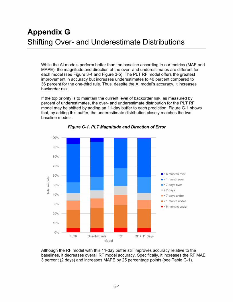
G-1

Appendix G Shifting Over- and Underestimate Distributions

While the AI models perform better than the baseline according to our metrics (MAE and MAPE), the magnitude and direction of the over- and underestimates are different for each model (see Figure 3-4 and Figure 3-5). The PLT RF model offers the greatest improvement in accuracy but increases underestimates to 40 percent compared to 36 percent for the one-third rule. Thus, despite the AI model’s accuracy, it increases backorder risk.

If the top priority is to maintain the current level of backorder risk, as measured by percent of underestimates, the over- and underestimate distribution for the PLT RF model may be shifted by adding an 11-day buffer to each prediction. Figure G-1 shows that, by adding this buffer, the underestimate distribution closely matches the two baseline models.

Figure G-1. PLT Magnitude and Direction of Error

Although the RF model with this 11-day buffer still improves accuracy relative to the baselines, it decreases overall RF model accuracy. Specifically, it increases the RF MAE 3 percent (2 days) and increases MAPE by 25 percentage points (see Table G-1).

0%

10%

20%

30%

40%

50%

60%

70%

80%

90%

100%

PLTR One-third rule RF RF + 11 Days

Tota

l rec

ords

Model

> 6 months over

> 1 month over

> 7 days over

± 7 days

> 7 days under

> 1 month under

> 6 months under

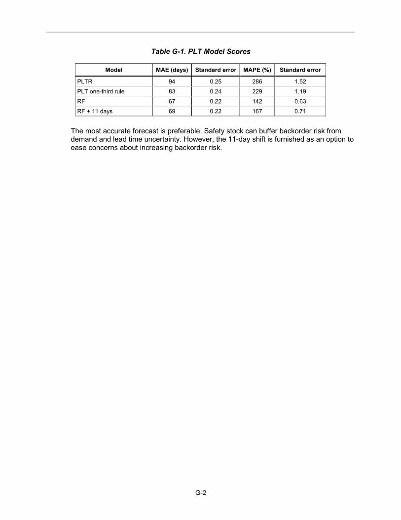
G-2

Table G-1. PLT Model Scores

Model MAE (days) Standard error MAPE (%) Standard error

PLTR 94 0.25 286 1.52 PLT one-third rule 83 0.24 229 1.19 RF 67 0.22 142 0.63 RF + 11 days 69 0.22 167 0.71

The most accurate forecast is preferable. Safety stock can buffer backorder risk from demand and lead time uncertainty. However, the 11-day shift is furnished as an option to ease concerns about increasing backorder risk.

H-1

Appendix H Magnitude and Direction of Error by Procurement Frequency

Figure H-1 shows the magnitude and direction of errors for TLTR for each of the procurement frequency bins. The baseline TLTR model tends to overpredict more than underpredict for all procurement frequencies.

Figure H-1. TLTR Magnitude and Direction of Error by Procurement Frequency

Figure H-2 shows the magnitude and direction of errors for the one-third rule for each of the procurement frequency bins. The baseline one-third rule model has the largest skew toward overprediction for infrequently procured items.

0%

10%

20%

30%

40%

50%

60%

70%

80%

90%

100%

One-timebuy

Rare Every 2years

Annually Twice a year Quarterly Monthly

Tota

l rec

ords

Model

> 6 months over

> 1 month over

> 7 days over

± 7 days

> 7 days under

> 1 month under

> 6 months under

H-2

Figure H-2. ALT One-Third Rule + PLT One-Third Rule Magnitude and Direction of Error by Procurement Frequency

Figure H-3 shows the magnitude and direction of errors for the composite RF model for each of the procurement frequency bins. The composite RF model tends to underestimate more than overestimate for all procurement frequency bins.

Figure H-3. ALT RF + PLT RF Magnitude and Direction of Error by Procurement Frequency

0%

10%

20%

30%

40%

50%

60%

70%

80%

90%

100%

One-timebuy

Rare Every 2years


Tota

l rec

ords

Model

> 6 months over

> 1 month over

> 7 days over

± 7 days

> 7 days under

> 1 month under

> 6 months under

0%

10%

20%

30%

40%

50%

60%

70%

80%

90%

100%

One-timebuy

Rare Every 2years


Tota

l rec

ords

Model

> 6 months over

> 1 month over

> 7 days over

± 7 days

> 7 days under

> 1 month under

> 6 months under

I-1

Appendix I Abbreviations

AAC acquisition advice code ADQ annual demand quantity AI artificial intelligence ALRE aircraft launch and recovery equipment ALT administrative lead time ALTR administrative lead time of record AMC acquisition method code AMSC acquisition method suffix code CAGE Commercial and Government Entity DLA Defense Logistics Agency DODAAC Department of Defense activity address code DORRA DLA Operations Research and Resource Analysis DT decision tree DVD direct vendor delivery EDW Enterprise Data Warehouse FAT first article test FINISIM™ Financial and Inventory Simulation Model™ FSC federal supply code FSG federal supply group INC item name category LASSO least absolute shrinkage and selection operator LR linear regression LTC long-term contract MAE mean absolute error MAPE mean absolute percentage error ML machine learning MSE mean squared error NAIC North American Industrial Classification NIIN National Item Identification Number

I-2

NN neural network PIIN Procurement Instrument Identification Number PLT production lead time PLTR production lead time of record PNG™ Peak Policy and Next Generation™ PO purchase order PPA power purchase agreement PPI producer price index PR purchase request R&D research and development RF random forest SPIIN supplementary procurement instrument identification number SS safety stock TLT total lead time TLTR total lead time of record UMMIPS Uniform Materiel Movement and Issue Priority System

CONTACT William G. Dinnison Director, Defense Agencies +1.571.633.7853 office [email protected] LMI | 7940 Jones Branch Drive, Tysons, VA 22102

About Us LMI is a consultancy dedicated to improving the business of government, drawing from deep expertise in advanced analytics, digital services, logistics, and management advisory services. Established as a private, not-for-profit organization in 1961, LMI is a trusted third party to federal civilian and defense agencies, free of commercial and political bias.

Learn more at lmi.org


© 2020 LMI. All rights reserved. 11509.000.00L1

June 2020

ee

Lead Time Estimation Using Artificial Intelligence

Documents

Transcript of Lead Time Estimation Using Artificial Intelligence