LAX PAIR EQUATIONS AND CONNES-KREIMER RENORMALIZATION 1. Introduction In the

LAX PAIR EQUATIONS AND CONNES-KREIMER

RENORMALIZATION

GABRIEL BADITOIU AND STEVEN ROSENBERG

Abstract. We find a Lax pair equation corresponding to the Connes-Kreimer Birkhoff

factorization of the character group of a Hopf algebra. This flow preserves the locality of

counterterms. In particular, we obtain a flow for the character given by Feynman rules,

and relate this flow to the Renormalization Group Flow.

1. Introduction

In the theory of integrable systems, many classical mechanical systems are described by

a Lax pair equation associated to a coadjoint orbit of a semisimple Lie group, for example

via the Adler-Kostant-Symes theorem [1]. Solutions are given by a Birkhoff factorization

on the group, and in some cases this technique extends to loop group formulations of

physically interesting systems such as the Toda lattice [9, 13]. By the work of Connes-

Kreimer [2], there is a Birkhoff factorization of characters on general Hopf algebras, in

particular on the Kreimer Hopf algebra of 1PI Feynman diagrams. In this paper, we

reverse the usual procedure in integrable systems: we construct a Lax pair equationdLdt

= [L,M ] on the Lie algebra of infinitesimal characters of the Hopf algebra whose

solution is given precisely by the Connes-Kreimer Birkhoff factorization (Theorem 5.9).

The Lax pair equation is nontrivial in the sense that it is not an infinitesimal inner

automorphism. The main technical issue, that the Lie algebra of infinitesimal characters

is not semisimple, is overcome by passing to the double Lie algebra with the simplest

possible Lie algebra structure. In particular, the Lax pair equation induces a flow for the

character given by Feynman rules in dimensional regularization. This flow has the physical

significance that it preserves locality, the independence of the character’s counterterm

from the mass parameter. The flow also induces Lax pair flows for the β-functions of

characters.

In §§1-4, we introduce a method to produce a Lax pair on any Lie algebra from equations

of motion on the double Lie algebra. In §5, we apply this method to the particular case

of the Lie algebra of infinitesimal characters of a Hopf algebra, and prove Theorem 5.9.

Although we focus on the minimal subtraction scheme for simplicity, the main results

hold in any renormalization scheme.

In §§6-8, we discuss physical implications of the Lax pair flow. These implications are

of two types: results in §7 which say that local characters remain local under the flow,

Date: March 2010. AMS classification: 81T15,17B80. Keywords: Renormalization, Lax pair equa-

tions, Hopf algebras. Published in Communications in Mathematical Physics 296(2010), no. 3, 655-680,

DOI: 10.1007/s00220-010-1034-7. This version is different from the published version.1

http://dx.doi.org/10.1007/s00220-010-1034-7

2 GABRIEL BADITOIU AND STEVEN ROSENBERG

and results in §8 which compare the Lax pair flow to the Renormalization Group Flow

(RGF) usually considered in quantum field theory.

As discussed in the beginning of §6, the RGF is a flow on the group GC of scalar valued

(i.e renormalized) characters on the Hopf algebra of Feynman diagrams, while the Lax

pair flow is on the Lie algebra gA of infinitesimal characters with values in Laurent series.

There are several ways to compare the RGF to the Lax pair flow, all of which involve

some identifications of the different spaces for the flows.

Working at the group level, we can consider an unrenormalized character ϕ (e.g. before

dimensional regularization and minimal subtraction) as an element of the corresponding

group GA. Manchon’s bijection [12] R : GA → gA transfers ϕ to an infinitesimal character

R(ϕ); this bijection has better behavior than the logarithm map. This infinitesimal

character has a Lax pair flow, which we can then transfer back to GA to obtain a flow ϕt.

Finally, we can compare the flow of the renormalized scalar valued characters (ϕt)+(0) in

Connes-Kreimer notation to the RGF of ϕ+(0). However, even in simple examples these

two flows are not the same.

Working at the infinitesimal level, we consider the β-function of a renormalized char-

acter, since the β-function is essentially the infinitesimal generator of the RGF. The

β-function of a character is an element of the Lie algebra gC of scalar valued characters,

so in §6 we extend the β-function to a β-character in gA. (This extension has previously

appeared in the literature in a different context.) This material is used in the main results

in §7-8.

In preparation for the study of the RGF, in §7 we discuss “how physical” the Lax pair

flow is. We first show that the Lax pair flow is trivial on primitives in the Hopf algebra. We

then prove the main result (Theorem 7.3) that local characters for the minimal subtraction

scheme remain local under the Lax pair flow, so the flow stays inside the set of physically

plausible characters. We also discuss the dependence of this result on the renormalization

scheme, and identify characters for which the Lax pair flow is trivial.

From the results in §7, it seems unlikely that one can directly identify the RGF with

a Lax pair flow, so in §8 we track how the RGF changes under the Lax pair flow. For

example, even if the Lax pair flow is nontrivial for a given initial physically plausible

character, one might hope that the RGF is unchanged. In §8, we give a criterion (Corollary

8.4) for when the RGF is fixed under the Lax pair flow. We show that the β-character and

the β-function satisfy Lax pair equations, and briefly discuss the complete integrability

of Lax pair flows of characters and β-functions.

We would like to thank Dirk Kreimer for suggesting we investigate the connection

between the Connes-Kreimer factorization and integrable systems, Dominique Manchon

for helpful conversations, and the referee for valuable suggestions.

2. The double Lie algebra and its associated Lie Group

There is a well known method to associate a Lax pair equation to a Casimir element

on the dual g∗ of a semisimple Lie algebra g [13]. The semisimplicity is used to produce

an Ad-invariant, symmetric, non-degenerate bilinear form on g, allowing an identification

LAX PAIR EQUATIONS AND CONNES-KREIMER RENORMALIZATION 3

of g with g∗. For a general Lie algebra g, there may be no such bilinear form. To produce

a Lax pair, we need to extend g to a larger Lie algebra with the desired bilinear form.

We do this by constructing a Lie bialgebra structure on g, whose definition we now recall

(see e.g. [10]).

Definition 2.1. A Lie bialgebra is a Lie algebra (g, [·, ·]) with a linear map γ : g → g⊗ g

such that

a) tγ : g∗ ⊗ g∗ → g∗ defines a Lie bracket on g∗,

b) γ is a 1-cocycle of g, i.e.

ad(2)x (γ(y))− ad(2)

y (γ(x))− γ([x, y]) = 0,

where ad(2)x : g ⊗ g → g⊗ g is given by ad(2)

x (y ⊗ z) = adx(y)⊗ z + y ⊗ adx(z) =

[x, y]⊗ z + y ⊗ [x, z].

A Lie bialgebra (g, [·, ·], γ) induces an Lie algebra structure on the double Lie algebra

g⊕ g∗ by

[X, Y ]g⊕g∗ = [X, Y ],

[X∗, Y ∗]g⊕g∗ = tγ(X ⊗ Y ),

[X, Y ∗] = ad∗X(Y

∗),

for X , Y ∈ g and X∗, Y ∗ ∈ g∗, where ad∗ is the coadjoint representation given by

ad∗X(Y

∗)(Z) = −Y ∗(adX(Z)) for Z ∈ g.

Since it is difficult to construct explicitly the Lie group associated to the Lie algebra

g⊕ g∗, we will choose the trivial Lie bialgebra given by the cocycle γ = 0 and denote by

δ = g ⊕ g∗ the associated Lie algebra. Let Yi, i = 1, . . . , l be a basis of g, with dual

basis Y ∗i . The Lie bracket [·, ·]δ on δ is given by

[Yi, Yj]δ = [Yi, Yj], [Y∗i , Y

∗j ]δ = 0, [Yi, Y

∗j ]δ = −

∑

k

cjikY∗k ,

where the cjik are the structure constants: [Yi, Yj] =∑

k ckijYk. The Lie group naturally

associated to δ is given by the following proposition.

Proposition 2.2. Let G be the simply connected Lie group with Lie algebra g and let

θ : G × g∗ → g∗ be the coadjoint representation θ(g,X) = Ad∗G(g)(X). Then the Lie

algebra of the semi-direct product G = G⋉θ g∗ is the double Lie algebra δ.

Proof. The Lie group law on the semi-direct product G is given by

(g,X) · (g′, X ′) = (gg′, X + θ(g,X ′)).

Let g be the Lie algebra of G. Then the bracket on g is given by

[X, Y ∗]g = dθ(X, Y ∗), [X, Y ]g = [X, Y ], [X∗, Y ∗]g = 0,

for left-invariant vector fields X , Y of G and X∗, Y ∗ ∈ g∗. We have dθ(X, Y ∗) =

dAd∗G(X)(Y ∗) = [X, Y ∗]δ since dAdG = adg.

The main point of this construction is existence of a good bilinear form on the double.


Lemma 2.3. The natural pairing 〈·, ·〉 : δ ⊗ δ → C given by

〈(a, b∗), (c, d∗)〉 = d∗(a) + b∗(c), a, c ∈ g, b∗, d∗ ∈ g∗,

is an Ad-invariant symmetric non-degenerate bilinear form on the Lie algebra δ.

Proof. By [10], this bilinear form is ad-invariant. Since G is simply connected, the Ad-

invariance follows. As an explicit example, we have

AdG((g, 0))(Yi, 0) = (AdG(g)(Yi), 0), and AdG((g, 0))(0, Y∗j ) = (0,Ad∗

G(g)(Y∗j )),

from which the invariance under AdG(g, 0) follows.

3. The loop algebra of a Lie algebra

Following [1], we consider the loop algebra

Lδ = L(λ) =

N∑

j=M

λjLj | M,N ∈ Z, Lj ∈ δ.

The natural Lie bracket on Lδ is given by[

∑

λiLi,∑

λjL′j

]

=∑

k

λk∑

i+j=k

[Li, L′j].

Set

Lδ+ = L(λ) =N∑

j=0

λjLj | N ∈ Z+ ∪ 0, Lj ∈ δ

Lδ− = L(λ) =−1∑

j=−M

λjLj | M ∈ Z+, Lj ∈ δ.

Let P+ : Lδ → Lδ+ and P− : Lδ → Lδ− be the natural projections and set R = P+ − P−.

The natural pairing 〈·, ·〉 on δ yields an Ad-invariant, symmetric, non-degenerate pairing

on Lδ by setting⟨

N∑

i=M

λiLi,

N ′

∑

j=M ′

λjL′j

⟩

=∑

i+j=−1

〈Li, L′j〉.

For our choice of basis Yi of g, we get an isomorphism

(3.1) I : L(δ∗) → Lδ

with

I(

∑

LjiYjλ

i)

=∑

LjiY

∗j λ

−1−i.

We will need the following lemmas.

Lemma 3.1. [1] We have the following natural identifications:

Lδ+ = L(δ∗)− and Lδ− = L(δ∗)+.


Lemma 3.2. [13, Lem. 4.1] Let ϕ be an Ad-invariant polynomial on δ. Then

ϕm,n[L(λ)] = Resλ=0(λ−nϕ(λmL(λ)))

is an Ad-invariant polynomial on Lδ for m,n ∈ Z.

As a double Lie algebra, δ has an Ad-invariant polynomial, the quadratic polynomial

ψ(Y ) = 〈Y, Y 〉

associated to the natural pairing. Let Yl+i = Y ∗i for i ∈ 1, . . . , l = dim(g), so elements

of Lδ can be written L(λ) =2l∑

j=1

N∑

i=−M

LjiYjλ

i. Then the Ad-invariant polynomials

(3.2) ψm,n(L(λ)) = Resλ=0(λ−nψ(λmL(λ))),

defined as in Lemma 3.2 are given by

(3.3) ψm,n(L(λ)) = 2

l∑

j=1

∑

i+k−n+2m=−1

LjiL

j+lk .

Note that powers of ψ are also Ad-invariant polynomials on δ, so

(3.4) ψkm,n(L(λ)) = Resλ=0(λ

−nψk(λmL(λ)))

are Ad-invariant polynomials on Lδ. It would be interesting to classify all Ad-invariant

polynomials on Lδ in general.

4. The Lax pair equation

Let P+, P− be endomorphisms of a Lie algebra h and set R = P+ − P−. Assume that

[X, Y ]R = [P+X,P+Y ]− [P−X,P−Y ]

is a Lie bracket on h. From [13, Theorem 2.1], the equations of motion induced by a

Casimir (i.e. Ad-invariant) function ϕ on h∗ are given by

(4.1)dL

dt= −ad∗

hM · L,

for L ∈ h∗, where M = 12R(dϕ(L)) ∈ h.

Now we take h = (Lδ)∗ = L(δ∗), with δ a finite dimensional Lie algebra and with the

understanding that (Lδ)∗ is the graded dual with respect to the standard Z-grading on

Lδ. Let P± be the projections of Lδ∗ onto Lδ∗±. After identifying Lδ∗ = Lδ and ad∗ = −ad

via the map I in (3.1), the equations of motion (4.1) can be written in Lax pair form

(4.2)dL

dt= [M,L],

where M = 12R(I(dϕ(L(λ)))) ∈ Lδ, and ϕ is a Casimir function on Lδ∗ = Lδ [13,

Theorem 2.1]. Finding a solution for (4.2) reduces to the Riemann-Hilbert (or Birkhoff)

factorization problem. The following theorem is a corollary of [1, Theorem 4.37] [13,

Theorem 2.2].


Theorem 4.1. Let ϕ be a Casimir function on Lδ and set X = I(dϕ(L(λ))) ∈ Lδ, for

L(λ) = L(0)(λ) ∈ Lδ. Let g±(t) be the smooth curves in LG which solve the factorization

problem

exp(−tX) = g−(t)−1g+(t),

with g±(0) = e, and with g+(t) = g+(t)(λ) holomorphic in λ ∈ C and g−(t) a polynomial

in 1/λ with no constant term. Let M = 12R(I(dϕ(L(λ)))) ∈ Lδ. Then the integral curve

L(t) of the Lax pair equation

dL

dt= [L,M ]

is given by

(4.3) L(t) = AdLGg±(t) · L(0).

This Lax pair equation projects to a Lax pair equation on the loop algebra of the

original Lie algebra g. Let π1 be either the projection of G onto G or its differential from

δ onto g. This extends to a projection of Lδ onto Lg. The projection of (4.2) onto Lg is

(4.4)d(π1(L(t)))

dt= [π1(L), π1(M)],

since π1 = dπ1 commutes with the bracket. Thus the equations of motion (4.2) induce a

Lax pair equation on Lg, although this is not the equations of motion for a Casimir on

Lg.

Theorem 4.2. The Lax pair equation of Theorem 4.1 projects to a Lax pair equation on

Lg.

Remark 4.3. The content of this theorem is that a Lax pair equation on the Lie algebra

of a semi-direct product G ⋉ G′ evolves on an adjoint orbit, and the projection onto

g evolves on an adjoint orbit and is still in Lax pair form. Lax pair equations often

appear as equations of motion for some Hamiltonian, but the projection may not be the

equations of motion for any function on the smaller Lie algebra. We thank B. Khesin for

this observation.

When ψm,n is the Casimir function on Lδ given by (3.2), X can be written nicely in

terms of L(λ).

Proposition 4.4. Let X = I(dψm,n(L(λ))). Then

(4.5) X = 2λ−n+2mL(λ).

Proof. Write L(λ) =∑

i,j

Ljiλ

iYj. By formula (3.3), we have

(4.6)∂ψm,n

∂Ltp

=

2Lt+ln−1−2m−p, if t ≤ l

2Lt−ln−1−2m−p, if t > l.


Therefore

X = I(dψm,n(L(λ))) =∑

p,t

∂ψm,n

∂Ltp

λ−1−pY ∗t

= 2λ−n+2m∑

p

(

l∑

t=1

Lt+ln−1−2m−pYt+lλ

n−1−2m−p +2l∑

t=l+1

Lt−ln−1−2m−pYt−lλ

n−1−2m−p

)

= 2λ−n+2mL(λ).

5. The main theorem for Hopf algebras

In this section we give formulas for the Birkhoff decomposition of a loop in the Lie

group of characters of a Hopf algebra and produce the Lax pair equations associated to

the Birkhoff decomposition. We present two approaches, both motivated by the Connes-

Kreimer Hopf algebra of 1PI Feynman graphs. First, in analogy to truncating Feynman

integral calculations at a certain loop level, we truncate a (possibly infinitely generated)

Hopf algebra to a finitely generated Hopf algebra, and solve Lax pair equations on the

finite dimensional piece (Theorem 5.4). We also discuss the compatibility of solutions

related to different truncations. Second, we solve a Lax pair equation associated to Ad-

covariant maps on the full Hopf algebra (Theorem 5.9). These results are proven for the

minimal subtraction scheme, but apply to other renormalization schemes.

In Section 5.1, we introduce notation and prove a Birkhoff decomposition for the loop

group associated to a doubled Lie algebra. In Section 5.2, we introduce the truncation

process and prove Theorem 5.4. In Section 5.3, we treat the Feynman rules character and

prove Theorem 5.9. In Section 5.4, we note that the methods of this section apply to any

renormalization scheme given by a linear projection satisfying the Rota-Baxter equation.

5.1. Birkhoff decompositions for doubled Lie algebras. Let H = (H, 1, µ,∆, ε, S)

be a graded connected Hopf algebra over C. Let A be a unital commutative algebra with

unit 1A. Unless stated otherwise, A will be the algebra of Laurent series; the only other

occurrence in this paper is A = C.

Definition 5.1. The character group GA of the Hopf algebra H is the set of algebra

morphisms φ : H → A with φ(1) = 1A. The group law is given by the convolution product

(ψ1 ⋆ ψ2)(h) = 〈ψ1 ⊗ ψ2,∆h〉;

the unit element is ε.

Definition 5.2. An A-valued infinitesimal character of a Hopf algebra H is a C-linear

map Z : H → A satisfying

〈Z, hk〉 = 〈Z, h〉ε(k) + ε(h)〈Z, k〉.

The set of infinitesimal characters is denoted by gA and is endowed with a Lie algebra

bracket:

[Z,Z ′] = Z ⋆ Z ′ − Z ′ ⋆ Z, for Z, Z ′ ∈ gA,


where 〈Z ⋆ Z ′, h〉 = 〈Z ⊗ Z ′,∆(h)〉. Notice that Z(1) = 0.

For a finitely generated Hopf algebra, GC is a Lie group with Lie algebra gC, and for

any Hopf algebra and any A, the same is true at least formally.

We recall that δ = gC ⊕ g∗Cis the double of gC and the g∗

Cis the graded dual of gC. We

consider the algebra Ωδ = δ ⊗A of formal Laurent series with values in δ

Ωδ = L(λ) =∞∑

j=−N

λjLj | Lj ∈ δ, N ∈ Z.

The natural Lie bracket on Ωδ is[

∑

λiLi,∑

λjL′j

]

=∑

k

λk∑

i+j=k

[Li, L′j].

Set

Ωδ+ = L(λ) =

∞∑

j=0

λjLj | Lj ∈ δ

Ωδ− = L(λ) =

−1∑

j=−N

λjLj | Lj ∈ δ, N ∈ Z+.

Recall that for any Lie group K, a loop L(λ) with values in K has a Birkhoff decom-

position if L(λ) = L(λ)−1− L(λ)+ with L(λ)−1

− holomorphic in λ−1 ∈ P1 − 0 and L(λ)+holomorphic in λ ∈ P1 − ∞. In the next lemma, G refers to G⋉θ g

∗ as in Prop. 2.2.

We prove the existence of a Birkhoff decomposition for any element (g, α) ∈ ΩG.

Theorem 5.3. Every (g, α) ∈ ΩG = GA ⋉Ad∗GA

g∗A has a Birkhoff decomposition (g, α) =

(g−, α−)−1(g+, α+) with (g+, α+) holomorphic in λ and (g−, α−) a polynomial in λ−1 with-

out constant term.

Proof. We recall that (g1, α1)(g2, α2) = (g1g2, α1 +Ad∗(g1)(α2)). Thus

(g, α) = (g−, α−)−1(g+, α+) if and only if g = g−1

− g+ and α = Ad∗(g−1− )(−α− + α+).

Let g = g−1− g+ be the Birkhoff decomposition of g in GA given in [2, 6, 12]. Set

α+ = P+(Ad∗(g−)(α)) and α− = −P−(Ad

∗(g−)(α)), where P+ and P− are the holo-

morphic and pole part, respectively. Then for this choice of α+ and α−, we have (g, α) =

(g−, α−)−1(g+, α+). Note that the Birkhoff decomposition is unique.

5.2. Lax pair equations for the truncated Lie algebra of infinitesimal characters.

For a finitely generated Hopf algebra, we can apply Theorems 4.1, 4.2 to produce a Lax

pair equation on Lδ and on the loop space of infinitesimal characters Lg. However,

the common Hopf algebras of 1PI Feynman diagrams and rooted trees are not finitely

generated.

As we now explain, we can truncate the Hopf algebra to a finitely generated Hopf alge-

bra, and use the Birkhoff decomposition to solve a Lax pair equation on the infinitesimal

character group of the truncation. A graded Hopf algebra H = ⊕n∈NHn is said to be

of finite type if each homogeneous component Hn is a finite dimensional vector space.


Let B = Tii∈N be a minimal set of homogeneous generators of the Hopf algebra H such

that deg(Ti) ≤ deg(Tj) if i < j and such that T0 = 1. For i > 0, we define the C-valued

infinitesimal character Zi on generators by Zi(Tj) = δij . The Lie algebra of infinitesimal

characters g is a graded Lie algebra generated by Zii>0. Let g(k) be the vector space

generated by Zi | deg(Ti) ≤ k. We define deg(Zi) = deg(Ti) and set

[Zi, Zj]g(k) =

[Zi, Zj] if deg(Zi) + deg(Zj) ≤ k

0 if deg(Zi) + deg(Zj) > k

We identify ϕ ∈ GC with ϕ(Ti) ∈ CN and on CN we set a group law given by ϕ1(Ti)⊕

ϕ2(Ti) = (ϕ1 ⋆ ϕ2)(Ti). G(k) = ϕ(Ti)i | deg(Ti)≤k | ϕ ∈ GC is a finite dimensional

Lie subgroup of GC = (CN,⊕) and the Lie algebra of G(k) is g(k). There is no loss of

information under this identification, as ϕ(TiTj) = ϕ(Ti)ϕ(Tj).

Let δ(k) be the double Lie algebra of g(k) and let G(k) be the simply connected Lie group

with Lie(G(k)) = δ(k) as in Proposition 2.2. The following theorem is a restatement of

Theorem 4.1 in our new setup.

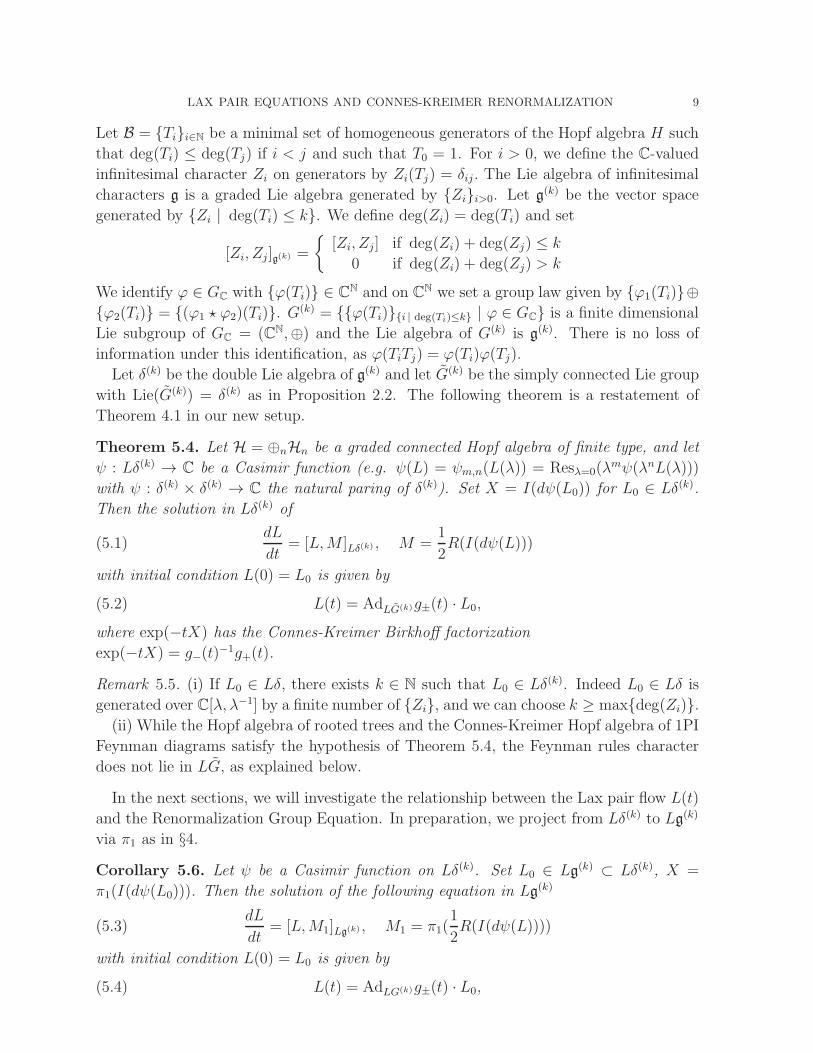
Theorem 5.4. Let H = ⊕nHn be a graded connected Hopf algebra of finite type, and let

ψ : Lδ(k) → C be a Casimir function (e.g. ψ(L) = ψm,n(L(λ)) = Resλ=0(λmψ(λnL(λ)))

with ψ : δ(k) × δ(k) → C the natural paring of δ(k)). Set X = I(dψ(L0)) for L0 ∈ Lδ(k).

Then the solution in Lδ(k) of

(5.1)dL

dt= [L,M ]Lδ(k) , M =

1

2R(I(dψ(L)))

with initial condition L(0) = L0 is given by

(5.2) L(t) = AdLG(k)g±(t) · L0,

where exp(−tX) has the Connes-Kreimer Birkhoff factorization

exp(−tX) = g−(t)−1g+(t).

Remark 5.5. (i) If L0 ∈ Lδ, there exists k ∈ N such that L0 ∈ Lδ(k). Indeed L0 ∈ Lδ is

generated over C[λ, λ−1] by a finite number of Zi, and we can choose k ≥ maxdeg(Zi).

(ii) While the Hopf algebra of rooted trees and the Connes-Kreimer Hopf algebra of 1PI

Feynman diagrams satisfy the hypothesis of Theorem 5.4, the Feynman rules character

does not lie in LG, as explained below.

In the next sections, we will investigate the relationship between the Lax pair flow L(t)

and the Renormalization Group Equation. In preparation, we project from Lδ(k) to Lg(k)

via π1 as in §4.

Corollary 5.6. Let ψ be a Casimir function on Lδ(k). Set L0 ∈ Lg(k) ⊂ Lδ(k), X =

π1(I(dψ(L0))). Then the solution of the following equation in Lg(k)

(5.3)dL

dt= [L,M1]Lg(k) , M1 = π1(

1

2R(I(dψ(L))))


(5.4) L(t) = AdLG(k)g±(t) · L0,


where exp(−tX) has the Connes-Kreimer Birkhoff factorization in Lg(k)

exp(−tX) = g−(t)−1g+(t).

Remark 5.7. (i) For Feynman graphs, this truncation corresponds to halting calculations

after a certain loop level. From our point of view, this truncation is somewhat crude.

g(k) is not a subalgebra of g, and if k < ℓ, g(k) is not a subalgebra of g(ℓ). Although

the Casimirs ψm,n and the exponential map restrict well from g to g(k), the Birkhoff

decomposition exp(−tX) of X ∈ Lg(k) is very different from the Birkhoff decompositions

in Lg, Lg(ℓ). In fact, if g ∈ G(k) has Birkhoff decomposition g = g−1− g+ in G, there does

not seem to be f(k) ∈ N such that g± ∈ G(f(k)).

(ii) It would interesting to know, especially for the Hopf algebras of Feynman graphs or

rooted trees, whether there exists a larger connected graded Hopf algebra H′ containing

H such that the associated infinitesimal Lie algebra Lie(G′C) is the double δ. This would

provide a Lax pair equation associated to an equation of motion on the infinitesimal Lie

algebra of H′. The most natural candidate, the Drinfeld double D(H) of H, does not work

since the dimension of the Lie algebra associated to D(H) is larger than the dimension of

δ.

5.3. Lax pair equations in the general case. In [2], Connes and Kreimer give a

Birkhoff decomposition for the character group of the Hopf algebra of 1PI graphs, and

in particular for the Feynman rules character ϕ(λ) given by minimal subtraction and

dimensional regularization. The truncation process treated above does not handle the

Feynman rules character, as the regularized toy model character defined in [5, 7, 11] of

the Hopf algebra of integer decorated rooted trees and the Feynman rules character are

not polynomials in λ, λ−1, but Laurent series in λ. Thus Corollary 5.6 does not apply,

as in our notation log(ϕ(λ)) ∈ Ωg \ Lg. This and Remark 5.7(i) force us to consider a

direct approach in Ωg as in the next theorem. However, we cannot expect that the Lax

pair equation is associated to any Hamiltonian equation, and we replace Casimirs with

Ad-covariant functions.

Definition 5.8. [14] Let G be a Lie group with Lie algebra g. A map f : g → g is

Ad-covariant if Ad(g)(f(L)) = f(Ad(g)(L)) for all g ∈ G, L ∈ g.

Theorem 5.9. Let H be a connected graded commutative Hopf algebra with gA the associ-

ated Lie algebra of infinitesimal characters with values in Laurent series. Let f : gA → gA

be an Ad-covariant map. Let L0 ∈ gA satisfy [f(L0), L0] = 0. Set X = f(L0). Then the

solution of

(5.5)dL

dt= [L,M ], M =

1

2R(f(L))


(5.6) L(t) = AdGg±(t) · L0,


exp(−tX) = g−(t)−1g+(t).


Proof. The proof is similar to [13, Theorem 2.2]. First notice that

d

dt

(

Ad(g−(t)−1g+(t)) · L0

)

=d

dt(exp(−tX)L0 exp(tX))

= − exp(−tX)XL0 exp(tX) + exp(−tX)L0X exp(tX)

= − exp(−tX)[X,L0] exp(tX) = 0,

which implies Ad(g−(t)−1g+(t)) · L0 = L0 and Ad(g−(t)) · L0 = Ad(g+(t)) · L0. Set

L(t) = Ad(g±(t)) · L0 = g±(t)L0g±(t)−1. As usual,

dL

dt=

[

dg±(t)

dtg±(t)

−1, L(t)

]

,

sodL

dt=

1

2

[

dg+(t)

dtg+(t)

−1 +dg−(t)

dtg−(t)

−1, L(t)

]

.

The Birkhoff factorization g+(t) = g−(t) exp(−tX) gives

dg+(t)

dt=dg−(t)

dtexp(−tX) + g−(t)(−X) exp(−tX),

and sodg+(t)

dtg+(t)

−1 =dg−(t)

dtg−(t)

−1 + g−(t)(−X)g−(t)−1.

Thus

2M = R(f(L(t))) = R(f(Ad(g−(t)) · L0)) = R(Ad(g−(t)) · f(L0))

= R(Ad(g−(t)) ·X)) = −R(dg+(t)

dtg+(t)

−1) +R(dg−(t)

dtg−(t)

−1)

= −dg+(t)

dtg+(t)

−1 −dg−(t)

dtg−(t)

−1.

Here we use (dg±(t)dt

g±(t)−1)(x) ∈ A± for x ∈ H. Thus dL

dt= [L,M ].

Remark 5.10. In a particular case of Theorem 5.9, we get a Hamiltonian system. First,

since the proof of Theorem 5.9 depends on the splitting gA = gA−⊕ gA+ of the Lie

algebra and the Birkhoff decomposition of the Lie group, and since this splitting and

Birkhoff decomposition exist (see Theorem 5.3) on Lδk, Theorem 5.9 extends to Lδk. Let

ψ : Lδk → C be a Casimir function on Lδk. For f(L) = (∇ψ)(L) the gradient of ψ, f is

an Ad-invariant function on Lδk. Since ψ is a Casimir function, [L, (∇ψ)(L)] = 0 for all L

(see [1, 14]), so in particular [f(L0), L0] = 0. Thus, the Hamiltonian system (5.5) satisfies

(5.6). Since I(dψ) = ∇ψ, Theorem 5.4 is a particular case of the Lδk version of Theorem

5.9. It is natural to ask if the Hamiltonian system (5.1) is completely integrable; this is

discussed briefly in §8.

If f : gA → gA is given by f(L) = 2λ−n+2mL, then f is Ad-covariant and [f(L0), L0] =

[2λ−n+2mL0, L0] = 0.


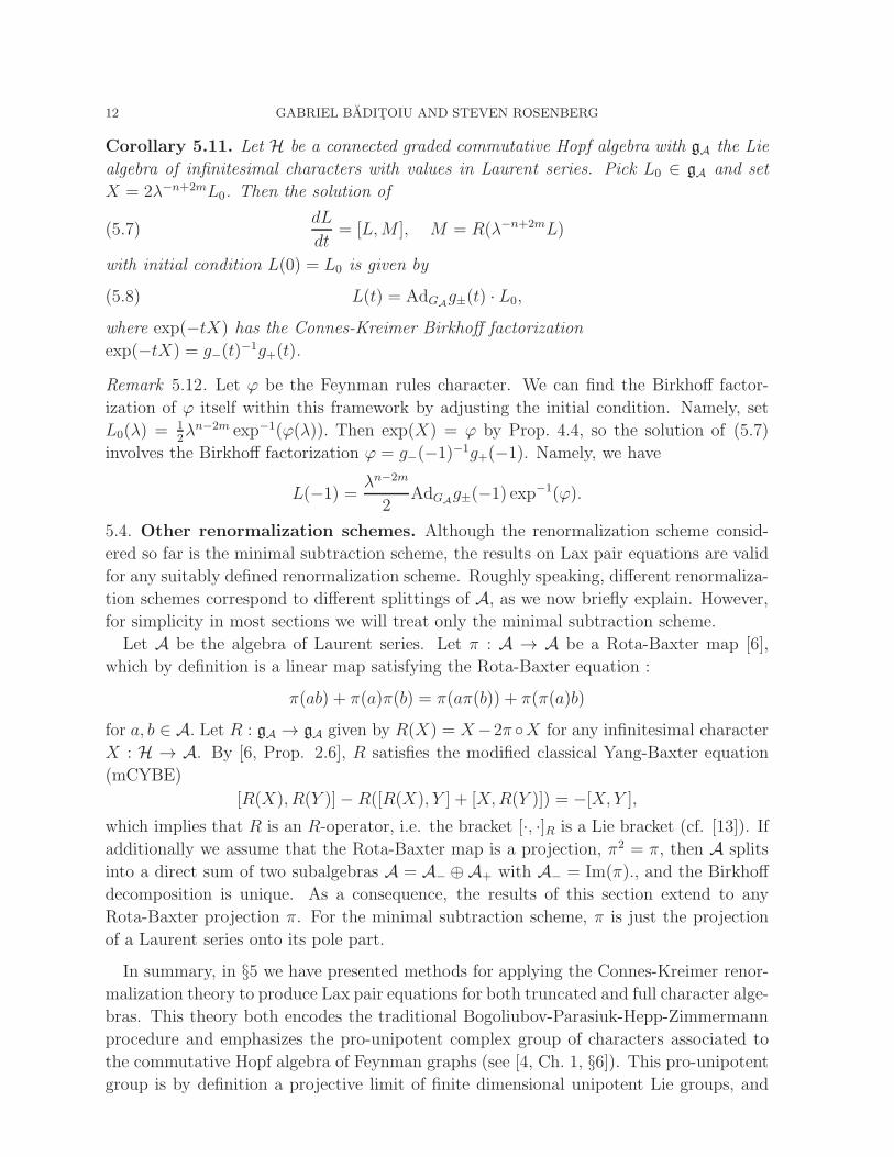
Corollary 5.11. Let H be a connected graded commutative Hopf algebra with gA the Lie

algebra of infinitesimal characters with values in Laurent series. Pick L0 ∈ gA and set

X = 2λ−n+2mL0. Then the solution of

(5.7)dL

dt= [L,M ], M = R(λ−n+2mL)


(5.8) L(t) = AdGAg±(t) · L0,


exp(−tX) = g−(t)−1g+(t).

Remark 5.12. Let ϕ be the Feynman rules character. We can find the Birkhoff factor-

ization of ϕ itself within this framework by adjusting the initial condition. Namely, set

L0(λ) = 12λn−2m exp−1(ϕ(λ)). Then exp(X) = ϕ by Prop. 4.4, so the solution of (5.7)

involves the Birkhoff factorization ϕ = g−(−1)−1g+(−1). Namely, we have

L(−1) =λn−2m

2AdGA

g±(−1) exp−1(ϕ).

5.4. Other renormalization schemes. Although the renormalization scheme consid-

ered so far is the minimal subtraction scheme, the results on Lax pair equations are valid

for any suitably defined renormalization scheme. Roughly speaking, different renormaliza-

tion schemes correspond to different splittings of A, as we now briefly explain. However,

for simplicity in most sections we will treat only the minimal subtraction scheme.

Let A be the algebra of Laurent series. Let π : A → A be a Rota-Baxter map [6],

which by definition is a linear map satisfying the Rota-Baxter equation :

π(ab) + π(a)π(b) = π(aπ(b)) + π(π(a)b)

for a, b ∈ A. Let R : gA → gA given by R(X) = X−2π X for any infinitesimal character

X : H → A. By [6, Prop. 2.6], R satisfies the modified classical Yang-Baxter equation

(mCYBE)

[R(X), R(Y )]− R([R(X), Y ] + [X,R(Y )]) = −[X, Y ],

which implies that R is an R-operator, i.e. the bracket [·, ·]R is a Lie bracket (cf. [13]). If

additionally we assume that the Rota-Baxter map is a projection, π2 = π, then A splits

into a direct sum of two subalgebras A = A− ⊕ A+ with A− = Im(π)., and the Birkhoff

decomposition is unique. As a consequence, the results of this section extend to any

Rota-Baxter projection π. For the minimal subtraction scheme, π is just the projection

of a Laurent series onto its pole part.

In summary, in §5 we have presented methods for applying the Connes-Kreimer renor-

malization theory to produce Lax pair equations for both truncated and full character alge-

bras. This theory both encodes the traditional Bogoliubov-Parasiuk-Hepp-Zimmermann

procedure and emphasizes the pro-unipotent complex group of characters associated to

the commutative Hopf algebra of Feynman graphs (see [4, Ch. 1, §6]). This pro-unipotent

group is by definition a projective limit of finite dimensional unipotent Lie groups, and


has an associated pro-nilpotent Lie algebra, a projective limit of nilpotent Lie algebras. In

our case, the finite dimensional nilpotent Lie algebras are the double of the infinitesimal

characters of the truncated Hopf algebras, and the corresponding unipotent groups are

the exponentials of the nilpotent algebras.

6. The Connes-Kreimer β-function and the β-character

6.1. Overview of §§6-8. The next three sections are devoted to studying ”how physical”

the Lax pair flow is. This vague question can be approached in at least two ways: (i)

given a property of a physically plausible character, we ask if this property is preserved

under the Lax pair flow (see §7); (ii) we compare the Lax pair flow to the renormalization

group flow (RGF) which is fundamental in quantum field theory (see §8).

Before addressing either topic, we have to recall where various flows live. A character for

us is an element of GA, the homomorphisms from the Hopf algebra of Feynman diagrams

to the algebra A of Laurent series (although many of our results hold in more generality).

A renormalized character, such as Feynman rules given by dimensional regularization and

minimal subtraction, is an element of GC, the homomorphisms from the Hopf algebra to

C. The RGF is a flow on GC. In contrast, the Lax pair flow is on the Lie algebra gA of

infinitesimal characters, which is formally the Lie algebra of GA.

As an example of topic (i), in §7 we ask if the physically necessary property of locality

(see Def. 6.2) of an unrenormalized character ϕ ∈ GA is preserved under the Lax pair

flow. To make sense of this question, we must choose a bijection α : GA → gA, take

α(ϕ) ∈ gA, let α(ϕ) flow to L(t) under the Lax pair flow, and set ϕt = α−1(L(t)). The

question, ”If ϕ is local, is ϕt local,” is now well defined but depends on the choice of

α and a choice of Casimir function for the Lax pair flow. A natural choice of α is the

logarithm, the inverse of the exponential map, but it turns out that another bijection due

to Manchon has much better behavior.

As an example of (ii), we can ask to what extent the RGF is related to the Lax pair flow.

Since these flows live on different spaces, there are several ways to interpret this question,

and each interpretation involves a choice of identification. For example, we can ask if

the family of renormalized scalar characters [α−1(L(t))]+(λ = 0) ∈ GC ever coincides the

RGF of a character ϕ ∈ GA. The answer to this is negative for the bijections mentioned

above.

Since the RGF does not equal the Lax pair flow under these identifications, it is better

to ask how the RGF is affected by the Lax pair flow. In particular, we consider the

β-function β = βϕ ∈ gC, the infinitesimal generator of the RGF. We can extend β to an

element β ∈ gA, and ask for the behavior of β under the Lax pair flow. We show in §8

that β and hence β satisfy a Lax pair flow. This allows us to give a fixed point equation

(Corollary 8.4) which has a solution iff the RGF of (suitably identified) ϕt coincide.

In summary, we will see in §7 that the physically important property of locality is

preserved under the Lax pair flow. After preliminary work in §6 on the β-character, we

will see in §8 that the RGF of a family of characters ϕt given by a Lax pair flow is itself

controlled by a Lax pair flow.


6.2. The β-character. As mentioned above, we extend the (scalar) β-function βϕ ∈ gC

of a local character ϕ to an infinitesimal character βϕ ∈ gA (Lemma 6.6). This “β-

character” has already appeared in the literature: βϕ = λR(ϕ), in the language of [12]

explained below (Lemma 6.7).

To define the β-character, we recall material from [3, 7, 12]. Throughout this section,

A denotes the algebra of Laurent series.

Let H =⊕

n

Hn be a connected graded Hopf algebra. Let Y be the biderivation on H

given on homogeneous elements by

Y : Hn → Hn, Y (x) = nx for x ∈ Hn.

Definition 6.1. [12] We define the bijection R : GA → gA by

R(ϕ) = ϕ−1 ⋆ (ϕ Y ).

We now define an action of C on GA. For s ∈ C and ϕ ∈ GA we define ϕs(x) on an

homogeneous element x ∈ H by

(6.1) ϕs(x)(λ) = esλ|x|ϕ(x)(λ),

for any λ ∈ C, where |x| is the degree of x.

Definition 6.2. Let

(6.2) GΦA = ϕ ∈ GA

∣

∣

d

ds(ϕs)− = 0,

be the set of characters with the negative part of the Birkhoff decomposition independent

of s. Elements of GΦA are called local characters.

The dimensional regularized Feynman rule character ϕ is local. Referring to [3, 7], the

physical meaning of locality is that the counterterm ϕ− does not depend on the mass

parameter µ: ∂ϕ−

∂µ= 0, and this in turn reflects the locality of the Lagrangian.

Proposition 6.3 ([3, 12, 7]). Let ϕ ∈ GΦA. Then the limit

Fϕ(s) = limλ→0

ϕ−1(λ) ⋆ ϕs(λ)

exists and is a one-parameter subgroup in GA ∩GC of scalar valued characters of H.

Notice that (ϕ−1(λ) ⋆ ϕs(λ))(Γ) ∈ A+ as

ϕ−1(λ) ⋆ ϕs(λ) = ϕ−1+ ⋆ ϕ− ⋆ (ϕ

s)−1− ⋆ (ϕs)+ = ϕ−1

+ ⋆ (ϕs)+.

Definition 6.4. For ϕ ∈ GΦA, the β-function of ϕ is defined to be βϕ = −(Res(ϕ−)) Y ).

We have [3]

βϕ =d

ds

∣

∣

∣

s=0Fϕ−1

−(s),

where Fϕ−1−, the one-parameter subgroup associated to ϕ−1

− , also belongs to GΦA.

To relate the β-function βϕ ∈ gC to our Lax pair equations, which live on gA, we can

either consider gC as a subset of gA, or we can extend βϕ to an element of gA. Since gC is

not preserved under the Lax pair flow, we take the second approach.


Definition 6.5. For ϕ ∈ GΦA, x ∈ H , set

βϕ(x)(λ) =d

ds

∣

∣

∣

s=0(ϕ−1 ⋆ ϕs)(x)(λ).

The following lemma establishes that β is an infinitesimal character.

Lemma 6.6. Let ϕ ∈ GΦA.

i) βϕ is an infinitesimal character in gA.

ii) βϕ is holomorphic (i.e. βϕ(x) ∈ A+ for any x).

Proof. i) For two homogeneous elements x, y ∈ H, we have:

ϕs(xy) = es|xy|λϕ(xy) = es|x|λϕ(x)es|y|λϕ(y) = ϕs(x)ϕs(y).

Therefore ϕ−1 ⋆ ϕs ∈ GA. Since ϕ−1 ⋆ ϕ0 = e we get

d

ds

∣

∣

∣

s=0ϕ−1 ⋆ ϕs ∈ gA.

ii) Since dds(ϕs)− = 0, we get

βϕ =d

ds

∣

∣

∣

s=0

(

(ϕ+)−1 ⋆ ϕ− ⋆ ((ϕ

s)−)−1 ⋆ (ϕs)+

)

= (ϕ+)−1 ⋆

d

ds

∣

∣

∣

s=0(ϕs)+.

Then

βϕ(x) = (ϕ+)−1(x′)

d

ds

∣

∣

∣

s=0(ϕs)+(x

′′) = (ϕ+)(S(x′))

d

ds

∣

∣

∣

s=0(ϕs)+(x

′′)

Therefore βϕ(x) ∈ A+.

Lemma 6.7. If ϕ ∈ GΦA then

(i) βϕ = λR(ϕ),

(ii) βϕ = Ad(ϕ+(0))(βϕ∣

∣

λ=0),

(iii) βϕ−(λ) is independent of λ and satisfies βϕ−

(x)(λ = 0) = −βϕ(x).

Proof. (i) For ∆(x) = x′ ⊗ x′′, we have

βϕ(x)(λ) =d

ds

∣

∣

∣

s=0(ϕ−1 ⋆ ϕs)(x)(λ) = ϕ−1(x′)

d

ds

∣

∣

∣

s=0(ϕs)(x′′)

= ϕ−1(x′)λ · deg(x′′)ϕ(x′′) = λϕ−1(x′)ϕ Y (x′′) = λ(ϕ−1 ⋆ (ϕ Y ))(x) = λR(ϕ)(x).

(ii) The cocycle property of R [7], R(φ1 ⋆ φ2) = R(φ2) + φ−12 ⋆ R(φ1) ⋆ φ2, implies that

λR(ϕ) = λR(ϕ−1− ⋆ ϕ+) = λR(ϕ+) + ϕ−1

+ ⋆ λR(ϕ−1− ) ⋆ ϕ+.(6.3)

Since R(ϕ+) = ϕ−1+ ⋆ (ϕ+ Y ) is always holomorphic and since λR(ϕ−1

− ) = Res(ϕ−1− )Y =

−Res(ϕ−) Y = β by [12, Theorem IV.4.4], when we evaluate (6.3) at λ = 0 we get

β(ϕ)∣

∣

λ=0= Ad(ϕ−1

+ (0))β.

(iii) The Birkhoff decomposition of ϕ− = (ϕ−)−1− ⋆ (ϕ−)+ is given by (ϕ−)− = ϕ−1

− and

(ϕ−)+ = ε. By definition, βϕ−= −Res((ϕ−)−)Y = −Res(ϕ−1

− )Y = Res(ϕ−)Y = −βϕ.

Applying (ii) to ϕ−, we get

−βϕ = βϕ−= Ad(ε

∣

∣

λ=0)(βϕ−

∣

∣

λ=0) = βϕ−

∣

∣

λ=0.


By part (i), βϕ−= λR(ϕ−), which by [12, Theorem IV.4.4] belongs to gC, i.e. it does not

depend on λ.

These results will be used in §8.

7. The Lax pair flow and locality in minimal subtraction and other

renormalization schemes

The Lax pair flow lives on the Lie algebra gA of infinitesimal characters. As described

in the introduction, the bijection R−1 : gA → GA of [12] transfers the Lax pair flow to the

Lie group. The main result in this section is that using R−1, local characters remain local

under the Lax pair flow (Theorem 7.3). This would not be true if we used the exponential

map from gA to GA. We also discuss to what extent these results are independent of the

choice of renormalization scheme.

This section is organized as follows. In §7.1, we prove that the Lax pair flow is trivial on

primitive elements in the Hopf algebra, and prove the locality of characters under the Lax

pair flow. In §7.2, we describe how the results of this section carry over for renormalization

schemes other than minimal subtraction, and identify certain characters which are fixed

points of the Lax pair flow.

7.1. The Lax pair flow: the role of primitives, pole order, and locality. In this

subsection, we use the minimal subtraction scheme for renormalization.

We first show that the Lax pair flow is trivial on primitive elements.

Proposition 7.1. If x is a primitive element of H, then the solution L(t)(x) of the Lax

pair flow does not depend on t.

Proof. We first compute the adjoint representation in terms of the Hopf algebra coproduct.

We use Sweedler’s notation for the reduced coproduct ∆(x) = x′ ⊗ x′′, where ∆(x) =

∆(x)−x⊗ 1− 1⊗x. Notice that deg(x′)+deg(x′′) = deg(x) and 1 ≤ deg(x′), deg(x′′) <

deg(x). For x 6= 1 and ∆(x′) = (x′)′ ⊗ (x′)′′, we have

((ϕ1ϕ2)ϕ−11 )(x) = 〈(ϕ1ϕ2)⊗ ϕ−1

1 , x⊗ 1 + 1⊗ x+ x′ ⊗ x′′〉

= (ϕ1ϕ2)(x) + ϕ−11 (x) + (ϕ1ϕ2)(x

′)ϕ−11 (x′′)

= ϕ1(x) + ϕ2(x) + ϕ1(x′)ϕ2(x

′′) + ϕ−11 (x) +

(

ϕ1(x′) + ϕ2(x

′)

+ϕ1((x′)′)ϕ2((x

′)′′))

ϕ−11 (x′′)

= ϕ2(x) + ϕ1(x′)ϕ2(x

′′) +(

ϕ1(x) + ϕ−11 (x) + ϕ1(x

′)ϕ−11 (x′′)

)

+ϕ2(x′)ϕ−1

1 (x′′) + ϕ1((x′)′)ϕ2((x

′)′′)ϕ−11 (x′′).

Differentiating with respect to ϕ2 and setting L = ϕ2 gives the adjoint representation:

Ad(ϕ1)(L)(x) = L(x) + ϕ1(x′)L(x′′) + L(x′)ϕ1(Sx

′′)(7.1)

+ϕ1((x′)′)L((x′)′′)ϕ1(Sx

′′),

where S is the antipode of the Hopf algebra.


For a primitive element x, the reduced coproduct vanishes, ∆(x) = 0, thus by relation

(7.1), L(t)(x) = (Ad(g±(t))(L0)) (x) = L0(x)

Thus everything of interest in the Lax pair flow occurs off the primitives.

The following Lemma will be used in the proof of the locality of the Lax pair flow.

Lemma 7.2. i) If the initial condition L0 ∈ gA is holomorphic in λ, then the solution

L(t) = Ad(g+(t))L0 of the Lax pair equation is holomorphic in λ.

ii) If L0 ∈ gA has a pole of order n, then L(t) = Ad(g+(t))L0 has a pole of order at most

n.

Proof. By (7.1), we have

Ad(g+(t))(L0)(x) = L0(x) + g+(t)(x′)L0(x

′′) + L0(x′)g+(t)(Sx

′′)(7.2)

+g+(t)((x′)′)L0((x

′)′′)g+(t)(Sx′′).

Notice that g+(t)(x) is holomorphic for x ∈ H . If L0 is holomorphic, then every term

of the right hand side of (7.2) is holomorphic, so Ad(g+(t))(L0) is holomorphic. Since

multiplication with a holomorphic series cannot increase the pole order, L(t) cannot have

a pole order greater than the pole order of L0.

We now show that local characters remain local under the Lax pair flow.

Theorem 7.3. For a local character ϕ ∈ GΦA, let L(t) be the solution of the Lax pair

equation (5.5) for any Ad-covariant function f , with the initial condition L0 = R(ϕ). Let

ϕt be the flow given by

ϕt = R−1(L(t)).

Then ϕt is a local character for all t.

Proof. Recall from [12, Theorem IV.4.1] that λR : GA → gA restricts to a bijection

from GΦA to gA+, where gA+ is the set of infinitesimal characters on H with values in

A+ = C[[λ]]. This can be rephrased to R is a bijection between GΦA and the set of

Laurent series with the pole order at most one. In particular, L0 = R(ϕ) has a pole of

order at most one. By Lemma 7.2, L(t) has the pole order at most one, which implies

that ϕt = R−1(L(t)) is a local character.

Corollary 7.4. If x is a primitive element of H, then ϕt(x) = ϕ(x) and βϕt(x) = βϕ(x)

for all t.

Proof. By its definition, ϕt = R−1(L(t)). By Proposition 7.1, for x primitive we have

L(t)(x) = L0(x) for all t, therefore ϕt(x) = ϕ(x) for all t. Thus

βϕt(x) = (−Res(ϕt)− Y ) (x) = −|x|Res ((ϕt)−(x)) = −|x|Res (ϕ−(x)) = βϕ(x).


7.2. Lax pair flows for arbitrary renormalization schemes. In this subsection,

we prove that Theorem 7.3 on the locality of the Lax pair flow holds for an arbitrary

renormalization scheme, i.e. for any Rota-Baxter projection π : A → A as in §5.4. Recall

that for such projections the Birkhoff decomposition is uniquely determined and that

Theorem 5.9 holds.

We first need to establish two lemmas. The next lemma proves that the key result [12,

Theorem IV.4.1] holds for any Rota-Baxter projection. Manchon’s proof seems to work

only for the minimal subtraction scheme, so we rework the proof.

Lemma 7.5. The map λR : GA → gA restricts to a bijection from GΦA to gA+, where gA+

is the set infinitesimal characters on H with values in A+

Proof. The definition of R : GA → gA is independent of the renormalization scheme and

by [12], R is bijective (see also the scattering map in [3]).

It is sufficient to show that λR(GΦA) = gA+. First, we point out that the proofs of

Lemma 6.7(i), i.e. λR(ϕ)(ϕ) = βϕ, and of Lemma 6.6, i.e. βϕ ∈ gA+ remain identical for

any Rota-Baxter projection. This implies that if ϕ ∈ GΦA then λR(ϕ) ∈ gA+ .

Let λR(ϕ) ∈ gA+ , with ϕ ∈ GA. We prove the converse of Lemma 6.6(ii).

λR(ϕ) = βϕ = (ϕ+)−1 ⋆ ϕ− ⋆

d

ds

∣

∣

∣

s=0((ϕs)−)

−1 ⋆ ϕ+ + (ϕ+)−1 ⋆

d

ds

∣

∣

∣

s=0(ϕs)+

which implies

ϕ−⋆d

ds

∣

∣

∣

s=0

(

((ϕs)−)−1)

= ϕ+⋆

(

λR(ϕ)− (ϕ+)−1 ⋆

d

ds

∣

∣

∣

s=0(ϕs)+

)

⋆(ϕ+)−1 ∈ gA+∩gA−

= 0.

Thus (ϕs)− does not depend on s, so ϕ ∈ GΦA.

The following lemma is due to Manchon [12, Lemma IV.4.3], and its proof extends to

any renormalization scheme (i.e. Rota-Baxter projection).

Lemma 7.6. Let ϕ ∈ GΦA.

(1) Then (ϕ−)−1 ∈ GΦ

A.

(2) If h ∈ GA+, then ϕ ⋆ h ∈ GΦA.

We can now show that locality of characters is preserved under the Lax pair flow via

the R identification of any renormalization scheme.

Theorem 7.7. For a local character ϕ ∈ GΦA, let L(t) be the solution of the Lax pair

equation (5.5) for any Ad-covariant function f , with the initial condition L0 = R(ϕ). Let

ϕt be the flow given by

ϕt = R−1(L(t)).

Then ϕt is a local character for all t.

Proof. By [7],

R(ϕ ⋆ ξ) = R(ξ) + ξ∗−1 ⋆ R(ϕ) ⋆ ξ.

Taking ξ = g+(t)−1 and multiplying by λ, we get

λR(ϕ ⋆ g+(t)−1) = λR(g+(t)

−1) + g+(t) ⋆ λR(ϕ) ⋆ g+(t)−1.


Since ϕ ∈ GΦA and g(t)−1

+ ∈ GΦA+, by Lemma 7.6, ϕ⋆g(t)∗−1

+ ∈ GΦA. Thus λR(ϕ⋆g+(t)

−1) ∈

gA+ . Since g(t)−1+ ∈ GA+, by definition of R we get λR(g(t)−1

+ ) ∈ gA+ . It follows that

ϕt = R−1(Ad(g+(t))L0) = (λR)−1(λAd(g+(t))R(ϕ))(7.3)

= (λR)−1(g+(t) ⋆ λR(ϕ) ⋆ g+(t)−1) ∈ GΦ

A

We can also show that for certain initial conditions, the flow ϕt is constant.

Proposition 7.8. If ϕ ∈ GΦA and ϕ+ = ε (i.e. ϕ has only a pole part), then the flow ϕt

of Theorem 7.7 for the Ad-covariant function f(L) = λ−n+2mL has ϕt = ϕ for all t.

Proof. If we show that either g±(t) = ε, then

ϕt = R−1(

g±(t) ⋆ R(ϕ) ⋆ g±(t)−1)

= R−1(

ε ⋆ R(ϕ) ⋆ ε−1)

= ϕ.

g±(t) are given by the Birkhoff decomposition of

g(t) = exp(−2tλ−n+2mL0) =

∞∑

k=0

(−2tλ−n+2m−1)k(λL0)k

k!,(7.4)

where λL0 = λR(ϕ) ∈ gC [12, Theorem IV.4.4]. If −n + 2m − 1 ≥ 0, then g(t)(x) ∈ A+

for any x, which implies g−(t) = ε. Similarly, if −n + 2m− 1 < 0, then g(t)(x) ∈ A− for

any x, which implies g+(t) = ε. Notice that the right hand side of (7.4) is a finite sum,

namely up to k = deg(x) when evaluated on x ∈ H.

Starting with a local character, we can produce examples of the previous theorem.

Corollary 7.9. If ϕ ∈ GΦA, then the flow ϕt associated to the Ad-covariant function

f(L) = λ−n+2mL has ((ϕ−)−1)t = ϕ for all t.

Proof. Since ϕ ∈ GΦA, by Lemma 7.6, (ϕ−)

−1 ∈ GΦA. By the previous proposition, it

follows that ((ϕ−)−1)t = ϕ.

Remark 7.10. Lemma 6.7(ii) and the results in the next section cannot be extended to an

arbitrary renormalization scheme (with the same proofs). This comes from the following

simple fact. If R is a Rota-Baxter map, then Id − R is also a Rota-Baxter map. In

particular, when R is the minimal subtraction scheme, Id − R, the projection to the

holomorphic part of the Laurent series, is also a Rota-Baxter projection and thus if we

renormalize with respect to Id − R, then ϕId−R+ (x) = −ϕR

−(x) for any primitive element

x. Therefore ϕId−R+ (λ = 0) might not be defined.

8. The β-function, the renormalization group flow, and the Lax pair

flow

It is natural to ask if the Lax pair flow can be identified with the more usual Renor-

malization Group Flow (RGF). As mentioned above, the RGF (ϕt)+(λ = 0) lives in the

Lie group of characters GC, while the Lax pair flow L(t) lives in the Lie algebra gA. To


match these flows, we can transfer the Lax pair flow to the Lie group level using either of

the maps R−1 and exp, namely by defining

(8.1) ϕt = R−1(L(t)) and χt = exp(L(t))

and then setting λ = 0. However, it is easy to show that even on a commutative, graded

connected Hopf algebra H, ϕt 6= ϕt and χt 6= ϕt, where A is the algebra of Laurent series.

In §8.1, we give a criterion (Corollary 8.4) under which the RGF is independent of the

Lax flow parameter t. Strictly speaking, we compare RGFs translated back to the identity

in the character group in order to make the comparison. In §8.2, we show that both

the β-function and the β-character satisfy Lax pair equations (Proposition 8.5, Lemma

8.6, Theorem 8.7). Finally, in §8.3 we make some preliminary remarks on the complete

integrability of the Lax pair flows for characters and for β-functions.

Throughout this section we work with the minimal subtraction renormalization scheme.

8.1. Relations between the Renormalization Group Flow and the Lax pair flow.

Local characters satisfy the abstract Renormalized Group Equation [8], which we now

recall. For a local character ϕ ∈ GΦA with ϕs given by (6.1), the renormalized characters

are defined by ϕren(s) = (ϕs)+(λ = 0).

Theorem 8.1. For ϕ ∈ GΦA, the renormalized characters ϕren(s) satisfy the abstract

Renormalized Group Equation:

∂

∂sϕren(s) = βϕ ⋆ ϕren(s).

Here our parameter s corresponds to es in [8].

The abstract RGE of a local character ϕ can be written as (d/ds)(ϕren(s))⋆ϕren(s)−1 =

βϕ, thus the renormalized group flow ϕren is in fact the integral flow associated to the

beta function and in consequence

ϕren(s) = exp(sβϕ)ϕren(0).

We now give an expression for the β-function of a character under the Lax pair flow

from Theorem 7.3. This will be put into Lax pair form in Proposition 8.5.

Proposition 8.2. In the setup of Theorem 5.9, we have βϕt= Ad(A(t))(βϕ) with A(t)

given by

A(t) = (ϕt)+(0) g+(t)(0) ϕ−1+ (0) ∈ GC,

and where g+(t) given as in Theorem 5.9.

Proof. By Lemma 6.7, we get βϕt= λR(ϕt) = λL(t), which by Theorem 5.9 becomes

βϕt= λAd(g+(t))L0 = g+(t)(λL0)g+(t)

−1 = g+(t)(βϕ)g+(t)−1. Since βϕ and g+(t) are

holomorphic, evaluating at λ = 0, we get that βϕt(0) = Ad(g+(t)(0))(βϕ), which by

Lemma 6.7 implies that βϕt= Ad

(

(ϕt)+(0)g+(t)(0)ϕ−1+ (0)

)

(βϕ).


Exponentiating the formula of sβϕtgiven in the previous proposition, a straightforward

computation gives the RGF of the local character ϕt in terms of the RGF of the character

ϕ:

(ϕt)ren(s) = (ϕt)+(0) ⋆ Ad(g+(t)(0))(

ϕ+(0)−1ϕren(s)

)

.

We can now relate the RGF (ϕt)ren(s) to other flows in this paper.

Assume as usual that ϕ is a local character. To compare the flows (ϕt)ren(s) and ϕren(s),

we introduce the translated RGF Ωϕt(s) of (ϕt)ren(s) by

Ωϕt(s) = ((ϕt)+(0))

−1(ϕt)ren(s).

A natural question is to find the values of t where the translated RG flows Ωϕt(s), Ωϕ(s)

coincide. Notice that Ωϕt(s), Ωϕ(s) coincide at s=0. We set

β0(t) = βϕt

∣

∣

∣

λ=0.

By its definition, ϕt satisfies L(t) = R(ϕt), so by Lemma 6.7

β0(t) = λR(ϕt)∣

∣

∣

λ=0= λL(t)

∣

∣

∣

λ=0= Res(L(t)).

Lemma 8.3. If ϕ is a local character, then Ωϕt(s) = exp(sβ0(t)).

Proof. We consider the Taylor expansion of Ωϕt(s) at s = 0:

Ωϕt(s) =

∑

k≥0

dkΩϕt(0)

dsksk

k!

By the abstract RGE Theorem 8.1 and Lemma 6.7, we have

dkΩϕt(s)

dsk

∣

∣

∣

s=0= ((ϕt)+(0))

−1 ⋆ β∗kϕt⋆ (ϕt)ren(s)

∣

∣

∣

s=0=(

Ad(((ϕt)+(0))−1)(βϕt

))∗k

Therefore Ωϕt(s) = exp(sβ0(t)).

Recall that L(t) = Ad(g+(t))(R(ϕ)) and that, by its definition, R(ϕt) = L(t). Thus

βϕt= λR(ϕt) = Ad(g+(t))(λR(ϕ)) = Ad(g+(t))(βϕ),

which evaluated at λ = 0 gives

β0(t) = Ad(g+(t)(0))(β0(0))).

This implies the following equation for Ωϕt.

Corollary 8.4. For fixed t, the translated RGF Ωϕt(s) equals Ωϕ(s) iff

Ad(g+(t)(0)) · β0(0) = β0(0).(8.2)

By Theorem 5.9,

g+(t) =(

exp(−tf(L0)))

+=(

exp(

− tf( βϕλ

))

)

+

depends only on the initial character ϕ and the choice of an Ad-covariant function f .

Thus we can consider (8.2) as a fixed point equation for the t flow of ϕ. This equation

is satisfied for a cocommutative Hopf algebra (for which the adjoint representation is


trivial), in the setup of Proposition 7.8, and in Theorem 8.8 below. However, for the Hopf

algebra of integer decorated rooted trees and the regularized toy model character defined

in [5, 7, 11], the only value of t for which Ωϕt= Ωϕ is t = 0.

8.2. Lax pair equations for the β-function. We now show that the β-functions and

β-characters of ϕt also satisfy a Lax pair flow.

Proposition 8.5. In the setup of Theorem 5.9, we have

dβϕt

dt=[d((ϕt)+(0))

dt((ϕt)+(0))

−1 +Ad((ϕt)+(0))(M+(0)), βϕt

]

,

where M comes from the Lax pair equation dL/dt = [L,M ], and M+ is the projection of

M into gA+.

Proof. In the notation of Proposition 8.2, βϕt= Ad(A(t))(βϕ), which as usual implies

thatdβϕt

dt=[dA(t)

dtA(t)−1, βϕt

]

.

We have

dA(t)

dtA(t)−1 =

d((ϕt)+(0))

dt((ϕt)+(0))

−1 + (ϕt)+(0)dg+(t)(0)

dt(g+(t)(0))

−1 ((ϕt)+(0))−1.

By proof of Theorem 5.9, we have

d

dt

(

g+(t)(0))(

g+(t)(0))−1

) =M+(0).

Since βϕtand its value at λ = 0 are simpler and carry better geometric properties, we

now restrict our attention to them.

Lemma 8.6. For a local character ϕ ∈ GΦA, let ϕt be the flow from Theorem 7.3. Then

dβϕt

dt= [βϕt

,M ],(8.3)

Proof. By Lemma 6.7, we get βϕt= λR(ϕt) = λL(t). Then

dβϕt

dt=d(λR(ϕt))

dt=λdL(t)

dt= λ[L(t),M ] = [βϕt

,M ].

Let the Taylor expansion of βϕtbe

βϕt=

∞∑

k=0

βk(t)λk.

In the setup of Corollary 5.11, we get a Lax pair equation for β0(t) = βϕt

∣

∣

λ=0.

Theorem 8.7. For a local character ϕ ∈ GΦA, let L(t) be the Lax pair flow of Corollary

5.11 with initial condition L0 = R(ϕ). Let ϕt = R−1(L(t)). Then

(i) for −n + 2m ≥ 1, ϕt = ϕ and hence βϕt= βϕ and β0(t) = β0(0) for all t.


(ii) for −n + 2m ≤ 0, βϕt∈ gC satisfies

dβ0(t)

dt= 2[β0(t), βn−2m+1(t)].(8.4)

Proof. By Theorem 7.3, ϕt are local characters, so by [12, Theorem IV.4.], βϕt= λL(t) =

λR(ϕt) is holomorphic.

(i) If −n+ 2m ≥ 1, then λ−n+2mL(t) is holomorphic, which implies

M = R(λ−n+2mL(t)) = λ−n+2mL(t) = λ−n+2m−1βϕt.

L(t) satisfies the Lax pair equation

dL

dt= [L,M ] = [L, λ−n+2mL] = λ−n+2m[L, L] = 0.

Thus L(t) = L0 for all t, which gives ϕt = R−1(L(t)) = R−1(L0) = ϕ for all t.

(ii) For −n + 2m ≤ 0, we have

M = R(λ−n+2mL(t)) = λ−n+2mL(t)− 2P−(λ−n+2mL(t))

= λ−n+2m−1βϕt− 2P−(λ

−n+2m−1βϕt).

(8.3) becomes

dβϕt

dt= −2[βϕt

, P−(λ−n+2m−1βϕt

)] = −2[P+(λ−n+2m−1βϕt

), λn−2m+1P−(λ−n+2m−1βϕt

)].

Expand βϕtas

βϕt=

∞∑

k=0

βk(t)λk.

Thendβϕt

dt= −2

[

∞∑

k=n−2m+1

βk(t)λk−n+2m−1,

n−2m∑

j=0

βj(t)λj

]

,

and evaluating at λ = 0 gives

dβ0(t)

dt= −2[βn−2m+1(t), β0(t)] = 2[β0(t), βn−2m+1(t)].(8.5)

In the setup of Corollary 5.11, Proposition 8.5 can be restated as follows.

Corollary 8.8. Let H be a connected graded commutative Hopf algebra with gA the Lie

algebra of infinitesimal characters with values in Laurent series. Pick L0 ∈ gA and set

X = 2λ−n+2mL0. Then

dβϕt

dt=[

βϕt,−

d((ϕt)+(0))

dt((ϕt)+(0))

−1 + 2Ad((ϕt)+(0))(

βn−2m+1(t)))]

.(8.6)

Proof. A gauge transformation X → X ′ = ξXξ−1 changes a Lax pair equation of the

form (d/dt)X = [Y,X ] into (d/dt)X ′ = [Y ′, X ′] with Y ′ = ξY ξ−1 + (dξ/dt)ξ−1. Taking

X = β0(t), Y = −2βn−2m+1(t), ξ = (ϕt)+(0) and using Lemma 6.7(ii), (8.4) becomes

(8.6).


8.3. Complete integrability for the flows of infinitesimal characters. We end with

a brief discussion of the complete integrability of our Lax pair equations. We first discuss

the complete integrability of the flow of infinitesimal characters L(t) using spectral curve

techniques as in [13] for a specific truncated Hopf algebra. We then give an example

of a truncated Hopf algebra for which complete integrability can be shown by classical

techniques. These results will be discussed more completely elsewhere.

8.3.1. Spectral curve techniques. Let H2 be the Hopf subalgebra generated by the trees

t0 = 1T , t1 = , t2 = , t3 = , t4 = , t5 = .

For T ∈ t1, . . . , t5, let ZT be the corresponding infinitesimal character. The Lie

algebra g2 of scalar valued infinitesimal characters of H2 is generated by Zt1 , . . . , Zt5 .

Let G1 be the scalar valued character group of H2, and let G0 be the semi-direct product

G1 ⋊C given by

(g, t) · (g′, t′) = (g · θt(g′), t+ t′),

where θt(g)(T ) = etdeg(T )g(T ) for homogenous T . Define a new variable Z0 with [Z0, Zti ] =

deg(ti)Zti , so formally Z0 =ddθ. The Lie algebra g0 of G0 is generated by Z0, Zt1 , . . . , Zt5 .

Let δ = g0⊕g∗0 be the double Lie algebra associated to an arbitrary Lie bialgebra structure.

The conditions a) and b) in Definition 2.1 of a Lie bialgebra can be written in a basis as a

system of quadratic equations. We can solve this system explicitly, e.g. via Mathematica.

It turns out that there are 43 families of Lie bialgebra structures γ on g0. In more detail,

the system of quadratic equations involves 90 variables. Mathematica gives 1 solution

with 82 linear relations (and so 8 degrees of freedom), 7 solutions with 83 linear relations,

16 solutions with 84 linear relations, 13 solutions with 85 linear relations, 5 solutions with

86 linear relations, and 1 solution with 87 linear relations.

To any Lax equation of matrices with a spectral parameter, one can associate a spectral

curve and study its algebro-geometric properties (see [13]). In our case, we consider the

adjoint representation ad : δ → gl(δ) and the induced adjoint representation of the loop

algebra. Applying ad : Lδ → gl(Lδ) to the Lax pair equation (5.1) of Theorem 5.4. for

the Hopf algebra H2 we get a Lax pair equation in gl(Lδ)

ad(L)

dt= [ad(L), ad(M)](8.7)

The spectral curve of (8.7) is given by the characteristic equation of ad(L(λ)): Γ0 =

(λ, ν) ∈ C− 0 × C | det(ad(L(λ))− νId) = 0.

The theory of the spectral curve and its Jacobian usually assumes that the spectral

curve is irreducible. For all 43 families of Lie bialgebra structures that gives δ, the

spectral curve itself is the union of degree one curves. Thus each irreducible component

has a trivial Jacobian, and the spectral curve theory breaks down. We do not know if

spectral curve techniques work for more complicated truncated Hopf algebras.


8.3.2. A completely integrable Lax pair equation. We give an example of a completely

integrable system associated to the Lax pair equation of Theorem 5.4. Let H3 be the

Hopf subalgebra generated by the trees

t0 = 1T , t1 = , t2 = , t4 = ,

let g3 be the Lie algebra of infinitesimal characters, and let δ = g3 ⊕ g∗3 be the double Lie

algebra (associated to the trivial Lie bialgebra structure). Let L0 = l−2λ−2+ l−1λ

−1+ l0 ∈

Lδ. By Lemma 7.2, L(t) = Ad(g+(t))(L0) has a pole of order at most two. By (7.1) and

arguing as in Lemma 7.2, we conclude that L(t) = Ad(g−(t))(L0) has no terms ciλi, with

i ≥ 1 in its Laurent expansion. Thus L(t) ∈ L−2,0δ = ∑0

k=−2 Lkλk, Lk ∈ δ.

Let Y1, Y2, Y3, Y∗1 , Y

∗2 , Y

∗3 be a basis of δ and write x =

∑

xiαλiYα +

∑

xiα∗λiY ∗

α ∈

L−2,0δ. The truncated Poisson bracket ·, ·R is given by

xia, xjbR = εi,jC

ca,bx

i+jc∗ ,

with (i) εi,j = 1 if i, j ≥ 0, εi,j = −1 if i, j ≤ −1, εi,j = 0 otherwise; (ii) [Ea, Eb] = Cca,bEc;

(iii) xi+jc∗ = 0 if i + j > 0 or if i + j < −2. The rank of this Poisson bracket is four.

Since the dimension of L−2,0δ is 18, we need a set of 18− (4/2) = 16 linearly independent

functions in involution to get a completely integrable system [1].

For (i, k) ∈ (−2, k) | 1 ≤ k ≤ 3 ∪ (−1, 3), (0, 3) and (i, r) ∈ (−2, r) | 1 ≤ r ≤

3 ∪ (i, r) | − 1 ≤ i ≤ 0, 1 ≤ r ≤ 2, in the coordinates xik, xik∗−2≤i≤0, 1≤k≤3 set

H ik(x) =

(xik)2

2, H i

r+3(x) =(xir∗)

2

2,

H01 (x) =

(x01)2

2+

(x02)2

2, H0

6 (x) =(x01)

2

2+

(x02)2

2+

(x03∗)2

2,

H−11 (x) = x−1

1 x−21 + x−1

2 x−22 , H−1

6 (x) = x−11 x−2

1 + x−12 x−2

2 + x−13∗ x

−23∗ .

The set S = H−2j , 1 ≤ j ≤ 6 ∪ H0

1 , H−11 ∪ H i

j, −1 ≤ i ≤ 0, 3 ≤ j ≤ 6 is

a set of sixteen linearly independent functions in involution. If ψ from Theorem 5.4 is

a nonconstant Casimir function with respect to the truncated Poisson bracket ·, ·on

L−2,0δ, then S ∪ψ is in involution with respect to the truncated Poisson bracket ·, ·R.

There then exists a function F ∈ S such that ψ ∪ S \ F is linearly independent

(in the sense that their differentials are linearly independent on a dense open subset of

L−2,0δ). Therefore equation (5.1) of Theorem 5.4 is completely integrable with respect to

the truncated Poisson structure ·, ·R on L−2,0δ.

Remark 8.9. We can apply these techniques to the Lax pair flow for β-characters. For

certain Hopf subalgebras, the equation

dβ0(t)

dt= 2[β0(t), βn−2m+1(t)].(8.8)

from Theorem 8.7 is a Hamiltonian system. In some cases, (8.8) is an integrable system

on the corresponding double Lie algebra δ.


Acknowledgments. Gabriel Baditoiu would like to thank the Max-Planck-Institute for

Mathematics, Bonn and the Erwin Schrodinger International Institute for Mathematical

Physics for the hospitality. Steven Rosenberg would also like to thank ESI and the

Australian National University.

References

1. M. Adler, P. van Moerbeke, and P. Vanhaecke, Algebraic integrability, Painleve geometry and Lie

algebras, Results in Mathematics and Related Areas. 3rd Series. A Series of Modern Surveys in

Mathematics, vol. 47, Springer-Verlag, Berlin, 2004.

2. A. Connes and D. Kreimer, Renormalization in Quantum Field Theory and the Riemann-Hilbert

Problem I: The Hopf algebra structure of Graphs and the Main Theorem, Comm. Math. Phys. 210

(2000), 249–273.

3. , Renormalization in quantum field theory and the Riemann-Hilbert problem. II. The β-

function, diffeomorphisms and the renormalization group, Comm. Math. Phys. 216 (2001), no. 1,

215–241.

4. Alain Connes and Matilde Marcolli, Noncommutative geometry, quantum fields and motives, Ameri-

can Mathematical Society Colloquium Publications, vol. 55, American Mathematical Society, Provi-

dence, RI, 2008. MR MR2371808 (2009b:58015)

5. R. Delbourgo and D. Kreimer, Using the Hopf algebra structure of QFT in calculations, Phys. Rev.

D 60 (1999), 105025, arXiv:hep–th/9903249.

6. K. Ebrahimi-Fard, L. Guo, and D. Kreimer, Integrable renormalization II: the general case, Annales

Inst. Henri Poincare 6 (2005), 369–395.

7. K. Ebrahimi-Fard and D. Manchon, On matrix differential equations in the Hopf algebra of renor-

malization, Adv. Theor. Math. Phys. 10 (2006), 879–913, math–ph/0606039.

8. Kurusch Ebrahimi-Fard, Jose M. Gracia-Bondıa, and Frederic Patras, A Lie theoretic approach to

renormalization, Comm. Math. Phys. 276 (2007), no. 2, 519–549, hep–th/0609035.

9. M. Guest, Harmonic Maps, Loop Groups, and Integrable Systems, LMS Student Texts, vol. 38,

Cambridge U. Press, Cambridge, 1997.

10. Y. Kosmann-Schwarzbach, Lie bialgebras, Poisson Lie groups and dressing transformations, Integra-

bility of nonlinear systems (Pondicherry, 1996), Lecture Notes in Phys., vol. 495, Springer, Berlin,

1997, pp. 104–170.

11. D. Kreimer, Chen’s iterated integral represents the operator product expansion, Adv. Theor. Math.

Phys. 3 (1999), no. 3, 627–670, arXiv:hep–th/9901099.

12. D. Manchon, Hopf algebras, from basics to applications to renormalization, Comptes-rendus des

Rencontres mathematiques de Glanon 2001, 2003, math.QA/0408405.

13. A.G. Reyman and M.A. Semenov-Tian-Shansky, Integrable Systems II: Group-Theoretical Methods

in the Theory of Finite-Dimensional Integrable Systems, Dynamical systems. VII, Encyclopaedia of

Mathematical Sciences, vol. 16, Springer-Verlag, Berlin, 1994.

14. Yuri B. Suris, The problem of integrable discretization: Hamiltonian approach, Progress in Mathe-

matics, vol. 219, Birkhauser Verlag, Basel, 2003.

Institute of Mathematics “Simion Stoilow” of the Romanian Academy, P.O. Box 1-764,

014700 Bucharest, Romania [email protected]

Department of Mathematics and Statistics, Boston University, Boston, MA 02215,

USA. [email protected]

LAX PAIR EQUATIONS AND CONNES-KREIMER RENORMALIZATION 1. Introduction In the

Documents

Transcript of LAX PAIR EQUATIONS AND CONNES-KREIMER RENORMALIZATION 1. Introduction In the