Latest Cholesterol Levels Standards A Normal...

Inference on One Mean

1

1

Latest Cholesterol Levels Standards

Rating Category

LDL Cholesterol* HDL Cholesterol Triglycerides

Optimum Less than 100 60-90 or higher 100 or less

Near optimum 100-129 50-59 100-149

Increased risk 130-159 41 to 49 150-199

High risk 160-189 35 to 40 200-399

Very high risk 190 or higher less than 35 400 or higher

*LDL cholesterol is the preferred way to evaluate cholesterol levels rather than using total cholesterol.

Source: Adapted from the NIH, National Cholesterol Education Program, 2001

recommendations.

2

A Normal Distribution

Example: Consider the distribution of serum

cholesterol levels for all 20- to 74-year-old

males living in United States has a mean of

211 mg/100 ml, and the standard deviation

of 46 mg/100 ml. If an individual is selected

from the population, what is the probability

that his/her serum cholesterol level is higher

than 225?

3

P(X > 225) = ?

225

0

z

.30

225 - 211

46 = .30

x

211

X ~ N (m = 211, s = 46)

.6179

1 - .6179 = .3821 4

Statistical Inference

1. Type of Inference:

Estimation

Hypothesis Testing

2. Purpose

Make Decisions about Population

Characteristics

Population?

5

Statistics Used to Estimate Population Parameters

Sample Mean,

Sample Variance, s 2

Sample Proportion,

…

Estimators

p̂

x m population mean

s 2 population variance

p population proportion

Parameters Statistics

Theoretical Basis Is Sampling Distribution.

6

Probability Related to Mean





of 46 mg/100 ml. If a random sample of

100 individuals is taken from the population,

what is the probability that the average

serum cholesterol level of these 100

individuals is higher than 225?


2

7

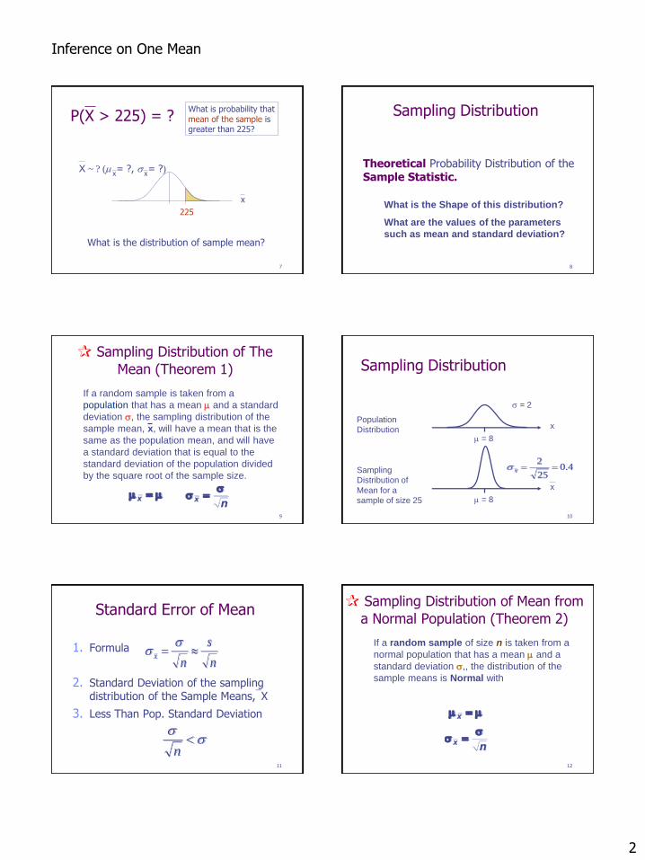
P(X > 225) = ?

225

x

X ~ ? (m = ?, s = ?)

What is probability that mean of the sample is greater than 225?

What is the distribution of sample mean?

x x

8

Theoretical Probability Distribution of the Sample Statistic.

Sampling Distribution

What is the Shape of this distribution?

What are the values of the parameters

such as mean and standard deviation?

9

Sampling Distribution of The

Mean (Theorem 1)

If a random sample is taken from a

population that has a mean m and a standard

deviation s, the sampling distribution of the

sample mean, x, will have a mean that is the

same as the population mean, and will have

a standard deviation that is equal to the

standard deviation of the population divided

by the square root of the sample size.

ss

xn

m mx

10


s = 2

m = 8

x Population

Distribution

m = 8

x

4.025

2xsSampling

Distribution of

Mean for a

sample of size 25

11

Standard Error of Mean

1. Formula

2. Standard Deviation of the sampling distribution of the Sample Means,X

3. Less Than Pop. Standard Deviation

n

s

nx

ss

ss

n

12

Sampling Distribution of Mean from

a Normal Population (Theorem 2)

If a random sample of size n is taken from a

normal population that has a mean m and a

standard deviation s,, the distribution of the

sample means is Normal with

ss

xn

m mx


3

13

Central Limit Theorem

(Theorem 3)

If a relative large random sample is taken

from a population that has a mean m and a

standard deviation s, regardless of the

distribution of the population, the

distribution of the sample means is

approximately normal with

ss

xn

m mx

14

A Random Sample from Population

Random Sample of Size 400 from Population

110.0

100.090.0

80.070.0

60.050.0

40.030.0

20.010.0

0.0

120

100

80

60

40

20

0

Std. Dev = 12.92

Mean = 20.7

N = 400.00

Population mean = 19.9, standard deviation = 12.6

15

Simulated Sampling Distribution of Means

SIZE2

77.073.0

69.065.0

61.057.0

53.049.0

45.041.0

37.033.0

29.025.0

21.017.0

13.09.0

5.01.0

70

60

50

40

30

20

10

0

Std. Dev = 8.88

Mean = 20.3

N = 400.00

n = 2 SIZE4

77.073.0

69.065.0

61.057.0

53.049.0

45.041.0

37.033.0

29.025.0

21.017.0

13.09.0

5.01.0

70

60

50

40

30

20

10

0

Std. Dev = 5.40

Mean = 19.4

N = 400.00

n = 4 SIZE10

77.073.0

69.065.0

61.057.0

53.049.0

45.041.0

37.033.0

29.025.0

21.017.0

13.09.0

5.01.0

100

80

60

40

20

0

Std. Dev = 4.32

Mean = 19.9

N = 400.00

n = 10

SIZE25

77.00

73.00

69.00

65.00

61.00

57.00

53.00

49.00

45.00

41.00

37.00

33.00

29.00

25.00

21.00

17.00

13.009.00

5.001.00

200

100

0

Std. Dev = 2.23

Mean = 19.84

N = 400.00

n = 25 SIZE50

77.00

73.00

69.00

65.00

61.00

57.00

53.00

49.00

45.00

41.00

37.00

33.00

29.00

25.00

21.00

17.00

13.009.00

5.001.00

200

100

0

Std. Dev = 1.64

Mean = 19.75

N = 400.00

n = 50 SIZE100

77.00

73.00

69.00

65.00

61.00

57.00

53.00

49.00

45.00

41.00

37.00

33.00

29.00

25.00

21.00

17.00

13.009.00

5.001.00

300

200

100

0

Std. Dev = 1.20

Mean = 19.81

N = 400.00

n = 100

16

Central Limit Theorem





of 46 mg/100 ml. If a random sample of

100 individuals is taken from the population,

what is the probability that the average

serum cholesterol level of these 100

individuals is higher than 225?

17

P(X > 225) = ?

225

0

z

3.04

225 - 211

4.6 = 3.04

.9988

1 - .9988 = .0012

x x

211

X ~ N (m = 211, s = 4.6)

n = 100

x

Cholesterol Level has a mean 211, s.d. 46.

By Central Limit Theorem

18

Estimation with Confidence Intervals

Confidence Intervals and

Sample Size


4

19

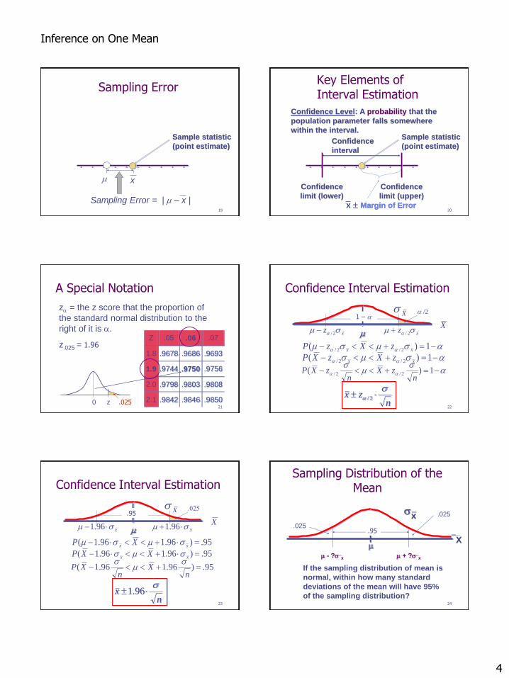
Sampling Error

Sample statistic

(point estimate)

x m

Sampling Error = | m – x | 20

Key Elements of Interval Estimation

Confidence

interval

Sample statistic

(point estimate)

Confidence

limit (lower)

Confidence

limit (upper)

x Margin of Error

Confidence Level: A probability that the

population parameter falls somewhere

within the interval.

x Margin of Error

21

A Special Notation

Z .05 .06 .07

1.8 .9678 .9686 .9693

1.9 .9744 .9750 .9756

2.0 .9798 .9803 .9808

2.1 .9842 .9846 .9850

z = the z score that the proportion of

the standard normal distribution to the

right of it is .

z.025 = ?

0 z .025

1.96

22

Confidence Interval Estimation

X

Xs

s

ms

-- 1)( 2/2/n

zXn

zXP

smsm -- 1)( 2/2/ xx zXzP

m

sms -- 1)( 2/2/ xx zXzXP

2/n

zxs

xz sm 2/xz sm 2/-

/2 1 –

23

Confidence Interval Estimation

X

Xs

95.)96.196.1( -n

Xn

XPs

ms

95.)96.196.1( - xx XP smsm

m

95.)96.196.1( - xx XXP sms

96.1n

xs

xsm 96.1xsm - 96.1

.025 .95

24

Sampling Distribution of the Mean

s x _

X m

If the sampling distribution of mean is

normal, within how many standard

deviations of the mean will have 95%

of the sampling distribution?

m - ?sx m + ?sx

.025

.025 .95


5

25

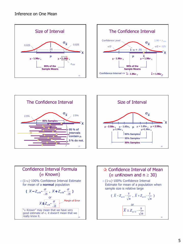
Size of Interval

s x _

X

m + 1.96sx m - 1.96sx

m

0.025 0.025

95% of the

Sample Means

z.025

.95

26

The Confidence Interval

s x _

X

m + 1.96sx m - 1.96sx

m

x + 1.96sx

x

Confidence Interval =>

1- = .95

Confidence Level

/2 /2 = .025

1.96 = z.025

x - 1.96sx

95% of the

Sample Means

27

95% Samples

s x _

X m

2.5% 2.5%

95 % of

intervals

contain m.

5 % do not.

The Confidence Interval

28

90% Samples

95% Samples

99% Samples

m + 1.65s x m + 2.58sx

s x _

X

m+1.96s x

m - 2.58s x m - 1.65sx

m-1.96s x

m

Size of Interval

29

(1-)·100% Confidence Interval Estimate

for mean of a normal population

or

) , ( 2/2/n

ZXn

ZXss

-

2/n

ZXs

Margin of Error

Confidence Interval Formula (s Known)

“s Known” may mean that we have very good estimate of s, it doesn’t mean that we really know it.

30

Confidence Interval of Mean (s unKnown and n 30)

(1-)·100% Confidence Interval

Estimate for mean of a population when sample size is relative large

or

),( 2/2/ n

sZX

n

sZX -

n

sZX 2/


6

31

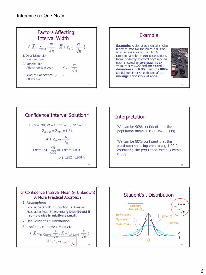
Factors Affecting Interval Width

1. Data Dispersion Measured by s

2. Sample Size Affects standard error

3. Level of Confidence (1 - ) Affects Z/2

n

x

ss

) ( 22n

zX,n

zX //

ss -

32

Example

Example: A city uses a certain noise index to monitor the noise pollution at a certain area of the city. A random sample of 100 observations from randomly selected days around noon showed an average index value of x = 1.99 and standard deviation s = 0.05. Find the 90% confidence interval estimate of the average noise index at noon.

33

Confidence Interval Solution*

) 998.1 , 982.1 (

0.008 1.99 100

05.64.199.1

1.64 ZZ

.05 /2 .1, 90.1 .90, 1

2/

.052 /

n

sZX

--

34

Interpretation

We can be 90% confident that the population mean is in (1.982, 1.998).

We can be 90% confident that the maximum sampling error using 1.99 for estimating the population mean is within 0.008.

35

Confidence Interval Mean (s Unknown) A More Practical Approach

1. Assumptions

Population Standard Deviation Is Unknown

Population Must Be Normally Distributed if sample size is relatively small.

2. Use Student’s t Distribution

3. Confidence Interval Estimate

) , ( 1,2/1,2/n

stX

n

stX nn - --

n

stX n -1 ,2/

36

t

Student’s t Distribution

0

t (df = 5)

Z

Standard

Normal (Z)

Bell-Shaped

Symmetric

‘Fatter’ Tails

t (df = 13)

ns

xt

m-


7

37

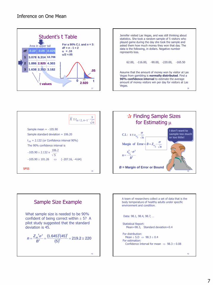
t0

Student’s t Table

2.920

.05

t values

For a 90% C.I. and n = 3:

df = n - 1 = 2

= .10

/2 =.05

df 0.10 0.05 0.025

1 3.078 6.314 12.706

2 1.886 2.920 4.303

3 1.638 2.353 3.182

Area in upper tail

38

Jennifer visited Las Vegas, and was still thinking about statistics. She took a random sample of 5 visitors who played game during the day she took the sample and asked them how much money they won that day. The data is the following, in dollars. Negative number represents loss.

62.00, -116.00, -90.00, -220.00, -165.50

Assume that the amount of money won by visitor at Las Vegas from gambling is normally distributed. Find a 90% confidence interval to estimate the average amount of money visitors win per day for visitors at Las Vegas.

39

Sample mean = -105.90

Sample standard deviation = 106.20

t.05 = 2.132 (or Confidence interval 90%)

The 90% confidence interval is

-105.90 2.132 x 106.2

5

(-207.16, -4.64) -105.90 101.26

SPSS

n

stX n -1 ,2/

40

Finding Sample Sizes for Estimating m

I don’t want to

sample too much

or too little!

2

22

2

2

2

Error ofMargin

nzx :C.I.

B

zn

nZB

s

s

s

B = Margin of Error or Bound

41

Sample Size Example

What sample size is needed to be 90% confident of being correct within 5? A

pilot study suggested that the standard deviation is 45.

2202.2195

45645.12

22

2

22

05. B

Zn

s

42

A team of researchers collect a set of data that is the body temperature of healthy adults under specific environment and condition.

Data: 98.1, 98.4, 98.7, …

Statistical Report: Mean=98.3, Standard deviation=0.4 For distribution: Mean S.D 98.3 0.4 For estimation: Confidence Interval for mean 98.3 0.08


8

43

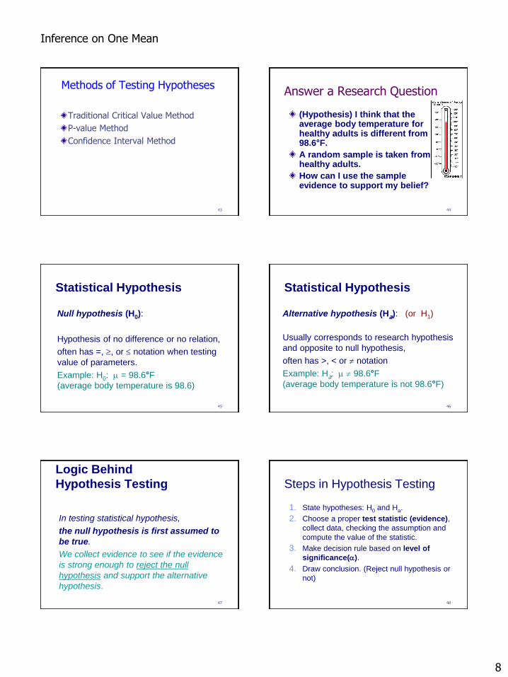
Methods of Testing Hypotheses

Traditional Critical Value Method

P-value Method

Confidence Interval Method

44

Answer a Research Question

(Hypothesis) I think that the average body temperature for healthy adults is different from 98.6°F.

A random sample is taken from healthy adults.

How can I use the sample evidence to support my belief?

45

Statistical Hypothesis

Null hypothesis (H0):

Hypothesis of no difference or no relation,

often has =, , or notation when testing

value of parameters.

Example: H0: m = 98.6°F (average body temperature is 98.6)

46

Statistical Hypothesis

Alternative hypothesis (Ha): (or H1)

Usually corresponds to research hypothesis

and opposite to null hypothesis,

often has >, < or notation

Example: Ha: m 98.6°F

(average body temperature is not 98.6°F)

47

Logic Behind

Hypothesis Testing

In testing statistical hypothesis,

the null hypothesis is first assumed to

be true.

We collect evidence to see if the evidence

is strong enough to reject the null

hypothesis and support the alternative

hypothesis.

48

Steps in Hypothesis Testing

1. State hypotheses: H0 and Ha.

2. Choose a proper test statistic (evidence),

collect data, checking the assumption and

compute the value of the statistic.

3. Make decision rule based on level of

significance().

4. Draw conclusion. (Reject null hypothesis or

not)


9

49

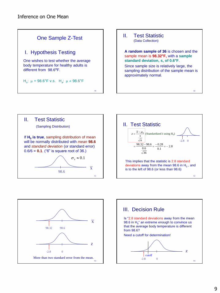
I. Hypothesis Testing

One wishes to test whether the average

body temperature for healthy adults is

different from 98.6°F.

Ho: m = 98.6°F v.s. Ha: m 98.6°F

One Sample Z-Test

50

A random sample of 36 is chosen and the

sample mean is 98.32°F, with a sample

standard deviation, s, of 0.6°F.

Since sample size is relatively large, the

sampling distribution of the sample mean is

approximately normal.

II. Test Statistic (Data Collection)

51

If H0 is true, sampling distribution of mean

will be normally distributed with mean 98.6

and standard deviation (or standard error)

0.6/6 = 0.1. (“6” is square root of 36.)

II. Test Statistic

(Sampling Distribution)

98.6 X

1.0xs

52

This implies that the statistic is 2.8 standard

deviations away from the mean 98.6 in H0 , and

is to the left of 98.6 (or less than 98.6)

8.2 1.0

28.0

36

6.0

6.9832.98

0

--

-

-

n

s

xz

m

II. Test Statistic

-2.8 0

(Standardized x using H0)

53

-2.8 0

Z

98.32 98.6

X

More than two standard error from the mean. 54

III. Decision Rule

Is “2.8 standard deviations away from the mean

98.6 in H0“ an extreme enough to convince us

that the average body temperature is different

from 98.6?

Need a cutoff for determination!

-2.8 0

Z

cutoff


10

55

Level of Significance

Level of significance for the test ()

A probability level selected by the

researcher at the beginning of the

analysis that defines unlikely values of

sample statistic if null hypothesis is true.

Total tail area =

c.v. 0 c.v.

c.v. = critical value

56

III. Decision Rule Critical value approach: Compare the test

statistic with the critical values defined by

significance level , usually = 0.05.

We reject the null hypothesis, if the test statistic

z < –z/2 = –z0.025 = –1.96, or

z > z/2 = z0.025 = 1.96.

–2.8

–1.96 0 1.96 Z

/2=0.025 /2=0.025

57





z < –z/2 = –z0.025 = –1.96, or

z > z/2 = z0.025 = 1.96.

Z

–2.8

–1.96 0 1.96

Critical values

Rejection

region Rejection

region

Two-sided Test

58

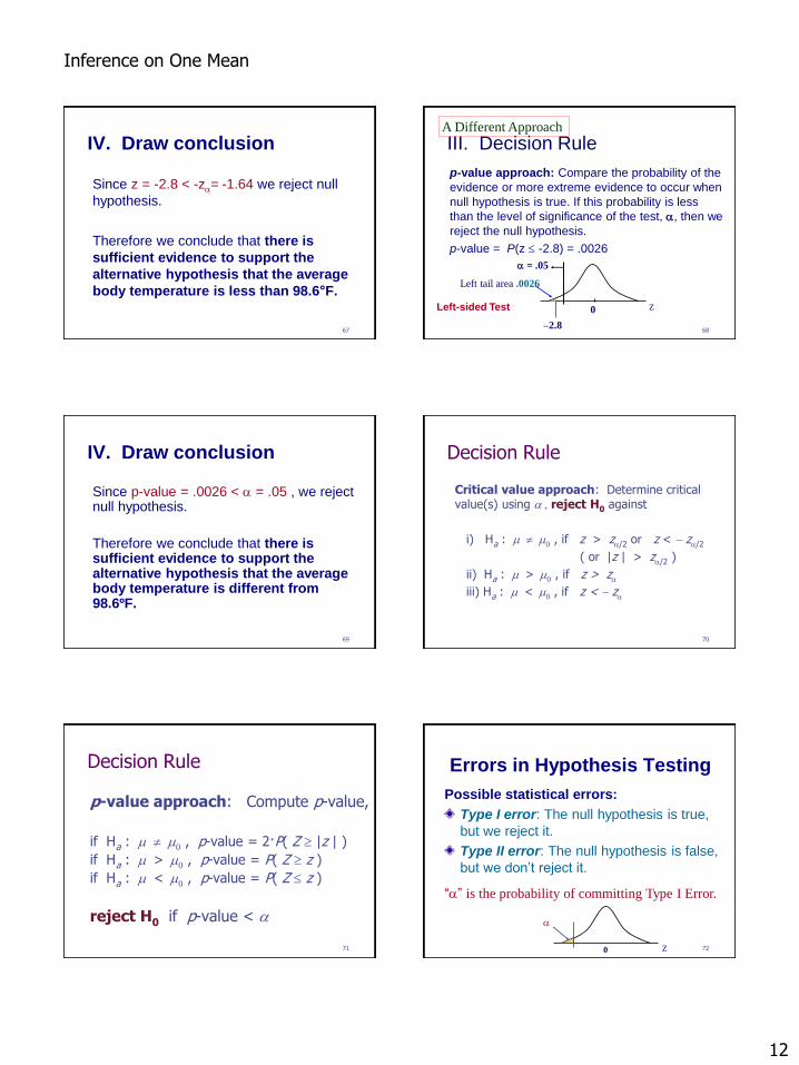
IV. Draw conclusion

Since z = -2.8 < -z/2= -1.96 therefore we reject null hypothesis.

Therefore we conclude that there is sufficient evidence to support the alternative hypothesis that the average body temperature is different from 98.6ºF.

59

III. Decision Rule

p-value approach: Compare the probability of the evidence or more extreme evidence to occur when null hypothesis is true. If this probability is less than the level of significance of the test, , then we reject the null hypothesis.

p-value = P(Z -2.8 or Z 2.8) = 2 x P(Z -2.8) = 2 x .0026 = .0052

Z

–2.8 2.8 0

Left tail area .003

Two-sided Test

A Different Approach

60

p-value

p-value (most popular approach)

The probability of obtaining a test statistic

that is as extreme or more extreme than

actual sample statistic value observed given

null hypothesis is true.

The smaller the p-value, the stronger the

evidence for supporting Ha and rejecting H0 .


11

61

IV. Draw conclusion

Since p-value = .0052 < = .05 , we reject null hypothesis.


62

I. Hypothesis Testing

One wishes to test whether the average

body temperature for healthy adults is

less than 98.6°F.

Ho: m = 98.6°F v.s. Ha: m < 98.6°F

This is a one-sided test, left-side test.

63

A random sample of 36 is chosen and the

sample mean is 98.32°F, with a sample

standard deviation, s, of 0.6°F.

Assumption: Assume body temperature for

healthy adults under regular environment

has a normal distribution.

II. Test Statistic

64

If H0 is true, sampling distribution of mean

will be normally distributed with mean 98.6

and the estimated standard deviation (or

standard error) 0.6/6 = 0.1. (“6” is square

root of 36.)

II. Test Statistic

98.6 X

65

This implies that the statistic is 2.8 standard

deviations away from the mean 98.6 in H0 , and

is to the left of 98.6 (or less than 98.6)

8.2 1.0

28.0

36

6.0

6.9832.98

0

--

-

-

n

s

xz

m

II. Test Statistic

-2.8 0

66





z < –z = –z0.05 = –1.64.

Z

=0.05

–2.8

–1.64 0

Critical values

Rejection

region

Left-sided Test


12

67

IV. Draw conclusion

Since z = -2.8 < -z= -1.64 we reject null

hypothesis.

Therefore we conclude that there is

sufficient evidence to support the

alternative hypothesis that the average

body temperature is less than 98.6°F.

68

III. Decision Rule

p-value approach: Compare the probability of the

evidence or more extreme evidence to occur when

null hypothesis is true. If this probability is less

than the level of significance of the test, , then we

reject the null hypothesis.

p-value = P(z -2.8) = .0026

Z

–2.8

0

Left tail area .0026

Left-sided Test

= .05

A Different Approach

69

IV. Draw conclusion

Since p-value = .0026 < = .05 , we reject null hypothesis.


70

Decision Rule

Critical value approach: Determine critical value(s) using , reject H0 against

i) Ha : m m0 , if z > z/2 or z < - z/2

( or |z | > z/2 )

ii) Ha : m > m0 , if z > z

iii) Ha : m < m0 , if z < - z

71

Decision Rule

p-value approach: Compute p-value,

if Ha : m m0 , p-value = 2·P( Z |z | )

if Ha : m > m0 , p-value = P( Z z )

if Ha : m < m0 , p-value = P( Z z )

reject H0 if p-value <

72

Errors in Hypothesis Testing

Possible statistical errors:

Type I error: The null hypothesis is true,

but we reject it.

Type II error: The null hypothesis is false,

but we don’t reject it.

Z 0

“” is the probability of committing Type I Error.


13

73

Can we see data and then

make hypothesis?

1. Choose a test statistic, collect data, checking the assumption and compute the value of the statistic.

2. State hypotheses: H0 and Ha.

3. Make decision rule based on level of significance().

4. Draw conclusion. (Reject null hypothesis or not)

74

• Statistical Significance • Practical Significance

m < 70

m < 65 = 70 – 5

Significance of Effect

75

One-sample t-Test

(with Unknown Variance s 2)

In practice, population variance is unknown

most of the time. The sample standard

deviation s2 is used instead for s2. If the

random sample of size n is from a normal

distributed population and if the null hypothesis

is true, the test statistic (standardized sample

mean) will have a t-distribution with degrees of

freedom n-1.

n

s

xt 0 :StatisticTest

m-

76

I. State Hypothesis

One-side test example:

If one wish to test whether the body

temperature is less than 98.6 or not.

H0: m = 98.6 v.s. Ha: m < 98.6

(Left-sided Test)

77

II. Test Statistic

If we have a random sample of size 16 from a normal population that has a mean of 98.32°F, and a sample standard deviation 0.4. The test statistic will be a t-test statistic and the value will be: (standardized score of sample mean)

Under null hypothesis, this t-statistic has a t-distribution with degrees of freedom n – 1, that is, 15 = 16 - 1.

8210

280

16

40

69832980 . .

.

.

.. :StatisticTest -

-

-

-

n

s

xt

m

78

III. Decision Rule

Critical Value Approach:

To test the hypothesis at level 0.05,

the critical value is –t = –t0.05 = –1.753.

t –1.753

Rejection

Region

0

Descion Rule: Reject null hypothesis if t < –1.753


14

79

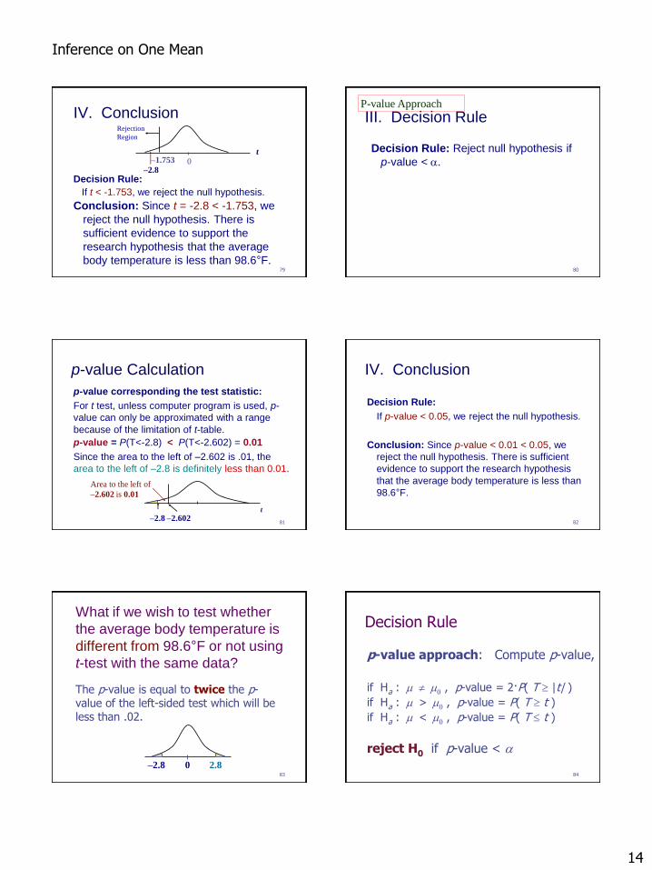
IV. Conclusion

Conclusion: Since t = -2.8 < -1.753, we

reject the null hypothesis. There is

sufficient evidence to support the

research hypothesis that the average

body temperature is less than 98.6°F.

–2.8

t

0 –1.753

Rejection

Region

Decision Rule:

If t < -1.753, we reject the null hypothesis.

80

III. Decision Rule

Decision Rule: Reject null hypothesis if

p-value < .

P-value Approach

81

p-value Calculation

p-value corresponding the test statistic:

For t test, unless computer program is used, p-

value can only be approximated with a range

because of the limitation of t-table.

p-value = P(T<-2.8) = ?

t

–2.8 –2.602

Area to the left of

–2.602 is 0.01

p-value = P(T<-2.8) < P(T<-2.602) = 0.01

Since the area to the left of –2.602 is .01, the

area to the left of –2.8 is definitely less than 0.01.

82

IV. Conclusion

Decision Rule:

If p-value < 0.05, we reject the null hypothesis.

Conclusion: Since p-value < 0.01 < 0.05, we

reject the null hypothesis. There is sufficient

evidence to support the research hypothesis

that the average body temperature is less than

98.6°F.

83

What if we wish to test whether

the average body temperature is

different from 98.6°F or not using

t-test with the same data?

The p-value is equal to twice the p-value of the left-sided test which will be less than .02.

–2.8 0 2.8 84

Decision Rule

p-value approach: Compute p-value,

if Ha : m m0 , p-value = 2·P( T |t| )

if Ha : m > m0 , p-value = P( T t )

if Ha : m < m0 , p-value = P( T t )

reject H0 if p-value <


15

85

Decision Rule

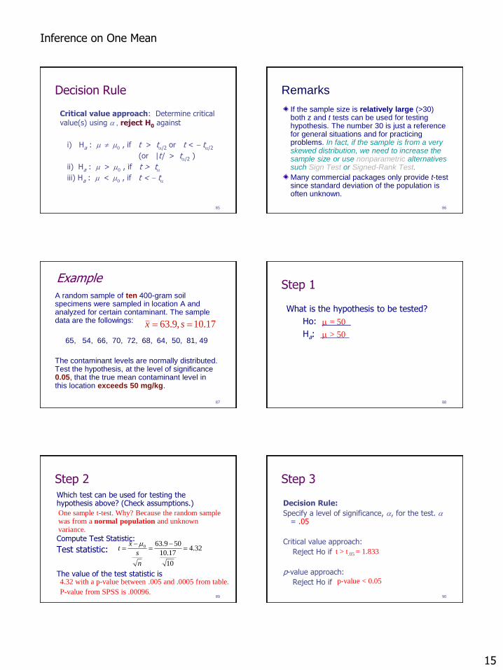
Critical value approach: Determine critical value(s) using , reject H0 against

i) Ha : m m0 , if t > t/2 or t < - t/2

(or |t| > t/2 )

ii) Ha : m > m0 , if t > t

iii) Ha : m < m0 , if t < - t

86

Remarks

If the sample size is relatively large (>30) both z and t tests can be used for testing hypothesis. The number 30 is just a reference for general situations and for practicing problems. In fact, if the sample is from a very skewed distribution, we need to increase the sample size or use nonparametric alternatives such Sign Test or Signed-Rank Test.

Many commercial packages only provide t-test since standard deviation of the population is often unknown.

87

Example

A random sample of ten 400-gram soil specimens were sampled in location A and analyzed for certain contaminant. The sample data are the followings:

65, 54, 66, 70, 72, 68, 64, 50, 81, 49

The contaminant levels are normally distributed. Test the hypothesis, at the level of significance 0.05, that the true mean contaminant level in this location exceeds 50 mg/kg.

17.10,9.63 sx

88

Step 1

What is the hypothesis to be tested?

Ho: ______

Ha: ______

m = 50

m > 50

89

Step 2 Which test can be used for testing the hypothesis above? (Check assumptions.)

Compute Test Statistic:

Test statistic:

The value of the test statistic is

32.4

10

17.10

509.63 0

-

-

n

s

xt

m

One sample t-test. Why? Because the random sample was from a normal population and unknown variance.

4.32 with a p-value between .005 and .0005 from table.

P-value from SPSS is .00096. 90

Step 3

Decision Rule:

Specify a level of significance, , for the test. = .05

Critical value approach:

Reject Ho if

p-value approach:

Reject Ho if

t > t.05 = 1.833

p-value < 0.05


16

91

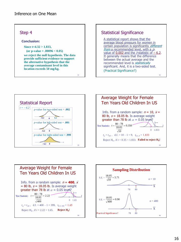
Step 4

Conclusion:

Since t=4.32 > 1.833,

(or p-value = .00096 < 0.05)

we reject the null hypothesis. The data provide sufficient evidence to support the alternative hypothesis that the average contaminant level in this location exceeds 50 mg/kg.

92

Statistical Significance

A statistical report shows that the average blood pressure for women in certain population is significantly different from a recommended level, with a p-value of 0.002 and the t-statistic of – 6.2. It generally means that the difference between the actual average and the recommended level is statistically significant. And, it is a two-sided test.

(Practical Significance?)

93

Statistical Report

p-value for two-sided test = .002

–6.2 6.2 0

t = - 6.2

p-value for left-sided test = .001

–6.2 0

p-value for right-sided test = .999

– 6.2 0 94

Average Weight for Female Ten Years Old Children In US

Info. from a random sample: n = 10, x = 80 lb, s = 18.05 lb. Is average weight greater than 78 lb at = 0.05 level?

t = t.05 , d.f. = 10 – 1 = 9, t0.5, 9 = 1.833

Reject H0 , if t = 0.35 < 1.833. Failed to reject H0!

350.0

10

05.18

7880

-tTest Statistic:

0 1.833

t

95

Average Weight for Female Ten Years Old Children In US

Info. from a random sample: n = 400, x = 80 lb, s = 18.05 lb. Is average weight greater than 78 lb at = 0.05 level?

t = t.05 , d.f. = 400 – 1 = 399, t0.5, 399 = 1.65

Reject H0 , if t = 2.22 > 1.65. Reject H0!

22.2

400

05.18

7880

-tTest Statistic:

0 1.65

t

96

78 80

X

n = 10 71.5

10

05.18S.E. =

78 80

X

n = 400 90.0

400

05.18S.E. =


Practical Significance?

Latest Cholesterol Levels Standards A Normal...

Documents

Transcript of Latest Cholesterol Levels Standards A Normal...