LATERAL LOAD DISTRIBUTION FOR STEEL BEAMS SUPPORTING AN FRP PANEL

by

HARRISON WALKER POOLE

B.S., Kansas State University, 2009

A THESIS

submitted in partial fulfillment of the requirements for the degree

MASTER OF SCIENCE

Civil Engineering

College of Engineering

KANSAS STATE UNIVERSITY

Manhattan, Kansas

2011

Approved by:

Major Professor

Dr. Hani Melhem

Copyright

HARRISON POOLE

2011

Abstract

Fiber Reinforced Polymer (FRP) is a relatively new material used in the field of civil

engineering. FRP is composed of fibers, usually carbon or glass, bonded together using a

polymer adhesive and formed into the desired structural shape. Recently, FRP deck panels have

been viewed as an attractive alternative to concrete decks when replacing deteriorated bridges.

The main advantages of an FRP deck are its weight (roughly 75% lighter than concrete), its high

strength-to-weight ratio, and its resistance to deterioration. In bridge design, AASHTO provides

load distributions to be used when determining how much load a longitudinal beam supporting a

bridge deck should be designed to hold. Depending on the deck material along with other

variables, a different design distribution will be used. Since FRP is a relatively new material

used for bridge design, there are no provisions in the AASHTO code that provides a load

distribution when designing beams supporting an FRP deck. FRP deck panels, measuring 6 ft x

8.5’, were loaded and analyzed at KSU over the past 4 years. The research conducted provides

insight towards a conservative load distribution to assist engineers in future bridge designs with

FRP decks.

Two separate test periods produced data for this thesis. For the first test period,

throughout the year of 2007, a continuous FRP panel was set up at the Civil Infrastructure

Systems Laboratory at Kansas State University. This continuous panel measured 8.5 ft by 6 ft x

6 in. thick and was supported by 4 Grade A572 HP 10 x 42 steel beams. The beam spacing’s,

along the 8.5 ft direction, were 2.5 ft-3.5 ft-2.5 ft. Stain gauges were mounted at mid-span of

each beam to monitor the amount of load each beam was taking under a certain load. Linear

variable distribution transformers (LVDT) were mounted at mid-span of each beam to measure

deflection. Loads were placed at the center of the panel, with reference to the 6 ft direction and

at several locations along the 8.5 ft direction. Strain and deflection readings were taken in order

to determine the amount of load each beam resisted for each load location.

The second period of testing started in the fall of 2010 and extended into January of

2011. This consisted of a simple-span/cantilever test set-up. The test set-up consisted of, in the

8.5 ft direction, a simply supported span of 6 ft with a 2.5 ft cantilever on one side. As done

previously both beams had strain gauges along with LVDTs mounted at mid-span. There were

also strain gauges were installed spaced at 1.5ft increments along one beam in order to analyze

the beam behavior under certain loads. Loads were once again applied in the center of the 6 ft

direction and strain and deflection readings were taken at several load locations along the 8.5 ft

direction. The data was analyzed after all testing was completed. The readings from the strain

gauges mounted in 1.5 ft increments along the steel beam on one side of the simple span test set-

up were used to produce moment curves for the steel beam at various load locations. These

moment curves were analyzed to determine how much of the panel was effectively acting on the

beam when loads were placed at various distances away from the beam. Using these “effective

lengths,” along with the strain taken from the mid-span of each beam, the loads each beam was

resisting for different load locations were determined for both the continuously supported panel

and the simply supported/cantilever panel data. Using these loads, conservative design factors

were determined for FRP panels. These factors are S/5.05 for the simply supported panel and

S/4.4 for the continuous panel, where “S” is the support beam spacing. Deflections

measurements were used to validate the results. Percent errors, based on experimental and

theoretical deflections, were found to be in the range of 10 percent to 40 percent depending on

the load locations for the results in this thesis.

v

Table of Contents

List of Figures .............................................................................................................................. viii

List of Tables ................................................................................................................................. xi

Acknowledgements ...................................................................................................................... xiii

CHAPTER 1 - Introduction and Literature Review ....................................................................... 1

1.1 Introduction ........................................................................................................................... 1

1.2 Literature Review ................................................................................................................. 2

1.2.1 Kumar, Chandrashekhara, and Nanni ............................................................................ 2

1.2.2 Temeles .......................................................................................................................... 3

1.2.3 Allampalli & Kunn ........................................................................................................ 5

1.2.4 Bakis et al. ...................................................................................................................... 6

1.2.5 Hayes et al. ..................................................................................................................... 7

1.2.6 Kalny .............................................................................................................................. 7

1.2.7 Plunkett ........................................................................................................................ 10

1.2.8 Schreiner ...................................................................................................................... 11

CHAPTER 2 - Material Properties, Testing Program, and Data Analysis ................................... 12

2.1 Material Properties .............................................................................................................. 12

2.1.1 FRP Panel ..................................................................................................................... 13

2.1.2 Steel Beams and Rigid Frame ...................................................................................... 14

2.2 Testing Configuration ......................................................................................................... 15

2.2.1 Continuous Panel ......................................................................................................... 15

2.2.1.1 Continuous Panel Instrumentation ........................................................................ 18

2.2.2 Simple/Cantilever Panel ............................................................................................... 20

2.2.2.1 Simple Span/Cantilever Panel Instrumentation .................................................... 22

2.3 Testing Procedure ............................................................................................................... 23

2.3.1 Simple Span/Cantilever ............................................................................................... 23

2.3.2 Continuous Panel ......................................................................................................... 23

2.4 Data Analysis ...................................................................................................................... 24

CHAPTER 3 - Load Distribution on Steel Beams........................................................................ 25

vi

3.1 Determining Moments ........................................................................................................ 25

3.2 Analyzing Moments ............................................................................................................ 26

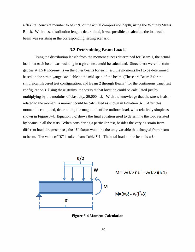
3.3 Determining Beam Loads ................................................................................................... 30

CHAPTER 4 - Simple Span/Cantilever Testing ........................................................................... 32

4.1 Distribution Lengths and Determining Loads .................................................................... 32

4.2 Simple Span Load Distribution ........................................................................................... 34

4.3 Cantilever Analysis ............................................................................................................. 37

4.4 LVDT Results – Simple Span/Cantilever ........................................................................... 39

CHAPTER 5 - Continuous Panel Testing ..................................................................................... 42

5.1 Load Distribution on Beams ............................................................................................... 42

5.2 Continuous Panel Analysis ................................................................................................. 42

CHAPTER 6 - Panel Strain Analysis............................................................................................ 49

6.1 Tongue Edge – Center of Beam 2 ....................................................................................... 49

6.2 Tongue Edge – MS 2-3 ....................................................................................................... 51

CHAPTER 7 - Conclusions .......................................................................................................... 52

CHAPTER 8 - Bibliography ......................................................................................................... 55

Appendix A - Test Set-Up ............................................................................................................ 56

A- 1 Continuous Panel ........................................................................................................... 57

A-2 Simple Span/Cantilever Set-Up ................................................................................. 58

A-3 Cross Sections and Details ................................................................................................ 59

Appendix B - Moment Curves/Distribution Lengths.................................................................... 62

B-1 Moments ............................................................................................................................ 63

B-2 Lengths of Uniform Load .................................................................................................. 65

Appendix C - Simple Span/Cantilever Test Results ..................................................................... 66

C-1 Loading Scenario: CL BM 1 .............................................................................................. 67

C-2 Loading Scenario: 1.25’ OC BM1 ..................................................................................... 70

C-3 Loading Scenario: Center of SS ......................................................................................... 73

C-4 Loading Scenario: OPP BM .............................................................................................. 76

C-5 Loading Scenario: CNTLVR ............................................................................................. 79

C-6 Load Ratio Charts .............................................................................................................. 82

C-7 Load Ratio Summary ......................................................................................................... 83

vii

Appendix D - Continuous Panel Test Results............................................................................... 84

D-1 Loading Scenario: CL BM1 .............................................................................................. 85

D-2 Loading Scenario: MS 1-2 ................................................................................................ 88

D-3 Loading Scenario: CL BM2 .............................................................................................. 91

D-4 Loading Scenario: MS 2-3 ................................................................................................. 94

D-5 Loading Scenario: CL BM 3 ............................................................................................. 97

D-6 Load Ratios – Cont. Test ................................................................................................. 100

D-7 Load Distribution Summary ............................................................................................ 104

viii

List of Figures

Figure 2-1 Tongue and Groove Connection (Left) & Tongue Edge (Right) ................................ 12

Figure 2-2 Face Lay-up Schedule ................................................................................................. 13

Figure 2-3 Continuous Panel Test Configuration ......................................................................... 16

Figure 2-4 Panel Connection Detail .............................................................................................. 17

Figure 2-5 (a) Actuator Used to Load Panel (b) Foot with Rubber Pad ....................................... 18

Figure 2-6 Picture of (a) Metal C Shape (b) LVDT (c) Optim Megadac 200 .............................. 19

Figure 2-7 Continuous Panel Instrumentation .............................................................................. 20

Figure 2-8 Simple Span/Cantilever Test Configuration ............................................................... 21

Figure 2-9 Simple Span/Cantilever Instrumentation .................................................................... 22

Figure 3-1 Beam 1 Moment Curve at Load Magnitude of 15 kips ............................................... 27

Figure 3-2 Shear, Moment, Deflection Diagram for Uniform Load Partially Distributed (AISC,

2008) ..................................................................................................................................... 28

Figure 3-3 Beam 1 Analyzed Moment Curves at Load Magnitude of 15 kips (Additional

Figures B-2 and B-3 contain moments curves at different load magnitudes) ....................... 28

Figure 3-4 Moment Calculation .................................................................................................... 30

Figure 4-1 Load Ratio Graphs for a Load Magnitude of (a) 10 kips, (b) 15 kips, and ................ 35

Figure 4-2 Experimental vs. Theoretical Deflections – CL BM1 – Simple Span ........................ 41

Figure 5-1 Loading Scenario - Beam 1 - Load Magnitude: 20 kips…………………………..…43

Figure 5-2 Load Ratio for (a) Beam 1 and (b) Beam 4 for Load magnitude of 20 kips…………43

Figure 5-3 Loading Scenarios - Load Magnitude - 20 kips…………………//………………/…46

Figure 5-4 Load Ratios for (a) Beam 2 and (b) Beam 3 for Load Magnitude of 20 kips………..46

Figure 5-5 Deflections - CL BM1 - Cont. Test…………………………………………………..48

Figure 6-1 Panel Strain for Load at Tongue Edge above BM 2 at a Load Magnitude of 22 kips 49

Figure 6-2 Panel Strain for Load at Tongue Edge of MS 2-3 at a Load Magnitude of 22 kips ... 51

Figure A-1 Continuous Panel Test Set-Up ................................................................................... 57

Figure A-2 Cross Section of Continuous Panel Test - View Toward East ................................... 57

Figure A-3 Simple Span/Cantilever Test Set-Up.......................................................................... 58

Figure A-4 Cross Section of Simple Span/Cantilever Test - View Toward East ......................... 58

Figure A-5 Typ. Cross Section - View Toward North.................................................................. 59

ix

Figure A-6 Cross Section - Simple Span/Cantilever Test - View Toward North ......................... 59

Figure A-7 Connection Detail - FRP Deck to Steel Beam Connection ........................................ 60

Figure A-8 Strain Gauge Locations .............................................................................................. 60

Figure A-9 Example of Current AASHTO Load Distribution Factors......................................... 61

Figure A-10 AASHTO Truck Wheel Dimensions ........................................................................ 61

Figure B-1 Moment Curves for Load Magnitudes of (a) 10 kips, (b) 15 kips, and (c) 20 kips….64

Figure B-2 Length of Uniform Load…………………………………………………………….65

Figure C-1 Load Location - CL BM1……………………………………………………………67

Figure C-2 CL BM1 Test Picture………………………………………………………………...67

Figure C-3 Beam Reactions - CL BM1…………………………………………...……………..68

Figure C-4 Deflection - CL BM1……………………………………………………………….69

Figure C-5 Load Location - 1.25' OC BM1……………………………………………………..70

Figure C-6 1.25' OC BM1 Test Picture………………………………………………………….70

Figure C-7 Beam Reactions - 1.25' OC BM1……………………………………………………71

Figure C-8 Deflections - 1.25' OC BM1………………………………………………………....72

Figure C-9 Load Locations - Center of SS………………………………………………………73

Figure C-10 Center of SS Test Picture…………………………………………………………..73

Figure C-11 Beam Reactions - Center of SS……………………………………………………74

Figure C-12 Deflections - Center of SS…………………………………………………………76

Figure C-13 Load Location - OPP BM………………………………………………………….77

Figure C-14 OPP BM Test Picture……………………………………………………………...77

Figure C-15 Beam Reactions OPP BM…………………………………………………………78

Figure C-16 Deflections -OPP BM……………………………………………………………...79

Figure C-17 Load Locations - CNTLVR…………………………………………………….….80

Figure C-18 CNTLVR Test Picture…………………………………………………….………..80

Figure C-19 Beam Reactions - CNTLVR…………………………………………………….…81

Figure C-20 Deflections - CNTLVR…………………………………………………….………82

Figure C-21 Load Ratio Charts for Load Magnitudes of (a) 10 kips, (b) 15 kips, and (c) 20 kips-

Simple Span…………………………………………………………………………//….84

Figure D-1 Load Locations - CL BM1 - Cont. Test………………………………………..……85

Figure D-2 Reactions - CL BM1………………………………………..……………………….86

x

Figure D-3 Deflections - CL BM1……….………………………………………………………87

Figure D-4 Load Location 0 MS 1-2………………………………………………………...…..88

Figure D-5 Beam Reactions - MS 1-2…………………………………………………………...89

Figure D-6 Deflections - MS 1-2………………………………………………………………...90

Figure D-7 Load Locations - CL BM2 - Cont. Test……………………………………………..91

Figure D-8 Beam Reactions - CL BM2………………………………………………………….92

Figure D-9 Deflections - CL BM2………………………………………………………………93

Figure D-10 Load Locations - MS 2-3…………………………………………………………..94

Figure D-11 Beam Reactions - MS 2-3……………………………………….…………………95

Figure D-12 Deflections - MS 2-3……………………………………………………………….96

Figure D-13 Load Location - CL BM3……………………………….………………………….97

Figure D-14 Beam Reactions - CL BM3………………………………………………………..98

Figure D-15 Deflections - CL BM3……………………………………………………………..99

Figure D-16 Load Ratio Chart BM 1 for Load Magnitudes of (a) 10 kips, (b) 15 kips, and (c) 20

kips - Cont. Test………………………………………………………………………...100

Figure D-17 Load Ratio Chart BM 2 for Load Magnitudes of (a) 10 kips, (b) 15 kips, and (c) 20

kips - Cont. Test…………………………………………..……………………………103

Figure D-18 Load Ratio Chart BM 3 for Load Magnitudes of (a) 10 kips, (b) 15 kips, and (c) 20

kips - Cont. Test………………………………………………………………………..104

Figure D-19 Load Ratio Chart BM4 for Load Magnitudes of (a) 10 kips, (b) 15 kips, and (c) 20

kips - Cont. Test……………………………………………………………….………105

xi

List of Tables

Table 4-1 Simple Span Analysis .................................................... Error! Bookmark not defined.

Table 4-2 Simple Span Load Distribution .................................................................................... 37

Table 4-3 Cantilever Ratios .......................................................................................................... 38

Table 4-4 Experimental vs. Theoretical Deflections – CL BM1 – Simple Span .......................... 41

Table 5-1 Load Distribution Summary for Beam 1 ...................................................................... 45

Table 5-2 Load Distribution Summary for Beam 2 ...................................................................... 47

Table 5-3 Experimental vs. Theoretical Deflections - CL BM1 - Cont. Test ............................... 48

Table B-1 Moment Curve Data (kip*ft) ....................................................................................... 63

Table B-2 Load Distribution Lengths ........................................................................................... 65

Table C-1 Reactions - CL BM1………………………………………………………………….68

Table C-2 Experimental/Theoretical Deflections - CL BM1……………………………………69

Table C-3 Reactions -1.25' OC BM 1……………………………………………………….…...71

Table C-4 Experimental/Theoretical Deflections - 1.25' OC BM1………………………….….72

Table C-5 Reactions - Center of SS….……………………………………………….………….74

Table C-6 Experimental/Theoretical Deflections - Center of SS..………………………………75

Table C-7 Reactions -OPP BM………………………………………………..………………....77

Table C-8 Experimental/Theoretical Deflections - OPP BM…….……………………….…….78

Table C-9 Reactions - CNTLVR………………………………………………………………...80

Table C-10 Experimental/Theoretical Deflections - CNTLVR………………………….……....81

Table C-11 Load Ratio Analysis - Simple Span.……………………………………………..….83

Table D-1 Reactions - CL BM1………………………………………………………….……....86

Table D-2 Experimental/Theoretical Deflections - CL BM1……………….…………….……..87

Table D-3 Reactions - MS 1-2……………………………………………………………….…..89

Table D-4 Experimental/Theoretical Deflections - MS 1-2………………………………….….90

Table D-5 Reactions - CL BM2……………………………………………………………….....92

Table D-6 Experimental/Theoretical Deflections - CL BM2………………………………..…..93

Table D- 7 Reactions - MS 2-3……………………………………………………………..……95

Table D-8 Experimental/Theoretical Deflections - MS 23…………………………………...….96

Table D-9 Reactions - CL BM3…………………………………………………………….……98

xii

Table D-10 Experimental/Theoretical Deflections………………………………….…/………..99

Table D-11 Load Distribution Summary - BM 1 - Cont. Test………………………………….104

Table D-12 Load Distribution Summary - BM 2 - Cont. Test………………………………….105

Table D-13 Load Distribution Summary - BM 3 - Cont. Test………………………………….106

Table D-14 Load Distribution Summary - BM 4 - Cont. Test………………………………….107

xiii

Acknowledgements

The author would like to recognize the following people for their support and helpfulness

during the research detailed in this thesis:

Dr. Hani Melhem, for serving as my advisor and his constant guidance and help during

the data analysis. His deep background in structural engineering as well as mathematics was

extremely useful for analyzing the beam behavior as well as the panel behavior in this thesis. Dr.

Robert Peterman, for providing knowledge about the instrumentation and tools used for during

testing as well as serving on my committee. Dr. Asad Esmaeily, for serving on my committee.

Mr. Dave Meggers, from the Kansas Department of Transportation, for his continual guidance

during testing and his background knowledge on the subject of FRP. Dr. Moni El-Aasar for his

input on the research from a design perspective as well as his knowledge on FRP- bridge

components.

Thanks to the Kansas State University Transportation Center for financial support during

my graduate studies.

In conclusion, I would like to thank Mr. Kory Rankin and other structure Kansas State

graduate students for their help with testing and analysis of my research. My experience would

have been much more difficult without their help.

1

CHAPTER 1 - Introduction and Literature Review

1.1 Introduction

FRP is a composite material consisting of fibers made out of materials such as carbon or

glass, bonded together using an epoxy-polymer. Although FRP has been used for over half a

century in Aerospace Engineering applications, its use is generally new is other engineering

disciplines.

The most common form of FRP in Civil Engineering is found in pultruded shapes that

can be used as structural materials. More recently FRP honeycomb decks have been used to

replace existing deteriorated bridge decks. These new FRP decks have several advantages such

as a high strength to weight ratio, great weather resistance, and minimal construction time.

The high strength-to-weight ratio allows bridges to increase their load capacity since the

FRP will allow for additional live loads due to a reduction in dead loads. FRP is extremely

resilient against weather and will not deteriorate nearly as quick as other materials such as steel

in high sulfate environments. The time required to replace an existing bridge deck with an FRP

deck is very small, taking as little as a day, compared to the weeks it could take to replace an

existing bridge deck with a new concrete deck. Consequently, although FRP costs substantially

more than concrete, the reduced labor costs and time requirements more than compensate for the

additional material costs, translating into overall cost savings in bridge construction. States that

have implemented FRP include: Kansas, Missouri, West Virginia, New York, Colorado, Ohio,

Maryland, and Pennsylvania.

Due to the fact that it is not commonly used in construction, there are no design standards

or codes for designing bridge elements with FRP decks. Consequently, most designs using FRP

that have been implemented up to this point have used experimental data along with computer

modeling. The American Association of State Highway and Transportation Officials

(AASHTO) provides distribution factors for beams supporting bridge decks made from other

materials. These distribution factors are dependent on the spacing of the beams supporting the

bridge decks. There are also different factors for different bridge constructions. For example, a

bridge with a timber deck supported by steel beams will have a different factor than a bridge

with a concrete deck supported on steel beams. For ASD, these factors are in terms of the beam

spacing “S” divided by a certain variable dependent upon the situation. After substituting the

2

spacing, the resulting factor represents the load on the bridge deck for which that particular beam

needs to be designed for. For example, if there is a 10 kip wheel load on a bridge with a

longitudinal beam spacing of 4 ft and the AASHTO design factor for this particular bridge is S/8,

then that beam needs to be designed to support 4/8 or 0.5 of the wheel load, which equals 5 kips.

AASHTO provides these design factors for most common materials, however due to the limited

use of FRP, there are no stipulations for FRP in the specifications.

The main objective of the research detailed in this thesis is to determine a conservative

lateral load distribution factor for FRP that would assist design engineers. Data was collected

from two different testing periods, including the year of 2007, and also the fall of 2010 extending

into January of 2011. The original testing in 2007 consisted of a panel continuously supported

while the more recent tests were performed on a panel with a simple span/cantilever set-up. For

the original testing, strain gauges were placed at mid-span of the supporting beams to determine

the reactions along with LVDTs to measure beam deflections. The instrumentation was the same

in the simple span/cantilever testing, however strain gauges were added along one beam in order

to determine the behavior of the beam during various loading circumstances. After the reactions

were determined from all the data, distribution factors were established for the FRP panel

supported on steel beams by modeling different loading scenarios.

Strain gauges were also placed at 6 in. spacing along the panel in three rows. These

provided some insight into the behavior of the panel during loading. This data was not

completely necessary for determining distribution factors, however, it is briefly discussed in

Chapter 6. It can be found on the (Data CD) for further analysis.

1.2 Literature Review

1.2.1 Kumar, et al

Kumar, et al (Kumar, et al., March 2001) completed research on an FRP panel used in the

design of a bridge on the Missouri Rolla University Campus. The bridge design consisted of a

deck made out of hollow 3 in. square FRP pultruded tube shapes bonded together to form I-

shapes. Each I shape consisted of 7 layers of these square tubes alternately laid longitudinally

and transversely. The tubes were connected together using an epoxy adhesive. The flanges were

approximately 8 tubes across while the webs had a width of 4 tubes. Only one of the I shape

3

members were fabricated and used for experimental purposes. Experimental tests included a

design load test, a fatigue test, and an ultimate load test. The design load test proved that the

structure was capable of taking the AASHTO required design load measuring deflection along

with visual observations. It was found that the deflection was more than adequate for the

maximum design load. The fatigue testing included 2 million cycles where the structure was

continuously unloaded to 500 pounds and reloaded to 11,000 pounds. Every 400,000 cycles, the

test was paused and a static load was applied to check for any loss of stiffness in the member.

All results concluded that the member did not lose any stiffness due to fatigue. The ultimate load

test proved the structure to be able to withstand several times the required design load. The

failure observed was not violent and it was concluded that in the case of an actual bridge failure,

occupants would have sufficient time to evacuate the structure before collapse.

1.2.2 Temeles

Temeles (Temeles, 2001) developed a “testing facility” to analyze the performance of

two FRP decks. The testing facility consisted of a bay cut out of the concrete road leading up to

a weigh station on Interstate 81 in Virginia. A FRP panel would be laid in the bay in order to

monitor the strains and deflections over an extended period of time as trucks passed over. Upon

fabrication of the first panel, some design deficiencies were found and corrected for the

fabrication of the second deck. The panels consisted of 10 square FRP hollow-core members

placed side by side and sandwiched on top and bottom by two 3/8 in. FRP plates. Each tube was

15ft – 3 in. long with a hollow square cross section. The hollow squares had 6 in. in sides and

were 3/8 in.. thick. The deficiencies found included not enough clear space for a bolt to connect

the panel to supporting beams therefore resulting in some delaminating of the tubes from the

bottom plate in certain areas. Because of these deficiencies, it was decided that Deck 1 would not

be placed in the test facility to avoid any possible failure while a truck was passing over it.

However, four stiffness tests were conducted on Deck 1 in addition to ultimate load tests

performed in a separate testing facility. The second deck was subject to four stiffness tests

before being placed in the testing facility and then four more stiffness tests along with two

ultimate strength tests. It was possible to complete two ultimate load tests since the panel

spanned two- 6.5 ft bays. The panel was supported by simply-supported beams in the laboratory

4

set-up and by beams bearing directly on a reinforced concrete slab the entire length of the beams

for the “testing facility.” For the tests, there were strain gauges located inside the structure itself

along with a strain gauge and a “Wire Pot” (used for measuring deflection) at 3 locations spaced

transversely in each bay. (6 readings total)

In Deck 1 testing, (tested only in the laboratory, not in the field), the loads and

corresponding deflections show the panel to act linear-elastically for the required AASHTO

design loads during all four stiffness tests. The first ultimate load test went up to a maximum of

102 kips, however the panel did not fail since the test had to be stopped because the load cell had

reached its maximum capacity. From load-deflection plots, it was determined that the panel

failed to exhibit elastic behavior after a load of 60 kips, therefore this bay was not tested again

with a larger load cell. The second ultimate strength test for Deck 1 resulted in a maximum load

of 107 kips before a punching-shear failure. The load-deflection plot showed the panel to behave

linear-elastically up to a load of 70 kips, thereafter; ductile behavior was observed in a non-linear

portion of the plot.

Deck 2 performed similarly to Deck 1 in all four stiffness tests. In some locations, the

deflections were slightly less than those observed from Deck 1. It was concluded that these

differences were probably due to the differences in fabrication. It was also observed that in one

bay, the deflection under a load varied by 1.8% from the deflection under the same load in the

adjacent bay. Theoretically, these deflections would be the same. Another discrepancy was

found when comparing the strain to the deflections. In the West bay, the strain in a location was

found to be larger by 100 μЄ than the strain in the East bay under the same loading conditions.

During the same period, the deflection in the same location of the west bay was found to be

smaller than that of the deflection in the East bay. The cause of these discrepancies in the results

was concluded to be uncertain. The field tests proved that the maximum strains produced did not

approach the strains recorded from the ultimate load tests of deck 1, in fact the strains were less

than half the strains recorded in the ultimate load test. A fraction of the trucks were diverted

using a cone so that the panel would experience the maximum amount of strain to ensure a

critical load was recorded in the tests. A visual inspection was completed for the panel twice

during service and once after the panel was removed from the testing facility. Upon the first two

inspections, minor longitudinal cracking had been observed on the top face of the panel over

some of the supports as well as on the bottom face of the panel in the middle of supports. By the

5

time the panel was removed, the cracks in all areas had expanded. It was also unexpectedly

observed that the stiffness in the deck increased and became less flexible in the post-field

stiffness tests compared to the pre-fields stiffness tests. The reasons for this were uncertain. The

flexibility of the panel was also observed to be higher in the field than it was in either the pre or

post field stiffness tests. This was concluded to be due to the support conditions of the panel.

The supports were free to deflect in the laboratory tests, as opposed to resting on a concrete slab

in the field tests, therefore causing more deformation in the panel itself. The ultimate strength

tests proved failure loads of 132 kips and 85 kips. The failure caused by the 132 kip load was

concluded to be due to a combination of punching shear along with de-bonding in between the

tube walls. The second failure at a load of 85 kips was due to a failure in the tube wall where a

significant size crack had formed during the field testing.

1.2.3 Allampalli and Kunn

Alampalli and Kunn (Alampalli and Kunn, 2001) worked with the New York State

Department of Transportation (NYSDOT) to analyze a new FRP bridge deck installed on the

Bentley Creek Bridge in Chermung County, New York. The deterioration of the original

concrete deck had required NYSDOT to reduce its load rating of the bridge. During the deck

replacement, the sub structure was repaired by replacing rusting rivets with steel bolts, fish-

plating areas of section loss, along with cleaning and painting all the steel members. After the

new FRP deck was installed, the bridge was instrumented with a total of 18 strain gauges, 6 were

placed on a supporting steel beam and the remaining 12 were placed in desired locations of the

FRP deck. The six that were placed on the steel beam were all placed in the same area along the

beam: 2 were on the top flange, 2 on the web, and 2 were on the bottom flange of the beam. The

main objectives of this bridge analysis were to determine: 1) if composite action was present

between the steel beams and the FRP beck, 2) if the FRP joints, which were glued together using

an epoxy adhesive, were transfering load, and 3) verify the load rating of the deck.

The 6 strain gauges located on the beam were analyzed in order to determine in if

composite action was happening or not. The result proved that no composite action between the

FRP panel and supporting steel beams was present. This was concluded since the strains for the

flanges (top and bottom) closely matched each other and the strains at the middle of the web

6

were approximately zero. Strain gauges were located on either side of a joint connecting two

FRP panels. Through data analysis of different loading conditions, it was determined that 60

percent to 75 percent of the flexural load was being transferred between panels. Through the

data analysis, the load rating for the deck matched closely what the manufacturers had originally

stated. The rating was controlled by the shear capacity of the deck.

1.2.4 Bakis et al.

Bakis et al. (Bakis, et al., May 2002) provided a good introduction into FRP. Subjects

discussed in the journal ranged from the fabrication of FRP materials to the different usages of

FRP in the world today. The article is authored by various professionals with field experience

using FRP. The article’s introduction explained the fabrication process of panels and pultruded

shapes that are common in FRP members.

In a lot of FRP panels, the core, or web, is actually made out of pultruded shapes

sandwiched together by FRP plates. These pultruded shapes are usuallly hollow-core square

FRP. The other main type of FRP deck is the honeycomb core sandwiched between two FRP

plates. These can either be fabricated using pultrusion in a mold for the whole panel or the

honeycomb structure is hand-laid in the panel.

It has been observed that most failures in these decks occur by punching shear or large

scale delamination of the web from the flanges. When judging the feasibility on whether to use

FRP or a more conventional material such as concrete, the cost is much greater for FRP. On

average, concrete is around $30 per square foot while FRP is usually around $65 per square foot.

The advantages of the FRP deck are a quick construction time along with an increased live load

capactiy, which in some circumstances, can bypass the replacement of an old bridge

substructure. It is briefly discussed that the deflection criteria for FRP decks is inconclusive

since there are so many different panel designs. These various panel designs provide difficult to

determine how much any one design is going to deflect with out a computer model or physical

experimentation.

7

1.2.5 Hayes et al.

Hayes, et al. ( Hayes, et al., 2000) ran experimental tests on an FRP deck and determined

the feasibility of using the design. The design consisted of 12 -102 mm x 102 mm x 6.35 mm

square tubes sandwiched together between two 9.35 mm thick plates. The deck spanned a length

of 4.27 m. Four W10 x 40 steel beams spaced 1.22 m apart supported the deck creating 3

separate spans. The objectives of the tests included determining: flexural strength and stiffness

of the deck under simulated wheel loading, fatigue behavior under cyclic loading and residual

strength after, and failure modes from fatigue and static loading.

The first test was completed by loading the middle bay to the AASHTO wheel design

load. It was determined that the panel had more than enough flexural strength and it behaved

linearly elastic throughout the test. The deflection value turned up to have a ratio of L/247 which

was not conservative enough for AASTO standards.

The second test loaded one of the outside bays to failure. For the most part, the panel

proved to behave linear-elastically up to failure. The maximum load occurred at 347 kN, which

is roughly four times the maximum AASHTO wheel design load. The fatigue test was

performed in the opposite outside bay and consisted of 3,000,000 loadings with static tests

performed incrementally throughout. The static tests proved the panel to keep its flexural

stiffness.

After the fatigue testing was complete, the panel was loaded up to failure. The failure

load for this bay was 369 kN, just a little bit higher than the opposite bay. It was concluded that

both bays stopped behaving linear-elastically around 311 kN. Both failures were due to shear

punching in the panel. Upon the panel autopsy, it was conclude that the core failed in shear. It

was also concluded that the panel had more than enough flexural and shear strength and the

controlling factor in design would be the serviceability of the panel.

1.2.6 Kalny

Kalny (Kalny, 2003) completed a thesis based on the structural performance of FRP

honeycomb sandwich panels in 2003. His testing, completed in 2002, included the effect of the

width-to-depth ratio on panel stiffness, determining stiffness experimentally and analytically,

8

identification of failure criteria, exterior corner wraps’ effect on ultimate bearing capacity, size

effect on ultimate capacity, and the evaluation of fatigue performance.

In order to determine the effect of width to depth ratio on stiffness, 5 sandwich panels

were tested for flexural strength. Each panel had the same depth with a varying width. The

panels were labeled A6, A 12, A 18, A24, and A30. The number designation relates directly to

the width of the panel. For example A 12 had a 12 in. width with a 5.9 in. depth while the A24

panel had a 24 in. width with a 5.9 in. depth. The depth was 5.9 in. for every test conducted. It

was found that the stiffness remained relatively consistent for all the panels tested until they

deflected 1.2 in. Since the span, the panels were tested with, was roughly 104 in. long, a

deflection of 1.2 in. corresponds to the span over deflection ratio of 80. It was also noticed that

the panels behaved linearly-elastically up to this point. After this point (span-to-deflection ratio

less than or equal to 80), the panels began behaving non-linearly-elastically.

When comparing the non-linear portion for each of the panels, no definite similarities or

common behaviors could be established. It was also found that no correlation existed between

the width-to-depth ratios and the ultimate strength of each panel. All the panels did however fail

conservatively above the design load and it was determined that deflection would be a

controlling variable in the panel design.

After the panels had failed in testing, they were repaired through re-bonding the

laminates to the core and adding 3 layers of FRP wrap around the corners of the panel. However,

the A12 panel was not repaired but was instead cut apart for coupon testing. When loaded to

failure again, the panels’ results differed. Some panels (A6, A18 and A24) had a great increase

in their ultimate load. It is important to note that design flaws were noticed in the A24 panel at

time of fabrication. The A18 panel lost roughly 14 kips of load capacity between the original

test and the test using the repaired panel. As it was observed in the first round of tests, the panels

failed through delamination of the top and bottom laminate sheets from the honeycomb core. It

is also important to note that the wraps acted as a clamping mechanism, which in most cases,

provided extra capacity for the panel. Another observation was the panel’s ability to retain load

after delamination had occurred. A loud “popping” noise had occurred for the A18 panel and the

load fell from 75 kips to 68 kips.

Three different 32 ft long FRP beams were also analyzed for the thesis. One beam was

loaded at Clarkson University to a total load of 75 kips at which it failed through horizontal

9

shear. (delamination within the beam) The other beam tested was a “damaged beam” that had

delaminated over a 10 ft section in route to Clarkson University. The beam was an identical

design to the beam that actually was tested at Clarkson. After the discovery of this damage, the

beam was shipped to KSU for testing. The damaged side was placed on the bottom so that it

would be in tension and a 4 point bending test was performed. The panel proved to still be able

to withstand a 40 kip load at mid-span which is more than adequate for the 28 kip AASHTO

design load. After failure, the beam was shipped back to the manufacturing company, Kansas

Structural Composites Inc. (KSCI) and repaired. The repair consisted of removing all

unbounded laminates in the area of failure and replacing with 3 new layers. After all the

laminates were replaced on the beam, an additional 2.5 in. long wrap was added on each of the

four corners. After the beam was set up for the same four-point flexure test, it was loaded to

failure which occurred at 125 kips. The failure mechanism was the same as the damaged beam,

through delamination of the core and laminate layers. It was concluded this mechanism is

probably due to the weak strength of the resin transferring the load between these two

components. Since there are no fibers in that resin, it lacks the capacity that the rest of the

components have with fibers.

For the fatigue tests, 3 specimens were cut out of an FRP panel measuring 8 in. deep, 20

in. wide, and 14 ft long. The first specimen was loaded to failure in order to get a good idea of

appropriate load limits for the remaining specimens. The second specimen was repetitively

loaded from a minimum load of 500 lb. and a maximum load of 5,400 lb for roughly 11 million

cycles. Static tests were conducted incrementally through the cycles which found there was

negligible loss in stiffness. The creep observed at these increments was also negligible. The

third fatigue specimen was loaded from a minimum load of 500 lb. to a maximum load of 10,775

lb for roughly 11 million cycles as well. The results were closely similar to those of the second

fatigue specimen.

The author was able to produce two analytical equations that produced the shear and

flexural stiffness of a certain FRP member within 20% of the experimental value. The first

method included summing the product of Young’s modulus and the transverse moment of

inertias of the base FRP material as well as the shear modulus and transverse areas of the base

FRP material. The equation formed is as follows:

10

EI =

[Equation 1-1]

GA =

[Equation 1-2]

This method proved to yield theoretical results within 20% of those found in the experiments of

this thesis. The other equation the author formulated involves shear and flexure deflection

equations:

GA =

[Equation 1-3]

EI =

[Equation 1-4]

These equations were extremely close to the experimental values.

1.2.7 Plunkett

Plunkett (Plunkett, 1997) discusses the characteristics of FRP, provides some insight to

FRP design, and provides some testing analysis in his report to the Transportation Research

Board in 1997. The report provides some insight into the concept of fabricating an FRP bridge

system that would include all the necessary components to build a bridge. (i.e. supports, bridge

deck, overlay, etc..) These components would be fabricated by Kansas Structural Composites

inc. (KSCI) and ideally be able to all fit on one truck for transportation. They are planned to be

deployable to a location in proximity of 500 miles within 24 hours and could be constructed

within 24 hours, 4 to 8 hours if the panels need to be installed on existing bridge beams/girders.

The paper’s discussion of experimentation in FRP panels discussed KSU’s testing of FRP panels

along with the installation of the No Name Creek Bridge in Russell, KS using panels fabricated

from KSCI. The panels were not loaded to failure; however, by using ASTM equations, the

shear modulus, modulus of rigidity, and the stiffness of the panel could be determined. The

experimental results were found to come close to the calculated results. One discrepancy was

11

found when the experimental shear stiffness was found much higher than calculated to be. The

experimental data led to the conclusions that the two decks behaved very similar to each other.

1.2.8 Schreiner

(Schreiner, 2005) Schreiner completed experimental tests comparing the lateral load

distribution for a bridge in Crawford County, Kansas, first while it had a concrete deck then after

an FRP deck had been replaced. The bridge decks in both cases were supported by 14 steel

girders spaced at equal distances. Instrumentation consisted of strain gauges mounted at mid-

span for each beam. In order to come up with the distribution, Hooke’s law is used to compute

the stress in each beam at mid-span when various wheel loads were placed on the beams. The

distribution for a single beam would then be determined by dividing the stress in that particular

beam by the sum of the stresses in all the beams. The results showed that the concrete and FRP

decks behaved very similarly. No other analysis was completed with the data.

12

CHAPTER 2 - Material Properties, Testing Program, and Data

Analysis

This section provides a description of the properties of the panels used in testing, the set

up of the laboratory where the panels were tested, the procedure followed during laboratory tests,

and insight into how the data was analyzed.

2.1 Material Properties

This thesis includes data from two separate testing periods. The first period occurred

throughout the year of 2007 while the second occurred from September, 2010 to January, 2011.

Two panels were used during these testing periods which were composed of identical material

properties and dimensions. The only material difference in the panels was on the exterior

longitudinal sides. The panel tested in 2007 contained a tongue and groove edge on opposite

sides, whereas the panel tested in 2010/2011 contained a tongue edge and a flat edge instead of

the groove edge. The images in Figure 2-1 illustrate examples of a tongue and groove edge

from two standpoints. One picture (left) demonstrates the interlocking of two panels, and the

other (right) shows the panel’s tongue edge in its full length. The left picture is from a previous

test that had the tongue edge from one panel locked into the groove edge of another panel. The

picture on the right details what the full length of the tongue edge looks like. It was assumed that

these differences in the side of the panels tested in the two studies had no effect on the

performance of the panel.

Figure 2-1 Tongue and Groove Connection (Left) & Tongue Edge (Right)

13

2.1.1 FRP Panel

The FRP panels tested were fabricated by Kansas Structural Composites Incorporated

(KSCI). The design consisted of a honeycomb core sandwiched together by two outer laminates.

The panel’s dimension were 6 ft x 8.5 ft. The two outer laminates were each ½ in thick which

sandwich an inner honeycomb core that was 5 in thick. Each ½ in. thick face is made up of

different layers as shown in Figure 2-2. The top and bottom layers of the laminate are composed

of CM3205, a stitched fabric material containing equal quantities of fibers running longitudinally

down the face as well as transversely, or orthogonally to the longitudinal direction. The 9

innermost layers are composed of a unidirectional layer of fibers, meaning all the fibers are laid

longitudinally down the face. The inside-outer layer of the laminate (between the laminate and

the sandwich core) is Chop SM, composed of fibers randomly oriented throughout the layer

(Kalny, 2003).

Figure 2-2 Face Lay-up Schedule

As shown in Figure 2-3, the honeycomb core consists of two main components which are

called flats and flutes. The flats run longitudinally along the panel and are each roughly 2 in.

long and 0.115 in. thick. The flutes are arranged in a sinusoidal pattern running longitudinally

14

in-between the flats and are also roughly 2 in. long by 0.115 in. thick. These components were

fabricated out of ChopSM, which, as stated previously, is composed of randomly oriented fibers.

In order to construct these panels, the top and bottom faces are formed by stacking the

resin-soaked plies per Figure 2-2. The honeycomb geometry is then placed on top of the bottom

face while the plies are still wet with resin. Dead load is then applied on top of this honeycomb

structure for the duration of the curing time. After everything has cured, the top laminate is

placed on top of the bare honeycomb section. As shown in Figure 2-2, the ChopSM layer on the

bottom (or top if a bottom laminate is in question) is applied between the core structure and the

laminate to act as a bonding surface. The total thickness of the panel, after everything was put

together, was 6 in. (Two 0.5 in.-thick laminate faces and a 5 in. honeycomb core).

Figure 2-3 Plan of Sandwich Panel Core

2.1.2 Steel Beams and Rigid Frame

The steel beams were HP 10 x 42 shapes grade A572 with ayield strength of 50 ksi. The

steel beams also have a 4 in. by 0.5 in. thick plate welded on top of the top flange. This was

15

placed to more closely simulate a roller support rather than allowing the panel to bear on the

entire width of the top flange. The moment of inertia of the built-up shape including the steel

beam and the plate on top is 254.84 in.4, with its centroid at a distance of 5.56 in. from the

bottom of the beam. It was assumed the steel beam behaved linearly-elastic throughout the

experimental procedures.

2.2 Testing Configuration

Two different testing configurations are discussed in this thesis. The first configuration

describes the test set-up from 2007 when a continuous panel was tested with 4 steel beams

supporting it. The second configuration discussed is from the September 2010-January 2011 test

where a simple span was set up with a cantilever on one side.

2.2.1 Continuous Panel

The first round of tests, conducted throughout 2007, collected data for a continuous 6 ft x

8.5 ft x 6 in. thick FRP panel. Four steel beams (HP 10 x 42) were used to support the

panelforming 3 different spans. The two external spans were 2.5 ft in length each while the

internal span was 3.5 ft in length as shown in Figure 2-4. The steel beams supporting the panel

were set up on a simple span, 12 ft in length. As shown in the Figure 2-4, there is a 1 in. x 1 in.

steel rod placed on the rigid frame in order to better simulate the steel beams being simply

supported rather than having the beams bearing on the entire width of the flange (18 in.) of the

rigid steel frame. The beams were designated Beam 1 through Beam 4 as shown in Figure 2-4.

16

Figure 2-3 Continuous Panel Test Configuration

The panel was connected to each beam using threaded rods along with steel plates as

shown in Figure 2-5. This configuration acted as a clamp around the flange of the beam which

was then clamped to the panel through tightening the nuts on the threaded rod. The connection

locations were 1.5 ft from each longitudinal panel edge. They were on the inner most side of the

beam, for example for Beams 1 and 2, the connections were on the side of the beam closest to

Beams 2 and 3 respectively; while for Beams 3 and 4, the connections were on the side of the

beam closest to Beams 2 and 3, respectively. Loads were placed on the panel in 5 different

locations using a hydraulic actuator, which was connected to the rigid frame as shown in Figure

2-6(a). These load locations were directly over Beam 1 (Load Designation “CL BM1”), Beam 2

(Load Designation “CL BM2”), Beam 3 (Load Designation “CL BM3”), in the mid-span

between Beams 1 and 2 (Load Designation “MS 1-2”), and in the mid-span between Beams 2

and 3 (Load Designation “MS 2-3”) as shown in Figure 2-4. The actuator was used with a foot

connected to the end of the piston rod, as shown in Figure 2-6(b). The foot was a rigid steel plate

measuring 20 in. in length by 8 in. in width with the 20 in.. side perpendicular to Beams 1

through 4. This represented the standard contact area for an AASHTO double-wheeled tire.

17

Since Beam 1 was supporting the edge of the panel, not enough room existed to load the panel

with 20 in. by 8 in. foot in that location. To resolve this situation, a smaller foot, 10 in.. by 6 in.,

was used in this location, 10 in. x 6 in. with the 10 in. side running parallel to the beams. During

loading, a stiff rubber rectangle, matching the dimensions of the foot, was placed between the

foot and the panel to prevent damage to the panel. This rubber pad had slots in it to provide

room for strain gauge wires to run under the foot during testing. The actuator was powered by

an MTS hydraulic pump and servo-valves as seen in Figure 2-6(c).

Figure 2-4 Panel Connection Detail

18

(a) (b)

(c)

Figure 2-5 (a) Actuator Used to Load Panel (b) Foot with Rubber Pad

(c) Oil Pump used for Actuator

2.2.1.1 Continuous Panel Instrumentation

The panel was instrumented with strain gauges and linear variable diferential

transformers (LVDT). The panel had 3 rows of strain gauges oriented longitudinally on the

panel. These strain gauges were spaced every 6 in. starting roughly 3 in. from the 6 ft long edge

of the panel. In each of these rows, there were also two strain gauges mounted transversely, one

at ¼ the 8.5 ft length of the panel and the other at ¾ the 8.5 ft length. At the middle of the panel,

19

there was an entire row of transverse strain gauges from one outer row of strain gauges to the

opposite outer row of strain gauges. A schematic of the panel strain gauge locations can be seen

in Figure A-8 in Appendix A. The purpose of these gauges was to provide data about the

behavior of the panel when subjected to loads. At mid-span of each steel beam, an LVDT was

attached to the bottom flange with a short piece of a steel channel, shown in Figure 2-7(a). A

picture of the LVDT can be seen in Figure 2-7(b). At these same locations, 2 strain gauges,

located on each side of bottom flange, approximately 1 in. outside the center of the beam, were

mounted to measure the longitudinal strain in the steel beam. A load cell with a 50 kip capacity

was attached between the actuator and the foot in order to obtain load readings. All strain gauges

used were manufactured by Vishay Precision Group. The data acquisition used was a Optim-

Megadac 200. All strain gauges, the LVDTs, along with the load cell were plugged into this

system through its various channels, as shown in Figure 2-7(c).

(a)

(b) (c)

Figure 2-6 Picture of (a) Metal C Shape (b) LVDT (c) Optim Megadac 200

20

. Figure 2-9 shows the locations of loadings along with LVDT and strain gauge row

locations.

Figure 2-7 Continuous Panel Instrumentation

2.2.2 Simple/Cantilever Panel

Data was collected for the simple/cantilever panel beginning September, 2010 through

early January of 2011. The 8.5 ft x 6 ft x 6 in. panel was set up on two steel beams, Beam 1 and

Beam 2. Both the beams were HP 10 x 42 shapes just as they were in the previous tests. The

beams had a 0.5 in. x 4 in. steel plate welded to the top flange as well. Once again the steel

beams were supported by a 1 in. x 1 in. steel rod placed on the rigid frame in order to reduce

beam-support bearing area. The panel’s simple span was 6 ft in length with one side having an

over-hanging cantilever of 2.33 ft with the entire length of the panel equal to 8.5 ft. The

cantilever is on the Beam 1 side as shown in Figure 2-10.

21

Figure 2-8 Simple Span/Cantilever Test Configuration

Since the 6 ft simple span dimension only takes account for the distances between

centerlines of the beams, an extra 2 in. of bearing length exists on Beam 2. The sum of this 2 in.,

the 6 ft simple span, along with the 2.33 ft cantilever is 8.5 ft which is the entire length of the

panel as previously stated. Panel-beam connection locations were located in the same position as

they were in the continuous panel test plus two additional connections, 1 ft from the panel edges

on Beam 2. These were placed on the beam to add additional anchorage for the negative reaction

produced by the cantilever test. Loads were placed at 4 different locations for the simple span

test, and one location for the cantilever test, as shown in Figure 2-10. For the simple span test,

load was placed directly over the centerline of Beam 1 (load designation “CL BM1”), 1.25 ft off

the centerline of Beam 1 on the simple span side (load designation “1.25’ OC”), in the center of

the simple span or 3 ft off center of Beam 1 (load designation “C of SS”), and over the opposite

beam (load designation “OPP BM”). There was one load placed on the edge of the cantilever

(load designation “CNTLVR”).

22

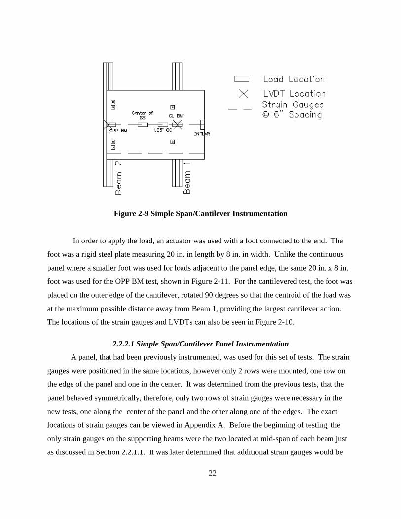
Figure 2-9 Simple Span/Cantilever Instrumentation

In order to apply the load, an actuator was used with a foot connected to the end. The

foot was a rigid steel plate measuring 20 in. in length by 8 in. in width. Unlike the continuous

panel where a smaller foot was used for loads adjacent to the panel edge, the same 20 in. x 8 in.

foot was used for the OPP BM test, shown in Figure 2-11. For the cantilevered test, the foot was

placed on the outer edge of the cantilever, rotated 90 degrees so that the centroid of the load was

at the maximum possible distance away from Beam 1, providing the largest cantilever action.

The locations of the strain gauges and LVDTs can also be seen in Figure 2-10.

2.2.2.1 Simple Span/Cantilever Panel Instrumentation

A panel, that had been previously instrumented, was used for this set of tests. The strain

gauges were positioned in the same locations, however only 2 rows were mounted, one row on

the edge of the panel and one in the center. It was determined from the previous tests, that the

panel behaved symmetrically, therefore, only two rows of strain gauges were necessary in the

new tests, one along the center of the panel and the other along one of the edges. The exact

locations of strain gauges can be viewed in Appendix A. Before the beginning of testing, the

only strain gauges on the supporting beams were the two located at mid-span of each beam just

as discussed in Section 2.2.1.1. It was later determined that additional strain gauges would be

23

added to Beam 1 in order to obtain more data about the beam behavior. These strain gauges

were placed in pairs every 1.5 ft along Beam 1. The exact locations of these gauges are detailed

in Figure A-6 in Appendix A. This addition was done to determine the moment along the beam

which will be discussed further in Chapter 3. All strain gauges used were manufactured by

Vishay Precision Group. LVDTs were also connected at the center span of each steel beam. The

same LVDT-connection was used as in the continuous panel configuration. The data acquisition

used was a Optim-Megadac 200. All strain gauges, the LVDTs, along with the load cell were

plugged into this system through channels.

2.3 Testing Procedure

2.3.1 Simple Span/Cantilever

The testing procedure began with the set up and positioning of the actuator. The actuator

was hung on a steel I-beam from which it could be slid transversely along the panel (North to

South). Once the actuator was slid into the desired loading location, the load cell and foot were

attached to it. Since the foot was rigid steel, a dense rubber mat was placed in-between the foot

and the panel to prevent damage that the foot might cause to the panel. The dense rubber mat

contained grooves which allowed for strain gauges and wires to be located underneath the foot.

Load was then gradually applied to the panel by the hydraulic actuator. The load would be

slowly increased to the desired level then held static for approximately 1.5 minutes. It was

necessary to wait this time at each load since the Optim Megadac 200 system took roughly 11

seconds to scan all the channels. Over a minute and a half, it would be possible to collect

roughly 9 data points. Load was then completely removed from the panel and the same

procedure was completed again to provide another set of data points to ensure the precision of

the data. It was noticed early on in testing that the panel behaved differently under various load

magnitudes. After this realization, it was decided to hold loads static at increments of 5 kips up

to a total of 20 kips. These four load levels represented the data points used for analysis.

2.3.2 Continuous Panel

The continuous panel test procedure was relatively the same as the Simple

Span/Cantilever, to the extent that the foot/actuator assembly would be placed then load would

be increased in increments and held static for a few minutes. When analyzing the data from

24

2007, it was apparent that the loads were increased and held static in smaller increments. For

example, the load would be increased to 2.5 kips and held static for a minute or two, then

increased another 2.5 kips. In order to analyze this data and compare to the data observed from

the simple span/cantilever tests, data points at 5, 10, 15 and 20 kips were the only data analyzed.

For the continuous panel, the load was increased to levels above 20 kips in some cases. Most

tests reach 25 kips and some went up to 30, however such data was not used in the analysis for

this thesis.

2.4 Data Analysis

After the data was collected from the computer connected to the Optim Megadac 200, it

was converted to a Microsoft Excel file to be analyzed. All strain gauge along with LVDT

readings were zeroed out using the first data point reading when no load was on the panel. This

took care of subtracting the panel dead weight when finding the beam reactions from the load

induced by the actuator. A dummy gauge was also placed on an additional H10 x 42 steel beam

that was not loaded. This strain, although its changes were small during testing, was subtracted

from every other strain value analyzed in order to account for temperature changes during that

particular test period. When analyzing a strain data points for a specific location at a particular

load, the values were checked against each other for precision then, once any floating values

were disregarded, the data was averaged for a final strain value.

25

CHAPTER 3 - Load Distribution on Steel Beams

When analyzing the continuous panel test data, the question was raised of how to

effectively analyze the data collected from testing. It was unknown how to calculate the load

each beam was resisting when given a strain value from the center span of a steel beam

supporting the panel. Consequently, it was decided to analyze the behavior each beam when

subject to different loads at various locations. In order to do this, using the simple

span/cantilever test set-up, moment curves were produced for an instrumented beam, Beam 1,

when subject to various loading conditions. This chapter presents the procedure used to

determine these moment curves along with a discussion of the results and conclusion from these

tests.

3.1 Determining Moments

The beam-moment analysis was done using the simple span/cantilever test configuration.

As discussed in Chapter 2, two strain gauges were mounted every 1.5 ft along Beam 1 for the

entire 12 ft span, as shown in Figure A-6 in Appendix A. Since two strain readings were taken

at every location, errors could be identified when the 2 strains were dissimilar. Theoretically, the

strain in the beam should be symmetrical about mid-span of the beam which allows for even

further comparison of the strain readings. With four strains at each location, faulty gauge

readings were identified and disregarded, which left the remaining readings to be averaged for a

final strain value for that particular location on the beam. For the most part, the strains were

within 10μЄ to 20μЄ of each other. Using these strain values, a moment was determined using

the following equations:

26

σ = EЄ =

[Equation 3-1(a)]

Solving for M:

M =

[Equation 3-1(b)]

Where σ = stress, E is equal to the modulus of elasticity, Є is equal to the strain, M is equal to the

moment, c is equal to the distance from neutral axis, and I is equal to the moment of inertia.

The values for “I” and “c” were 254.84.56 in.4 and 5.56 in. respectively as discussed in

Section 2.1.2. A moment curve was then produced through plotting these moments, which were

determined at 1.5 ft increments along Beam 1 resulting in 5 locations from beam end through

midspan. For all 5 loading locations, moment curves were produced for 4 different loading

magnitudes. For example, the moments were produced for the load of 5 kips in the loading

location of CL BM1 and a curve was produced. Next a moment curve was produced for a load of

10 kips at the loading location of CL BM1. This procedure was repeated for the other 3

locations along the simple span of the panel. After brief analysis of the moment curves for 5

kips, it was observed that the panel did not have a uniform behavior which produced erratic

curves. It was then decided to ignore such curves. This coincides with the unpredictable panel

behavior at low loads as discussed earlier in the Section 2.3.1. A moment curve was also

produced for the cantilever test at a magnitude of 15 kips.

3.2 Analyzing Moments

Three line graphs were used for the moment analysis at three different load levels (10, 15,

and 20 kips). For example, Figure 3-1 shows the moment graph for a 15 kip load, placed in

various positions along the panel centerline.

27

Figure 3-1 Beam 1 Moment Curve at Load Magnitude of 15 kips

After producing the moment curves using strain gauge readings, the next step was to

derive a loading scenario that would produce such shapes of these moments. Using Table 3-23

of the AISC Manual (Figure 3-2), the graph representing a uniform load partially distributed over

a beam would correspond to the experimental results.(AISC, 2008) For a uniform partially

distributed load on a beam, the moment curve is linear up to the point where the load begins,

then is parabolic just like any moment curve for a uniform load would be. Looking back to

Figure 3-1, for the most part, all 5 moment curves are somewhat linear for a period of length,

depending on the load location, and then appear to have a parabolic-type shape in the middle.

After this realization, straight lines were drawn on the curves to determine a point where the load

from the panel effectively started acting on the beams. This procedure is shown in Figure 3-3

below.

0

10

20

30

40

50

0 1 2 3 4 5 6 7 8 9 10 11 12

Mo

me

nt

(kip

*ft)

Position Along Beam (ft)

Moment Curves - 15 kips

CNTLVR

CL BM 1

1.25' OC

Center of SS

OPP BM

28

Figure 3-2 Shear, Moment, Deflection Diagram for Uniform Load Partially Distributed

(AISC, 2008)

Figure 3-3 Beam 1 Analyzed Moment Curves at Load Magnitude of 15 kips

(Additional Figures B-2 and B-3 contain moments curves at different load magnitudes)

05

101520253035404550

0 1 2 3 4 5 6 7 8 9 10 11 12

Mo

me

nt

(kip

*ft)

Position Along Beam (ft)

Moment Curves - 15 kips

CNTLVR

CL BM 1

1.25' OC

Center of SS

OPP BM

29

From Figure 3-3, panel load distribution lengths (i.e. the lengths of the assumed

uniformly distributed load) were selected. The point where the line appears to deviate from the

straight line was identified as the point at which the load started to act on the beam. For

example, for CL BM1, the moment curve seems to differ from the straight line drawn at roughly

4 ft into the curve. Since the curve is symmetrical, the curve would differ from a straight line

drawn on the other side at 4 ft into the curve as well. Since there are two linear sections of 4 ft, it

can be concluded that the panel is not acting on the beam for 8 ft of the beam’s 12 ft length.

Therefore, the remaining length of 4 ft, in the center section of the beam, is receiving the

distributive load from the panel.

Table 3-1 Panel Distribution Length on Steel Beams

10 kips 15 kips 20 kips Load

Location (ft) Length (ft) Load

Location (ft) Length (ft) Load

Location (ft) Length (ft)

0 4 0 4 0 3

1.25 4.4 1.25 4 1.25 3

3 6 3 6 3 6

6 6 6 6 6 6

As seen in Table 3-1, the distribution length for a 15 kip load 0 ft away from the beam is

4 ft as explained in the previous paragraph. The distance is “0 ft” because the loading position is

CL BM1 which is directly over the instrumented beam, Beam 1. Likewise, a load location of

1.25 ft in Table 3-1 corresponds to loading location 1.25’ OC BM1 and a load location of 3 ft

corresponds to the loading location Center of SS. The same procedure was followed in finding

all of the distribution lengths that are shown in Table 3-1. The moment curves for other load

magnitudes are located in Appendix B-1. It can be argued that each moment curve contains a

certain degree of curvature even in the locations that were stated as being linear in Figure 3-3. In

reality, this is true, as the panel is not acting on the beam as a perfect uniform load starting at a

specified location and ending at another. There is likely some change in the magnitude of the

distributive load that starts small at the edge of the panel with a peak magnitude at the center.

Since it would be quite difficult to compute a load from such an irregular loading pattern, the

procedure of finding a uniform partially distributive load is much more manageable. Similar

engineering procedures are used commonly such as assuming the effective compressive force in

30

a flexural concrete member to be 85% of the actual compression depth, using the Whitney Stress

Block. With these distribution lengths determined, it was possible to calculate the load each

beam was resisting in the corresponding testing scenario.

3.3 Determining Beam Loads

Using the distribution length from the moment curves determined for Beam 1, the actual

load that each beam was resisting in a given test could be calculated. Since there weren’t strain

gauges at 1.5 ft increments on the other beams for each test, the moments had to be determined

based on the strain gauges available at the mid-span of the beam. (These are Beam 2 for the

simple/cantilevered test configuration, and Beam 2 through Beam 4 for the continuous panel test

configuration.) Using these strains, the stress at that location could be calculated just by

multiplying by the modulus of elasticity, 29,000 ksi. With the knowledge that the stress is also

related to the moment, a moment could be calculated as shown in Equation 3-1. After this

moment is computed, determining the magnitude of the uniform load, w, is relatively simple as

shown in Figure 3-4. Equation 3-2 shows the final equation used to determine the load resisted

by beams in all the tests. When considering a particular test, besides the varying strain from

different load circumstances, the “ℓ” factor would be the only variable that changed from beam

to beam. The value of “ℓ” is taken from Table 3-1. The total load on the beam is wℓ.

Figure 3-4 Moment Calculation

31

wℓ =

[Equation 3-2]

Using Equation 3-2 to substitute for “M,” the load resisted by the steel beam becomes:

wℓ =

[Equation 3-3]

32

CHAPTER 4 - Simple Span/Cantilever Testing

This chapter will analyze the results from the tests conducted in the fall/winter of 2010

into early January, 2011. The test set ups, as discussed in Chapter 1 consisted of a simple span

panel with a 2.33 ft cantilever on one side. Although this data was collected roughly 3 years after

the previous tests were done in 2007, it is important to analyze it first in order to establish a

conservative-base distribution factor that can be compared with the continuous panel analysis.

Load resisted by the two steel beams was determined for 4 different loading scenarios shown in

Figure 2-11. (CL BM 1, 1.25’ OC, Center of SS, and OPP BM) After this, the panel was

modeled somewhat as a continuous panel. Using this model, wheel loads were modeled and a

load distribution ratio was determined from the analysis. The analysis of the cantilever load

scenario served as a validation to support the data. The procedures used to complete these steps

are discussed in the following sections.

4.1 Distribution Lengths and Determining Loads

The second part of Equation 3-2 was used to calculate the load resisted by each beam.

This procedure is illustrated as follows. For example, when a load of 15 kips was directly over

Beam 1, or loading “CL BM 1,” the average strains at the center span of Beam 1 and Beam 2

were 291 μЄ and 22 μЄ respectively (Data CD). Using Table 3-1, the distribution lengths for

Beam 1 and Beam 2 with a 15 kip load were 4 ft and 6 ft respectively. The 4 ft distribution

length was used because the load was acting 0 ft away from (i.e. directly on top of) Beam 1, and

the 6 ft was used given that the load was acting 6 ft away from Beam 2. Substituting these

values into Equation 3-3, a load that each beam was resisting is found. This same procedure was

used to calculate the beam loads for the rest of the loading cases in this test set-up. The

cantilever wasn’t used for this particular analysis, however, the results will be discussed in

Section 4.4.

The results from this procedure are given in Table 4-1 below. Initial assessment of the

results reveals inaccuracies between the stated loads for each test and the total load that was

applied on the panel. For instance, when the 15 kip load was applied over Beam 1, the sum of the

loads on the two support beams is equal to 13.4 kips. This difference is attributed to

experimental error as well as panel behavior. The procedure for finding the beam reactions uses

33

the distribution lengths found in Chapter 3. As discussed previously in Chapter 3, using a

uniform load with a particular length is an approximate method to find the beam reactions and

does contain some experimental and modeling errors.

34

4.2 Simple Span Load Distribution

The load resisted by each beam, or termed “beam reactions”, were determined for all four

simple span load scenarios that were tested (CL BM1, 1.25’ OC BM1, Center of SS, and OPP

BM), which were then used to produce a load distribution factor that could be compared with

other bridge deck materials in the AASHTO code. In order to produce these ratios, line graphs

were made for each load level analyzed (10, 15, and 20 kips) comparing the load ratios. These

are shown in the center section of Table 4-1, and the distance from Beam 1where the load was

applied. Beam 1 was modeled as the “design beam.” This means that the load ratio charts (as

will be shown later in Figure 4-1) are based on how far the load is acting from Beam 1 (x-axis

value). The graphs model how much load would be transferred to Beam 1 when a single load is

placed on the panel at a certain location. For example, when a 15 kip load is placed 5.33 ft away

from Beam 1, then the load ratio would be 0.15. Another way to look at this is that 15% of that

15 kip load placed on the panel 5.33ft away was resisted by Beam 1. Likewise, if a 15 kip load

was placed 1.25 ft away on the panel, then the resulting load ratio would be 0.82. The x-values

of the four data points on the graph consist of 0 ft, 1.25 ft, 3 ft, and 5.33 ft which are the

locations away from the design beam where the load is applied. (Note that the load distance

corresponding to the OPP BM loading position was 5.33 ft away from the design beam rather

than being the entire 6 ft span since the centroid of the loading foot was not directly over the

center line of Beam 2 as shown in Figure 2-9.) In order to estimate the load ratio associated with

any distance between these four data points, a 2nd

-degree polynomial was generated as a best fit

curve through these points. It is important to note that these equations are only valid for

distances from 0 ft to 6 ft. Theoretically, the ratio in the center of the simple span should be

0.500 (each beam takes half the load) however the highest collected ratio was taken. This was

done to keep a consistent procedure for analyzing data. It was also observed that if the data point

was reduced to 0.55, it would produce a less conservative line of best fit curve.

35

(a)

(b)

(c)

Figure 4-1 Load Ratio Graphs for a Load Magnitude of (a) 10 kips, (b) 15 kips, and

(c) 20 kips - Simple Span Analysis

0.90.83

0.58

0.17

y = -0.0148x2 - 0.0604x + 0.90880

0.2

0.4

0.6

0.8

1

0 1 2 3 4 5 6R

atio

Location of Load Along Panel (ft)

0.920.82

0.56

0.15

y = -0.0119x2 - 0.0829x + 0.92680

0.2

0.4

0.6

0.8

1

0 1 2 3 4 5 6

Rat

io

Location of Load Along Panel (ft)

0.930.82

0.55

0.14

y = -0.0107x2 - 0.0931x + 0.93710

0.2

0.4

0.6

0.8

1

0 1 2 3 4 5 6

Rat

io

Location of Load Along Panel (ft)

36

In order to get a load distribution ratio from the data shown in Figure 4-1, different

loading scenarios would have to be analyzed and the most critical case would be selected. The

critical case refers to the maximum ratio of the amount of load the design beam is taking to the

amount of loading being applied on the panel. As discussed earlier in this thesis, the standard

AASHTO truck has a wheel spacing of 6 ft and truck spacing of 4 ft. Therefore to get the most

realistic value, two loads would have to be analyzed per scenario. Since the plotted ratios on the

line graphs in Figure 4-1 are not all in perfect 6 ft increments, the equations for the polynomial

lines of best fit will be used. For example, to analyze the scenario where one wheel (20 kips)

was placed at CL BM1, or 0 ft away from the design beam, then the ratio would be equal to the

sums of plugging 0 and 6 into the equation shown in Figure 4-1(c), y=-0.0107x2 – 0.0931x +

0.9371. The “6 ft” value was used in the equation to model the other truck’s wheel at a distance

of 6 ft away. The schematic for the standard AASHTO truck is shown in Figure A-20 in

Appendix A-3. In order to analyze a case where a 20 kip wheel load was 1 ft away from the

design beam, the values of “1” and “5” were used in the equation shown in Figure 4-2. The

values of 1 and 5 were used to simulate the wheel load 1 ft away on one side of the beam and

another wheel load 5 ft away on the opposite side of the beam making a total distance of 6 ft

between the wheel loads. Although it is conservative to model the data from the simple span as a

continuous span, it was necessary to use a conservative value initially that could be later

compared to the continuous test data. Just as the values of “1” and “5” were added together for a

loading scenario, so were the values of “2” and “4” as well as “3” and “3.” The results of these

calculations are shown in Table 4-2.

The AASHTO code has different design factors for two different types of bridges, one for

bridges with single lanes of traffic and the other for bridges with multiple lanes of traffic. For

the case of a bridge bearing multiple lanes of traffic, it was necessary to apply extra wheel loads

to the distribution factor. These wheel loads would theoretically be placed at distances of 4 ft

from the outside wheel load to model another truck. Due to the size of the panel and the testing

facilities, the results of this thesis are applicable for design factors considering one traffic lane

only.

37

Table 4-1 Simple Span Load Distribution

Design Case for Interior Beam Spacing = 6'

10 kips 20 kips Equation for Magnitude of Load with Relevance to Distance from

Design Beam: Magnitude = -0.0148x2 - 0..0604x+0.9088

Equation for Magnitude of Load with Relevance to Distance from Design Beam: Magnitude = -0..0107x2 -

0..0931x+0..9371

Wheel Load Locations (ft)

Load Magnitude

Wheel Load Locations (ft) Load Magnitude

0 0.92 0 0.93

1 1.07 1 1.04

2 1.16 2 1.10

3 1.19 3 1.12

Critical Design: 1.19 Critical Design: 1.12

Design Equation: S/ 5.05 Design Equation: S/ 5.34

15 kips Critical Design Value for Interior Beam

(6' Spacing) Equation for Magnitude of Load with Relevance to Distance from

Design Beam: Magnitude = -0.0119x2 - 0..0829x+0.9268

S/ 5.05

Wheel Load Locations (ft)

Load Magnitude

0 0.93

1 1.05

2 1.12

3 1.14

Critical Design: 1.14

Design Equation: S/ 5.25

From Table 4-2, the most critical load distribution ratio was found to be S/5.05 or S/5.

This was formulated from the scenario where two 10 kip loads were modeled to be 3 ft on either

side of the beam producing a ratio of 1.19. This means that the design beam, which had the two

10 kip loads on either side, would be designed for 1.19*10 kips for a total of 11.9 kips. The “S”

ratio may be derived from the load ratio of 1.19 since the beam spacing is 6 ft, S/5.05 is found by

setting 6/x = 1.19 and solving for x.

4.3 Cantilever Analysis

It was originally thought that the cantilever analysis would provide data for a design ratio

to be used when considering an exterior beam. Upon further research and discussion with

practicing engineers, it was found that simple statics calculations are used to determine the

38

design load for an exterior beam with a cantilever. Since the data collected from the cantilever

would not be used to produce a load distribution ratio, it was used primarily to validate test

results. The reactions of the two beams were based on the measured strains at mid-span of each

beam - when a load was placed on the cantilever. These reactions were then compared to values

derived from static calculations. The beam reactions along with ratios are shown in Table 4-3.

Since the sum of the beam reactions does not add up to the total load put on the beam, these

normalized load ratios provide an estimate of the portion of the load one beam is taking

compared to the other beam. The beam distribution length used for Beam 1, on the cantilever

side, is based on the moment curve labeled “CNTLVR” for the 15 kip graph in Figure 3-3. The

procedure followed is the same as the one that was used to produce the graphs of Figure 4-1.

Table 4-2 Cantilever Ratios

Reactions (kips) Ratios of Load Taken By Each Member

Load Beam 1 Beam 2 Sum Load Beam 1 Beam 2 Sum

0.0 0.00 0.00 0.00 0.0 0.00 0.00 0.00

1.1 0.83 -0.40 0.43 1.1 1.94 -0.94 1.00

2.1 1.45 -0.54 0.91 2.1 1.59 -0.59 1.00

3.1 2.48 -0.67 1.81 3.1 1.37 -0.37 1.00

4.1 3.43 -0.94 2.49 4.1 1.38 -0.38 1.00

5.3 4.55 -1.34 3.21 5.3 1.42 -0.42 1.00

6.2 5.47 -1.81 3.66 6.2 1.49 -0.49 1.00

7.2 6.47 -2.34 4.13 7.2 1.57 -0.57 1.00

8.3 7.62 -2.75 4.88 8.3 1.56 -0.56 1.00

9.3 8.81 -3.08 5.72 9.3 1.54 -0.54 1.00

10.3 9.99 -3.75 6.24 10.3 1.60 -0.60 1.00

11.4 11.17 -3.82 7.35 11.4 1.52 -0.52 1.00

12.4 12.26 -4.35 7.91 12.4 1.55 -0.55 1.00

13.4 13.50 -4.89 8.61 13.4 1.57 -0.57 1.00

14.4 14.69 -5.22 9.46 14.4 1.55 -0.55 1.00

Max: 1.60 -0.60

Min: 1.37 -0.37

From Table 4-3, the Load Ratios are listed for a load ranging from 1 to 14.5 kips. From a

simple static calculation, the load ratio for Beam 1 should be 1.33P while the load ratio for Beam

2 should be -0.33P. From the Table, it can be concluded that these ratios are consistently within

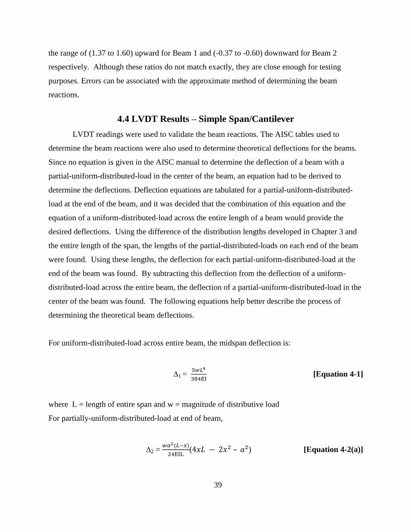
39

the range of (1.37 to 1.60) upward for Beam 1 and (-0.37 to -0.60) downward for Beam 2

respectively. Although these ratios do not match exactly, they are close enough for testing

purposes. Errors can be associated with the approximate method of determining the beam

reactions.

4.4 LVDT Results – Simple Span/Cantilever

LVDT readings were used to validate the beam reactions. The AISC tables used to

determine the beam reactions were also used to determine theoretical deflections for the beams.

Since no equation is given in the AISC manual to determine the deflection of a beam with a

partial-uniform-distributed-load in the center of the beam, an equation had to be derived to

determine the deflections. Deflection equations are tabulated for a partial-uniform-distributed-

load at the end of the beam, and it was decided that the combination of this equation and the

equation of a uniform-distributed-load across the entire length of a beam would provide the

desired deflections. Using the difference of the distribution lengths developed in Chapter 3 and

the entire length of the span, the lengths of the partial-distributed-loads on each end of the beam

were found. Using these lengths, the deflection for each partial-uniform-distributed-load at the

end of the beam was found. By subtracting this deflection from the deflection of a uniform-

distributed-load across the entire beam, the deflection of a partial-uniform-distributed-load in the

center of the beam was found. The following equations help better describe the process of

determining the theoretical beam deflections.

For uniform-distributed-load across entire beam, the midspan deflection is:

∆1 =

[Equation 4-1]

where L = length of entire span and w = magnitude of distributive load

For partially-uniform-distributed-load at end of beam,

∆2 =

( – ) [Equation 4-2(a)]

40

where a = length of distributive load, x = location of desired deflection

Substituting “x=L/2” to find the deflection at mid-span,

∆2’ =

[Equation 4-2(b)]

By superposition, the total theoretical deflection at mid-span,

∆Theoretical = ∆1 - 2∆2’ [Equation 4-2]

The value of “L” is to be taken as 12 ft and the “a” value in Equation 4-2 is equal to: 12 ft

– the distributive length (determined in Chapter 3) since there is a load on each side of the beam.

The value for “w” is the same in both Equation 4-1 and Equation 4-2, for the purpose of

subtracting out the deflection due to load on the sides of the beam. “E” was taken as 29,000 ksi

and “I” was taken as 254.84 in.4 These theoretical deflections were then graphed against the

experimental deflections to evaluate the adequacy of the method of determining beam reactions

developed in Chapter 3. Figure 4-2 and Table 4-4

Table 4-3 show the results of the 1.25’ OC loading scenario. As it can be seen, the

experimental and theoretical deflections for CL BM1 were very similar. The Beam 1 deflections

do start to stray away from each other after a load of 10 kips is reached. This may be due to the

change in load distribution lengths. Even though the percent error is around 30% for the higher

loads, the difference in deflection at a load magnitude of 20 kips, is only 0.079 in. The

deflection graphs and tables for the rest of the loading scenarios can be found in Appendix C. For

the most part, when reviewing the deflection results from the other loading scenarios, the percent

error does not go above 30% and usually stays under 20%. When it does exceed 30%, it is high,

around 80%, which is due to the miniscule amount of deflection, such as 0.002 in.Even such

relatively small values may produce high % error readings. With this in mind, the high percent

errors in these circumstances is acceptable.

41

Figure 4-2 Experimental vs. Theoretical Deflections – CL BM1 – Simple Span

Table 4-3 Experimental vs. Theoretical Deflections – CL BM1 – Simple Span

Deflections - Theoretical vs. Experimental

Load

Theoretical Experimental % Error

Beam 1 Beam 2 Beam 1 Beam 2 Beam 1 Beam 2

5.3 0.055 0.006 0.052 0.002 5.38% 74.36%

10.3 0.110 0.010 0.093 0.002 15.38% 83.52%

15.6 0.183 0.011 0.135 0.002 25.93% 84.89%

20.8 0.257 0.014 0.178 0.002 30.81% 88.46%

-0.050

0.000

0.050

0.100

0.150

0.200

0.250

0.300

5.0 10.0 15.0 20.0D

efle

ctio

n (

inch

es)

Load (kips)

Beam 1 Theo

Beam 1 Exp

Beam 2 Theo

Beam 2 Exp

42

CHAPTER 5 - Continuous Panel Testing

This chapter will outline the procedure used for data analysis, as well as the

corresponding results of the 2007 continuous panel tests.

Load resisted by the four steel beams was determined for 5 different loading scenarios.

(CL BM1, MS 1-2, CL BM2, MS 2-3, and CL BM3) Just as was done in Chapter 4, the panel

load ratios were determined, then different loading scenarios were produced. From these loading

scenarios, load distribution factors were found. The process of determining these factors will be

discussed in this chapter.

5.1 Load Distribution on Beams

Beam reactions were determined for the data collected from the continuous panel testing

using the same distribution lengths that were determined in Chapter 3. Even though these

distribution lengths were obtained through testing on a simple span rather than a continuous

panel, it was decided that they would be adequate for this analysis. Just as in the simple span

analysis, the strain reading used to determine the beam reactions was collected at the mid-span of

the beam. The same equations were also used to determine the beam reactions in the continuous

analysis as were used in the simple span analysis.

5.2 Continuous Panel Analysis

A similar method was used to determine the load distribution ratios for the continuous

panel as the method used for the simple span. The main difference between the continuous

analysis and the simple span analysis is that the polynomial line of best fit equations were not

used to determine the load ratios. Since loads were placed at the mid-spans of every span along

with on top of every beam along the panel, it proved to provide enough data points to combine

for load ratios. For this reason, interpolation using the best fit curves was not necessary. The

analyzed loading scenarios used only loads at distances that had been tested and had resulting

corresponding data. Figure 5- analyzes different loading scenarios for Beam 1.

43

Figure 5-1 Loading Scenarios - Beam 1 – Load Magnitude: 20 kips

(a)

(b)

Figure 5-2 Load Ratio for (a)Beam 1 and (b)Beam 4 for Load Magnitude of 20 kips

0, 0.676

1.25, 0.479

2.5, 0.297

4.25, 0.146

6, 0.000

y = 0.0095x2 - 0.1682x + 0.6731

0.0

0.1

0.2

0.3

0.4

0.5

0.6

0.7

0.8

0 1 2 3 4 5 6

Rat

io

Location of Load Along Panel

-8.5, 0.009-7.25, -0.031 -6, -0.004

-4.25, 0.096

-2.5, 0.321

y = 0.017x2 + 0.2392x + 0.8107

-0.1

0.0

0.1

0.1

0.2

0.2

0.3

0.3

0.4

-9 -7 -5 -3

Rat

io

Location of Load Along Panel

44

The first line graph in Figure 5- represents the load ratios obtained for Beam 1 when the

load is placed along the panel at various locations. This curve compares the load resisted by

Beam 1 to the total load placed on the panel. For example, for the first graph which is plotted for

Beam 1, when the load is placed 0 ft away, the y-coordinate of line graph is at 0.676 which

means Beam 1 is taking 67.6% of the load at this location. Shown above in Figure 5-1, the

different loading scenarios are analyzed for Beam 1. These scenarios include modeled wheel

loads that are 0 ft, 1.25 ft, 2.5 ft and 4.25 ft away from the design beam, or in this case, Beam 1.

The second line graph in Figure 5-2 represents load ratios for Beam 4 corresponding to

various loading locations along the panel. This line graph is the same as the first line graph

except for the range of the x-axis values. Since Beam 4 is located 8.5 ft from Beam 1 (Beam 1 is

treated as the starting point of the x-axis), all the x values are negative. For example, the

coordinate point on the graph representing the load ratio when a load is placed over Beam 3 is (-

2.5, 0..321) since Beam 3 is located 2.5 ft from Beam 4 and the load ratio is 0.321. This means

that Beam 4 is taking 32.1% of the total load when a load is placed over Beam 3. Likewise, a

coordinate point on this graph with an x-value of “-8.5” would correspond to a load ratio for

Beam 4 when the load is directly over Beam 1. This same coordinate system is applied for line

graphs representing load ratios for Beam 2 and Beam 3 in Appendix C.

In order to model a truck on the panel, a wheel load is 0 ft away, or directly over Beam 1,

and a load 6 ft away are added together (modeling the 6 ft truck wheel spacing). Since there

were no load scenarios for load in the mid-span of Beams 3 and 4 or directly over Beam 4, the

beam reactions from Beam 4 were used for these ratios. For example, when considering the

design of Beam 1, it would be necessary to analyze the effects of the combination of a load 2.5

ftaway along with 8.5 ft (modeling the truck axle with 6 ft spacing). In this case, the load ratios

from Beam 4 would have to be taken into account. Since there were not tests with load 8.5 ft

away from Beam 1, the reaction of Beam 4 when a load was directly over Beam 1 would be

taken into account. This is easier to visualize when looking at Figure 5-1. The ratio for Beam 1

when the load is directly over Beam 4 is 0.009. Referencing this value of 0.009 back to the chart

in Figure 5-2 titled “20 kips BM 4,” the load ratios including the effect of the second wheel of

the truck axle become:

45

0.306

Table 5-1 shows the Distribution Summary for Beam 1. This includes the load ratios for

all loading scenarios along with the corresponding S ratio. The average critical design value

was S/4.6 for Beam 1.

Table 5-1 Load Distribution Summary for Beam 1

Simulated Wheel Load 10 kips 15 kips 20 kips

Location of First Wheel Along Panel (ft)

Load Ratio

S Ratio

Load Ratio

S Ratio

Load Ratio

S Ratio

0 0.63 S/4.7 0.66 S/4.5 0.68 S/4.4

1.25 0.48 S/6.3 0.48 S/6.2 0.48 S/6.3

2.5 0.33 S/9.1 0.31 S/9.6 0.31 S/9.8

4.25 0.19 S/16.1 0.16 S/18.6 0.15 S/20.5

Critical Design Value: 0.63 S/4.7 0.66 S/4.5 0.68 S/4.4

Controlling Critical Design Value: S/4.4 Average Critical Design Value: S/4.6

It is possible to see unequal values for beam spacing on some bridges. This is not

uncommon in some older bridges. After inquiring with local engineers, the researchers at KSU

determined using the average of the beam spacing’s would be adequate for this analysis.

Therefore, when computing the S ratio, the spacing value used was 3 ft (average of 2.5 ft and 3.5

ft). The same procedure was used for the analysis of Beam 2 which can be seen in Figure 5-3

through Figure 5-5 seen below. The line graphs in Figure 5-2 start at -2.5 ft on the horizontal

axis and go up to 3.5 ft. Referring to Figure 2-9, the axis starts negative because anything on the

Beam 1 side of Beam 2 is considered to be negative, therefore the point at -2.5 ft is when the

load is located over Beam 1. Just as data from the load ratios for Beam 4 was used in the analysis

of Beam 1, data from Beam 3 must be used for the analysis of Beam 2. When modeling a wheel

load directly over Beam 2, the load ratio for a load directly over Beam 2 must be added to a load

ratio for a load 6 ft away (modeling the other wheel on the axle). Since there was no load placed

6 ft away from Beam 2, a load ratio for Beam 3 from a load placed over Beam 1 was used. For

Figure 5-1 and Figure 5-3, the ratio for the load directly in the center of the panel (4.25 ft for

Figure 5-1 and 1.75 ft for Figure 5-3) contains only one load ratio. There was no data that could

be modeled as a load 6 ft away and subsequently it was decided that load would stand alone.

46

Figure 5-3 Loading Scenarios – Load Magnitude: 20 kips

(a)

(b)

Figure 5-4 Load Ratios for (a) Beam 2 and (b) Beam 3 for Load Magnitude of 20 kips

-6, 0.027 -4.75, 0.074

-3.5, 0.175

-1.75, 0.354

0, 0.506y = 0.0049x2 + 0.1126x + 0.5148

0.0

0.1

0.2

0.3

0.4

0.5

0.6

-6 -5 -4 -3 -2 -1 0

Rat

io

Location of Load Along Panel

47

Table 5-2 Load Distribution Summary for Beam 2

Simulated Wheel Load 10 kips 15 kips 20 kips

Location of First Wheel Along Panel (ft)

Load Ratio

S Ratio

Load Ratio

S Ratio

Load Ratio

S Ratio

-2.5 0.49 S/6.2 0.47 S/6.4 0.46 S/6.5

-1.25 0.55 S/5.5 0.55 S/5.5 0.55 S/5.4

0 0.45 S/6.6 0.56 S/5.4 0.56 S/5.4

1.75 0.35 S/8.6 0.38 S/7.8 0.40 S/7.4

Critical Design Value: 0.55 S/5.5 0.56 S/5.4 0.56 S/5.4

Controlling Critical Design Value: S/5.4 Average Critical Design Value: S/5.4

5.3 LVDT Results – Continuous Panel

The same approach and equations were used to determine the deflections for the

continuous panel tests as were used for the simple span and detailed in Section 4.4. Just as was

done in the simple span analysis, the theoretical deflections were graphed and tabulated against

the experimental deflections. An example of this can be seen in Figure 5-3 and Table 5-3 for the

loading scenario, CL BM1. The theoretical and experimental deflections are not as close as they

were for the simple span, reaching 45% error (0.154 in.) in some circumstances as seen below

for Beam 1 at a load of 20 kips. The deflection tables and charts for other loading scenarios are

located in Appendix C. The percentage of errors generally stayed under 40% and dropped as

low as 20% and less for the MS 2-3 loading scenario. For the deflections of beams that had load

directly over them, the % error ranged from 35-40%. For the beams adjacent to the beams with

load directly over them, the percent error was usually around 20%. However, if the adjacent

beam was greater than 3 ft away, the percent error increased to around 40%. The maximum

percent error where the deflection values are small, in such cases as Beam 3 and Beam 4 below,

can be ignored. Error can also be attributed to the beam reactions not being exact as well as

some error in the LVDT’s reading the deflection.

48

Figure 5-5 Deflections - CL BM1 - Cont. Test

Table 5-3 Experimental vs. Theoretical Deflections - CL BM1 - Cont. Test

Deflections - Theoretical vs. Experimental

Theoretical Experimental

Load Beam 1 Beam 2 Load Beam 1 Beam 2

5.0 0.071 0.035 5.0 0.044 0.028

10.1 0.154 0.062 10.1 0.093 0.051

15.1 0.244 0.090 15.1 0.143 0.072

20.0 0.346 0.120 20.0 0.192 0.092

Load Beam 3 Beam 4 Load Beam 3 Beam 4

5.0 0.006 0.004 5.0 0.000 -0.005

10.1 0.008 0.004 10.1 0.000 -0.009

15.1 0.010 0.003 15.1 0.000 -0.012

20.0 0.010 0.003 20.0 -0.002 -0.017

% Error Load Beam 1 Beam 2 5.0 37.19% 20.31% 10.1 39.71% 17.61% 15.1 41.43% 20.37% 20.0 44.63% 23.48% Load Beam 3 Beam 4 5.0 100.00% 227.92% 10.1 100.00% 324.65% 15.1 104.66% 451.97% 20.0 115.99% 649.15%

-0.075

-0.025

0.025

0.075

0.125

0.175

0.225

0.275

0.325

0.375

5 10 15 20D

efle

ctio

ns

(in

)

Load (kips)

Beam 1 Theo

Beam 1 Exp

Beam 2 Theo

Beam 2 Exp

Beam 3 Theo

Beam 3 Exp

Beam 4 Theo

Beam 4 Exp

49

CHAPTER 6 - Panel Strain Analysis

Due to time constrictions and the fact that panel strains were not pertinent to the

objectives of this thesis, the panel strain was not analyzed in depth and needs further analysis.

The two panel strain graphs that are included in this thesis were generated from tests conducted

in 2007. In these two tests, the load was placed on the tongue edge of the panel. Besides the

location of the load, the test set up was the same as detailed in Appendix A for the continuous

panel test. Each graph title contains the load location. For example, a graph titled “Panel Strain

– Tongue Edge – Center of Beam 2,” signifies the load was placed along the center-line of Beam

2 longitudinally and was placed on the tongue edge of the panel transversely. Positive strains

recorded signify tension while negative strains signify compression. Both strain graphs are for

the top surface strain of the panel. Panel strain data exists for all the tests completed in 2007

and is available for each test on the (Data CD). The two representative graphs provide data for

the two different loading locations specified.

6.1 Tongue Edge – Center of Beam 2

Figure 6-1 Panel Strain for Load at Tongue Edge above BM 2 at a Load Magnitude of 22

kips

50

When the load was placed directly over Beam 2 on the tongue edge, there was a

significant amount of strain present in the panel, even though it was supported by a beam at that

location (Figure 6-1). The strain reached a maximum compression value of approximately 1000

μЄ at the point of loading. The strain decreased almost to zero traveling longitudinally along the

tongue edge towards Beam 1. The strain in the opposite direction, towards Beam 3, also

gradually reached zero at the Beam 3 support. From these observations, it is evident that the

panel had compressive strain on the top surface until it reaches an adjacent support, after which it

changed to tension. Consequently, the effective span length was confirmed to be the distance

between Beam supports since the strain reading had an inflection point at those locations. It is

important to note that the strain gauges were placed 6 in. on center in each longitudinal row,

therefore, it is likely that the inflection point was not directly at the beam support, but was within

6 in. on either side of the beam. The longitudinal strains seemed to somewhat converge to zero

traveling transversely across the panel toward the groove edge. Comparison of the strains

provided in this graph in both directions indicates that they appear to vary in a linear fashion,

however some outlying data points are present making it impossible to confirm this with the

strain gauges provided.

51

6.2 Tongue Edge – MS 2-3

Figure 6-2 Panel Strain for Load at Tongue Edge of MS 2-3 at a Load Magnitude of 22 kips

Panel strain data was collected for the second graph considering a load at mid-span along

the panel in between Beam 2 and Beam 3 (Figure 6-2). The maximum compressive strain

occurred at the point of loading with a magnitude of approximately 1700 μЄ. This higher strain

reading can be attributed to the lack of support under the load, therefore allowing a greater

deflection at that point. Similar to the previous graph, the strain, in general, varies linearly until

it reaches zero at the adjacent supports. On either side of the supports, tensile strain is present

from the negative moment induced due to the panel having a continuous support condition.

These results confirm that the effective span length is the distance between adjacent supports as

was found in the previous test. This is because the panel appears to be directly resisting the load

throughout the whole span since it is in compression in this area and switches to tension in the

adjacent span. The change occurs at the beam supports. The strain slowly converges to zero

transversely across the panel as well.

52

CHAPTER 7 - Conclusions

Two FRP panels were tested using two different support configurations. The continuous

panel test was completed throughout the year of 2007 while the simple span and cantilever tests

were completed November, 2010 through January, 2011. Load increments of 5 kips from 0 to 20

kips were analyzed in this thesis. From strain results, load ratios for beams were developed and

a distribution ratio for each tests setup was determined. Additional testing was completed on the

simple span in order to determine the moment curve for a beam with different loading scenarios.

These moment curves provided the researchers with insight that would determine an effective

load distribution length of the panel bearing on the supporting beam. The following sections

will discuss the conclusions drawn from the experimental research completed for this thesis.

The experiments conducted to determine the moment curves of the exterior beam

for the various loading scenario proved that the effective load distribution length

is shorter than the panel bearing length (<6 ft) when the position of the load is

near or on top of the beam, and that it increases until it reaches the entire length of

the panel (6 ft) at a loading distance of 3 ft or more away from the beam.

The load distribution lengths determined from the moment curves were used to

determine the beam reactions using the strain reading at the center line of the

beam. In order to validate these beam reactions, LVDTs were used to measure

deflection at mid-span of each beam supporting the FRP panel. These deflections

were compared against “theoretical deflections” which were determined from

substituting the beam reactions into beam deflection equations as described in

Section 4.4. For the simple span/cantilever analysis, the percentage of error for

the deflections was generally under 30%. At times when the two values differed,

the theoretical deflection frequently had a larger value than the experimental

deflection at loads of 10 kips and higher. This can be attributed to the load

distribution lengths values being too large for these loads and creating a higher

beam reaction which in turn would create a larger theoretical deflection.

53

The load distribution factor determined in the simple span analysis was “S/5”

where S is the longitudinal beam spacing. Although this ratio may be too

conservative, this value was established for the purpose of providing a benchmark

for comparing the results from the continuous panel. The AASHTO Specification

load distributions range from S/4 to S/6 for a timber deck, and S/6 to S/8 for a

concrete deck, depending on the support materials and conditions. Based on the

simple span analysis described in this chapter, the FRP deck performed more like

a timber deck rather than a concrete deck.

Although the cantilever tests validated the results to a certain degree, the reactions

do not entirely concur with expected results using a simple statics calculation.

While the load ratios for the beam on the side of the cantilever should have been

1.33, they averaged around 1.45 in the experiment. The ratios for the beam on the

opposite side of the cantilever, theoretically, should have been -0.33, however

they averaged around -0.45. Although these ratios are off by around 0.12, they do

show that the variations of the experimental beam reactions are consistent and in

the range where they should be.

The deflections of the continuous panel test were very similar to the simple span

deflections. The percent errors for the continuous test were, in general, 40% and

lower. The theoretical deflections were usually larger than the experimental

deflections, just as it was observed in the simple span analysis. In both cases, this

can be attributed to large load distribution lengths. The higher percent error is

due to the load distribution lengths being determined for a simple span test and

not for a continuous panel test. It is important to recognize that the theoretical

deflections are consistently above the experimental beams for all the beams in all

the loading scenarios. Consequently, the load ratios determined for the analysis

should be valid. Even though the beam reactions were somewhat large, they were

consistently larger than they should have been for all the beams analyzed based

on the deflection analysis.

54

For the continuous panel load distribution factor determination, the final

controlling values for the exterior and interior beams are S/4.6 and S/5.4

respectively. As expected, the panel behaved symmetrically; wheel load

distribution factors for opposite exterior beams and opposite interior beams

closely resembled each other. Unlike the results from the simple span testing, the

critical wheel load distribution occurred, for the most part, when the load was

directly over the design beam rather than when the load was in the center of the

spans. This is due to the close spacing of supporting beams and might not be the

case if the beams were spaced at larger intervals greater than the 6 ft wheel

spacing. These results confirm the previously stated values of S/5 when modeling

a simple span as continuous in Chapter 4.

The brief analysis of the panel strain shows that the spans, in between supports,

resisted the load for the entire length of the span. This conclusion was made since

when a load is applied in the middle of a span, the top panel surface has

compressive strain for the entire length of the span and tensile strain in the

adjacent span. This validates the method of using the entire span distance as the

effective beam spacing when determining the load distribution factors. Since the

strain gauges were spaced at 6 in. on center, the location of the strain inflection

points were only accurate to within 6 in. and the exact location remains unknown.

Further research should be done in this area using strain gauges placed at closer

intervals.

55

CHAPTER 8 - Bibliography

Alampalli, S., & Kunn, J. (2001). Load Testing of an FRP Bridge Deck Located on a Truss

Bridge. New York State Department of Transportation, Transportation Research and

Development Bureau, Albany, New York.

American Association of State Highway and Transportation Officials (AASHTO, 2010). (2010).

Standard Specifications for Highway Bridges (17th ed.). Washington D.C.

American Institute of Steel Construction Inc.: Steel Construction Manual (13th Edition ed.).

(2008).

Bakis, C. E., Bank, L. C., Brown, V. L., Cosenza, E., Davalos, J. F., & Lesko, J. J., (2002).

Fiber-Reinforced Polymer Composites for Construction-State-of-the-Art Review. Journal

of Composites for Construction , 6 (2).

Data CD. (n.d.).

Hayes, M. D., Ohanehi, D., Lesko, J. J., Cousine, T. E., & Wichter, D. (2000). Performance of

Tube and Plate Fiberglass Bridge Deck. Journal of Composites for Construction , 4 (2).

Kalny, O. (2003). Structural Performance of Fiber-Reinforced Polymer Honeycomb Sandwich

Panels for Bridge Applications. Master's Thesis, Kansas State University, Civil

Engineering.

Kumar, P., Chandrashekhara, K., & Nanni, A. (March 2001). Structural Performance of an

FRPBridge Deck. Journal of Composites for Construction .

Plunkett, J. (1997). Fiber-Reinforced Polymer Honeycomb Short Span Bridge For Rapid

Installation. Idea Project Final Report. Transportation Research Board.

Schreiner, J. (2005). Lateral Distribution in Kansas DOT Steel Girder Bridge With FRP Deck.

Kansas Department of Transportation.

Temeles, A. B. (2001). Field and Laboratory Tests of a Proposed Bridge Deck Panel Fabricated

from Pultruded Fiber Reinforced Polymer Components. Master's Thesis, Virginia

Polytechnic Institute and State University, Civil Engineering, Blacksburg, Virginia.

56

Appendix A - Test Set-Up

57

A- 1 Continuous Panel

Figure A-1 Continuous Panel Test Set-Up

Figure A-2 Cross Section of Continuous Panel Test - View Toward East

58

A-2 Simple Span/Cantilever Set-Up

Figure A-3 Simple Span/Cantilever Test Set-Up

Figure A-4 Cross Section of Simple Span/Cantilever Test - View Toward East

59

A-3 Cross Sections and Details

Figure A-5 Typ. Cross Section - View Toward North

Figure A-6 Cross Section - Simple Span/Cantilever Test - View Toward North

60

Figure A-7 Connection Detail - FRP Deck to Steel Beam Connection

Figure A-8 Strain Gauge Locations

61

Figure A-9 Example of Current AASHTO Load Distribution Factors

Figure A-10 AASHTO Truck Wheel Dimensions

62

Appendix B - Moment Curves/Distribution Lengths

63

B-1 Moments

Table B-1 Moment Curve Data (kip*ft)

10 kips CL BM 1 1.25 OC SS OPP BM

0.0 0.0 0.0 0.0 0.0 1.5 7.8 5.8 3.8 1.6 3.0 15.1 11.7 7.3 2.8 4.5 20.0 15.6 8.5 3.3 6.0 20.0 15.9 9.5 3.5 7.5 20.0 15.6 8.5 3.3 9.0 15.1 11.7 7.3 2.8 10.5 7.8 5.8 3.6 1.6 12.0 0.0 0.0 0.0 0.0

15 kips CL BM 1 1' OC SS OPP BM CNTLVR

0 0.0 0.0 0.0 0.0 0.0

1.5 11.4 8.6 5.5 2.3 16.7

3 22.8 17.7 11.3 4.3 30.0

4.5 30.6 25.3 13.1 5.0 41.3

6 32.3 26.8 14.3 5.1 43.3

7.5 30.6 25.3 13.1 5.0 41.3

9 22.8 17.7 11.3 4.3 30.0

10.5 11.8 8.6 5.3 2.3 16.7

12 0.0 0.0 0.0 0.0 0.0

20 kips CL BM 1 1' OC SS OPP BM 0.0 0.0 0.0 0.0 0.0 1.5 14.1 12.0 7.5 2.8 3.0 30.0 23.5 14.8 5.5 4.5 41.3 33.9 17.9 6.1 6.0 45.2 39.6 19.1 6.2 7.5 41.3 33.9 17.9 6.1 9.0 30.0 23.5 14.8 5.5 10.5 14.1 11.2 7.5 2.8 12.0 0.0 0.0 0.0 0.0

64

(a)

(b)

(same as Figure 3-3)

(c)

Figure B-1Moment Curves for Load Magnitudes of (a) 10 kips, (b) 15 kips, and (c) 20 kips

65

B-2 Lengths of Uniform Load

Table B-2 Load Distribution Lengths1

10 kips

Location Length(ft)

CL BM 1 4

1.25' OC 4.4

Center of SS 6

OPP BM 6

15 kips

Location Length(ft)

CL BM 1 4

1.25' OC 4

Center of SS 6

OPP BM 6

CNTLVR 3.6

20 kips

Location Length(ft)

CL BM 1 3

1.25' OC 3

Center of SS 6

OPP BM 6

Figure B-2 Lengths of Uniform Load

1 Note: This Table contains the same information as Table 3-1

0

1

2

3

4

5

6

7

0 2 4 6

Dis

trib

uti

on

Le

ngt

h (

ft)

Distance from Load (ft)

10 kips

15 kips

20 kips

66

Appendix C - Simple Span/Cantilever Test Results

67

C-1 Loading Scenario: CL BM 1

Figure C-1 Load Location – CL BM1

Figure C-2 CL BM1 Test Picture

68

Table C-1 Reactions – CL BM1

Reactions (kips) Ratios of Load Taken By Each Member

Load Beam 1 Beam 2 Sum Load Beam 1 Beam 2 Sum

0.0 0.00 0.00 0.00 0.0 0.00 0.00 0.00

5.3 4.01 0.60 4.61 5.3 0.87 0.13 1.00

10.3 8.08 0.94 9.02 10.3 0.90 0.10 1.00

15.6 12.29 1.07 13.36 15.6 0.92 0.08 1.00

20.8 17.28 1.34 18.62 20.8 0.93 0.07 1.00

Figure C-3 Beam Reactions - CL BM1

0.0

2.0

4.0

6.0

8.0

10.0

12.0

14.0

16.0

18.0

20.0

0.0 5.0 10.0 15.0 20.0 25.0

Rea

ctio

ns

(kip

s)

Load (kips)

Beam 1

Beam 2

69

Table C-2 Experimental/Theoretical Deflections – CL BM1

Deflections - Theoretical vs. Experimental

Load

Theoretical Experimental % Error

Beam 1 Beam 2 Beam 1 Beam 2 Beam 1 Beam 2

5.3 0.055 0.006 0.052 0.002 5.38% 74.36%

10.3 0.110 0.010 0.093 0.002 15.38% 83.52%

15.6 0.183 0.011 0.135 0.002 25.93% 84.89%

20.8 0.257 0.014 0.178 0.002 30.81% 88.46%

Figure C-4 Deflections - CL BM1

-0.050

0.000

0.050

0.100

0.150

0.200

0.250

0.300

5.0 10.0 15.0 20.0

Def

lect

ion

(in

che

s)

Load (kips)

Beam 1 Theo

Beam 1 Exp

Beam 2 Theo

Beam 2 Exp

70

C-2 Loading Scenario: 1.25’ OC BM1

Figure C-5 Load Location – 1.25’ OC BM1

Figure C-6 1.25' OC BM1 Test Picture

71

Table C-3 Reactions – 1.25’ OC BM1

Reactions (kips) Ratios of Load Taken By Each Member

Load Beam 1 Beam 2 Sum Load Beam 1 Beam 2 Sum

0 0 0 0 0 0 0 0

5.4 2.58 0.77 3.35 5.4 0.77 0.23 1.00

10.5 6.03 1.27 7.30 10.5 0.83 0.17 1.00

15.6 10.61 2.28 12.89 15.6 0.82 0.18 1.00

20.7 15.13 3.21 18.34 20.7 0.82 0.18 1.00

Figure C-7 Beam Reactions - 1.25' OC BM1

0

2

4

6

8

10

12

14

16

0 5 10 15 20 25

Rea

ctio

ns

(kip

s)

Load (kips)

Beam 1

Beam 2

72

Table C-4 Experimental/Theoretical Deflections – 1.25’ OC BM1

Deflections - Theoretical vs. Experimental

Load

Theoretical Experimental % Error

Beam 1 Beam 2 Beam 1 Beam 2 Beam 1 Beam 2

5.4 0.035 0.008 0.043 0.011 -23.42% -32.80%

10.5 0.082 0.013 0.076 0.022 6.91% -65.59%

15.6 0.158 0.024 0.109 0.032 31.02% -34.60%

20.7 0.225 0.034 0.142 0.042 36.79% -25.13%

Figure C-8 Deflections - 1.25' OC BM1

0.000

0.050

0.100

0.150

0.200

0.250

5.0 10.0 15.0 20.0

Def

lect

ion

s (i

n)

Load (kips)

Beam 1 Theo

Beam 1 Exp

Beam 2 Theo

Beam 2 Exp

73

C-3 Loading Scenario: Center of SS

Figure C-9 Load Location – Center of SS

Figure C-10 Center of SS Test Picture

74

Table C-5 Reactions – Center of SS

Reactions (kips) Ratio of Load Taken By Each Member

Load Beam 1 Beam 2 Sum Load Beam 1 Beam 2 Sum

0.0 0.00 0.00 0.00 0.0 0.00 0.00 0.00

5.2 2.55 1.71 4.25 5.2 0.60 0.40 1.00

10.4 5.99 4.25 10.25 10.4 0.58 0.42 1.00

15.6 8.41 6.70 15.10 15.6 0.56 0.44 1.00

20.1 11.29 9.21 20.50 20.1 0.55 0.45 1.00

Figure C-11 Beam Reactions – Center of SS

0.00

2.00

4.00

6.00

8.00

10.00

12.00

0.0 5.0 10.0 15.0 20.0 25.0

Rea

ctio

n (

kip

s)

Load (kips)

Beam 1

Beam 2

75

Table C-6 Experimental/Theoretical Deflections – Center of SS

Deflections - Theoretical vs. Experimental

Load

Theoretical Experimental % Error

Beam 1 Beam 2 Beam 1 Beam 2 Beam 1 Beam 2

5.2 0.027 0.018 0.026 0.025 2.52% -40.21%

10.4 0.063 0.044 0.049 0.049 21.68% -10.35%

15.6 0.088 0.070 0.068 0.072 21.99% -2.97%

20.1 0.118 0.096 0.084 0.094 28.39% 2.23%

Figure C-12 Deflections - Center of SS

0.000

0.020

0.040

0.060

0.080

0.100

0.120

0.140

5.0 10.0 15.0 20.0

Def

lect

ion

(in

)

Load (kips)

Beam 1 Theo

Beam 2 Theo

Beam 1 Exp

Beam 2 Exp

76

C-4 Loading Scenario: OPP BM

Figure C-13 Load Location – OPP BM

Figure C-14 OPP BM Test Picture

77

Table C-7 Reactions – OPP BM

Reactions (kips) Ratio of Load Taken By Each Member

Load Beam 1 Beam 2 Sum Load Beam 1 Beam 2 Sum

0.0 0.00 0.00 0.00 0.0 0.00 0.00 0.00

5.2 0.77 3.32 4.09 5.2 0.19 0.81 1.00

10.4 1.61 8.02 9.62 10.4 0.17 0.83 1.00

15.6 2.21 12.06 14.27 15.6 0.15 0.85 1.00

20.6 2.68 16.53 19.21 20.6 0.14 0.86 1.00

Figure C-15 Beam Reactions OPP BM

0.00

2.00

4.00

6.00

8.00

10.00

12.00

14.00

16.00

18.00

0.0 5.0 10.0 15.0 20.0 25.0

Rea

ctio

ns

(kip

s)

Load (kips)

Beam 2

Beam 1

78

Table C-8 Experimental/Theoretical Deflections - OPP BM

Deflections - Theoretical vs. Experimental

Load

Theoretical Experimental % Error

Beam 1 Beam 2 Beam 1 Beam 2 Beam 1 Beam 2

5.2 0.008 0.045 0.007 0.041 11.20% 9.14%

10.4 0.017 0.109 0.013 0.084 20.66% 23.02%

15.6 0.023 0.179 0.019 0.128 17.25% 28.63%

20.6 0.028 0.246 0.025 0.170 11.80% 30.89%

Figure C-16 Deflections - OPP BM

0.000

0.050

0.100

0.150

0.200

0.250

0.300

5.0 10.0 15.0 20.0

Def

lect

ion

(in

)

Load (kips)

Beam 2 Theo

Beam 2 Exp

Beam 1 Theo

Beam 1 Exp

79

C-5 Loading Scenario: CNTLVR

Figure C-17 Load Location – CNTLVR

Figure C-18 CNTLVR Test Picture

80

Table C-9 Reactions – CNTLVR

Reactions (kips) Ratios of Load Taken By Each Member

Load Beam 1 Beam 2 Sum Load Beam 1 Beam 2 Sum

0.0 0.00 0.00 0.00 0.0 0.00 0.00 0.00

1.1 0.83 -0.40 0.43 1.1 1.94 -0.94 1.00

2.1 1.45 -0.54 0.91 2.1 1.59 -0.59 1.00

3.1 2.48 -0.67 1.81 3.1 1.37 -0.37 1.00

4.1 3.43 -0.94 2.49 4.1 1.38 -0.38 1.00

5.3 4.55 -1.34 3.21 5.3 1.42 -0.42 1.00

6.2 5.47 -1.81 3.66 6.2 1.49 -0.49 1.00

7.2 6.47 -2.34 4.13 7.2 1.57 -0.57 1.00

8.3 7.62 -2.75 4.88 8.3 1.56 -0.56 1.00

9.3 8.81 -3.08 5.72 9.3 1.54 -0.54 1.00

10.3 9.99 -3.75 6.24 10.3 1.60 -0.60 1.00

11.4 11.17 -3.82 7.35 11.4 1.52 -0.52 1.00

12.4 12.26 -4.35 7.91 12.4 1.55 -0.55 1.00

13.4 13.50 -4.89 8.61 13.4 1.57 -0.57 1.00

14.4 14.69 -5.22 9.46 14.4 1.55 -0.55 1.00

Figure C-19 Beam Reactions – CNTLVR

-10

-5

0

5

10

15

20

0 5 10 15 20

Rea

ctio

ns

(kip

s)

Load (kip)

Beam 1

Beam 2

81

Table C-10 Experimental/Theoretical Deflections

Deflections - Theoretical vs. Experimental

Load

Theoretical Experimental % Error

Beam 1 Beam 2 Beam 1 Beam 2 Beam 1 Beam 2

1.1 0.012 -0.004 0.015 -0.003 -30.02% 27.07%

2.1 0.020 -0.006 0.030 -0.007 -44.14% -21.54%

3.1 0.035 -0.007 0.044 -0.011 -25.03% -61.41%

4.1 0.048 -0.010 0.058 -0.017 -19.43% -73.63%

5.3 0.064 -0.014 0.071 -0.024 -10.81% -72.59%

6.2 0.077 -0.019 0.082 -0.031 -5.68% -65.66%

7.2 0.092 -0.024 0.093 -0.040 -1.68% -61.96%

8.3 0.108 -0.029 0.105 -0.047 2.82% -65.30%

9.3 0.125 -0.032 0.117 -0.054 6.45% -66.99%

10.3 0.141 -0.039 0.128 -0.059 9.17% -49.84%

11.4 0.158 -0.040 0.140 -0.064 11.22% -60.01%

12.4 0.173 -0.045 0.152 -0.069 12.64% -50.79%

13.4 0.191 -0.051 0.163 -0.073 14.72% -43.98%

14.4 0.208 -0.055 0.174 -0.078 16.05% -43.73%

Figure C-20Deflections – CNTLVR

-0.100

-0.050

0.000

0.050

0.100

0.150

0.200

0.250

1 3 5 7 9 11 13 15

Rea

ctio

ns

(kip

s)

Load (kip)

Beam 1 Theo

Beam 1 Exp

Beam 2 Theo

Beam 2 Exp

82

C-6 Load Ratio Charts

(a)

(b)

(c)

Figure C-21 Load Ratio Charts for Load Magnitudes of (a) 10 kips, (b) 15 kips, and (c) 20

kips - Simple Span

0.9 0.83

0.58

0.17y = -0.0148x2 - 0.0604x + 0.9088

0

0.2

0.4

0.6

0.8

1

0 2 4 6R

atio

Location of Load Along Panel (ft)

0.920.82

0.56

0.15y = -0.0119x2 - 0.0829x + 0.9268

0

0.2

0.4

0.6

0.8

1

0 2 4 6

Rat

io

Location of Load Along Panel (ft)

0.930.82

0.55

0.14y = -0.0107x2 - 0.0931x + 0.9371

0

0.2

0.4

0.6

0.8

1

0 2 4 6

Rat

io

Location of Load Along Panel (ft)

83

C-7 Load Ratio Summary

Table C-11 Load Ratio Analysis – Simple Span

(same as Table 4-2 in Thesis)

84

Appendix D - Continuous Panel Test Results

85

D-1 Loading Scenario: CL BM1

Figure D-1 Load Location – CL BM1 – Cont. Test

86

Table D-1 Reactions – CL BM1

Reactions (kips)

Load Beam 1 Beam 2 Beam 3 Beam 4 Sum

0.00 0.00 0.00 0.00 0.00 0.00

5.01 5.18 3.13 0.60 0.40 9.32

10.09 11.33 5.47 0.77 0.37 17.95

15.06 17.90 7.88 0.94 0.33 27.05

20.03 23.25 9.90 0.94 0.30 34.39

Ratios of Load Taken By Each Member

Load Beam 1 Beam 2 Beam 3 Beam 4 Sum

0.000 $0.00 $0.00 $0.00 $0.00 $0.00

5.005 0.556 0.336 0.065 0.043 1.000

10.087 0.632 0.305 0.043 0.021 1.000

15.057 0.662 0.291 0.035 0.012 1.000

20.027 0.676 0.288 0.027 0.009 1.000

Figure D-2 Reactions - CL BM1

0

5

10

15

20

25

0 5 10 15 20

Rea

ctio

n (

kip

s)

Load (kips)

Beam 1

Beam 2

Beam 3

Beam 4

87

Table D-2 Experimental/ Theoretical Deflections - CL BM 1

Theoretical Experimental

Load Beam 1 Beam 2 Beam 1 Beam 2

5.0 0.071 0.035 0.044 0.028

10.1 0.154 0.062 0.093 0.051

15.1 0.244 0.090 0.143 0.072

20.0 0.346 0.120 0.192 0.092

Load Beam 3 Beam 4 Beam 3 Beam 4

5.0 0.006 0.004 0.000 -0.005

10.1 0.008 0.004 0.000 -0.009

15.1 0.010 0.003 0.000 -0.012

20.0 0.010 0.003 -0.002 -0.017

% Error Load Beam 1 Beam 2 5.0 37.19% 20.31% 10.1 39.71% 17.61% 15.1 41.43% 20.37% 20.0 44.63% 23.48% Load Beam 3 Beam 4 5.0 100.00% 227.92% 10.1 100.00% 324.65% 15.1 104.66% 451.97% 20.0 115.99% 649.15%

Figure D-3 Deflections - CL BM1

-0.075

-0.025

0.025

0.075

0.125

0.175

0.225

0.275

0.325

0.375

5 10 15 20

Def

lect

ion

s (i

n)

Load (kips)

Beam 1 Theo

Beam 1 Exp

Beam 2 Theo

Beam 2 Exp

Beam 3 Theo

Beam 3 Exp

Beam 4 Theo

Beam 4 Exp

88

D-2 Loading Scenario: MS 1-2

Figure D-4 Load Location – MS 1-2

89

Table D-3 Reactions – MS 1-2

Reactions (kips)

Load Beam 1 Beam 2 Beam 3 Beam 4 Sum

0.0 0.00 0.00 0.00 0.00 0.00

5.1 2.46 2.83 0.60 0.00 5.89

10.1 4.65 5.02 0.72 -0.30 10.09

15.1 7.17 7.43 1.02 -0.49 15.12

20.0 9.46 9.13 1.43 -0.60 19.43

Ratios of Load Taken By Each Member

Load Beam 1 Beam 2 Beam 3 Beam 4 Sum

0.0 0.000 0.000 0.000 0.000 0.000

5.1 0.418 0.480 0.102 0.000 1.000

10.1 0.461 0.498 0.071 -0.030 1.000

15.1 0.474 0.491 0.067 -0.032 1.000

20.0 0.487 0.470 0.074 -0.031 1.000

Figure D-5 Beam Reactions - MS 1-2

-2

0

2

4

6

8

10

0 5 10 15 20

Rea

ctio

ns

(kip

s)

Load (kips)

Beam 1

Beam 2

Beam 3

Beam 4

90

Table D-4 Experimental/ Theoretical Deflections - MS 1-2

Load

Theoretical Experimental

Beam 1 Beam 2 Beam 1 Beam 2

5.0 0.032 0.037 0.020 0.026

10.1 0.061 0.065 0.042 0.051

15.1 0.098 0.101 0.064 0.072

20.0 0.141 0.136 0.086 0.092

Load Beam 3 Beam 4 Beam 3 Beam 4

5.0 0.006 0.000 0.003 -0.004

10.1 0.007 -0.003 0.006 -0.006

15.1 0.011 -0.005 0.009 -0.007

20.0 0.015 -0.006 0.012 -0.009

Load

% Error Beam 1 Beam 2 5.0 37.50% 29.33% 10.1 31.57% 22.66% 15.1 34.71% 28.45% 20.0 38.94% 31.99% Load Beam 3 Beam 4 5.0 57.52% 380.63% 10.1 16.24% -83.06% 15.1 16.50% -45.93% 20.0 21.04% -42.49%

Figure D-6 Deflections - MS 1-2

-0.020

0.000

0.020

0.040

0.060

0.080

0.100

0.120

0.140

0.160

5 10 15 20

Def

lect

ion

(in

)

Load (kips)

Beam 1 Exp

Beam 1 Theo

Beam 2 Exp

Beam 2 Theo

Beam 3 Exp

Beam 3 Theo

Beam 4 Exp

Beam 4 Theo

91

D-3 Loading Scenario: CL BM2

Figure D-7 Load Location - CL BM2 – Cont. Test

92

Table D-5 Reactions – CL BM2

Reactions (kips)

Load Beam 1 Beam 2 Beam 3 Beam 4 Sum

0.0 0.00 0.00 0.00 0.00 0.00

5.1 1.56 2.47 0.87 0.87 5.78

10.1 3.19 5.12 1.84 0.20 10.36

15.1 4.34 7.72 2.44 0.00 14.50

20.1 5.58 9.99 3.28 -0.07 18.79

Ratios of Load Taken By Each Member

Load Beam 1 Beam 2 Beam 3 Beam 4 Sum

0.000 $0.00 $0.00 $0.00 $0.00 $0.00

5.103 0.271 0.428 0.151 0.151 1.000

10.087 0.308 0.495 0.178 0.019 1.000

15.085 0.299 0.532 0.169 0.000 1.000

20.055 0.297 0.532 0.175 -0.004 1.000

Figure D-8 Beam Reactions CL BM 2

-2

0

2

4

6

8

10

12

0 5 10 15 20

Rea

ctio

n (

kip

s)

Load (kips)

Beam 2

Beam 1

Beam 3

Beam 4

93

Table D-6 Experimental/Theoretical Deflections - CL BM2

Load

Theoretical Experimental

Beam 1 Beam 2 Beam 1 Beam 2

5.0 0.018 0.034 0.014 0.028

10.1 0.036 0.070 0.027 0.054

15.1 0.050 0.105 0.040 0.079

20.0 0.068 0.149 0.052 0.101

Load Beam 3 Beam 4 Beam 3 Beam 4

5.0 0.012 0.009 0.008 -0.001

10.1 0.025 0.002 0.015 -0.002

15.1 0.033 0.000 0.023 -0.002

20.0 0.049 -0.001 0.028 -0.002

Load

% Error Beam 1 Beam 2 5.0 22.27% 18.08% 10.1 24.76% 22.78% 15.1 19.46% 25.19% 20.0 22.54% 32.03% Load Beam 3 Beam 4 5.0 30.67% 110.80% 10.1 39.92% 171.77% 15.1 32.00% 189.82% 20.0 42.04% -208.91%

Figure D-9 Deflections - CL BM2

-0.020

0.000

0.020

0.040

0.060

0.080

0.100

0.120

0.140

0.160

5 10 15 20

Def

lect

ion

s (i

n)

Load (kips)

Beam 2 Theo

Beam 2 Exp

Beam 1 Theo

Beam 1 Exp

Beam 3 Exp

Beam 3 Theo

Beam 4 Exp

Beam 4 Theo

94

D-4 Loading Scenario: MS 2-3

Figure D-10 Load Location - MS 2-3

95

Table D-7 Reactions – MS 2-3

Reactions (kips)

Load Beam 1 Beam 2 Beam 3 Beam 4 Sum

0.0 0.00 0.00 0.00 0.00 0.00

5.2 1.21 1.74 1.86 0.80 5.61

10.3 1.94 3.83 3.62 1.44 10.83

15.1 2.44 6.14 5.52 1.81 15.91

20.0 2.81 7.75 6.81 1.84 19.21

Ratios of Load Taken By Each Member

Load Beam 1 Beam 2 Beam 3 Beam 4 Sum

0.000 0.000 0.000 0.000 0.000 0.000

5.2 0.215 0.311 0.331 0.143 1.000

10.3 0.186 0.347 0.332 0.135 1.000

15.1 0.161 0.384 0.346 0.115 1.006

20.0 0.146 0.403 0.354 0.096 1.000

Figure D-11 Beam Reactions - MS 2-3

0

1

2

3

4

5

6

7

8

9

0 5 10 15 20

Rea

ctio

ns

(kip

s)

Load (kips)

Beam 2

Beam 3

Beam 1

Beam 4

96

Table D-8 Experimental/Theoretical Deflections - MS 2-3

Load

Theoretical Experimental

Beam 1 Beam 2 Beam 1 Beam 2

5.0 0.013 0.020 0.006 0.020

10.1 0.020 0.043 0.012 0.040

15.1 0.026 0.070 0.018 0.063

20.0 0.029 0.089 0.022 0.078

Load Beam 3 Beam 4 Beam 3 Beam 4

5.0 0.021 0.008 0.016 0.008

10.1 0.041 0.015 0.031 0.015

15.1 0.063 0.019 0.050 0.024

20.0 0.078 0.019 0.064 0.030

Load

% Error Beam 1 Beam 2 5.0 49.07% -0.93% 10.1 41.59% 7.63% 15.1 28.74% 10.28% 20.0 25.33% 12.25% Load Beam 3 Beam 4 5.0 25.71% 9.13% 10.1 23.78% -0.79% 15.1 20.36% -26.54% 20.0 17.58% -57.60%

Figure D-12 Deflections - MS 2-3

0.000

0.010

0.020

0.030

0.040

0.050

0.060

0.070

0.080

0.090

0.100

5 10 15 20

Def

lect

ion

(in

)

Load (kips)

Beam 2 Theo

Beam 3 Theo

Beam 2 Exp

Beam 3 Exp

Beam 1 Theo

Beam 1 Exp

Beam 4 Exp

Beam 4 Theo

97

D-5 Loading Scenario: CL BM 3

Figure D-13 Load Location - CL BM3

98

Table D-9 Reactions - CL BM3

Reactions (kips)

Load Beam 1 Beam 2 Beam 3 Beam 4 Sum

0.0 0.00 0.00 0.00 0.00 0.00

5.0 0.07 1.11 2.89 1.79 5.86

10.0 -0.27 2.08 5.91 3.75 11.46

15.0 -0.13 3.35 9.49 6.19 18.90

20.0 0.00 4.49 13.15 8.34 25.98

Ratios of Load Taken By Each Member

Load Beam 1 Beam 2 Beam 3 Beam 4 Sum

0.0 0.000 0.000 0.000 0.000 0.000

5.0 0.011 0.189 0.494 0.306 1.000

10.0 -0.023 0.181 0.515 0.327 1.000

15.0 -0.007 0.177 0.502 0.328 1.000

20.0 0.000 0.173 0.506 0.321 1.000

Table C-20 Reactions - CL BM3

Figure D-14 Beam Reactions - CL BM3

-1

1

3

5

7

9

11

13

0 5 10 15 20

Rea

ctio

n (

kip

s)

Load (kips)

Beam 3

Beam 4

Beam 2

Beam 1

99

Table D-10 Experimental/Theoretical Deflections - CL BM3

Load

Theoretical Experimental

Beam 1 Beam 2 Beam 1 Beam 2

5.0 0.001 0.012 0.000 0.014

10.1 -0.003 0.022 0.000 0.027

15.1 -0.001 0.035 0.001 0.040

20.0 0.000 0.047 0.003 0.053

Load Beam 3 Beam 4 Beam 3 Beam 4

5.0 0.039 0.020 0.030 0.036

10.1 0.080 0.042 0.061 0.072

15.1 0.129 0.071 0.092 0.094

20.0 0.196 0.101 0.126 0.113

Load

% Error Beam 1 Beam 2 5.0 100.00% -19.99% 10.1 88.37% -26.21% 15.1 188.41% -15.57% 20.0 #DIV/0! -12.55% Load Beam 3 Beam 4 5.0 23.34% -80.12% 10.1 23.69% -71.05% 15.1 29.00% -32.95% 20.0 35.39% -12.30%

Figure D-15 Deflections - CL BM3

-0.050

0.000

0.050

0.100

0.150

0.200

0.250

5 10 15 20

Def

lect

ion

s (i

n)

Load (kips)

Beam 3 Theo

Beam 3 Exp

Beam 4 Exp

Beam 4 Theo

Beam 2 Exp

Beam 2 Theo

Beam 1 Exp

Beam 1 Theo

100

D-6 Load Ratios – Cont. Test

(a)

(b)

(c)

Figure D-16 Load Ratio Chart BM 1 for Load Magnitudes of (a) 10 kips, (b) 15 kips, and

(c) 20 kips - Cont. Test

0, 0.632

1.25, 0.479

2.5, 0.308

4.25, 0.186

6, -0.023

y = 0.0026x2 - 0.1223x + 0.6259

-0.1

0.0

0.1

0.2

0.3

0.4

0.5

0.6

0.7

0.0 1.0 2.0 3.0 4.0 5.0 6.0

Rat

io

Location of Load Along Panel

0, 0.662

1.25, 0.483

2.5, 0.2994.25, 0.161

6, -0.007

y = 0.0072x2 - 0.1532x + 0.6588

-0.2

0.0

0.2

0.4

0.6

0.8

0 2 4 6 8

Rat

io

Location of Load Along Panel

0, 0.676

1.25, 0.479

2.5, 0.2974.25, 0.146

6, 0.000

y = 0.0095x2 - 0.1682x + 0.6731

0.00.10.20.30.40.50.60.70.8

0 1 2 3 4 5 6

Rat

io

Location of Load Along Panel

101

(a)

(b)

(c)

Figure D-17 Load Ratio Chart BM 2 for Load Magnitudes of (a) 10 kips, (b) 15 kips, and

(c) 20 kips - Cont. Test

-2.5, 0.291

-1.25, 0.483

0, 0.532

1.75, 0.384

3.5, 0.177

y = -0.0302x2 + 0.0052x + 0.5114

0.0

0.1

0.2

0.3

0.4

0.5

0.6

-2.5 -1.5 -0.5 0.5 1.5 2.5 3.5

Rat

io

Location of Load Along Panel

102

(a)

(b)

(c)

Figure D-18 Load Ratio Chart BM 3 for Load Magnitudes of (a) 10 kips, (b) 15 kips,

and (c) 20 kips - Cont. Test

-6, 0.043 -4.75, 0.071

-3.5, 0.178

-1.75, 0.332

0, 0.515

y = 0.0074x2 + 0.1253x + 0.5199

0.0

0.1

0.2

0.3

0.4

0.5

0.6

-6 -5 -4 -3 -2 -1 0R

atio

Location of Load Along Panel

-6, 0.035

-4.75, 0.067 -3.5, 0.169

-1.75, 0.346

0, 0.502

y = 0.006x2 + 0.1179x + 0.5117

0.0

0.1

0.2

0.3

0.4

0.5

0.6

-6 -5 -4 -3 -2 -1 0

Rat

io

Location of Load Along Panel

-6, 0.027 -4.75, 0.074

-3.5, 0.175

-1.75, 0.354

0, 0.506y = 0.0049x2 + 0.1126x + 0.5148

0.0

0.1

0.2

0.3

0.4

0.5

0.6

-6 -5 -4 -3 -2 -1 0

Rat

io

Location of Load Along Panel

103

(a)

(b)

(c)

Figure D-19 Load Ratio Chart BM 4 for Load Magnitudes of (a) 10 kips, (b) 15 kips, and

(c) 20 kips - Cont. Test

-8.5, 0.021-7.25, -0.030

-6, 0.019

-4.25, 0.135

-2.5, 0.327

y = 0.015x2 + 0.218x + 0.7827

-0.1

0.0

0.1

0.1

0.2

0.2

0.3

0.3

0.4

-9 -7 -5 -3R

atio

Location of Load Along Panel

-8.5, 0.012-7.25, -0.032 -6, 0.000

-4.25, 0.115

-2.5, 0.328

y = 0.0166x2 + 0.2364x + 0.8162

-0.1

-0.1

0.0

0.1

0.1

0.2

0.2

0.3

0.3

0.4

-9 -7 -5 -3

Rat

io

Location of Load Along Panel

-8.5, 0.009-7.25, -0.031 -6, -0.004

-4.25, 0.096

-2.5, 0.321

y = 0.017x2 + 0.2392x + 0.8107

-0.1

0.0

0.1

0.1

0.2

0.2

0.3

0.3

0.4

-9 -7 -5 -3

Rat

io

Location of Load Along Panel

104

D-7 Load Distribution Summary

Table D-11 Distribution Summary - BM 1 Cont. Test

Simulated Wheel Load 10 kips 15 kips 20 kips

Location of First Wheel Along Panel (ft)

Load Ratio

S Ratio

Load Ratio

S Ratio

Load Ratio

S Ratio

0 0.63 S/4.7 0.66 S/4.5 0.68 S/4.4

1.25 0.48 S/6.3 0.48 S/6.2 0.48 S/6.3

2.5 0.33 S/9.1 0.31 S/9.6 0.31 S/9.8

4.25 0.19 S/16.1 0.16 S/18.6 0.15 S/20.5

Critical Design Value: 0.63 S/4.7 0.66 S/4.5 0.68 S/4.4

Controlling Critical Design: S/4.4 Average Critical Design: S/4.6

Table D-12 Distribution Summary - BM 2 Cont. Test

Simulated Wheel Load 10 kips 15 kips 20 kips

Location of First Wheel Along Panel (ft)

Load Ratio

S Ratio

Load Ratio

S Ratio

Load Ratio

S Ratio

-2.5 0.49 S/6.2 0.47 S/6.4 0.46 S/6.5

-1.25 0.55 S/5.5 0.55 S/5.5 0.55 S/5.4

0 0.45 S/6.6 0.56 S/5.4 0.56 S/5.4

1.75 0.35 S/8.6 0.38 S/7.8 0.40 S/7.4

Critical Design Value: 0.55 S/5.5 0.56 S/5.4 0.56 S/5.4

Controlling Critical Design: S/5.4 Average Critical Design: S/5.4

105

Table D-13 Distribution Summary - BM 3 Cont. Test

Simulated Wheel Load 10 kips 15 kips 20 kips

Location of First Wheel Along Panel (ft)

Load Ratio

S Ratio

Load Ratio

S Ratio

Load Ratio

S Ratio

-6 0.56 S/5.4 0.54 S/5.6 0.53 S/5.6

-4.75 0.55 S/5.5 0.55 S/5.5 0.55 S/5.4

-3.5 0.22 S/13.6 0.20 S/14.7 0.20 S/14.9

-1.75 0.33 S/9.0 0.35 S/8.7 0.20 S/14.9

Critical Design Value: 0.56 S/5.4 0.55 S/5.5 0.55 S/5.4

Controlling Critical Design: S/5.4 Average Critical: S/5.4

Table D-14 Distribution Summary - BM 4 Cont. Test

Simulated Wheel Load 10 kips 15 kips 20 kips

Location of First Wheel Along Panel (ft)

Load Ratio

S Ratio

Load Ratio

S Ratio

Load Ratio

S Ratio

-8.5 0.35 S/8.6 0.34 S/8.8 0.33 S/9.1

-7.25 0.48 S/6.3 0.48 S/6.2 0.48 S/6.3

-6 0.65 S/4.6 0.66 S/4.5 0.68 S/4.4

-4.25 0.14 S/22.2 0.12 S/26.1 0.10 S/31.3

Critical Design Value: 0.65 S/4.6 0.66 S/4.5 0.68 S/4.4

Controlling Critical Design: S/4.4 Average Critical Design: S/4.5