Latent Heat of Fusion - LEPLA

Experimental module: Latent Heat of Fusion. http://www.lepla.edu.pl/

1

Latent Heat of Fusion

OBJECTIVE

To examine the process of heat transfer leading to the phase change – melting. To measure the temperature change of water during the melting of the defined mass of ice introduced. The collected data are analyzed using the law of heat exchange and exponential law of cooling. The latent heat of fusion of water is to be established.

CONTENTS

I. Theory. II. Apparatus for the experimental exploration. III. Data acquisition. IV. Data analysis (TI83) V. Data analysis (MS Excel)

THEORY

Energy transfer into or from the sample of material may result in dramatic change of the internal structure of it and may lead to the transition into a different state of matter. Transition from one phase to another is called a phase transition. Changes such as liquid - gas; liquid - solid state, solid state - gas are examples of phase transitions. For a given material phase change takes place at the defined temperature (for a given pressure) of thermal equilibrium between two coexisting phases. The exchange of heat does not result in change of the temperature until the end of the phase transition. Amount of thermal energy employed in completing the phase change from solid into the liquid state of the unit mass of a material is called the latent heat of fusion of a given material – L[J/kg]. The heat of fusion of a material varies with the pressure. The quantity of thermal energy (heat) Qm required to melt a mass m of a material is given by:

LmQm ⋅= (1) Figure 1 . presents changes of the temperature and state of matter of a given mass of the material with the continuous delivery of the thermal energy to it. Starting from the solid state of matter the temperature increases until the unique temperature, called “melting temperature” is obtained. Then the delivered energy is spent on the phase change and only when the whole solid sample is transitioned into the liquid state the temperature increases again. The same scheme repeats with the further delivery of energy. Liquid is warmed up until the characteristic temperature (boiling point) is reached. Continuous delivery of energy transfers liquid into the gas state without changing the temperature.

Fig.1. Temperature changes of the water sample heated up continuously.


2

When materials at different initial temperatures are in full contact (e.g. mixed) they exchange thermal energy. The hot body loses its energy in favor of the material at the lower temperature. The process lasts until the intermediate equilibrium temperature is reached. When the system is thermally isolated from the surrounding environment and no heat is gained or lost to the surroundings the amount of heat lost by parts of the system Ql exactly equals the heat gained by the rest of the system Qg. In practice these ideal conditions hardly can be satisfied. Even when the specialized devices such as calorimeters are used in experiments the small heat transfer between its contents and surroundings takes place. The temperature of the contents of the calorimeter left for some time eventually reaches the temperature of the surroundings. If the initial temperature of the contents is higher than the temperature of the surroundings the temperature decreases in time and follows the exponential law see experiment ‘Newton’s law of cooling’. This heat transfer effect should be taken into account in the accurate calorimetric measurements. The latent heat of fusion The latent heat of fusion of water (ice) L can be evaluated when few pieces of ice (being at the melting temperature) are dropped into the calorimeter with the known amount of water at known initial temperature T1 . As heat transfer between water and ice takes place the ice melts. The final temperature of mixture T2 is reached. As all parts of the main (internal) calorimeter vessel are involved in the process of heat exchange the amount of thermal energy lost by it QC should be included in heat exchange balance. The total thermal energy lost (emitted) Ql consists of:

- heat lost by water QW this amount of this energy is given by:

)( 21 TTcmQ wwW −⋅⋅= (2) where: mW is the mass of water initially contained by the calorimeter cW is specific heat of water T1 is the initial temperature of the calorimeter with water T2 is the final temperature of contents of the calorimeter - heat lost by the calorimeter QC this amount of this energy is given by:

)( 21 TTcmQ CCC −⋅⋅= (3) where: mC is the mass of calorimeter vessel and stirrer cC is specific heat of calorimeter material T1 is the initial temperature of the calorimeter with water T2 is the final temperature of contents of the calorimeter So, the total energy lost is given by:

)()( 2121 TTcmTTcmQ CCwwl −⋅⋅+−⋅⋅= (4) The total thermal energy gained (absorbed) Qg consists of:

- heat gained by ice and spent for phase change Qm this amount of this energy is given by:

LmQ im ⋅= (5) where: mi is the mass of ice L is latent heat of fusion - heat gained by water originated from the ice Qi this amount of this energy is given by:

)( 02 TTcmQ wii −⋅⋅= (6) where: mi is the mass of ice cw is specific heat of water T0 is the temperature of the melting point of the ice

T2 is the final temperature of contents of the calorimeter


3

So, the total energy gained is given by: )( 02 TTcmLmQ wiig −⋅⋅+⋅= (7)

Assuming ideal thermal isolation of the calorimeter contents from the surroundings the thermal energy lost Ql equals the thermal energy gained Qg.

gl QQ = and:

)()()( 022121 TTcmLmTTcmTTcm wiiCCww −⋅⋅+⋅=−⋅⋅+−⋅⋅ (8) The latent heat of fusion can be derived from eq. 8 as:

)()()(02

21 TTcmm

TTcmcmL wii

CCww −⋅⋅−−⋅⋅+⋅

= (9)

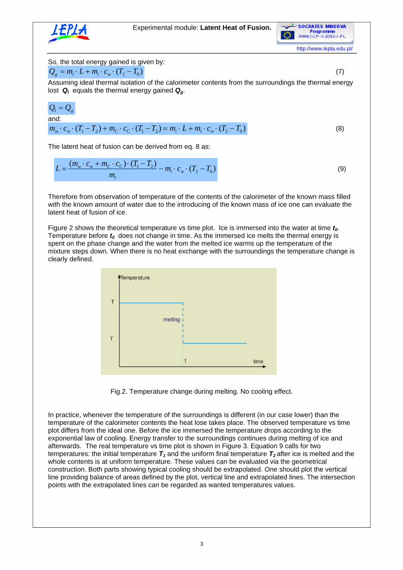
Therefore from observation of temperature of the contents of the calorimeter of the known mass filled with the known amount of water due to the introducing of the known mass of ice one can evaluate the latent heat of fusion of ice. Figure 2 shows the theoretical temperature vs time plot. Ice is immersed into the water at time t0. Temperature before t0 does not change in time. As the immersed ice melts the thermal energy is spent on the phase change and the water from the melted ice warms up the temperature of the mixture steps down. When there is no heat exchange with the surroundings the temperature change is clearly defined.

Fig.2. Temperature change during melting. No cooling effect. In practice, whenever the temperature of the surroundings is different (in our case lower) than the temperature of the calorimeter contents the heat lose takes place. The observed temperature vs time plot differs from the ideal one. Before the ice immersed the temperature drops according to the exponential law of cooling. Energy transfer to the surroundings continues during melting of ice and afterwards. The real temperature vs time plot is shown in Figure 3. Equation 9 calls for two temperatures: the initial temperature T1 and the uniform final temperature T2 after ice is melted and the whole contents is at uniform temperature. These values can be evaluated via the geometrical construction. Both parts showing typical cooling should be extrapolated. One should plot the vertical line providing balance of areas defined by the plot, vertical line and extrapolated lines. The intersection points with the extrapolated lines can be regarded as wanted temperatures values.


4

Fig.3. Temperature change during melting. Continuous cooling effect. APPARATUS FOR THE EXPERIMENTAL EXPLORATION. Temperature data are collected in the simple setup consisting of aluminium calorimeter and electromagnetic stirrer see fig. 4. The standard semiconductor temperature probe immersed in the calorimeter vessel records temperature of its contents. The calorimeter minimizes heat exchange with the surroundings while stirrer provides uniformity of the temperature within the volume of the calorimeter content. Measurements of masses of water and calorimeter are measured by laboratory balance.

Fig.4. Calorimeter

Experiment uses: i. aluminium calorimeter with housing ii. electromagnetic stirrer iii. laboratory balance (up to 200grams) iv. hot water (100grams) v. pieces of ice (approx. 20 grams) vi. Calculator Based Laboratory unit CBL: http://www.vernier.com/legacy/cbl/index.html

or CBL2: http://education.ti.com/us/product/tech/datacollection/features/cbl2.html vii. Temperature probe (standard CBL) viii. Graphic calculator TI83, TI83 Plus, TI 83 Plus SE, TI 84


5

ix. unit-to unit cable (standard). x. Program: LHEATF,– available for download at: http://www.lepla.edu.pl/ xi. TI-GRAPH LINK TM (optional) cable

http://education.ti.com/us/product/accessory/connectivity/features/cables.html#serialwin and software http://education.ti.com/us/product/accessory/connectivity/down/downgraph.html

xii. Personal computer with TI ConnectTM software (optional) Description: http://education.ti.com/us/product/accessory/connectivity/features/software.html

Download: http://education.ti.com/us/product/accessory/connectivity/down/download.html

Practical notes about the apparatus setup. - The Temperature probe should be connected to the channel CH1 of the CBL unit. - The water initial temperature should be approximately 10 - 20 degrees above the room

temperature. - Ice should be kept for some time outside fridge to warm it up to the melting point. - The temperature probe should be all the time plunged in the water contents of the calorimeter. - The calorimeter lid should be all the time in place to keep the thermal insulation of the calorimeter

vessel. - The electromagnetic stirrer should be turned on during the experiment in order to provide uniform

temperature within the water contents of the calorimeter. DATA ACQUISITION (TI 83)

In the experiment the temperature probe measures temperature of the water contents of the calorimeter vessel as a function time. The temperature changes due to the heat lose in favor of the surroundings of lower temperature as well as the thermal energy spent on the phase change of the ice immersed into the calorimeter. The auxiliary measurements of masses are to be performed giving value of the mass of the calorimeter’s vessel, mass of water and ice. The temperature measurements are controlled by means of the preloaded calculator program LHEATF. Program analyses the rate of change of the temperature and records temperature data only when the temperature relative change with respect to the last recorded value overcomes assumed value. So, the sampling time is self adjustable on the basis of the rate-of-change sensitive feedback . Experimental procedure is divided into the preparatory part and the data acquisition. Preparation: • Weigh the empty calorimeter vessel and stirrer accurately using laboratory balance. Record the

mass value mC. Note the material of which the calorimeter is made. • Pour in pure water (distilled, if available) to fill the calorimeter vessel in half of its volume. • Weigh accurately the calorimeter vessel (with stirrer) filled with water. • Calculate the mass of water in the calorimeter - mw. • Warm the calorimeter vessel up to the temperature between 40 and 50 oC. Use the laboratory

electric heater for this purpose. Alternatively you may fill in the calorimeter with the warm water and weigh it.

• Put the vessel into the calorimeter housing and cover it with the lid. • Immerse the temperature probe into the vessel. The end of the probe should be submerged in the

water! • Connect the temperature probe with the CBL and the CBL with the calculator. • Turn on the calculator and the CBL.


6

Data collection

1. Launch the program LHEATF by choosing its name from the PRGM menu. 2. Choose option 1: COLLECT DATA from the main menu- Fig.5 3. Introduce the expected minimum and maximum temperatures of the calorimeter content when

prompted. These values will be used for window range and are not critical for data collection. 4. Introduce the time duration of the observation ins seconds when prompted. As the observation

concerns the heat exchange with the surroundings before and after the phase transition the time value should be several minutes (5-15 min).

5. Introduce the time step in seconds when prompted. This value concerns the time interval between subsequent temperature measurements. As the temperature of the water during the phase transition changes quickly the sampling time should be several seconds (5-15sec).

6. Introduce the reference rate of temperature change R when prompted. R is defined by relative change of the subsequent temperature values – eq. 10.

n

nn

TTT

R−

= +1 (10)

The R value is used by the program LHEATF for recording or excluding the collected data point. Only those data points for which R is bigger than the reference value will be recorded. This self feedback mechanism saves the calculators memory. The reference R value should not be bigger than 0.02 – see Fig.6.

7. Check the position of the temperature probe and start data collection by pressing [ENTER]. 8. Observe the displayed plot. The plot will be updated as the temperature slowly drops as a result

of heat lose to the surrounding – Fig. 7. 9. Prepare several pieces of ice with the size that fits the inlet of the calorimeter. Leave it for a

while after taking it out from the freezer. 10. When approx. half of the chosen total time passes drop the ice into the calorimeter. Observe

the dramatic change of the temperature as the ice melts and the developed water absorbs heat - Fig. 8.

11. Data collection continues according to the defined total time of observation. When the time passes the final plot is displayed – Fig.9.

12. Finish observation choosing Quit option from main program menu.

Fig.5. Fig.6.

Fig.7. Fig.8.


7

13. Collected data are stored in a calculator’s memory as displayed – Fig. 10. and you can proceed using the standard calculator’s functions. Now you can disconnect the CBL from the calculator.

14. Weigh the calorimeter vessel again. Calculate the mass of the ice – mi. DATA ANALYSIS (TI83)

Further analysis can be performed using tools implemented in calculators (or other analytical software tools such as MS Excel spreadsheet). Collected data are stored in the calculator’s lists - Fig.10: - Time values t in seconds - List L1 - Temperature T values in [oC] - List L2 Program LHEATF creates copies if the collected data and stores them in the two pairs of the auxiliary lists: I pair: time values t in seconds - List L3 ; temperature T values in [oC] - List L4 II pair: time values t in seconds - List L5 ; temperature T values in [oC] - List L6 These lists will be used for the graphical analysis while the original data are safely kept in the lists L1 and L2.

Exemplary data are available for a download in the following calculator type files:

- Time values t in seconds as the files: Data sample/TI83/ L1 Data sample/TI83/ L3 Data sample/TI83/ L5

- Temperature T values in [oC] as the files

Data sample/TI83/ L2 Data sample/TI83/ L4 Data sample/TI83/ L6

Determination of the temperatures. Calculation of the latent heat of fusion upon the equation 9 requires values of the initial temperature of the water and calorimeter T1 just before the phase transition starts and the final temperature T2 after ice is melted and the whole calorimeter’s contents is at uniform temperature. Due to the process of continue heat exchange with the surrounding the observed temperature vs time plot ( Fig. 9) differs from the theoretical one – Fig. 2. Temperatures T1 and T2 can be established from the experimental plot by the geometrical interpolation method as shown on the Fig. 3. The collected data plot should be divided into three parts. First one representing cooling that precedes the phase change; second related to the melting and warming up the water developed from the ice; third part representing slow cooling of the final contents of the calorimeter.

Fig.9. Fig.10.


8

In the TI83 calculator this separation can be performed by selecting the data range on the separately defined plots. This can be done using pairs of the auxiliary lists: L3, L4, L5, L6, presented on separate plots. Separating the initial cooling curve.

1. Define the PLOT2 to present L3 vs L4 dependence – Fig.11. 2. Use Select function from the [2nd] [LIST] menu options – Fig.12. and fill in the names of the

lists as arguments – Fig. 13. 3. Point out the left and right bound of the data which you want to preserve from the first part of

the plot – Fig.14. 4. As the result the data lists are modified and selected part of data is plotted – Fig. 15.

Extrapolating the initial cooling curve.

1. Assuming the exponential character of cooling the exponential regression should be used from the [STAT] [CALC] menu option – Fig. 16.

2. The names of lists should be introduced as the arguments of the ExpReg function, together with the name of the function variable Y1 storing the regression equation – Fig. 17. The parameters of the established regression function are displayed – Fig. 18.

3. Now one can compare the experimental data and regression curve on one plot – Fig. 19.

Fig.11 Fig.12 Fig.13

Fig.14 Fig.15

Fig.16 Fig.17


9

In a similar way the final cooling curve can be separated and extrapolated from data stored in lists L5 vs L6 . The regression function for that part of the plot is stored in function Y2 and plotted on the Plot3 – Fig. 20. Now original data and established regression functions can be displayed on the same plot (activate Plot1) – Fig. 21. Interpolating the temperatures Temperatures T1 and T2 can be established from the plot by plotting the vertical line providing the balance of areas defined by the plot and the extrapolation curves (compare Fig.3.) 1. Select the central part of the plot using the ZBox option from the ZOOM menu – Fig.22,23, 24.

2. Use the option from the [DRAW] menu to draw the vertical line on the displayed plot – Fig. 25. 3. Adjust position of the line to obtain equal areas defined by the plot, vertical line and regression

curves – Fig. 26.

Fig.18 Fig.19

Fig.20 Fig. 21

Fig.22 Fig.23 Fig. 24

Fig.25 Fig.26


10

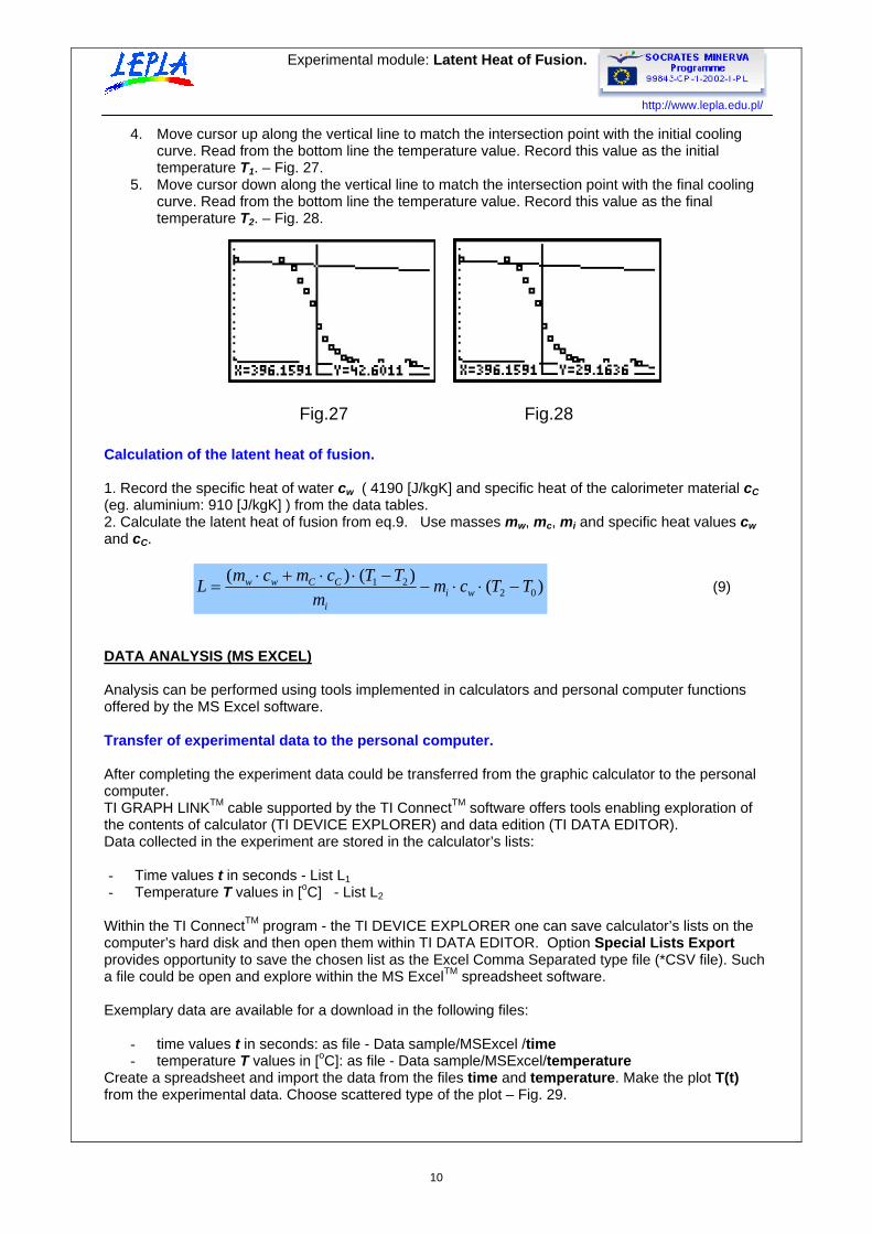
4. Move cursor up along the vertical line to match the intersection point with the initial cooling curve. Read from the bottom line the temperature value. Record this value as the initial temperature T1. – Fig. 27.

5. Move cursor down along the vertical line to match the intersection point with the final cooling curve. Read from the bottom line the temperature value. Record this value as the final temperature T2. – Fig. 28.

Calculation of the latent heat of fusion. 1. Record the specific heat of water cw ( 4190 [J/kgK] and specific heat of the calorimeter material cC (eg. aluminium: 910 [J/kgK] ) from the data tables. 2. Calculate the latent heat of fusion from eq.9. Use masses mw, mc, mi and specific heat values cw and cC.

)()()(02

21 TTcmm

TTcmcmL wii

CCww −⋅⋅−−⋅⋅+⋅

= (9)

DATA ANALYSIS (MS EXCEL)

Analysis can be performed using tools implemented in calculators and personal computer functions offered by the MS Excel software. Transfer of experimental data to the personal computer. After completing the experiment data could be transferred from the graphic calculator to the personal computer. TI GRAPH LINKTM cable supported by the TI ConnectTM software offers tools enabling exploration of the contents of calculator (TI DEVICE EXPLORER) and data edition (TI DATA EDITOR). Data collected in the experiment are stored in the calculator’s lists: - Time values t in seconds - List L1 - Temperature T values in [oC] - List L2

Within the TI ConnectTM program - the TI DEVICE EXPLORER one can save calculator’s lists on the computer’s hard disk and then open them within TI DATA EDITOR. Option Special Lists Export provides opportunity to save the chosen list as the Excel Comma Separated type file (*CSV file). Such a file could be open and explore within the MS ExcelTM spreadsheet software. Exemplary data are available for a download in the following files:

- time values t in seconds: as file - Data sample/MSExcel /time - temperature T values in [oC]: as file - Data sample/MSExcel/temperature

Create a spreadsheet and import the data from the files time and temperature. Make the plot T(t) from the experimental data. Choose scattered type of the plot – Fig. 29.

Fig.27 Fig.28


11

Fig. 29. Temperature vs time. Determination of the temperatures. Calculation of the latent heat of fusion upon the equation 9 requires values of the initial temperature of the water and calorimeter T1 just before the phase transition starts and the final temperature T2 after ice is melted and the whole calorimeter’s contents is at uniform temperature. Due to the process of continue heat exchange with the surrounding the observed temperature vs time plot ( Fig. 9) differs from the theoretical one – Fig. 2. Temperatures T1 and T2 can be established from the experimental plot by the geometrical interpolation method as shown on the Fig. 3. The collected data plot should be divided into three parts. First one representing cooling that precedes the phase change; second related to the melting and warming up the water developed from the ice; third part representing slow cooling of the final contents of the calorimeter. In the MS Excel this separation must be performed by selecting the data range in the series of data. Extrapolating the initial and final cooling curve.

1. Define the new scattered plot with the data range for the initial cooling curve as first series of data.

2. The data points well match the exponential curve so, one can apply the exponential regression model by adding the trend line(exponential type) to the plot. The trend line is drawn and resulting expression is displayed in the plot – Fig. 30- upper curve.

3. In a similar way the data range for the final cooling curve can be selected as second series of data.

4. The exponential trend line can be added to the plot and the respective expression is displayed in the plot – Fig. 30 – lower curve.

5. The central part of data should be used for defining the third series of data presented on the plot.

Interpolating the temperatures Temperatures T1 and T2 can be established from the plot by adjusting the vertical line providing the balance of areas defined by the plot and the extrapolation curves (compare Fig.3.)

1. Estimate from the plot the time value coordinate for the vertical line. Put this value as the reference value in a separate cell of the spreadsheet.

2. Define the vertical line (T ( t ) by two pairs of coordinates. The column representing time values should be defined as equal to the contents of the reference cell. The two temperature coordinates should excess the range of the observed temperatures.

Temperature change in time

25

30

35

40

45

50

0 200 400 600 800 1000time (sec)

temperature (oC)


12

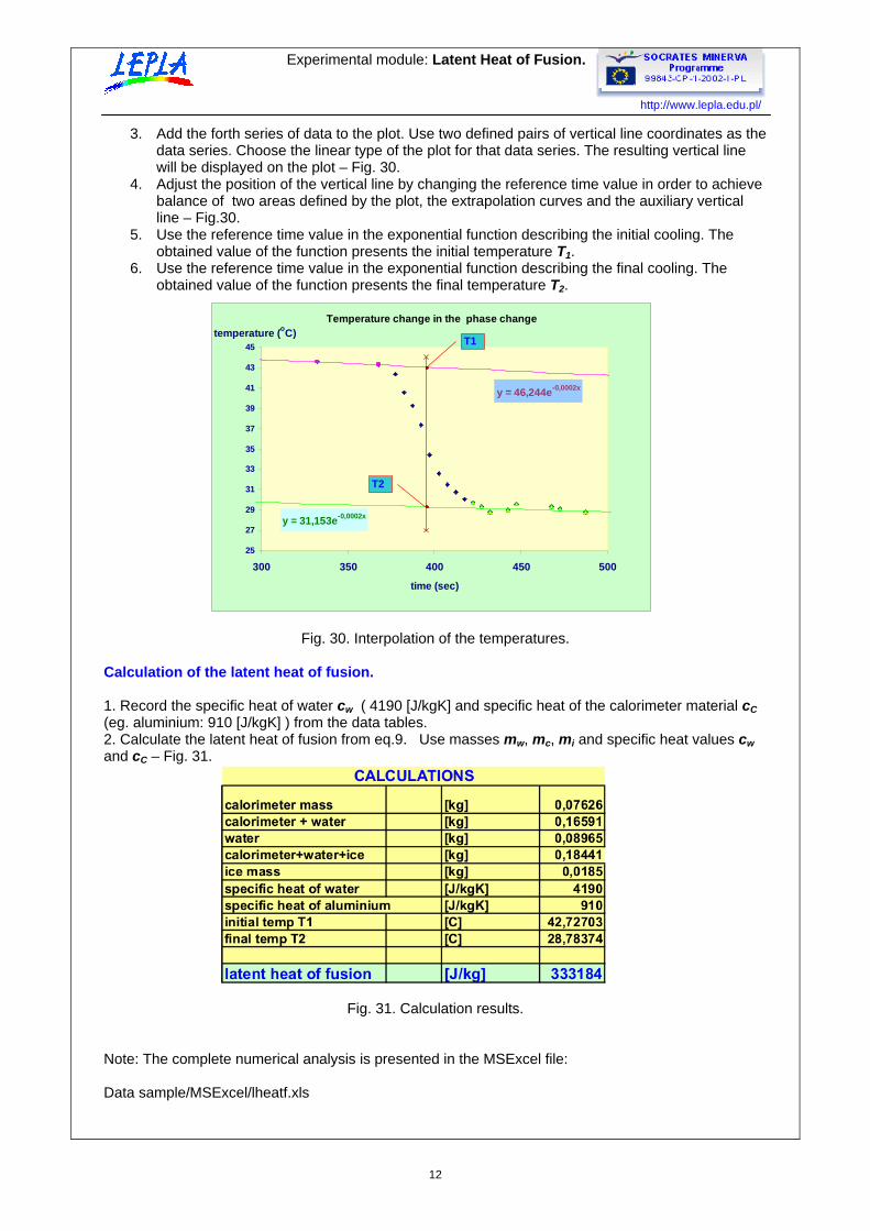
3. Add the forth series of data to the plot. Use two defined pairs of vertical line coordinates as the data series. Choose the linear type of the plot for that data series. The resulting vertical line will be displayed on the plot – Fig. 30.

4. Adjust the position of the vertical line by changing the reference time value in order to achieve balance of two areas defined by the plot, the extrapolation curves and the auxiliary vertical line – Fig.30.

5. Use the reference time value in the exponential function describing the initial cooling. The obtained value of the function presents the initial temperature T1.

6. Use the reference time value in the exponential function describing the final cooling. The obtained value of the function presents the final temperature T2.

Fig. 30. Interpolation of the temperatures.

Calculation of the latent heat of fusion. 1. Record the specific heat of water cw ( 4190 [J/kgK] and specific heat of the calorimeter material cC (eg. aluminium: 910 [J/kgK] ) from the data tables. 2. Calculate the latent heat of fusion from eq.9. Use masses mw, mc, mi and specific heat values cw and cC – Fig. 31.

Fig. 31. Calculation results. Note: The complete numerical analysis is presented in the MSExcel file: Data sample/MSExcel/lheatf.xls

Temperature change in the phase change

y = 46,244e-0,0002x

y = 31,153e-0,0002x

25

27

29

31

33

35

37

39

41

43

45

300 350 400 450 500

time (sec)

temperature (oC)T1

T2

Latent Heat of Fusion - LEPLA

Documents

Transcript of Latent Heat of Fusion - LEPLA