LATENT CLASS ANALYSIS OF RESIDENTIAL AND WORK …€¦ · LATENT CLASS ANALYSIS OF RESIDENTIAL AND...

-i-

LATENT CLASS ANALYSIS OF RESIDENTIAL

AND WORK LOCATION CHOICES

DRAFT FINAL REPORT

Prepared by:

Principal Investigator

Sabya Mishra, Ph.D., P.E.

Assistant Professor, Dept. of Civil Engineering, University of Memphis,

112D Engr. Sc. Bldg., 3815 Central Avenue, Memphis, TN 38152

Tel: 901-678-5043, Fax: 901-678-3026, Email: [email protected]

Co-Principal Investigators

Mihalis M. Golias, Ph.D. A.M. ASCE

Associate Professor, Dept. of Civil Engineering,

Associate Director for Research Intermodal Freight Transportation Institute,

University of Memphis, 104C Engr. Sc. Bldg., 3815 Central Avenue, Memphis, TN 38152,

Tel: 901-678-3048, Fax: 901-678-3026, Email: [email protected]

Rajesh Paleti, Ph.D.

Assistant Professor, Dept. of Civil & Environmental Engineering,

Old Dominion University, 135 Kaufman Hall, Norfolk, VA 23529

Tel: 757-683-5670, Email: [email protected]

Research Assistants

Afrid A. Sarker

Research Assistant, Dept. of Civil Engineering, University of Memphis,

302A Engineering Admin. Bldg., 3815 Central Avenue, Memphis, TN 38152

Phone: 260-797-1886, Email: [email protected]

Khademul Haque

Research Assistant, Dept. of Civil Engineering, University of Memphis,

302A Engineering Admin. Bldg., 3815 Central Avenue, Memphis, TN 38152

Phone: (860) 617-1489, Email: [email protected]

mailto:[email protected]





-ii-

DISCLAIMER

This research was funded by the Tennessee Department of Transportation (TDOT) in the

interest of information exchange. The material or information presented / published /

reported is the result of research done under the auspices of the Department. The content

of this presentation/publication/report reflects the views of the authors, who are

responsible for the correct use of brand names, and for the accuracy, analysis and any

inferences drawn from the information or material presented/published/reported. TDOT

assumes no liability for its contents or use thereof. This presentation/ publication/report

does not endorse or approve any commercial product, even though trade names may be

cited, does not reflect official views or policies of the Department, and does not constitute

a standard specification or regulation of the TDOT.

-iii-

TABLE OF CONTENTS

CHAPTER 1: BACKGROUND ........................................................................................ 7

CHAPTER 2: LITERATURE REVIEW ........................................................................... 10

2.1 Endogenous Market Segmentation ...................................................................... 12

2.2 Choice Set Variation ............................................................................................ 13

2.3 Heterogeneous Decision Rules ........................................................................... 13

2.4 Alternate Dependency Pathways ......................................................................... 14

CHAPTER 3: METHODOLOGICAL FRAMEWORK ...................................................... 15

3.1 Neighborhood Choice Component ....................................................................... 16

3.2 Conditional Zonal Destination Choice Component .............................................. 18

3.3 Sampling Destination Zones ................................................................................ 19

CHAPTER 4: CASE STUDY ......................................................................................... 20

4.1 Data Sources ....................................................................................................... 20

4.2 Data Assembly ................................................................................................ 21

4.3 Statistical Analysis ............................................................................................... 23

CHAPTER 5: RESULTS AND DISCUSSION ................................................................ 31

5.1 Neighborhood Choice Component ....................................................................... 31

5.1.1 Residential Neighborhood Choice ................................................................. 33

5.1.2 Work Neighborhood Choice .......................................................................... 34

5.2 Zonal Destination Choice Component ................................................................. 38

5.2.1 Zonal Residential Location Choice ................................................................ 38

5.2.2 Zonal Work Location Choice ......................................................................... 39

5.3 Estimation of Logsum .......................................................................................... 42

5.4 Elasticity Effects ................................................................................................... 42

CHAPTER 6: POTENTIAL APPLICATIONS OF PROPOSED LATENT CLASS MODELS

FOR LAND USE PLANNING ........................................................................................ 46

6.1 URBANSIM .......................................................................................................... 47

6.1.1 Overview ....................................................................................................... 47

6.1.2 Structure/Models ........................................................................................... 48

6.1.3 Data Inputs .................................................................................................... 49

-iv-

6.1.4 Model Outputs ............................................................................................... 49

6.1.5 Model Applications ........................................................................................ 49

6.2 PECAS ................................................................................................................ 51

6.2.1 Overview ....................................................................................................... 51

6.2.1 Structure/Models ........................................................................................... 51

6.2.2 Data Inputs .................................................................................................... 52

6.2.3 Model Outputs ............................................................................................... 52

6.2.4 Model Applications ........................................................................................ 52

6.3 Recommendation for improved land use planning for residential and workplace

location choices ......................................................................................................... 53

CHAPTER 7: CONCLUSION ........................................................................................ 54

APPENDIX A: OVERVIEW OF CASE STUDY DATA ................................................... 56

REFERENCES .............................................................................................................. 61

-v-

LIST OF TABLES

Table 5-1. Residential Neighborhood Choice: Multinomial Logit (MNL) Model ............. 32

Table 5-2. Residential Neighborhood Choice: Manski Model ........................................ 34

Table 5-3. Work Neighborhood Choice: MNL Model ..................................................... 36

Table 5-4. Work Neighborhood Choice: Manski Model ................................................. 37

Table 5-5: Summary comparison of Log-likelihood at convergence .............................. 38

Table 5-6. Zonal Residential and Work Location Choice Components ......................... 41

Table 5-7. Elasticity Effects of Residential Neighborhood Choice Model ...................... 44

Table 5-8. Elasticity Effects of Work Neighborhood Choice Model ............................... 45

LIST OF FIGURES

Figure 3-1. Conceptual framework of the proposed latent class model ......................... 16

Figure 4-1. Neighborhood Definition Based on Residential & Employment Density ...... 23

Figure 4-2. Commute distance- Age 18 to 24 years ...................................................... 24

Figure 4-3. Commute Distance: Work Flexibility ........................................................... 25

Figure 4-4. Commute distance: Gender ........................................................................ 25

Figure 4-5. Commute distance: Presence of child (0-5 years) ...................................... 26

Figure 4-6. Commute distance: Female and Presence of child (0-5 years)................... 27

Figure 4-7. Commute distance: Valid driver’s license ................................................... 28

Figure 4-8. Commute distance: Home owners .............................................................. 28

Figure 4-9. Commute distance: High Income ................................................................ 29

Figure 4-10. Commute distance: Auto ownership ......................................................... 30

Figure 6-1. URBANSIM Structure (Adapted from: Waddell, 2002) ................................ 50

Figure 6-2: PECAS Structure (Adapted from: HBA Specto Incorporated, 2007) ........... 53

Figure A-1. Distribution of schools in Nashville MPO area ............................................ 56

Figure A-2. Average school ratings in each TAZ ........................................................... 57

Figure A-3. K12 Students in each TAZ .......................................................................... 58

Figure A-4. Population: Age<17 years .......................................................................... 59

Figure A-5. High and Low-income category households ............................................... 60

-vi-

EXECUTIVE SUMMARY

Residential and work location choices are medium-to-long term decisions that have a

significant impact on day-to-day activity-travel decisions of people. Typically, these

choices are modeled using discrete choice models, but, several important aspects

including attitudes and preferences (e.g., greener lifestyle and tech-savvy attitude), the

consideration choice set, and the decision making mechanism are typically not observed

in the revealed preference dataset. These unobserved factors can lead to heterogeneity

in travel sensitivities across different population segments or lead to variation in the

consideration choice set across decision makers. Thus, standard choice models (e.g.,

MNL) cannot control for these factors. In such scenarios, latent class models that can

probabilistically classify households into latent classes (e.g., neo and conventional) are

particularly useful.

Since, location choices are usually undertaken at the zonal level (e.g., TAZ), the

size of choice set is typically large, comprising thousands of alternatives. While sampling

techniques can be used to resolve the computational problem associated with large

choice sets, the sampling mechanism itself might introduce some bias and make it more

difficult to identify latent segments. To avert this problem, this study proposes a two-stage

decision framework for location choices. In the first stage, a household (or a worker) is

assumed to select a neighborhood type (such as central business district, urban,

suburban) to live (or work). In the second stage, the household (or worker) is assumed to

choose a specific zone based on the selected neighborhood type. The latent class

analysis is undertaken at the first stage which has a much smaller choice set than the

conditional zonal choice model in the second stage. However, these two components are

not completely independent. Both the model components are estimated sequentially but

the expected utility or logsum from the zonal destination choice is used as an explanatory

variable in the neighborhood type choice alternatives to link the two model components.

For case study purposes, data from a 2012 household travel survey, conducted in

Nashville, Tennessee, is used. The model results indicate significant heterogeneity in the

consideration probability of different neighborhood type alternatives both in the residential

and work location choices. Also, the model applicability is tested by calculating elasticity

effects and identifying demographic groups with different residential and work location

preferences. Compared with standard MNL models, that assume all decision makers

consider the complete universal choice set, the latent class neighborhood models were

found to perform more strongly.

-7-

CHAPTER 1: BACKGROUND

Residential and work location choices are medium-to-long term decisions that have a

significant impact on day-to-day activity-travel decisions of people. These choices are

typically modeled using discrete choice models that assume certain decision making

mechanism. For instance, the Random Utility Maximization (RUM) rule is one such

mechanism in which the decision maker is assumed to choose the alternative that

provides the highest utility. Within the class of discrete choice models, the multinomial

logit (MNL) and its generalizations (e.g., nested logit, cross nested logit etc.) are

commonly used to analyze travel-related choices. In these models, the utilities of different

alternatives are specified as a function of different observed variables collected from

household survey data that can affect the choice being modeled. However, several

important aspects including the attitudes and preferences, the consideration choice set,

and the decision making mechanism are typically not observed in the survey data (Walker

and Li, 2006). For instance, it is reasonable to assume that there are certain

households/people who have greener life styles or tech-savvy attitudes from the rest of

the population. People in these ‘neo’ households are likely to have different residential

and work location preferences compared to those in ‘conventional’ households (Bhat and

Guo, 2007). But, these attitudinal variables are not available in most revealed preference

datasets. The effects of these unobserved factors can manifest in different ways. For

instance, these factors can lead to heterogeneity in travel sensitivities across different

population segments or lead to variation in the consideration choice set across decision

makers. So, standard choice models such as the MNL model cannot control for these

factors. In such scenarios, latent class models that can probabilistically classify

households into latent classes (e.g., neo and conventional) are particularly useful. It is

important to note that these groups or classes are not observed in the real world (and

hence the name ‘latent’).

Latent class choice models have been applied in various disciplines.

Methodological development and model application is spread over multiple domains

including marketing research (Dillon et al., 1994; Grover and Srinivasan, 1987; Russell

and Kamakura, 1993; Swait, 1994; Swait and Sweeney, 2000), economics (Boxall et al.,

-8-

n.d.; Boxall and Adamowicz, 2002), transportation (Walker and Li, 2006),

geography(Baerenklau, 2010; Hynes et al., 2008; Scarpa and Thiene, 2005), agriculture

(Mitani et al., 2008) and health science (Bandeen-Roche et al., 2006; Bucholz et al., 1996;

Jung and Wickrama, 2008; Lanza and Rhoades, 2011). Application of latent class models

in transportation planning can be summarized into four categories. First, studies that

focused on varying travel sensitivities and preferences where endogenous market

segmentations are made based on intrinsic biases and responsiveness to level-of-service

attributes (Bhat, 1998, 1997; Greene and Hensher, 2003). Recently, researchers also

started to explore attribute non-attendance where some respondents only consider a

subset of attributes during decision making (22). These studies can also be grouped

under the category of those dealing with varying travel sensitivity. Second, studies that

analyze the variation in consideration choice sets across decision makers (Manski, 1977;

Martínez et al., 2009). Third, studies that recognize that people might use alternate

decision making mechanisms or decision rules such as RUM or Random Regret

Minimization (RRM) while evaluating choice alternatives (Hess and Stathopoulos, 2013).

Fourth, studies that considered all possible dependency pathways while modeling

multiple choices simultaneously. For instance, work location decisions can be made

conditional on residential location or vice-versa leading to two different dependency

pathways (Waddell et al., 2007).

The current research belongs to the second group of studies that aim to uncover

population segments with varying choice sets in residential and work location choices.

Typically, location choices are undertaken at the zonal level (i.e., traffic analysis zone,

block, or parcel). The size of choice set in location choice models is typically large

extending into thousands of alternatives. Even with moderately sized choice sets, it is

difficult to identify more than 2-3 latent classes in most empirical applications. So, it can

be quite challenging to uncover latent classes with large choice sets. While researchers

have used sampling techniques to resolve the computational problem associated with

large choice sets, the sampling mechanism itself might introduce some bias and make it

further difficult to identify latent segments. To address this problem, the current study

adopted a two-stage decision framework for location choices. In the first stage, a

household (or a worker) will select a neighborhood (such as central business district,

-9-

urban, suburban etc.) to live (or work). In the second stage, the household (or worker) will

choose a specific zone conditional on the selected neighborhood in the first stage. The

latent class analysis is undertaken at the first stage which has a much smaller choice set

compared to the conditional zonal choice model in the second stage. For instance, certain

households might only consider high density neighborhoods while deciding where to

reside leading to varying consideration choice sets in the neighborhood choice model.

The two-stage modeling framework is also reasonable from a behavioral standpoint

because households are very unlikely to consider all zones within the study area while

making decisions regarding where to live and work. They are more likely to choose a

neighborhood and then explore residential choices within the neighborhood. However,

these two components are not completely independent. Better zonal alternatives within a

neighborhood should increase the likelihood of choosing that neighborhood over others.

This dependence between the neighborhood and zonal choice components is captured

by using log-sum from conditional zonal choice model as an explanatory variable in the

utility of the neighborhood choice model component.

The remainder of the report is organized as follows. A review of the relevant

literature is presented in the next section followed by the methodology. The case study

section (fourth section) describes the study area and data used for model development.

The results and discussion section (fifth section) provides insights on the case study

findings and possible application of the model and its results in transportation planning

and travel demand modeling. The sixth section explores potential applications of

proposed latent class models in modeling more efficient and accurate (residential/work)

location choices. The final section concludes the report and outlines the scope of future

research.

-10-

CHAPTER 2: LITERATURE REVIEW

As briefly discussed in the introduction section, the literature review is presented along

four themes to draw insights from past transportation research: (1) Endogenous market

segmentation; (2) choice set variation; (3) heterogeneous decision rules, and (4)

alternative dependency pathways. Before proceeding to specific segments, a broad

literature review is presented below.

Modern research on housing choice began with the study by Alonso, 1964, which

considers a city where employment opportunities are located in a single center (a

monocentric city). In Alonso’s study, the residential choice of households is based on

maximizing a utility function that depends upon the expenditure in goods, size of the land

lots, and distance from the city center. Several studies (Harris, 1963; Mills, 1972;

Wheaton, 1974) extended the work of Alonso by relaxing the assumption of a monocentric

city of employment opportunities. One of the most criticized aspects of these early

research works is that location is represented as a one-dimensional variable - distance

from the CBD. These models are therefore incapable of handling dispersed employment

centers and asymmetric development patterns (Waddell, 1996).

Even before Alonso’s, 1964 work, geographers and transportation planners had

developed the “gravity model” that provides a reasonable basis for the prediction of zone-

to-zone trips. Lowry applied the gravity model to residential location modeling in the well-

known Lowry Model. Specifically, Lowry assumed that retail trade and services are

located in relation to residential demand, and that residences are located in relation to

combined retail and basic employment. Workers are hypothesized to start their trips to

home from work, and distribute themselves at available residential sites according to a

gravity model, which attenuates their trips over increasing distance. This vital feature of

the Lowry model continues to dominate models of residential location in many practical

applications (Harris, 1996).

Another stream of research on modeling residential location is based on discrete

choice theory. In the context of residential location, the consumption decision is a discrete

choice between alternative houses or neighborhoods. The work by McFadden represents

the earliest attempt to apply discrete choice modeling to housing location. More recent

-11-

works using this approach include Gabriel and Rosenthal (1989), Waddell (1993, 1996),

and Ben-Akiva and Bowman (1998). As discussed next, these studies differ essentially in

their model structures, the choice dimensions modeled, the study region examined, and

the explanatory variables considered in the analysis.

The study by Gabriel and Rosenthal (1989) develops and estimates a multinomial

logit model of household location among mutually exclusive counties in the Washington,

D.C. metropolitan area. The findings indicate that race is a major choice determinant for

that area, and that further application of MNL models to the analysis of urban housing

racial segregation is warranted. Furthermore, the effects of household socio-demographic

characteristics on residential location are found to differ significantly by race. Waddell

(1993) examines the assumption implicit in most models of residential location that the

choice of workplace is exogenously determined. A nested logit model is developed for

worker’s choice of workplace, residence, and housing tenure for the Dallas-Fort Worth

metropolitan region. The results confirm that a joint choice specification better represents

household spatial choice behavior. The study also reaffirms many of the influences

posited in standard urban economic theory, as well as the ecological hypothesis of

residence clustering by socio-demographic status, stage of life cycle, and ethnicity.

In a later study, Waddell (1996) focuses on the implications of the rise of dual-

worker households. The choices of work place location, residential mobility, housing

tenure and residential location are examined jointly. The hypothesis is that home

ownership and the presence of a second worker both add constraints on household

choices that should lead to a combination of lower mobility rates and longer commutes.

The results indicate gender differences in travel behavior; specifically, the female work

commute distance has less influence on the residential location choice than the male

commute. Ben-Akiva and Bowman (1998) presented a nested logit model for Boston,

integrating a household’s residential location choice and its members’ activity schedules.

Given a residential location, the activity schedule model assigns a measure of

accessibility for each household member, which then enters the utility function in the

model of residential location choice. The results statistically invalidate the expected

decision hierarchy in which the daily activity pattern is conditioned on residential choice.

-12-

2.1 Endogenous Market Segmentation

Bhat (1997) recognized the need to accommodate differences in intrinsic mode biases

(preference heterogeneity) and differences in responsiveness to level-of-service

attributes (response heterogeneity) across individuals. He incorporated preference and

response heterogeneity into the MNL when studying mode choice behavior from cross-

sectional data in an intercity travel. The study found that endogenous segmentation model

described causal relationship best and provided intuitively more reasonable results

compared to traditional approaches (Bhat, 1997). Walker and Li (2006) conducted an

empirical study of residential location choices and uncovered three lifestyle segments –

suburban dwellers, urban dwellers, and transit riders with varying location preferences

(Walker and Li, 2006). Similarly, Wen and Lai (2010) demonstrated using air carrier

choice data that the latent class model outperforms the standard MNL model considerably

(Wen and Lai, 2010). Arunotayanun and Polak (2011) identified three latent segments in

the context of freight mode choice of shippers with three alternatives – small truck, large

truck, and rail as a function of several attributes including transport time, cost, service

quality and service flexibility (Arunotayanun and Polak, 2011). While the first segment

was found to be highly sensitive to all attributes considered, the second segment

preferred better service quality and the third segment preferred better service flexibility.

Wen et al. (2012) used a nested logit latent class model for high speed rail access in

Taiwan and showed that flexible substitution patterns among alternatives and preference

heterogeneity in the latent class nested logit model outperformed traditional models (Wen

et al., 2012). More recently, several studies analyzed attribute non-attendance which may

be considered as a variant of taste heterogeneity in which some respondents make their

choices based on only a subset of attributes that described the alternatives at hand

(Hensher, 2010). For example, it is possible that a portion of respondents do not care

about time savings while making travel decisions. Scarpa (2009) showed that 90% of the

respondents do not consider cost while choosing rock-climbing destination spots.

Similarly, Campbell et al. (2011) revealed that 61% of respondents are not attending to

cost while making environmental choices (Campbell et al., 2010). Hess and Rose (2007)

proposed a latent class approach to accommodate attribute non-attendance (Hess and

Rose, 2007), and a number of studies adopted similar approach thereafter (Hensher et

-13-

al., 2011; Hensher and Greene, 2009; Hess and Rose, 2007). Hess et al. (2012) suggest

that with this approach, different latent classes relate to different combinations of

attendance and non-attendance across attributes (Hess et al., 2012). Model estimation is

conducted to compute a non-zero coefficient, which is used in the attendance classes,

while the attribute is not employed in the non-attendance classes, i.e. the coefficient is

set to zero. In a complete specification, covering all possible combinations, this would

thus lead to 2𝐾 classes, with K being the number of attributes (Hess et al., 2012).

2.2 Choice Set Variation

Manski (1977) developed the theoretical framework for the two stage decision process

that accounts for choice set heterogeneity (Manski, 1977). Decision makers were

assumed to first construct their choice set in a non-compensatory manner and then make

choice conditional on the generated choice set using a compensatory mechanism (e.g.,

RUM). The choice probability of an alternative is obtained as a weighted probability of

choosing that alternative over all possible choice sets. Swait and Ben-Akiva (1987) and

Ben-Akiva and Boccara (1995) build on Manski’s framework and used explicit random

constraints to determine the choice set generation probability (Ben-Akiva and Boccara,

1995; Swait and Ben-Akiva, 1987). Bierlaire et al. (2009) stated that earlier latent class

choice set generation methods are hardly applicable to medium and large scale choice

problems because of the computational complexity that arises from the combinatorial

number of possible choice sets. If the number of alternatives in the universal choice set

is C, the number of possible choice sets is (2C − 1) (Bierlaire et al., 2009). Several

heuristics that derive tractable models by approximating the choice set generation

process were developed. The most promising heuristics are based on the use of penalties

of the utility functions, and were proposed by Cascetta and Papola (2001) and further

expanded by Martinez et al. (2009) (Cascetta and Papola, 2001; Martínez et al., 2009).

These heuristics were recently further modified to closely replicate the Manski’s original

formulation (Paleti, 2015).

2.3 Heterogeneous Decision Rules

An increasing number of studies investigated the use of alternatives to random utility

maximization (RUM) rule to explore which paradigm of decision rules best fits a given

dataset as well as the variation in decision rules across respondents. Srinivasan et al.

-14-

(2009) developed a latent class model that assigns respondents to either the utility

maximizing or disutility minimizing segments probabilistically for analyzing mode choice

decisions. This study found that only 32.5% respondents belong to the utility maximizing

segment whereas a majority (67.5%) belonged to the disutility minimizing segment

(Srinivasan et al., 2009). Along similar lines, Hess et al. (2013) developed latent class

models that linked latent character traits to choice of decision rule between RUM and

RRM. This found an almost even split between the shares of respondents that adopted

the two decision rules in the context of commute mode choice (Hess and Stathopoulos,

2013). Zhang et al. (2009) examined different types of group decision-making

mechanisms in household auto ownership choices using latent classes models (Zhang et

al., 2009).

2.4 Alternate Dependency Pathways

Joint choice modeling can result in several pathways of dependency among the choice

dimensions considered. However, one of the challenges is that as the number of choice

dimensions in the integrated modeling framework increases, the number of possible

dependency pathways among choice dimensions can explode very quickly. Specifically,

there are K! possible dependency structures in an integrated model with K choice

dimensions. So, it is not always possible to estimate latent models with all possible

dependency pathways. However, latent class models can be useful in empirical contexts

where there are very limited dependency pathways. For instance, Waddel et al. (2007)

used latent class models to estimate the proportion of households in which residential

location choice is made conditional on workplace location choice and vice versa (Waddell

et al., 2007). However, this study only considered single-worker households because of

several possible permutations of work and home location choices in multi-worker

households. Additionally, the authors also mention the complexity involved in modeling

the interdependencies when dynamics among choice dimensions can change over time.

In summary, latent class models have proven useful with better policy insights and

improved statistical fit in a wide array of empirical contexts within transportation.

Moreover, these models have the same data requirements as standard un-segmented

models. However, it might not be analytically tractable to estimate latent class models in

certain choice contexts without making some simplifying assumptions.

-15-

CHAPTER 3: METHODOLOGICAL FRAMEWORK

In this chapter, the methodology for identifying residential and work location choices at

neighborhood and zonal level is presented. Before proceeding with the methodology, we

present the nomenclature used throughout the report.

Nomenclature

Notation Description

q The decision-maker

i Neighborhood alternatives

C Universal choice set at neighborhood level

𝜙𝑞𝑖 Probability of decision maker q considers alternative i

𝑉𝑞𝑖 Observed utility experienced by q for alternative i

𝑿𝑞𝑖 Vector of explanatory variables

𝜀𝑞𝑖 Hidden utility experienced by q for alternative i

𝑈𝑞𝑖 Total utility experienced by q for alternative i

𝑉𝑞𝑠 Observed utility by q for each alternative for the zone s

𝑳𝑶𝑺𝑞,ℎ,𝑠 Level-of-service variables between home zone h, and work zone s

𝐷ℎ,𝑠 Distance between home zone h, and work zone s

𝑆𝑖𝑧𝑒𝑞𝑠 Size variable for destination zone s for decision maker q

𝒇(𝐷ℎ,𝑠) Vector of non-linear functions of 𝐷ℎ,𝑠

𝝅,𝜶, 𝜹 Coefficients

In this study, a two-stage decision making process is assumed in which the decision

maker (household for residential location choice and individual employee for work location

choice) first chooses the neighborhood in the first stage and then looks for a specific zone

within the chosen neighborhood in the second stage. Both these two model components

were estimated sequentially but the expected utility or logsum from the zonal destination

choice was used as an explanatory variable in the neighborhood choice alternatives to

link the two model components. Moreover, it is unlikely that all decision makers consider

the full set of neighborhoods while making the first stage neighborhood choice. This

variation in the consideration choice set of neighborhood choice is accounted using the

latent choice set Manski model. Lastly, the universal choice set of zonal choice conditional

-16-

on the neighborhood in the second stage comprises of all zones within the chosen

neighborhood of the decision maker. The size of this choice set can still be quite large.

So, importance sampling methods were used to construct the sampled choice set for

zonal choice in the second stage. A brief overview of different modeling components is

presented below. Let q be the index for the decision maker.

Figure 3-1. Conceptual framework of the proposed latent class model

3.1 Neighborhood Choice Component

Let i be the index for neighborhood alternative and 𝐶 denote the universal choice set of

the neighborhood choice 𝐶 = {1 = CBD, 2 = URBAN, 3 = SUBURBAN, 4 = RURAL}. It is

very likely that decision maker q only considers a subset 𝐶𝑞 (of C), known as the

consideration choice set, while making the actual choice. In the multinomial logit (MNL)

framework, the utility associated with alternative i can be written as:

𝑈𝑞𝑖 = 𝑉𝑞

𝑖 + 𝜀𝑞𝑖 = 𝜷𝑖

′𝑿𝑞𝑖 + 𝜀𝑞

𝑖 (1)

-17-

Where 𝑉𝑞𝑖 = 𝜷𝑖

′𝑿𝑞𝑖 is the observed part of the utility, 𝑿𝑞

𝑖 is the vector of explanatory

variables, and 𝜷𝑖 is the corresponding column vector of coefficients, and 𝜀𝑞𝑖 is standard

gumbel random variable that captures all unobserved factors that is independent and

identically distributed across alternatives and decision makers. The vector 𝑿𝑞𝑖 also

includes logsum from the conditional zonal destination choice model.

So, the probability of a decision maker q choosing an alternative ‘i’ from a set of mutually

exclusive and exhaustive alternatives 𝐶𝑞 is given by:

𝑃𝑞(𝑖|𝐶𝑞) =𝑒𝑉𝑞

𝑖

∑ 𝑒𝑉𝑞𝑗

𝑗∈𝐶𝑞

(2)

However, the consideration set 𝐶𝑞 is not observed by the analyst. To resolve this problem,

past researchers have assumed that observed choice is an outcome of two latent

(unobserved) steps – (1) formation of consideration set 𝐶𝑞 from the universal choice set

and (2) choice conditional on the consideration set 𝐶𝑞. So, the unconditional probability

that decision maker q chooses neighborhood i is obtained as a weighted average across

all possible consideration sets using Bayes’ theorem as follows (Manski, 1977):

𝑃𝑞(𝑖) = ∑ 𝑃𝑞(𝑖|𝐶𝑞) × 𝑃𝑞(𝐶𝑞)𝐶𝑞∈𝐶 (3)

The consideration set formation step of the Manski model is viewed as a non-

compensatory process whereas the second step is viewed as an outcome of

compensatory mechanism (in our case, this is the Random Utility Maximization (RUM)

principle in the MNL model). Consistent with this notion, the probability 𝜙𝑞𝑖 that decision

maker q considers alternative i is specified as a binary logit model as follows:

𝜙𝑞𝑖 =

𝑒𝜸𝑖′𝒁𝑞𝑖

1+𝑒𝜸𝑖′𝒁𝑞𝑖 (4)

where 𝒁𝑞𝑖 is the vector of variables that impact whether alternative i is considered by

decision maker q or not and 𝜸𝑖 is the corresponding column vector of coefficients. The

probability of different consideration sets can be computed using these individual

-18-

consideration probabilities. For instance, the probability of decision maker q considers the

choice set {CBD, URBAN} is given as follows:

𝑃𝑞[(𝐶𝐵𝐷,𝑈𝑅𝐵𝐴𝑁)𝑞] = 𝜙𝑞𝐶𝐵𝐷 × 𝜙𝑞

𝑈𝑅𝐵𝐴𝑁 × (1 − 𝜙𝑞𝑆𝑈𝐵𝑈𝑅𝐵𝐴𝑁) × (1 − 𝜙𝑞

𝑅𝑈𝑅𝐴𝐿) (5)

There are 15 possible consideration sets in the universal choice set comprising of four

alternatives – CBD, URBAN, SUBURBAN, and RURAL, excluding the null choice set

without any alternatives. However, all these subsets of alternatives are not intuitive from

a behavioral standpoint. For instance, {CBD, RURAL} is one such possible subset of

alternatives. However, it is difficult to justify why someone might consider both the

extreme neighborhoods (CBD and RURAL) that have very different residential and

employment composition but not intermediate options (URBAN and SUBURBAN). To

avoid such instances of behavioral inconsistency, we only considered the following 10

feasible consideration choice sets that avoid discontinuity: {CBD, URBAN, SUBURBAN,

RURAL}, {URBAN, SUBURBAN, RURAL}, {CBD, URBAN, SUBURBAN}, {CBD,

URBAN}, {URBAN, SUBURBAN}, {SUBURBAN, RURAL}, {CBD}, {URBAN},

{SUBURBAN}, {RURAL}.

Lastly, to ensure that the sum of probabilities across all alternatives in the universal choice

set add up to one, all the choice probabilities are re-scaled by the factor (1-probability of

all infeasible choice sets).

3.2 Conditional Zonal Destination Choice Component

Let s denote the index for location i.e. Traffic Analysis Zone (TAZ). The observed part of

the utility function for each alternative in the zonal choice set 𝑉𝑞𝑠 can be written as follows:

𝑉𝑞𝑠 = 𝐿𝑁(𝑆𝑖𝑧𝑒𝑞

𝑠) + 𝝅′𝑾𝑠 + 𝜶′ × 𝑳𝑶𝑺𝑞,ℎ,𝑠 + 𝜹′𝑓(𝐷ℎ,𝑠) (6)

where is 𝑆𝑖𝑧𝑒𝑞𝑠 the size variable for destination zone s for decision maker q (zonal household

population for residential location and industry-specific zonal employment for work

location), 𝑾𝑠 is vector of zonal variables describing zonal alternative s and 𝝅 is the

corresponding vector of coefficients, 𝑳𝑶𝑺𝑞,ℎ,𝑠 is the set of level-of-service variables between

zone pair (h,s) where h is the home zone and their interaction with decision maker

characteristics and 𝜶 is the corresponding vector of coefficients, 𝐷ℎ,𝑠 is the network distance

-19-

between home zone h and work zone alternative s, and 𝒇(𝐷ℎ,𝑠) is a vector of non-linear

functions of 𝐷ℎ,𝑠 (for example, linear, squared, cubic, and logarithmic) and 𝜹 is the

corresponding vector of coefficients. Please note that the last two components (LOS and

distance-based impedance measures) are relevant only to the work location component

where we assume that the home location is already known. Assuming i.i.d. standard

Gumbel term assumption for the unobserved part of utilities will lead to the MNL model.

3.3 Sampling Destination Zones

As mentioned earlier, it is computationally difficult to consider all location alternatives

within a neighborhood during model estimation. While a completely random sampling

approach will produce consistent parameter estimates, it is not an efficient option. So, a

sampling-by-importance model with TAZ activity-specific size terms (for both residential

and work location models) and a coefficient of -0.1 for “Distance between home and work

TAZ” variable (only for work location choice) was applied. During model estimation, a

correction term equal to

iqN

niln was added to the utility function of the sampled

alternative to account for the difference in the sampling probability and the frequency of

the alternative in the sample. The sampling correction term represents natural logarithm

of the ratio of the sampling frequency to selection probability for each alternative as was

substantiated in the theory (Ben-Akiva and Lerman, 1985; McFadden, 1978). In this

correction term, iq is the selection probability (probability to be drawn) which is a

function of size variable and simplified distance-based impedances, in is the selection

frequency in the sample or the number of times an alternative is chosen, and N is the

sample size (= 50 because we sample fifty TAZs).

-20-

CHAPTER 4: CASE STUDY

In this chapter, we present the data sets used and the steps performed to produce the

effective dataset needed for modeling and estimation purposes.

4.1 Data Sources

The data for this study is derived from the 2012 household travel survey data conducted

in Nashville metropolitan area. In addition to geo-coded location information, the data

include detailed socio-economic and demographic data and activity travel diary data of

all respondents. The travel skims and network related variables were gathered form the

Nashville Travel Demand Model (TDM). The following describes data collected for the

study:

▪ National Household Travel Survey (NHTS) data: The preliminary dataset

contained 5,164 households with 11,114 people and 5,682 of them were

employed. The NHTS serves as the nation's inventory of daily travel. Data is

collected on daily trips taken in a 24-hour period. It also includes:

– Household data on the relationship of household members, education level,

income, housing characteristics, and other demographic information

– Information on each household vehicle, estimates of annual miles traveled

– Data about drivers, including information on travel as part of work;

▪ Network Characteristics: Travel demand model was provided by the Nashville

MPO which included travel skims and network related variables.

▪ Socio-economic characteristics: NHTS data provided all the necessary socio-

economic characteristics used in this study.

▪ School ratings: Tennessee Department of Education maintains a rating scale using

Tennessee Value-Added Assessment System (TVAAS). It is a statistical method

used to measure the influence of a district or school on the academic progress

(growth) rates of individual students or groups of students from year-to-year. It

should be noted that, rating is available only for the public schools in the state of

TN.

-21-

4.2 Data Assembly

The first step in this stage was to geocode the work location coordinates in order to obtain

the work locations TAZs. Since the data was missing several key attributes, the following

approach is implemented (in order) to create a complete and effective dataset:

▪ Exclude records with missing work location coordinates or work location outside

the TAZ system

▪ Exclude records with missing information on any of the explanatory variables

▪ Exclude records where a person is employed in a zone where there is zero

employment in the corresponding industry

To construct the choice set for work location with 50 alternatives, 49 alternatives, different

from the observed work location, were randomly sampled. Once the 50 alternatives were

produced, for each individual, following tasks were performed:

▪ For each zonal pair (residential TAZ and potential work location TAZ), append

distance and logsum information.

▪ Append zonal employment information of the industry in which the person is

employed for all the sampled alternatives. For example, for a person employed in

the manufacturing industry, only manufacturing zonal employment must be used

▪ Append household and person explanatory variables to the estimation data set.

Some of the primary explanatory variables used in the model estimation are shown below:

Explanatory variables for household Explanatory variables for individual

Household Income Work Industry Housing Tenure (Own/Rent) Work hours (part-time/full-time) Presence of children Work Flexibility Household Auto ownership Educational Attainment Highest education attainment Gender Number of students per household Age Number of children per household Valid License Number of workers per household Student status (Part-time/Full-time) Number of disabled people per household

Instead of using the standard definition of spatial unit of location choices (census tract or

TAZ), this paper employs neighborhood categories based on household and employment

-22-

density to characterize location choices. This helps make the definition of choice

alternatives clear and manageable and more effectively captures the notion that people

are looking for a built environment (land use density) that suits their mobility and lifestyle

preferences. In other words, people are not choosing between TAZ A or B directly, but

rather between a unit that offers a built environment of certain attributes versus another

unit that offers a different built environment. Residence and workplace locations are

categorized into four possible alternatives or neighborhoods based on a combination of

population and employment density (population and employment in the half mile radius).

Only workers with work location outside home were considered in our analysis.

One of the key variables in the work location choice model is industry in which the worker

is employed. The Nashville travel demand model (TDM) uses work industry definition with

five categories – agriculture and mining, retail, manufacturing, transportation, and office.

The disaggregate work industry variable in the survey data was grouped together into

these five categories to be consistent with the regional TDM. Several explanatory

variables were considered in this study including age and gender composition, worker

characteristics, household income, educational attainment, housing type, housing tenure,

auto and bike ownership, typical commute mode choice and average daily trip frequency.

In addition, distance, auto travel time, transit availability, and transit generalized cost were

obtained from the network skims. Also, Hansen-type accessibility measures that indicate

a zone’s accessibility to different types of activity opportunities and mode choice log-sums

were calculated using zonal data and network skim files.

After extensive data cleaning, the final estimation sample includes 4,344

households and 3,992 employed individuals without any missing information on all

explanatory variables used in this study. The distribution of individuals in the four

residential neighborhood alternatives was - 8.90% rural, 29.74% suburban, 60.36%

urban, and 1.00% CBD as shown in Fig 4-1. The distribution of individuals with respect

to work neighborhood was 2.96% rural, 17.41% suburban, 65.88% urban, and 13.75%

CBD. In the final sample, the share of respondents who live in CBD was quite low. So,

the estimation of latent choice set model where people considered CBD alternative

probabilistically is difficult with such small sample size. So, respondents are assumed to

-23-

either consider or do not consider both the CBD and URBAN alternatives as a bundle but

not separately. So, the set of feasible choice sets is reduced to the six possibilities: {CBD,

URBAN, SUBURBAN, RURAL}, {CBD, URBAN, SUBURBAN}, {CBD, URBAN},

{SUBURBAN, RURAL}, {SUBURBAN}, {RURAL}. For the same reasons, the

SUBURBAN and RURAL alternatives are considered as bundle in the latent choice set

component of the work neighborhood choice model.

Figure 4-1. Neighborhood Definition Based on Residential & Employment Density

4.3 Statistical Analysis

This section gives an overview of how different socio-economic attributes affect the

commute distance, one of the crucial factor in work location choice.

Figure 4-2 suggests that young age group commute longer distances compared

to overall. A large fraction of them, about 9%, tend to travel 8-10 miles to work compared

to total aggregate of 6%. For larger distances, such as 34-36 miles, the difference is 4%

-24-

to 2.8%. This phenomenon can be explained by the fact that young age group are more

flexible when comes to work place location choice. At that age, commute distance is a

trivial factor when deciding where to work.

Figure 4-2. Commute distance- Age 18 to 24 years

Figure 4-3 shows how work flexibility affects the commute distance. Though, the

work flexibility has no significant effect for short commute distance, individuals with a job

with a provision of work flexibility tend to commute larger distance as the graph suggests.

It can be due to the reason that work flexibility is more appealing for the individuals and

hence s/he is willing to commute a few more miles to get the benefit.

Figure 4-4 shows the trend in commute distance for female individuals. It can be

observed that for shorter commute distance, less than 10 miles, there are less females

compared to others. But, for relatively larger distance such as 22-38 miles, there are more

females. This trend can be explained by the fact that women have less flexibility when

deciding on work locations which force them to commute larger distances in general.

0.00%

1.00%

2.00%

3.00%

4.00%

5.00%

6.00%

7.00%

8.00%

9.00%

10.00%

Distance (miles)

All Age 18 to 24

-25-

Figure 4-3. Commute Distance: Work Flexibility

Figure 4-4. Commute distance: Gender

0.00%

1.00%

2.00%

3.00%

4.00%

5.00%

6.00%

7.00%

8.00%

Distance (miles)

All Work Flexibility

0.00%

1.00%

2.00%

3.00%

4.00%

5.00%

6.00%

7.00%

8.00%

Distance (miles)

All Female

-26-

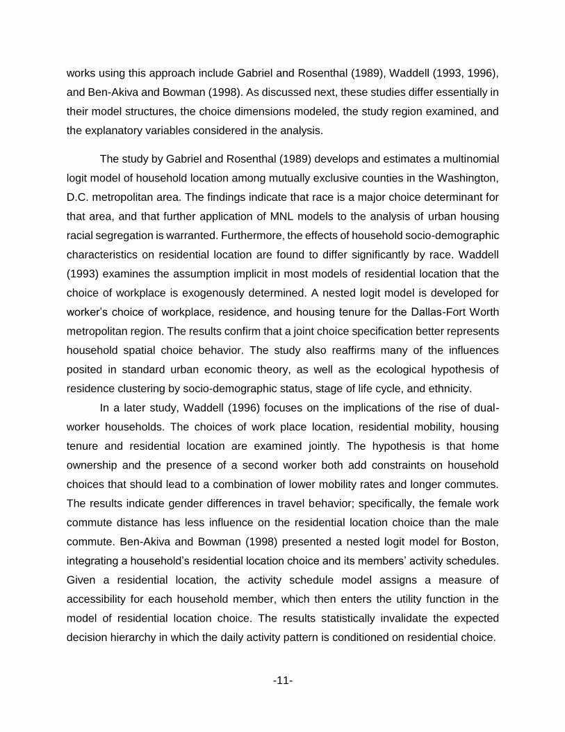
Figure 4-5 shows the relation between households with young children and

commute distance. It can be observed that a significant proportion of these households

prefer to live within 32 miles of work. There is also a fraction, about 10%, of these

households who commute more than 40 miles. This can be explained from the

perspective school’s location. Individuals with children tend to choose their residential

location based on school district which in some cases may be far away from their work

location. Hence, some people are forced to commute long way to work. But, nonetheless,

commute distance plays a significant role in workplace location choice.

Figure 4-5. Commute distance: Presence of child (0-5 years)

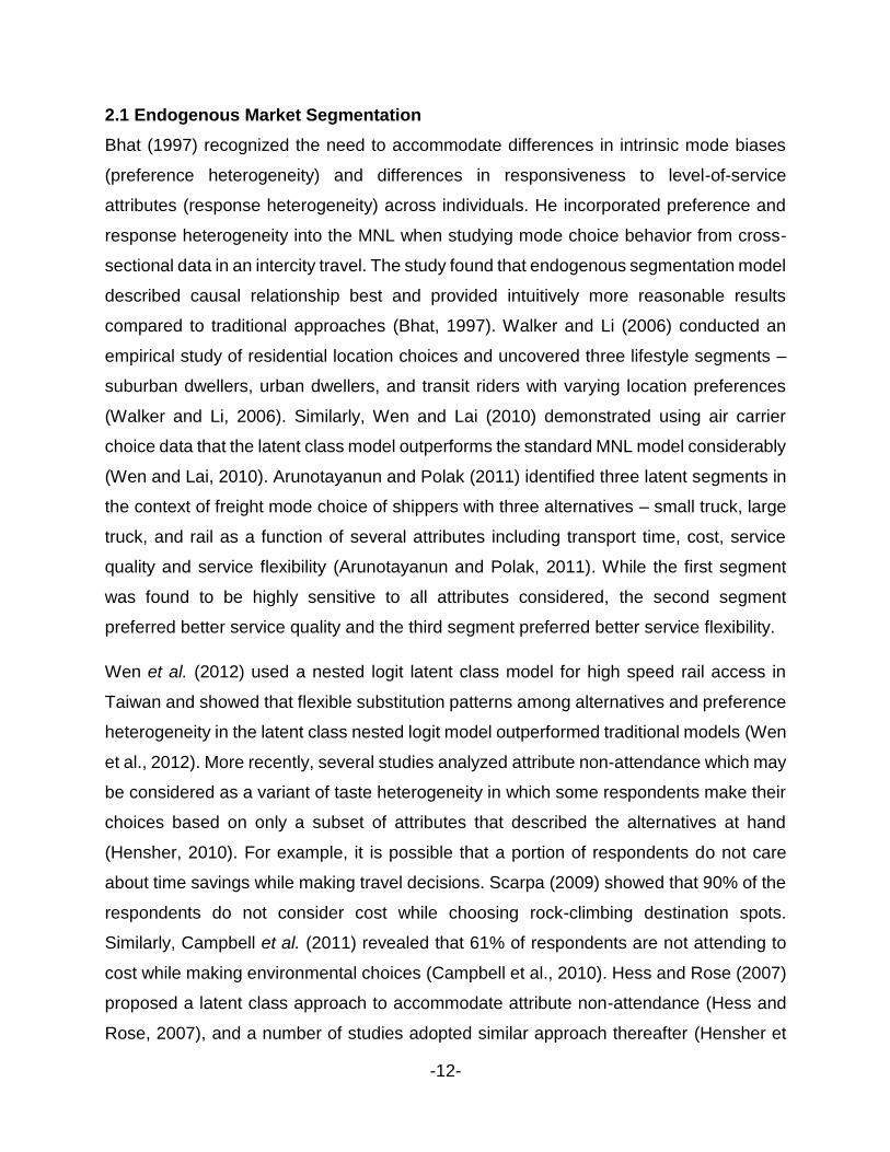
Figure 4-6 shows that female with young children prefer to live closer to home. A

very large fraction, about 8.3%, prefer to live within 6-8 miles of work and about 60% live

within 26 miles from work. When comparing with Fig 4-4 and 4-5, we can see that the

effect of “presence of children” is similar to the combined effect of “female with children”.

This trend is expected as mothers are the primary care giver for the young children and

because of the children’s school’s location, work locations closer to home are more

attractive.

0.00%

1.00%

2.00%

3.00%

4.00%

5.00%

6.00%

7.00%

8.00%

Distance (miles)

All POC

-27-

Figure 4-6. Commute distance: Female and Presence of child (0-5 years)

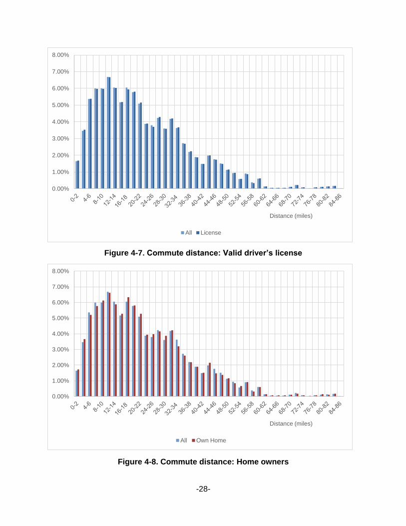
Figure 4-7 shows the relation between possession of valid driver’s license and

commute distance. It can be noticed that having a valid license doesn’t affect the

commute distance significantly. For almost any commute distance, these individuals are

comparable with others suggesting that individuals without a license commute as much

as the ones with license but underlines the fact that they are using other modes of

transportation.

Figure 4-8 shows the effect of home-ownership on commute distance. It can be

noticed that households who live in their owned-home are commuting more than the other

households by small extent. The figure shows that about 50% of these households

commute in the range of 4-22 miles. For larger commute distance they are comparable

with other households suggesting that they don’t prefer to commute more than 22 miles

in general. Also, home-ownership affects commute distance significantly because the

residential location tends to dictate the work location choice and hence factors such as

commute distance comes into play.

0.00%

1.00%

2.00%

3.00%

4.00%

5.00%

6.00%

7.00%

8.00%

9.00%

Distance (miles)

All Female & POC

-28-

Figure 4-7. Commute distance: Valid driver’s license

Figure 4-8. Commute distance: Home owners

0.00%

1.00%

2.00%

3.00%

4.00%

5.00%

6.00%

7.00%

8.00%

Distance (miles)

All License

0.00%

1.00%

2.00%

3.00%

4.00%

5.00%

6.00%

7.00%

8.00%

Distance (miles)

All Own Home

-29-

Figure 4-9 shows the relation between income and commute distance. It can be

noticed that high income households are commuting significantly more than the other

households. The figure shows that a large portion, about 22%, of these households

commute in the range of 16-24 miles. These households have less presence in the

categories between 10-16 miles suggesting that they usually commute more than 16

miles or less than 10 miles in general. Intuitively, we would expect the individuals in high-

income households to be trivially affected by the commuting distance.

Figure 4-9. Commute distance: High Income

Figure 4-10 shows the effect of auto-ownership on commute distance. It can be

noticed that households with 4 or more vehicles are commuting significantly more than

the other households. The figure shows that about 10% of these households commute

12-14 miles, 8% travel 30-32 miles and 6% commute more than 50 miles. These

households have less presence in the categories between 14-22 miles suggesting that

they usually commute more than 22 miles or less than 14 miles in general. Also,

commuting distance tends to have less effect on the individuals belonging to these type

of households when deciding on workplace locations.

0.00%

1.00%

2.00%

3.00%

4.00%

5.00%

6.00%

7.00%

8.00%

Distance (miles)

All High Income

-30-

Figure 4-10. Commute distance: Auto ownership

0.00%

2.00%

4.00%

6.00%

8.00%

10.00%

12.00%

Distance (miles)

All >=4 Vehicles

-31-

CHAPTER 5: RESULTS AND DISCUSSION

The location choice models comprise of two components – neighborhood choice and

zonal choice conditional on neighborhood. For brevity, only results of the final models are

presented in this study. For the Manski models with probabilistic choice sets, each

explanatory variable was tested both in the utility specification as well as the alternative

consideration probability specification for each alternative and the specification that

provided better data fit as chosen.

5.1 Neighborhood Choice Component

The CBD alternative was chosen as the reference alternative. Given that there are several

other variables in the model, the constants in the model do not have substantive

behavioral interpretation. Nonetheless, the relative magnitude of constants suggests that

people, on average, prefer URBAN, SUBURBAN, and RURAL neighborhoods (and in that

order) compared to CBD areas. Households with higher trip frequency are more likely to

reside in the URBAN and SUBURBAN regions of the study area. As expected,

households with children are more likely to reside in SUBURBAN and RURAL areas.

Interestingly, households with more jobs (i.e., workers) are less likely to live in URBAN

areas. Households with more female members are more inclined to reside in less dense

neighborhoods. Households with higher number of licensed drivers tend to live in the

suburban and rural neighborhoods. The high positive parameter estimates on single

family detached households show that these households almost certainly do not live in

CBD neighborhood. Households with zero vehicles are most likely group to live in the

CBD whereas households with more cars than driving age adults are more inclined to live

in less dense neighborhoods. Households with more than $75K income and higher

educational attainment (bachelor degree and higher) are less likely to reside in low

density neighborhoods.

Among the four alternatives, the two low density options – SUBURBAN and

RURAL were found to be considered probabilistically. Specifically, owner-occupied

households are more likely to consider SUBURBAN and RURAL households. Also, while

higher bicycle ownership levels are associated with higher likelihood of choosing

SUBURBAN neighborhood, it reduces the likelihood for RURAL neighborhood. This result

-32-

is probably indicative of inadequate bicycle and pedestrian infrastructure in RURAL areas.

As expected, households with higher average age are more likely to consider RURAL

neighborhood compared to relatively younger households.

Tables 5-1 to 5-4 present the results of the neighborhood choice components of

residential location and work location models respectively. For comparison purposes, a

multinomial logit model (MNL) model, that assumes that all households consider all the

four neighborhood options, was also estimated as shown in Table 5-1.

Table 5-1. Residential Neighborhood Choice: Multinomial Logit (MNL) Model

Variables Description Urban Sub-Urban Rural

(Base Alternative: CBD) Coeff. t-stat Coeff. t-stat Coeff t-stat

Constant 3.696 7.605 1.383 2.758 -1.471 -2.502

Children per household aged 6 to 10 years

0.342 3.621 0.573 3.637


0.409 2.715

Jobs per household -0.146 -3.451

Number of females per household 0.887 3.284 0.887 3.284 0.887 3.284

Number of licensed drivers per household

0.401 5.589 0.645 6.853

Average age per household 0.015 3.955

Residence type: single-family detached house

6.659 1.965 7.461 2.200 7.461 2.200

Household Residence Ownership: Owned/bought

0.549 4.582 1.011 4.437

Auto sufficiency: Zero vehicle -1.387 -3.126 -2.169 -4.254 -1.927 -2.966

Auto sufficiency: Category 1 -0.264 -1.838

Auto sufficiency: Category 3 0.356 3.892 1.166 9.397

Household income: More than $75K -0.989 -2.553 -0.771 -1.949 -1.056 -2.571

Number of bikes owned per household 0.634 1.541 0.634 1.541 0.634 1.541

Highest Education Attainment in household: Graduate Degree

-1.854 -3.776 -2.205 -4.422 -2.768 -5.360

Highest Education Attainment in household: Bachelor Degree

-1.273 -2.652 -1.570 -3.224 -1.727 -3.461

Number of Observations 4344

Number of Parameters Estimated 16

Mean log-likelihood at convergence -0.808

Log-likelihood -3509.719

-33-

5.1.1 Residential Neighborhood Choice

The positive magnitudes of the constants suggest that there is a baseline preference for

“Rural”-to-“Urban” neighborhoods for residential location choice. The model estimates

significantly suggest that households with increasing number of trips are more likely to

prefer “Urban” and “Sub-urban” neighborhood locations. The model also suggests that

households with children are more likely to choose “Sub-Urban” or “Rural” neighborhood

locations due to the presence of good schools in these neighborhood levels. Households

with higher number of jobs are less likely to choose “Sub-Urban” alternative than “CBD”.

This is intuitive since people with more jobs tend to remain extremely busy and they prefer

closest possible household locations from their work place which is more available in

“CBD” areas. Households with more number of female members are more likely to

choose between “Urban”, “Sub-Urban” and “Rural” neighborhood locations than “CBD”.

Households with higher number of licensed drivers have higher propensity to choose

between “Sub-Urban” or “Rural” locations. Households with zero auto sufficiency are less

likely to choose between the three alternatives than the base alternative, “CBD”. This is

because people without vehicles prefer transit for commuting and travelling and hence

they prefer “CBD” area for household locations where transit is more accessible. On the

other hand, people with higher auto sufficiency are more likely to select “Sub-Urban” or

“Rural” area since presence of a number of vehicles makes trip distance an insignificant

factor while travelling. Households with higher income and higher degrees are less likely

to choose from any of the 3 alternative than the “CBD” alternative since they prefer urban

and luxurious lifestyles and friendlier environment.

The log-likelihood of the MNL and Manski models are -3,509.7 and -3,502.1,

respectively. The Likelihood Ratio (LR) test statistic of comparison between the two

models is 19.30 that is significantly greater than 14.07 which is the critical chi-squared

value corresponding to 3 degrees of freedom at 95 percent confidence level. This

underscores the importance of accounting for latent choice sets in residential

neighborhood choices.

-34-

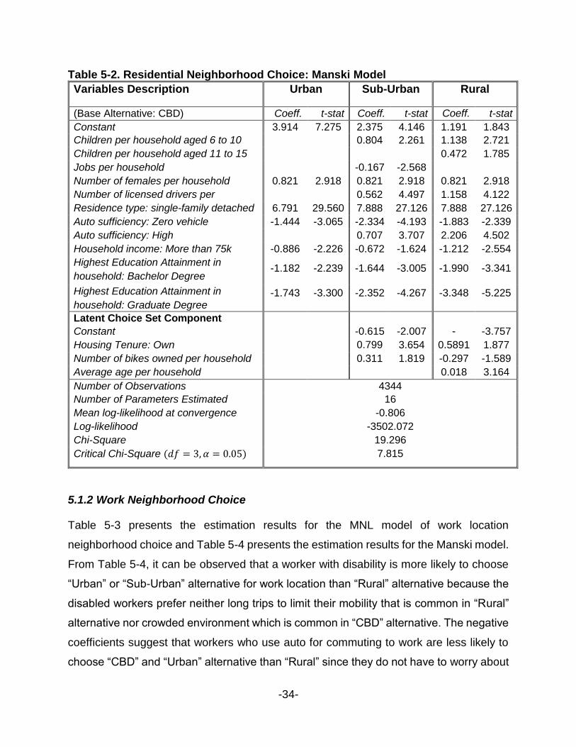
Table 5-2. Residential Neighborhood Choice: Manski Model

Variables Description Urban Sub-Urban Rural

(Base Alternative: CBD) Coeff. t-stat Coeff. t-stat Coeff.

t-stat

Constant

3.914 7.275 2.375 4.146 1.191 1.843

Children per household aged 6 to 10

years

0.804 2.261 1.138 2.721


years

0.472 1.785

Jobs per household

-0.167 -2.568

Number of females per household

0.821 2.918 0.821 2.918 0.821 2.918

Number of licensed drivers per

household

0.562 4.497 1.158 4.122

Residence type: single-family detached

house

6.791 29.560 7.888 27.126 7.888 27.126

Auto sufficiency: Zero vehicle

-1.444 -3.065 -2.334 -4.193 -1.883 -2.339

Auto sufficiency: High

0.707 3.707 2.206 4.502

Household income: More than 75k

-0.886 -2.226 -0.672 -1.624 -1.212 -2.554

Highest Education Attainment in

household: Bachelor Degree

-1.182 -2.239 -1.644 -3.005 -1.990 -3.341


household: Graduate Degree

-1.743 -3.300 -2.352 -4.267 -3.348 -5.225

Latent Choice Set Component

Constant

-0.615 -2.007 -

1.6117

-3.757

Housing Tenure: Own

0.799

1

3.654 0.5891 1.877

Number of bikes owned per household

0.311 1.819 -0.297 -1.589

Average age per household

0.018 3.164



Mean log-likelihood at convergence -0.806


Chi-Square 19.296

Critical Chi-Square (𝑑𝑓 = 3, 𝛼 = 0.05) 7.815

5.1.2 Work Neighborhood Choice

Table 5-3 presents the estimation results for the MNL model of work location

neighborhood choice and Table 5-4 presents the estimation results for the Manski model.

From Table 5-4, it can be observed that a worker with disability is more likely to choose

“Urban” or “Sub-Urban” alternative for work location than “Rural” alternative because the

disabled workers prefer neither long trips to limit their mobility that is common in “Rural”

alternative nor crowded environment which is common in “CBD” alternative. The negative

coefficients suggest that workers who use auto for commuting to work are less likely to

choose “CBD” and “Urban” alternative than “Rural” since they do not have to worry about

-35-

using any other form of transport and they have voluntary control over the distance and

time for travel. On the other hand, workers with flexible work schedule and working 5 days

a week are more likely to choose “CBD” and “Urban” alternative than “Rural”. The

negative coefficients suggest that workers working in agricultural sector are less likely to

choose between the 3 alternatives than “Rural” alternative which is very much intuitive

since most of the agricultural lands and working conditions are situated in rural areas.

This is similar with workers working in manufacturing and transportation sector since most

of the factories, highway and freeway construction and other road maintenance works are

mostly located in rural areas. On the other hand, workers working in office or performing

mostly desk jobs more likely prefer the “Urban” or “CBD” alternative which is intuitive.

Individuals with high school degrees tend to find jobs in “Sub-urban” alternative than

“Rural” whereas individuals with higher degrees less likely prefer “CBD” than “Rural”. It is

also interesting to observe that individuals with household neighborhood location choice

as “CBD” are more likely to prefer “CBD” alternative for work location choice whereas

individuals with “Urban” or “Sub-Urban” household neighborhood location alternative are

more likely to choose from the three alternatives than the base alternative, that is, “Rural”.

This is because individuals with “Urban” or “Sub-Urban” alternative usually have owned

residence which means they are looking for permanent settlements or have children.

Hence they prefer these alternative for work location due to friendlier environment, good

schools and country life.

The RURAL alternative was chosen as the reference alternative. Workers with

disability are more likely to be employed in the URBAN and SUBURBAN neighborhoods

compared to CBD and RURAL areas. This is intuitive because disabled workers do not

prefer longer trips typically associated with RURAL neighborhood as well as crowded

environment of CBD neighborhood. Workers who use auto mode for commute are less

likely to be employed in CBD and URBAN areas. On the other hand, workers who have

flexible work schedule and work five days a week are more likely to be employed in CBD

and URBAN neighborhoods. Industry type was found to have a strong impact on work

neighborhood choice. For instance, workers in agriculture, manufacturing, and

transportation industries are more likely to be working in RURAL neighborhood which is

consistent with the land use in these areas (e.g., agricultural land, factories, construction

-36-

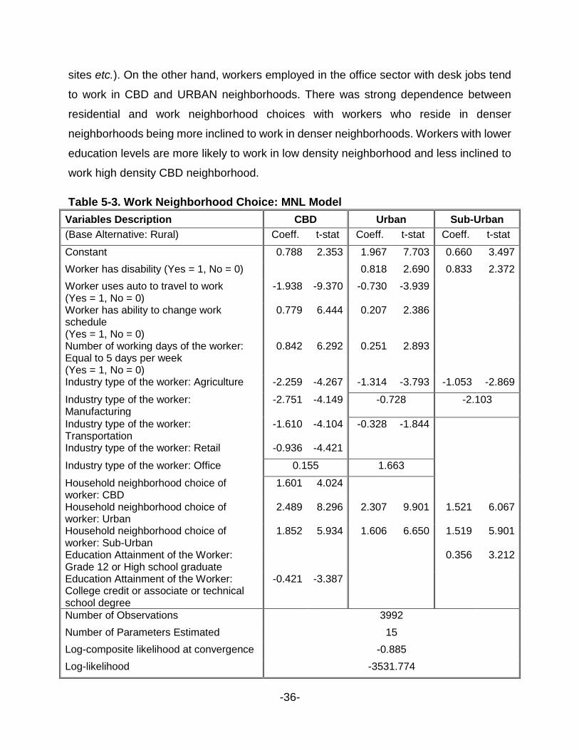
sites etc.). On the other hand, workers employed in the office sector with desk jobs tend

to work in CBD and URBAN neighborhoods. There was strong dependence between

residential and work neighborhood choices with workers who reside in denser

neighborhoods being more inclined to work in denser neighborhoods. Workers with lower

education levels are more likely to work in low density neighborhood and less inclined to

work high density CBD neighborhood.

Table 5-3. Work Neighborhood Choice: MNL Model

Variables Description CBD Urban Sub-Urban

(Base Alternative: Rural) Coeff. t-stat Coeff. t-stat Coeff. t-stat

Constant 0.788 2.353 1.967 7.703 0.660 3.497

Worker has disability (Yes = 1, No = 0) 0.818 2.690 0.833 2.372

Worker uses auto to travel to work (Yes = 1, No = 0)

-1.938 -9.370 -0.730 -3.939

Worker has ability to change work schedule (Yes = 1, No = 0)

0.779 6.444 0.207 2.386

Number of working days of the worker: Equal to 5 days per week (Yes = 1, No = 0)

0.842 6.292 0.251 2.893

Industry type of the worker: Agriculture -2.259 -4.267 -1.314 -3.793 -1.053 -2.869

Industry type of the worker: Manufacturing

-2.751 -4.149 -0.728 -2.103

Industry type of the worker: Transportation

-1.610 -4.104 -0.328 -1.844

Industry type of the worker: Retail -0.936 -4.421

Industry type of the worker: Office 0.155 1.663

Household neighborhood choice of worker: CBD

1.601 4.024

Household neighborhood choice of worker: Urban

2.489 8.296 2.307 9.901 1.521 6.067

Household neighborhood choice of worker: Sub-Urban

1.852 5.934 1.606 6.650 1.519 5.901

Education Attainment of the Worker: Grade 12 or High school graduate

0.356 3.212

Education Attainment of the Worker: College credit or associate or technical school degree

-0.421 -3.387



Log-composite likelihood at convergence -0.885


-37-

Table 5-4. Work Neighborhood Choice: Manski Model

Variables Description CBD Urban Sub-Urban

(Base Alternative: Rural) Coeff. t-stat Coeff. t-stat Coeff.

t-stat

Constant

-0.969 -2.155 0.141 0.349 0.668 3.471

Worker has disability (Yes = 1, No = 0)

0.815 2.616 0.868 2.241

Worker uses auto to travel to work

(Yes = 1, No = 0)

-2.348 -8.960 -1.148 -4.653

Worker has ability to change work

schedule

(Yes = 1, No = 0)

2.493 7.333 1.948 5.860

Number of working days:5 days per week

(Yes = 1, No = 0)

0.985 6.187 0.403 3.257

Industry type of the worker: Agriculture

-2.708 -4.574 -1.758 -4.293 -1.225 -3.368


-2.639 -3.736 -0.599 -1.603 -0.599 -1.603


-1.915 -4.046 -0.658 -1.973

Industry type of the worker: Retail

-0.966 -4.529

Education Attainment of the Worker:

Grade 12 or High school graduate

0.423 2.758

Education Attainment of the Worker:

College credit or associate or technical

school degree

-0.421 -3.433

Residential neighborhood choice: CBD

1.447 3.720

Residential neighborhood choice: Urban

2.903 8.995 2.781 10.332 1.504 5.918

Residential neighborhood choice: Sub-

Urban

1.925 5.813 1.727 6.326 1.504 5.778

Latent Choice Set Component

Constant

-0.320 -1.597 -0.320 -1.597

Worker has ability to change work

schedule

(Yes = 1, No = 0)

5.518 9.267 5.518 9.267


-0.530 -2.905 -0.530 -2.905



Log-composite likelihood at convergence -0.880


Chi-Square 41.094

Critical Chi-Square (𝑑𝑓 = 3, 𝛼 = 0.05) 7.815

Among the four alternatives, the two low density options – SUBURBAN and

RURAL were found to be considered probabilistically. But, as discussed earlier, these

alternatives were assumed to be considered as a bundle in the latent choice component

of the Manski model. Workers with flexible work schedule are more likely to consider

these low density neighborhoods compared to workers with fixed work schedule. Also,

-38-

workers employed in retail industrial sector are less likely to consider low density

neighborhoods in their work neighborhood choices. Again, the log-likelihood of the MNL

and Manski work neighborhood models are -3,531.8 and -3,511.2, respectively. The LR

test statistic of comparison between the two models is 41.09. This value is considerably

larger than 7.82 which is the critical chi-squared value corresponding to 3 degrees of

freedom at 95 percent confidence level. This indicates superior data fit in the Manski

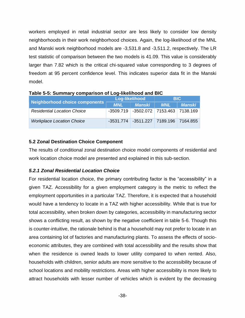
model.

Table 5-5: Summary comparison of Log-likelihood and BIC

Neighborhood choice components Log-likelihood BIC

MNL Manski MNL Manski

Residential Location Choice -3509.719 -3502.072 7153.463 7138.169

Workplace Location Choice -3531.774 -3511.227 7189.196 7164.855

5.2 Zonal Destination Choice Component

The results of conditional zonal destination choice model components of residential and

work location choice model are presented and explained in this sub-section.

5.2.1 Zonal Residential Location Choice

For residential location choice, the primary contributing factor is the “accessibility” in a

given TAZ. Accessibility for a given employment category is the metric to reflect the

employment opportunities in a particular TAZ. Therefore, it is expected that a household

would have a tendency to locate in a TAZ with higher accessibility. While that is true for

total accessibility, when broken down by categories, accessibility in manufacturing sector

shows a conflicting result, as shown by the negative coefficient in table 5-6. Though this

is counter-intuitive, the rationale behind is that a household may not prefer to locate in an

area containing lot of factories and manufacturing plants. To assess the effects of socio-

economic attributes, they are combined with total accessibility and the results show that

when the residence is owned leads to lower utility compared to when rented. Also,

households with children, senior adults are more sensitive to the accessibility because of

school locations and mobility restrictions. Areas with higher accessibility is more likely to

attract households with lesser number of vehicles which is evident by the decreasing

-39-

coefficients with respect to increasing number of vehicles. On the other hand, household

with high income enjoys higher utility compared to lower income households. Similarly,

household individuals with higher education levels tends to locate in areas with higher

accessibility.

The coefficient on the size variable – natural logarithm of the “total number of

households in the TAZ’ is fixed to one to ensure that individual destination zone

preferences sum up to zonal control totals. Accessibility to different types of employment

opportunities was found to a significant determinant of zonal residential location

decisions. To be specific, households are less likely to reside in zones with high

manufacturing accessibility which is expected given that these zones tend to have higher

pollution levels and limited infrastructure for recreational activities. Interestingly, owner-

occupied households tend to reside in areas with lower total employment accessibility

compared to rental households. On the other hand, households with more children and

senior adults prefer zones with better accessibility. Also, zones with higher total

employment accessibility attract households with lower auto ownership levels, higher

income, and higher educational attainment.

5.2.2 Zonal Work Location Choice

The workplace location choice components of the model suggest that an individual’s

decision or choice rely very significantly on the commuting distance and the morning peak

hour travel time. It is very intuitive that a particular TAZ is more likely to be chosen if it is

closer to one’s residential location. Among the commuting factors, presence of at least

one type of transit between residence and work was found to be crucial. This indicator

variable shows when there is at least a feasible mode of public transport, among bus

rapid transit, commuter rail, urban rail, express bus, local bus, the utility of a given work

location increases to a large extent since the individual is not forced to drive to work every

day. Since commute distance and time are so highly significant, their interaction with

socio-economic attributes are also examined during model estimation. When socio-

economic attributes are combined with the commute distance, females are found to be

more sensitive to the commute distance when compared to males. When a worker’s

household has 3 vehicles, the choice is relatively less affected by the distance since

-40-

longer commutes and auto- ownership go hand-in-hand. When there are children present

in the household, worker experiences sharper decline in utility with increase in distance

(also for travel time) compared to one with no children, possibly because the residential

location tends to remain unchanged due to the location of desired children’s schools.

Individuals with higher education level are also more sensitive to commuting distance.

Similar effects can also be observed when interacting with commute time by auto. When

a worker works for more than 40 hours per week and has multiple work location, commute

time plays a significant role in choosing workplace location. Moreover, if the worker’s

residential location is in a suburban area increase in commute time leads to decreased

utility.

The coefficient on size variable – natural logarithm of “zonal employment in the

industry of the worker’ was fixed to one for the reasons alluded to above. Zones that are

closer to home TAZ and with shorted auto travel times from home TAZ are more likely to

be chosen compared to farther alternatives. Also, presence of transit service between

home TAZ and destination TAZ was found to significantly enhance the likelihood of the

person working in that zonal alternative. Women, workers in households with young

children, and workers with higher educational attainment tend to prefer zonal alternatives

that are in closer proximity to home TAZ. Also, workers with young children, varying work

location, and those who work more than 40 hours per week are more sensitive to inter-

zonal travel time between home and destination TAZ indicative of relatively higher time

pressure on these individuals. Lastly, workers who reside in sub-urban neighborhood are

more sensitive to travel time compared to those who reside in CBD, URBAN, and RURAL

neighborhoods.

-41-

Table 5-6. Zonal Residential and Work Location Choice Components

Variables Description Coefficient t-stat

Residential Location

Size Variable: LN(Total number of households in TAZ) 1.0000 -

Correction Factor (Fixed) 1.0000 -

TAZ Attributes Accessibility in TAZ: Manufacturing sector -0.4325 -4.25 Socio-economic Attributes (interacting with Total Accessibility) Household residence ownership: Owned (Yes=1 or No = 0) -0.6498 -5.52 Presence of children in household (Yes=1 or No = 0) -0.1869 -1.54 Presence of senior adults in household (Yes=1 or No = 0) -0.4830 -4.21 Presence of disabled person in household (Yes=1 or No = 0) 0.3204 1.83 Household vehicle-ownership: Zero Vehicles (Yes=1 or No = 0) 0.8543 3.41 Household vehicle -ownership: One Vehicles (Yes=1 or No = 0) 0.5021 4.33 Household vehicle -ownership: Two Vehicles (Yes=1 or No = 0) 0.1488 1.32 Household income: $50K- $75K (Yes=1 or No = 0) 0.3508 2.63 Household income: More than $75K (Yes=1 or No = 0) 0.4644 3.35 Highest education attainment in household: Bachelor degree (Yes=1 or No = 0)

0.4642 4.02

Highest education attainment in household: Graduate degree (Yes=1 or No = 0)

0.7185 5.48

Mean Log-likelihood at convergence -16,963.32

Work Location Coefficient t-stat

Size Variable: Total number of employment in the industry of individual’s employment

1.0000 -

Correction Factor 1.0000 - Commuting Factors Commute distance -3.4292 -3.21 Commute time by Auto during AM peak -6.4880 -14.57 Presence of at least one type of transit (Yes=1 or No = 0) 8.2346 20.23 Socio-economic Attributes (interacting with Distance) Gender (Female=1, Male=0) -4.6012 -4.50 Household vehicle -ownership: Three Vehicles (Yes=1 or No = 0)

2.6157 2.34

Presence of children in household (Yes=1 or No = 0) -3.7878 -2.10 Education attainment of worker: Bachelor degree or higher (Yes=1 or No = 0)

-3.6382 -3.40

Socio-economic Attributes (interacting with Travel Time by Auto) Presence of children in household (Yes=1 or No = 0) -1.0959 -2.47 Varying work location (Yes=1 or No = 0) -1.3374 -3.94 Works more than 40 hours per week (Yes=1 or No = 0) -1.2144 -3.87 Residential Location (interacting with Travel Time by Auto) Neighborhood type: Suburban (Yes=1 or No = 0) -0.7219 -2.32

Log-likelihood at convergence

-7,110.875

-42-

5.3 Estimation of Logsum

The “log sum of exponentials” is a functional form very commonly encountered in discrete

choice model framework. In this study, the logsum was estimated separately at the zonal

level for residential and work location models. Logsum is essentially the natural logarithm

of sum of utility. Based on the zonal residential and work location models obtained (as

shown in table 5-6) the utility for each household and individual can be estimated

respectively. It should be noted that the logsum is estimated for each neighborhood type.

For example, let’s assume an individual chose CBD neighborhood in the first stage (at

the neighborhood level) for work location. Based on the estimates of the model, utility

experienced by that specific individual for all the zones in CBD is computed and

aggregated. Then we take the natural log of that value. Similarly, we repeat the process

and compute logsum for that individual assuming he chose Urban, Suburban and Rural.

As a result, for that particular individual we’ll have four different logsums since s/he has

four neighborhood choices.

Logsumc = ln(∑ 𝑒𝛽𝑋𝑞𝑗

𝑗∈𝐶 )

Where,

C is the set of neighborhood types: {CBD, URBAN, SUBURBAN, RURAL}

𝛽 is the vector of estimates obtained in previous section

𝑋𝑞𝑗 is the vector of explanatory variables for individual/household q and zone j belonging

to a particular neighborhood type

5.4 Elasticity Effects

The elasticity effects were computed as a percentage change in the aggregate shares of

four different neighborhood alternatives due to a unit change in the explanatory variable.

The unit change in the case of indicator variables is from 0 to 1 whereas in case of ordinal

variables, the variable value was increased by one unit. The results of elasticity analysis

for the residential and work neighborhood choice models are presented in Tables 5-7 and

5-8, respectively. For residential location (table 5-7), for instance, households with more

cars than adults at legally driving age (defined as “high auto-sufficiency”) are 142.3%

-43-

more likely to live in RURAL neighborhood compared to households with fewer or same

number of cars as driving age adults. Based on the relative magnitude of elasticity effects,

it can be seen that the demographic groups most likely to reside in CBD, URBAN,

SUBURBAN, and RURAL neighborhoods are households with high educational

attainment (graduate degree), households with zero vehicles, single family detached

households, and owner-occupied households, respectively. Similarly, from Table 5, the

worker segments most likely to be employed in CBD, URBAN, SUBURBAN, and RURAL

neighborhoods are workers who live in CBD neighborhood, workers who live in URBAN

neighborhood, workers who use auto mode for commute, and workers employed in

agriculture industry, respectively.

Similarly, households having children aged between 6 to 10 years are 28.05%

more likely to choose “Sub-Urban” as the household neighborhood location choice,

36.97% more likely to choose “Rural”, 9.39% less likely to choose “CBD” and 16.18% less

likely to choose “Urban” as the household neighborhood location choice. This result is

intuitive since people with children prefers to live in sub-urban or rural area so that the

children can grow up in an environment with ample open space. Also, suburban areas

tend to have large number of schools which attract individuals with children to move to a

suburban neighborhood. Other numbers in the table can be interpreted similarly.

Based on the elasticity effect values, it can be observed that the key factors and

conditions that increase the choice of “CBD” as the household neighborhood location

choice are: increase in number of jobs per household, zero vehicle auto sufficiency,

household income more than 75 thousand and if the highest education attainment by the

household includes either a Bachelor or graduate degree. Similarly, the factors that

increase the choice of “Urban” as the household neighborhood location choice are:

increase in household trips, increase in jobs per household, increase in number of

females per household, zero vehicle auto sufficiency and households having Bachelor or

graduate degree as the highest education attainment. For the choice of “Sub-Urban”, the

factors that affect the choice most are households having children between 6 to 10 years,

increase in number of licensed drivers, household residence type as single-family

detached house, higher auto sufficiency, household income more than 75 thousand, if the

-44-

household residence is owned or bought and increase in number of bikes per household.

Finally, it can be observed that most of the factors increase the propensity to choose

“Rural” as the household neighborhood location choice.

Table 5-7. Elasticity Effects of Residential Neighborhood Choice Model

Variables CBD Urban Sub-Urban Rural


-9.386 -16.177 28.050 36.966


years

-0.675 -1.578 -4.437 26.163

Jobs per household (Increased by 1)

1.287 2.814 -8.064 4.648

Number of females per household

(Increased by 1)

-56.540 0.795 0.179 0.084

Number of licensed drivers per household

(Increased by 1)

-6.941 -12.509 14.512 46.233

Residence type: single-family detached

house

-99.902 -17.018 74.245 39.017

Auto sufficiency: Zero vehicle

275.740 13.128 -37.526 -1.705

Auto sufficiency: High

-10.659 -18.349 10.056 142.294

Household income: More than 75k

120.381 -4.104 13.820 -20.975


household: Bachelor Degree

192.059 8.578 -15.109 -25.359


household: Graduate Degree

395.559 12.147 -16.129 -51.502

Housing Tenure: Own

-6.063 -18.136 41.664 117.854

Number of bikes owned per household

(Increased by 1)

-0.883 -2.565 9.662 -11.504

Average age per household (Increased by

1)

-0.049 -0.180 0.023 1.240

The elasticity values for the latent class work location neighborhood choice model

are presented in Table 5-8. The numbers in the first row indicate that if the worker has

disability, he/she is 9.355% more likely to choose “Urban” and 12.719% more likely to

choose “Sub-Urban” as the work location neighborhood. Similarly, a disabled worker is

48.804% less likely to choose “CBD” and 50.948% less likely to choose “Rural” as the

work location neighborhood. On the other hand, if the worker uses auto to travel to work,

he/she is 62.647% less likely to choose “CBD” as the work location neighborhood since

the CBD areas are highly operated by transits and 129.132% more likely to choose “Sub-

Urban” as the work location neighborhood. Auto usage to work also increase the

propensity to choose “Urban” and “Rural” as the workplace location neighborhood but not

as much as “Sub-Urban”. It can also be observed that other than office, all other industrial

sector decreases the likelihood to choose “CBD” as the work location neighborhood. On

-45-

the other hand, other than agriculture, all other industrial sector increases the propensity

to choose “Urban” as the work location neighborhood. It can also be observed from the

elasticity values that other than retail and office, agriculture, manufacturing and

transportation sector increase the propensity to choose “Sub-Urban” or “Rural” as the

work location neighborhood. Moreover, if the worker’s household neighborhood location

choice is “CBD”, he/she is 165.156% more likely to choose “CBD” as the work location

neighborhood which is intuitive. Also, having the household neighborhood location choice

in “Urban” or “Sub-Urban” area increase the propensity to choose “CBD” or “Urban” as

the work location neighborhood.

Table 5-8. Elasticity Effects of Work Neighborhood Choice Model

Variables CBD Urban Sub-Urban Rural

Worker has disability (Yes = 1, No = 0)

-48.804 9.355 12.719 -50.948

Worker uses auto to travel to work (Yes = 1, No = 0)

-62.647 13.062 129.132 110.544

Worker has ability to change work Schedule (Yes = 1, No = 0)

63.909 -3.432 -21.663 -9.171

Number of working days:5 days per week (Yes = 1, No = 0)

67.316 -1.891 -21.593 -19.604

Industry type of the worker: Agriculture

-59.743 -2.344 16.930 260.275


-83.631 13.855 2.962 78.995


-68.743 1.495 44.809 38.987


-53.779 16.654 -14.135 -13.218

Education Attainment of the Worker: Grade 12 or High school graduate

-4.589 -5.002 26.778 -16.877

Education Attainment of the Worker: College credit or associate or technical school degree

-28.580 5.512 3.119 2.809

Residential neighborhood choice: CBD

165.156 -28.179 -17.894 -15.808

Residential neighborhood choice: Urban

33.856 22.064 -41.107 -85.956

Residential neighborhood choice: Sub-Urban

22.015 2.487 -1.465 -76.092

-46-

CHAPTER 6: POTENTIAL APPLICATIONS OF PROPOSED LATENT CLASS

MODELS FOR LAND USE PLANNING

In this chapter review state-of-the-art land use models used in practice. Though evolution

of land use models occurred to enhance the efficiency of transportation systems and to

support increased the need for more research in transportation planning and travel

demand modeling. Land use models were developed to determine forecasts of future

changes in employment, households and land development. It was evident that changes

in transport systems could affect the patterns of land development. On the other hand,

household and employment location could substantially affect trip patterns leading to

changes on transportation systems. The interdependence of transportation and land use

patterns resulted in the development of integrated land use and transportation models.

The first generation of land use models were introduced around 1960s and were

aggregate models of spatial interaction and gravity models. Then, utility-based

econometric and discrete choice models were developed. These two first classes of

models mainly followed the top-down approach (Iacono et al., 2008). More advanced

models were gradually developed since the late 1980s. These new models were mainly

micro-simulation disaggregate models. Agent and rule based models and Cellular

Automata were also designed. Many of these models are considered to follow the bottom

up modeling approach. However, the classification of land use models in separate

categories can be misleading as many models from different categories can share

common concepts and characteristics (White, 2010) . Parallel to the evolution of land use

models, travel demand models also evolved. The traditional four step urban transportation

planning systems (UTPS) were replaced by the more advanced activity based models.

The major concept behind the development of the activity based models was that travel

behavior and trip generation is determined upon the individuals need to complete specific

activities on a daily basis (Chakraborty et al., 2012; Mishra et al., 2011; Sivakumar, 2007).

The development of advanced micro-simulation land use models and activity based travel

demand models created the need for a new generation of integrated land use-transport

systems. New models such as ILUTE and ILUMASS were developed or existing models

such as UrbanSim and PECAS were updated to facilitate the needs for advanced

-47-

research in the field of integrated land use-transport modeling. The goal of this chapter is

not to provide comprehensive overview of land use models but provide the household

and workplace location choice models embedded in the adanced land use models. Two

more recent models are discussed in this chapter are UrbanSim, and PECAS.

6.1 URBANSIM

UrbanSim is a micro-simulation model for land use, transportation and environmental

planning. UrbanSim is one of the most lately developed land use models that keep

evolving. It was selected as it promises to provide efficient geographical coverage at the

regional level, different spatial detail options (Grid, Parcel and Zone), efficient integration

with Travel Demand Models (including both trip based and activity based), and different

visualization options for output representation (tables, graphs, animation and lately 3-D

representation). However, the huge amount of data required to develop sophisticated land

use models at the micro level of analysis, remain the major drawback regarding the

implementation of models similar to UrbanSim.

6.1.1 Overview

UrbanSim is a software based land use/transport system, developed by Paul Waddell at

the University of Washington (Waddell, 2002, 2000). The rationale for developing

UrbanSim was three fold: first to provide MPOs an efficient land use planning tool for

growth management and policy evaluation, provide MPOS with a tool that can be

integrated with existing travel models and finally develop a system that can be applied in

multiple case studies with different characteristics (size, complexity, etc.). UrbanSim can

primary be applied for evaluating the impact of alternative transportation, land use, and

environmental policies. UrbanSim is open source accessed software that allows data

analysis and processing on the grid, parcel or zone level. The software platform, called

OPUS (Open Platform for Urban Simulation) was developed by the Center for Urban

Simulation and Policy Analysis (CUSPA) at the University of Washington (Waddell et al.,

2008). The option of integrating UrbanSim with travel demand models is available to

users. Urbansim can be described as a microsimulation model that its modular structure

is based on utility theory. Household and employment location choices, real estate

development and prices can be modeled. A disaggregate classification of households is

-48-

carried out, considering the number of individuals, workers, children and the income of

each household. Employment is also classified in a disaggregate way, including 10-20

separate sectors. Twenty-four different types of real estate developments can be

modeled. The model can also simulate disequilibrium market conditions in cases of

unbalanced supply and demand.

6.1.2 Structure/Models

A set of different sub-models are included into the UrbanSim structure to capture the

interaction of agent (households, businesses, developers, individuals, governments)

choices (Waddell, 2002). The list of these models/modules includes:

- Local and Regional Accessibility Model: Determines the accessibility value of

each zone of the study area, considering the accessibility of residents and

employees to their destinations (shopping, employment, central business districts,

etc.)

- Economic and Demographic Transition Models: The Economic model

determines the number of jobs created or lost and the Demographic Transition

model simulates the impact of births and deaths on the number of households

created or lost.

- Household and Employment Mobility Models: The household and Employment

mobility models identify the probability of a household and a job to move to a new

location, respectively.

- Household and Employment Location Models: The household and

Employment location models determine the location among a set of candidates for

a new established household and job, respectively, based on land use patterns

and prices, accessibility, real estate and market parameters.

- Real Estate Development Model: Multinomial land use models are applied to

predict the probability of new structures development or redevelopment of existing

ones. Different parameters that are considered include land use patterns, policies,

accessibility to population and major infrastructure such as arterials, highways, etc.

- Land Price Model: Simulates land price for each cell using economic theory. The

model is calibrated based on historical data.

-49-

Figure 6-1 shows how the previously described sub-models interact as parts of the

UrbanSim system.

6.1.3 Data Inputs

A large amount of data is required to develop model databases called the data store. Data

inputs include census data, business establishment information and GIS maps with

environmental, political and planning boundaries information (Waddell, 2002). Additional

inputs for the model include: base-year land use patterns and plans, household,

population and employment data, transportation plans and economic forecasts.

Information for land-development policies and the related density and environmental

constraints should be provided. Information for traffic analysis zones and development

costs are also required (Waddell et al., 2008). The user can specify input scenarios that

can be imported in UrbanSim and return forecasts of employment, housing and land use

change for the target year.

6.1.4 Model Outputs

UrbanSim can provide a set of different outputs for each separate traffic analysis zone

(Waddell et al., 2008). These outputs include: number of dwelling units, households

classified by income, age, size, and number of children and business/employment

information by industry. Different information for land use patterns such as land use

acreage or land use value can be provided. The outputs from the travel model mainly

include travel utility and travel time by mode. GIS tools are available for data visualization.

6.1.5 Model Applications

UrbanSim is one of the most widely used systems. Some of the major applications in U.S.

agencies include: the Southeast Michigan Council of Governments in Detroit, the DCHC

Metropolitan Planning Organization in North Carolina, the Lane Council of Governments

in Springfield, Oregon, the Maricopa Association of Governments in Phoenix, Arizona,

the Wasatch Front Regional Council in Salt Lake City, Utah the San Francisco County

Transportation Authority and the County of San Francisco, the Puget Sound Regional

Council in Seattle, Washington, the Houston-Galveston Area Council and the Alamo Area

Council of Governments in San Antonio, Texas. UrbanSim has also been used for

-50-

different case studies around the world including Amsterdam, Brussels, Burlington, Rome

and Paris, Seoul, Taipei and Tel Aviv (Waddell et al., 2008).

Figure 6-1. URBANSIM Structure (Adapted from: Waddell 2002)

-51-

6.2 PECAS

PECAS (Production, Exchange and Consumption Allocation System) is a land use

modeling tool designed to operate as part of integrated land use-transport systems

(Waddell, 2011)

6.2.1 Overview

The model was developed by Dr. Doug Hunt and Dr. John Abraham, at the University of

Calgary to replace TRANUS land use model for the Oregon Department of

Transportation. In contrast with similar models such as MEPLAN, PECAS can be

considered as a microsimulation model that models the decisions of the agents (Industry,

Government, Households). PECAS is a spatial input-output, econometric model for

allocating flows of exchanges such as goods, services, labor and space from production

to consumption points (Hunt and Abraham, 2009). Land use consumption due to job and

household growth can be simulated using Social Accounting Matrix (SAM). Nested Logit

Models are applied to allocate flows based on exchange prices and market conditions.

The exchange flows are then translated into transport demand for transportation

networks. Unlike UrbanSim, PECAS model operates until the equilibrium between supply

and demand is reached. PECAS has been applied for developing land use-transport

interaction models in different case studies around the U.S.

6.2.1 Structure/Models

PECAS model consists of two PECAS and two non-PECAS modules that operate into an

integrated environment (Hunt et al., 2009). The PECAS modules include:

- Space Development (SD) module: This module utilizes logit allocation models to

identify the land and floor space changes due to developers’ actions (new

developments, demolitions, etc.).

- Activity Allocation (AA) module: Logit models are also applied to allocate

activities in space and model the interaction of activities through flows of

commodities.

The two non-PECAS modules include:

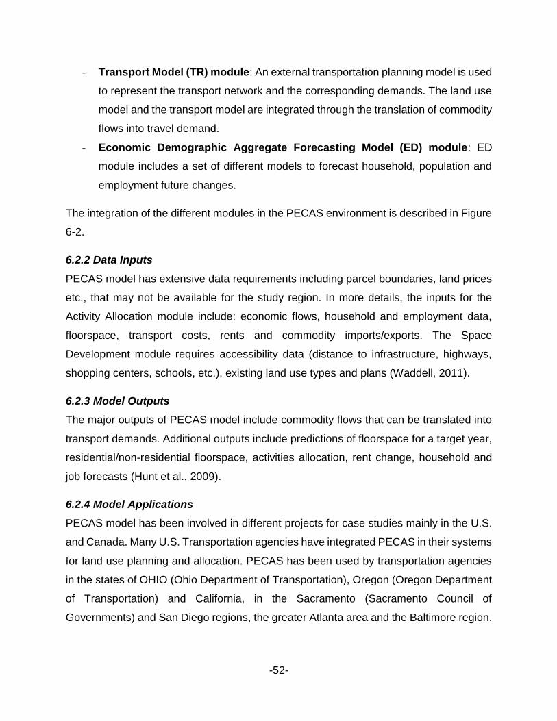
-52-

- Transport Model (TR) module: An external transportation planning model is used

to represent the transport network and the corresponding demands. The land use

model and the transport model are integrated through the translation of commodity

flows into travel demand.

- Economic Demographic Aggregate Forecasting Model (ED) module: ED

module includes a set of different models to forecast household, population and

employment future changes.

The integration of the different modules in the PECAS environment is described in Figure

6-2.

6.2.2 Data Inputs

PECAS model has extensive data requirements including parcel boundaries, land prices

etc., that may not be available for the study region. In more details, the inputs for the

Activity Allocation module include: economic flows, household and employment data,

floorspace, transport costs, rents and commodity imports/exports. The Space

Development module requires accessibility data (distance to infrastructure, highways,

shopping centers, schools, etc.), existing land use types and plans (Waddell, 2011).

6.2.3 Model Outputs

The major outputs of PECAS model include commodity flows that can be translated into

transport demands. Additional outputs include predictions of floorspace for a target year,

residential/non-residential floorspace, activities allocation, rent change, household and

job forecasts (Hunt et al., 2009).

6.2.4 Model Applications

PECAS model has been involved in different projects for case studies mainly in the U.S.

and Canada. Many U.S. Transportation agencies have integrated PECAS in their systems

for land use planning and allocation. PECAS has been used by transportation agencies

in the states of OHIO (Ohio Department of Transportation), Oregon (Oregon Department

of Transportation) and California, in the Sacramento (Sacramento Council of

Governments) and San Diego regions, the greater Atlanta area and the Baltimore region.

-53-

The model has also been applied at the greater areas of Calgary and Edmonton in

Canada (Waddell, 2011).

Figure 6-2: PECAS Structure (Adapted from: Hunt et al. 2009)

6.3 Recommendation for improved land use planning for residential and workplace

location choices

The literature shows that land use models use unsegmented residential and work place

location choice models. Though there are number of latent choices present that

unsegmented models are not able to capture the effect, segmented models can

potentially improve the accuracy of residential and workplace location choices. Future

research is needed to compare the performance of unsegmented and segmented land

use models in predicting land use model outcomes.

-54-

CHAPTER 7: CONCLUSION

Simple discrete choice models use deterministic rules regarding the availability of

alternatives whereas latent choice models provide significant behavioral improvements

by adequately incorporating traits of the market segments. The Manski model that

assumes a two-stage representation of decision making served as the mainstay model

for latent choice set modeling. However, estimation of the Manski model is not always

feasible because calculation of the resulting likelihood function requires enumeration of

all possible choice sets and weighted average of alternative probabilities over these

choice set probabilities. In this context, researchers tried to develop implicit choice set

models that directly tweak the utility functions of alternatives that are considered

probabilistically to approximate the likelihood function in the Manski model. The

advantage of these implicit choice set models is that evaluation of the likelihood function

in these models has linear complexity with respect to the number of alternatives in the

universal choice set.

The proposed model offers significant behavioral advantages by identifying market

segments with differential sensitivities to various attributes and characteristics for

household and workplace location choices to assist targeted policy programs can be

designed by planning agencies. From a forecasting standpoint, latent class models can

substantially improve the model fit and serve as a significant and necessary step towards

developing adequate residential and workplace choices to be further used for land use

and transportation planning. Latent class segmentation can help provide crucial insights

into spatial characteristics, geographic boundaries, multimodal accessibilities, land-use

preferences along with socioeconomic attributes to understand location choices and

travel behavior for medium and long term planning.

Latent choice modeling has served as a valuable modeling method for identifying

population segments with significant behavioral heterogeneity, probabilistic choice sets,

decision rule heterogeneity, and alternate dependency pathways among inter-dependent

choices. However, studies that used latent choice methods in the context of location

choices are relatively rare. This is primarily because of large choice sets in zonal-level

destination choice models that make it unwieldy for estimating latent class models. This

-55-

paper developed a latent class model that explicitly accounts for probabilistic nature of

choice sets by using a two-stage modeling framework that assumes people first pick a

neighborhood and then look for specific locations within the chosen neighborhood. The

expected utility from the second stage zonal choice model component was used as an

explanatory variable in the utility specification of neighborhood choice model to link the

two models. The model was used to analyze residential and work location decisions in

Nashville, Tennessee. The model results indicate significant heterogeneity in the

consideration probability of different neighborhood alternatives both in the residential and

work location choices. Also, the latent class neighborhood models were found to

outperform standard MNL models that assume all decision makers consider the complete

universal choice set in their decision making. The model applicability was demonstrated

by calculating elasticity effects and identifying demographic groups with considerably

different residential and work location preferences.

-56-

APPENDIX A: OVERVIEW OF CASE STUDY DATA

Figure A-1. Distribution of schools in Nashville MPO area

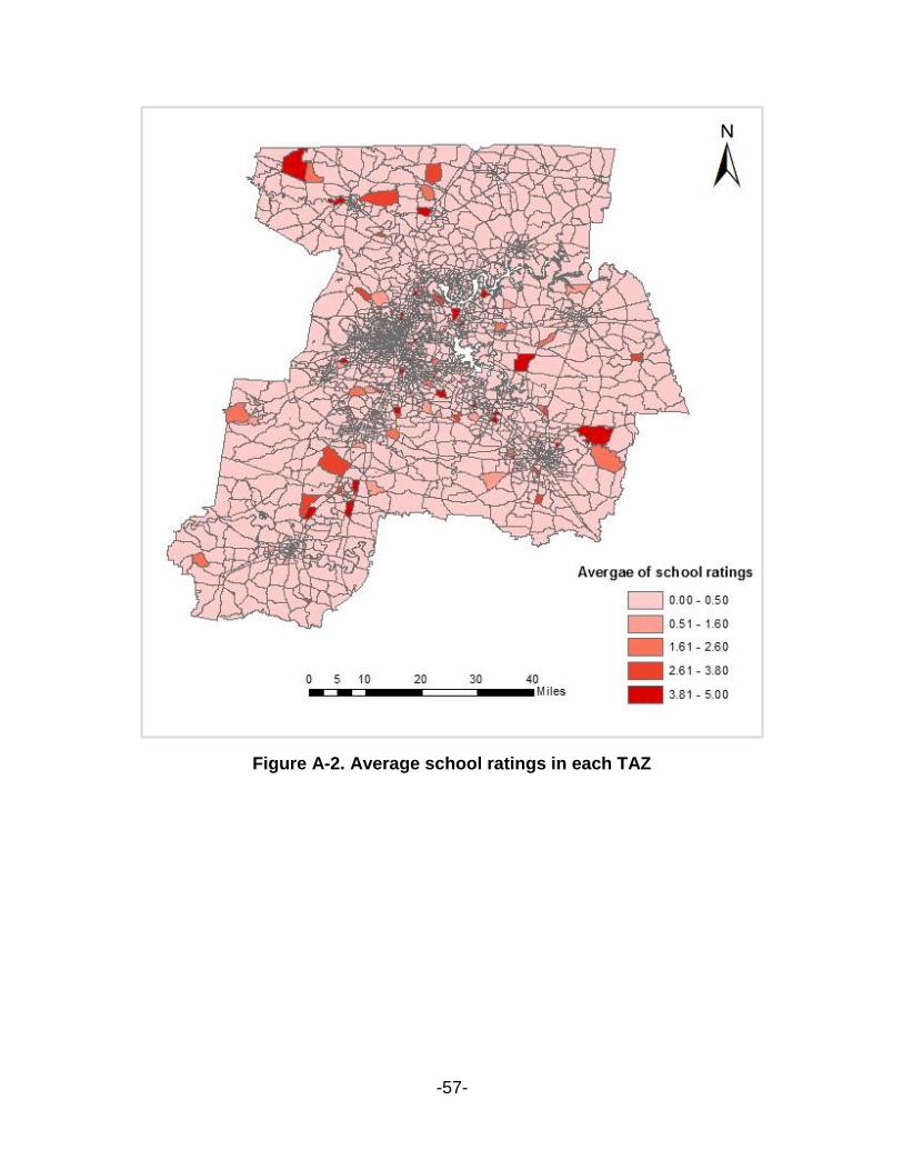
-57-

Figure A-2. Average school ratings in each TAZ

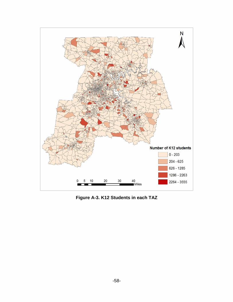
-58-

Figure A-3. K12 Students in each TAZ

-59-

Figure A-4. Population: Age<17 years

-60-

Figure A-5. High and Low-income category households

-61-

REFERENCES

Arunotayanun, K., Polak, J.W., 2011. Taste heterogeneity and market segmentation in

freight shippers’ mode choice behaviour. Transportation Research Part E:

Logistics and Transportation Review 47, 138–148. doi:10.1016/j.tre.2010.09.003

Baerenklau, K.A., 2010. A Latent Class Approach to Modeling Endogenous Spatial

Sorting in Zonal Recreation Demand Models. Land Economics 86, 800–816.

doi:10.3368/le.86.4.800

Bandeen-Roche, K., Xue, Q.-L., Ferrucci, L., Walston, J., Guralnik, J.M., Chaves, P.,

Zeger, S.L., Fried, L.P., 2006. Phenotype of Frailty: Characterization in the

Women’s Health and Aging Studies. J Gerontol A Biol Sci Med Sci 61, 262–266.

Ben-Akiva, M., Boccara, B., 1995. Consideration setsDiscrete choice models with latent

choice sets. International Journal of Research in Marketing 12, 9–24.

doi:10.1016/0167-8116(95)00002-J

Ben-Akiva, M.E., Lerman, S.R., 1985. Discrete choice analysis: theory and application to

travel demand. MIT press.

Bhat, C.R., 1998. Accommodating variations in responsiveness to level-of-service

measures in travel mode choice modeling. Transportation Research Part A: Policy

and Practice 32, 495–507.

Bhat, C.R., 1997. An Endogenous Segmentation Mode Choice Model with an Application

to Intercity Travel. Transportation Science 31, 34–48. doi:10.1287/trsc.31.1.34

Bhat, C.R., Guo, J.Y., 2007. A comprehensive analysis of built environment

characteristics on household residential choice and auto ownership levels.

Transportation Research Part B: Methodological 41, 506–526.

doi:10.1016/j.trb.2005.12.005

Bierlaire, M., Hurtubia, R., Flötteröd, G., 2009. A comparative analysis of implicit and

explicit methods to model choice set generation. Presented at the 9th Swiss

Transport Research Conference.

Boxall, P.C., Adamowicz, W.L., 2002. Understanding heterogeneous preferences in

random utility models: a latent class approach. Environmental and resource

economics 23, 421–446.

-62-

Boxall, P.C., Adamowicz, W.L., Boxall, P.C., n.d. Understanding Heterogeneous

Preferences in Random Utility Models: A Latent Class Approach. Environmental

and Resource Economics 23, 421–446. doi:10.1023/A:1021351721619

Bucholz, K.K., Heath, A.C., Reich, T., Hesselbrock, V.M., Krarner, J.R., Nurnberger, J.I.,

Schuckit, M.A., 1996. Can We Subtype Alcoholism? A Latent Class Analysis of

Data from Relatives of Alcoholics in a Multicenter Family Study of Alcoholism.

Alcoholism: Clinical and Experimental Research 20, 1462–1471.

doi:10.1111/j.1530-0277.1996.tb01150.x

Campbell, D., Lorimer, V., Aravena, C., Hutchinson, G., 2010. Attribute processing in

environmental choice analysis: implications for willingness to pay. Agricultural

Economics 29, 31.

Cascetta, E., Papola, A., 2001. Random utility models with implicit availability/perception

of choice alternatives for the simulation of travel demand. Transportation Research

Part C: Emerging Technologies 9, 249–263. doi:10.1016/S0968-090X(00)00036-

X

Chakraborty, A., Mishra, S., Kim, Y., 2012. Planning support systems and planning across

scales: Comparing scenarios using multiple regional delineations and projections.

Journal of the Urban and Regional Information Systems Association 24, 53–62.

Dillon, W.R., Böckenholt, U., De Borrero, M.S., Bozdogan, H., De Sarbo, W., Gupta, S.,

Kamakura, W., Kumar, A., Ramaswamy, B., Zenor, M., 1994. Issues in the

Estimation and Application of Latent Structure Models of Choice. Marketing Letters

5, 323–334.

Greene, W.H., Hensher, D.A., 2003. A latent class model for discrete choice analysis:

contrasts with mixed logit. Transportation Research Part B: Methodological 37,

681–698.

Grover, R., Srinivasan, V., 1987. A Simultaneous Approach to Market Segmentation and

Market Structuring. Journal of Marketing Research 24, 139–153.

doi:10.2307/3151504

Hensher, D.A., 2010. Attribute processing, heuristics and preference construction in

choice analysis. State-of Art and State-of Practice in Choice Modelling, Emerald

Press, UK 35–70.

-63-

Hensher, D.A., Greene, W.H., 2009. Non-attendance and dual processing of common-

metric attributes in choice analysis: a latent class specification. Empir Econ 39,

413–426. doi:10.1007/s00181-009-0310-x

Hensher, D.A., Rose, J.M., Greene, W.H., 2011. Inferring attribute non-attendance from

stated choice data: implications for willingness to pay estimates and a warning for

stated choice experiment design. Transportation 39, 235–245.

doi:10.1007/s11116-011-9347-8

Hess, S., Rose, J.M., 2007. A latent class approach to recognising respondents’

information processing strategies in SP studies.

Hess, S., Stathopoulos, A., 2013. A mixed random utility — Random regret model linking

the choice of decision rule to latent character traits. Journal of Choice Modelling,

Issues in Choice Modelling: selected papers from the 13th International

Conference on Travel Behaviour Research 9, 27–38.

doi:10.1016/j.jocm.2013.12.005

Hess, S., Stathopoulos, A., Campbell, D., O’Neill, V., Caussade, S., O’Neill, V., Campbell,

D., Hess, S., Stathopoulos, A., 2012. It’s not that I don’t care, I just don’t care very

much: confounding between attribute non-attendance and taste heterogeneity.

Transportation 40, 583–607. doi:10.1007/s11116-012-9438-1

Hunt, J.D., Abraham, J.E., 2009. PECAS—for Spatial Economic Modeling. Calgary,

Alberta: HBA Specto Incorporated.

Hunt, J.D., Abraham, J.E., Silva, D.D., 2009. PECAS-for Spatial Economic Modeling.

SCAG modeling status and next steps. System Documentation Technical Note.

Calgary, Alberta - Google Search [WWW Document]. URL (accessed 12.1.16).

Hynes, S., Hanley, N., Scarpa, R., 2008. Effects on Welfare Measures of Alternative

Means of Accounting for Preference Heterogeneity in Recreational Demand

Models. Am. J. Agr. Econ. 90, 1011–1027. doi:10.1111/j.1467-8276.2008.01148.x

Iacono, M., Levinson, D., El-Geneidy, A., 2008. Models of transportation and land use

change: a guide to the territory. Journal of Planning Literature 22, 323–340.

Jung, T., Wickrama, K. a. S., 2008. An Introduction to Latent Class Growth Analysis and

Growth Mixture Modeling. Social and Personality Psychology Compass 2, 302–

317. doi:10.1111/j.1751-9004.2007.00054.x

-64-

Lanza, S.T., Rhoades, B.L., 2011. Latent Class Analysis: An Alternative Perspective on

Subgroup Analysis in Prevention and Treatment. Prev Sci 14, 157–168.

doi:10.1007/s11121-011-0201-1

Manski, C.F., 1977. The structure of random utility models. Theor Decis 8, 229–254.

doi:10.1007/BF00133443

Martínez, F., Aguila, F., Hurtubia, R., 2009. The constrained multinomial logit: A semi-

compensatory choice model. Transportation Research Part B: Methodological 43,

365–377. doi:10.1016/j.trb.2008.06.006

McFadden, D., 1978. Modeling The Choice of Residential Location. Transportation

Research Record.

Mishra, S., Ye, X., Ducca, F., Knaap, G.-J., 2011. A functional integrated land use-

transportation model for analyzing transportation impacts in the Maryland-

Washington, DC Region. Sustainability: Science, Practice, & Policy 7, 60–69.

Mitani, Y., Shoji, Y., Kuriyama, K., 2008. Estimating economic values of vegetation

restoration with choice experiments: a case study of an endangered species in

Lake Kasumigaura, Japan. Landscape Ecol Eng 4, 103–113. doi:10.1007/s11355-

008-0049-0

Paleti, R., 2015. Implicit choice set generation in discrete choice models: Application to

household auto ownership decisions. Transportation Research Part B:

Methodological 80, 132–149. doi:10.1016/j.trb.2015.06.015

Russell, G.J., Kamakura, W.A., 1993. Measuring brand value with scanner data.

International journal of research in marketing 10, 9–22.

Scarpa, R., Thiene, M., 2005. Destination Choice Models for Rock Climbing in the

Northeastern Alps: A Latent-Class Approach Based on Intensity of Preferences.

Land Economics 81, 426–444. doi:10.3368/le.81.3.426

Sivakumar, A., 2007. Modelling transport: a synthesis of transport modelling

methodologies. Imperial College of London.

Srinivasan, K., Naidu, G., Sutrala, T., 2009. Heterogeneous Decision Rule Model of Mode

Choice Incorporating Utility Maximization and Disutility Minimization.

Transportation Research Record: Journal of the Transportation Research Board

2132, 59–68. doi:10.3141/2132-07

-65-

Swait, J., 1994. A structural equation model of latent segmentation and product choice

for cross-sectional revealed preference choice data. Journal of Retailing and

Consumer Services 1, 77–89. doi:10.1016/0969-6989(94)90002-7

Swait, J., Ben-Akiva, M., 1987. Incorporating random constraints in discrete models of

choice set generation. Transportation Research Part B: Methodological 21, 91–

102. doi:10.1016/0191-2615(87)90009-9

Swait, J., Sweeney, J.C., 2000. Perceived value and its impact on choice behavior in a

retail setting. Journal of Retailing and Consumer Services 7, 77–88.

Waddell, P., 2011. Spatial Input-Output Models: PECAS. Webinar 4 of an 8-part TMIP

Webinar series on land use forecasting methods.

Waddell, P., 2002. UrbanSim: Modeling urban development for land use, transportation,

and environmental planning. Journal of the American Planning Association 68,

297–314.

Waddell, P., 2000. A behavioral simulation model for metropolitan policy analysis and

planning: residential location and housing market components of UrbanSim.

Environment and planning B: Planning and Design 27, 247–263.

Waddell, P., Bhat, C., Eluru, N., Wang, L., Pendyala, R., 2007. Modeling interdependence

in household residence and workplace choices. Transportation Research Record:

Journal of the Transportation Research Board.

Waddell, P., Wang, L., Liu, X., 2008. UrbanSim: an evolving planning support system for

evolving communities. Planning support systems for cities and regions 103–138.

Walker, J.L., Li, J., 2006. Latent lifestyle preferences and household location decisions.

J Geograph Syst 9, 77–101. doi:10.1007/s10109-006-0030-0

Wen, C.-H., Lai, S.-C., 2010. Latent class models of international air carrier choice.

Transportation Research Part E: Logistics and Transportation Review, Selected

Papers from the 12th ATRS Conference 46, 211–221.

doi:10.1016/j.tre.2009.08.004

Wen, C.-H., Wang, W.-C., Fu, C., 2012. Latent class nested logit model for analyzing

high-speed rail access mode choice. Transportation Research Part E: Logistics

and Transportation Review 48, 545–554.

-66-

White, W., 2010. FSUTMS/Land Use Model Integration. Presented to the Florida Model

Task Force.

Zhang, J., Kuwano, M., Lee, B., Fujiwara, A., 2009. Modeling household discrete choice

behavior incorporating heterogeneous group decision-making mechanisms.

Transportation Research Part B: Methodological, Modeling Household Activity

Travel Behavior 43, 230–250. doi:10.1016/j.trb.2008.05.002

LATENT CLASS ANALYSIS OF RESIDENTIAL AND WORK …€¦ · LATENT CLASS ANALYSIS OF RESIDENTIAL AND...

Documents

Transcript of LATENT CLASS ANALYSIS OF RESIDENTIAL AND WORK …€¦ · LATENT CLASS ANALYSIS OF RESIDENTIAL AND...