LLászló Márkus and Péter Elekászló Márkus and Péter Elek

Dept. Probability Theory and StatisticsDept. Probability Theory and Statistics

Eötvös Loránd UniversityEötvös Loránd University

Budapest, HungaryBudapest, Hungary

River Tisza and its aquiferRiver Tisza and its aquifer

Water discharge at VásárosnaményWater discharge at Vásárosnamény(We have 5 more monitoring sites)(We have 5 more monitoring sites)

from1901-2000from1901-2000

Empirical and smoothed seasonal Empirical and smoothed seasonal componentscomponents

Autocorrelation functionAutocorrelation function is slowly is slowly decayingdecaying

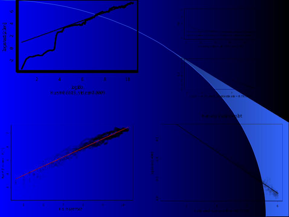
Indicators of long memoryIndicators of long memory

Nonparametric statistics– Rescaled adjusted range or R/S

• Classical

• Lo’s (test)

• Taqqu’s graphical (robust)

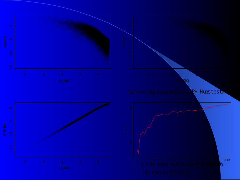
– Variance plot– Log-periodogram (Geweke-Porter Hudak)

2 4 6 8 10

logido,

-20

24

6

logr

star

1[2:

len]

Hurst=0.6603, std.err=0.0009

0 20 40 60 80

Crossing upper critical bound at 44

02

46

8

Vq

N

0 1 2 3 4

Slope = -0.2913945, Hurst estimate = 0.7913945

0.4

0.6

0.8

1.0

1.2

1.4

1.6

1.8

lVq

N

5 6 7 8 9 10

R/S: 0.6807567

34

56

7

Rp

erS

[1:(

sza

mo

l - 2

), 1

]

3 4 5 6

-2.0

-1.5

-1.0

-0.5

log

(szo

ras[

1:4

00

])

Nameny Variance plot

Estimated Hurst coefficient=0.73782

-8 -6 -4 -2 0

logfreq

-15

-10

-50

logs

pec

-15 -10 -5 0

GPHfreq

-15

-10

-50

logs

pec

-8 -6 -4 -2 0

logfreq

-15

-10

-50

GP

Hfre

q

0 500 1000 1500 2000 2500

fi

0.5

0.6

0.7

0.8

0.9

hu

rstc

fs

Nameny log-periodogram, GPH-Hurst estimation

Estimated Hurst coeff= 0.84796, (mean of [22:55])

Linear long-memory model : Linear long-memory model : fractional fractional ARIMA-processARIMA-process

(Montanari et al., (Montanari et al., Lago Maggiore, Lago Maggiore, 1997)1997) Fractional ARIMA-model:

Fitting is done by Whittle-estimator:– based on the empirical and theoretical periodogram– quite robust: consistent and asymptotically normal

for linear processes driven by innovatons with finite forth moments (Giraitis and Surgailis, 1990)

ttd BXBB )()1()(

Results of Results of fractional fractional ARIMAARIMA fitfit

H=0.846 (standard error: 0.014) p-value: 0.558 (indicates goodness of fit) Innovations can be reconstructed using a linear filter

(the inverse of the filter above)

tt BXBBB )21.01()1()12.080.01( 34.02

Reconstruct the innovation from the Reconstruct the innovation from the fitted modelfitted model

Reconstructed innovations are uncorrelatedReconstructed innovations are uncorrelated......

But not independentBut not independent

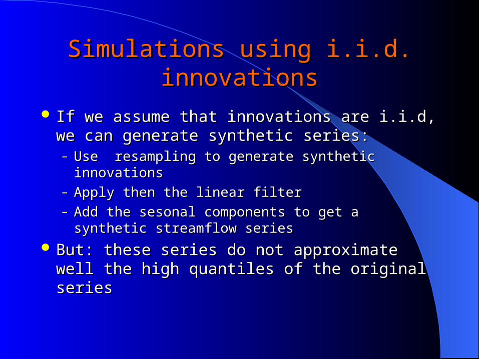
Simulations using i.i.d. innovationsSimulations using i.i.d. innovations

If we assume that innovations are i.i.d, we can If we assume that innovations are i.i.d, we can generate synthetic series:generate synthetic series:– Use resampling to generate synthetic innovations Use resampling to generate synthetic innovations – Apply then the linear filter Apply then the linear filter – Add the sesonal components to get a synthetic Add the sesonal components to get a synthetic

streamflow series streamflow series

But: these series do not approximateBut: these series do not approximate well well the high the high quantiles of the original seriesquantiles of the original series

But: they fail to catch the densities and But: they fail to catch the densities and underestimate the high quantiles of the underestimate the high quantiles of the

original seriesoriginal series

Innovations can be regarded as shocks to the linear system

Few properties:– Squared and absolute values are autocorrelated– Skewed and peaked marginal distribution– There are periods of high and low variance

All these point to a GARCH-type modelThe classical GARCH is far too heavy

tailed to our purposes

SimulationSimulation from the GARCH-process from the GARCH-process

Simulations:– Generate i.i.d. series from

the estimated GARCH-residuals

– Then simulate the GARCH(1,1) process using these residuals

– Apply the linear filter and the seasonalities

The simulated series are much heavier-tailed than the original series

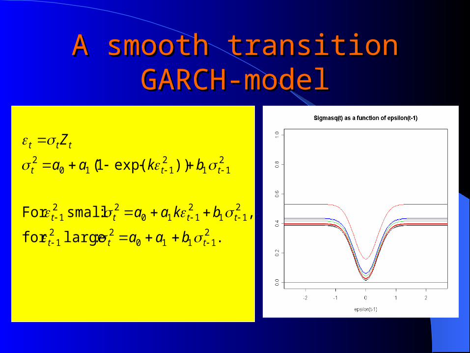
A smooth transition GARCH-A smooth transition GARCH-modelmodel

. :large for

, :small For

))exp(1(

21110

221

211

2110

221

211

2110

2

ttt

tttt

ttt

ttt

baa

bkaa

bkaa

Z

ACF of GARCH-residualsACF of GARCH-residuals

Results of simulationsResults of simulationsat Vat Váássáárosnamrosnaményény

Back to the original GARCH philosophyBack to the original GARCH philosophy

The above described GARCH model is somewhat artificial, and hard to find heuristic explanations for it:– why does the conditional variance depend on the

innovations of the linear filter?– in the original GARCH-context the variance is

dependent on the lagged values of the process itself. Possible solution: condition the variance on the lagged

discharge process instead ! Theoretical problems (e.g. on stationarity) arise but

heuristically clear explanation can be given more easily

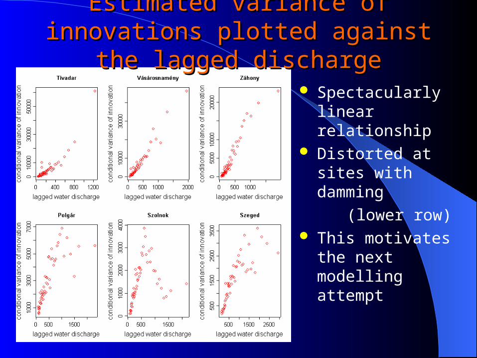
Estimated variance of innovationEstimated variance of innovationss plotted against the lagged dischargeplotted against the lagged discharge

Spectacularly linear relationship

Distorted at sites with damming

(lower row) This motivates the next

modelling attempt

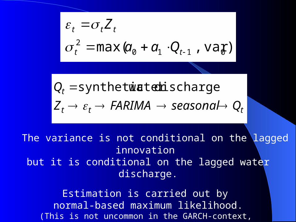
  The variance is not conditional on the lagged innovation but it is conditional on the lagged water discharge.

Estimation is carried out by normal-based maximum likelihood.

(This is not uncommon in the GARCH-context, even if the residuals are non-Gaussian. See McNeil and Frey, 2000)

)var , max( 01102

tt

ttt

Qaa

Z

ttt

t

QseasonalFARIMAZ

Q

discharge water synthetic

How to simulate the residuals of How to simulate the residuals of the new GARCH-the new GARCH-typetype modelmodel

Residuals are highly skewed and peaked.

Simulation:– Use resampling to simulate

from the central quantiles of the distribution

– Use Generalized Pareto distribution to simulate from upper and lower quantiles

– Use periodic monthly densities

The simulation processThe simulation process

t

Zt

Xt

resampling and GPD

FARIMA filter

GARCH-type model

Seasonal filter

Evaluating the modelEvaluating the model fit fit

Independence of residual series ACF, extremal clustering

Fit of probability density and high quantilesVariance – lagged discharge relationshipExtremal indexConsistence of parameter estimates

ACF of original and squared ACF of original and squared innovation series – residual seriesinnovation series – residual series

Results of Results of new new simulationssimulationsat Vat Váássáárosnamrosnaményény

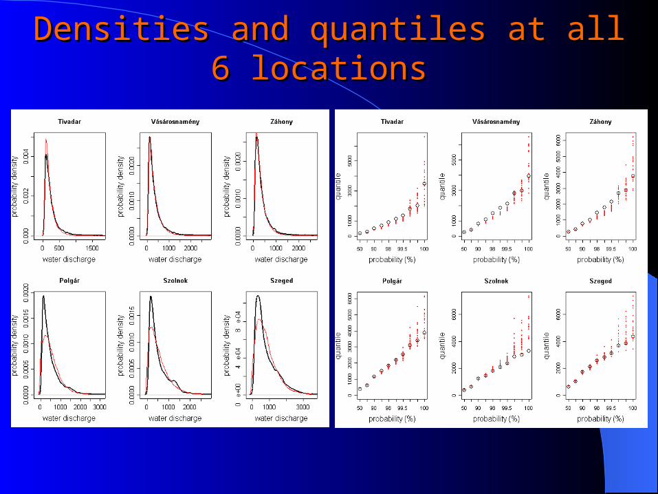
Densities and quantiles at all 6 locations Densities and quantiles at all 6 locations

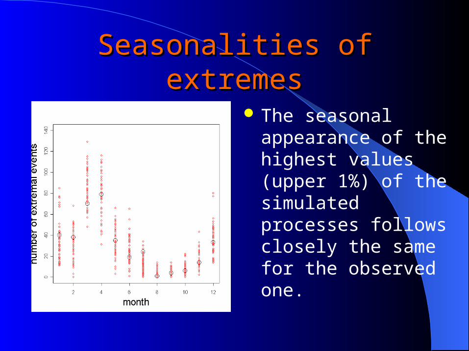
Seasonalities of extremesSeasonalities of extremes

The seasonal appearance of the highest values (upper 1%) of the simulated processes follows closely the same for the observed one.

Estimated extremal indices displayedEstimated extremal indices displayed

Multivariate modellingMultivariate modelling Final aim: to model the runoff processes simultaneously Nonlinear interdependence and non-Gaussianity should

be addressed here, too First, the joint behaviour of the discharges inflowing

into Hungary should be modelled Differential equation-oriented models of conventional

hydrology may be used to describe downstream evolution of runoffs

Now we concentrate on joint modelling of two rivers: Tisza (at Tivadar) and Szamos (at Csenger)

Issues of joint modellingIssues of joint modelling

Measures of linear interdependences (the cross-correlations) are likely to be insufficient.

High runoffs appear to be more synchronized on the two rivers than small ones

The reason may be the common generating weather patterns for high flows

This requires a non-conventional analysis of the dependence structure of the observed series

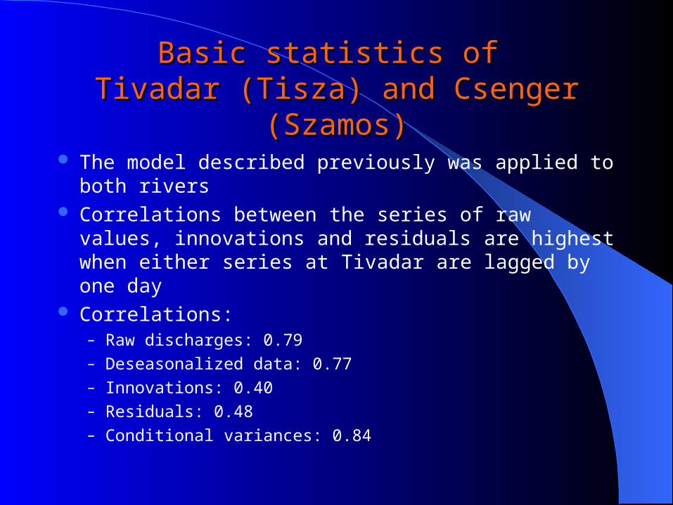
Basic statistics of Basic statistics of Tivadar (Tisza) and Csenger (Szamos)Tivadar (Tisza) and Csenger (Szamos)

The model described previously was applied to both rivers Correlations between the series of raw values, innovations

and residuals are highest when either series at Tivadar are lagged by one day

Correlations:– Raw discharges: 0.79– Deseasonalized data: 0.77– Innovations: 0.40 – Residuals: 0.48– Conditional variances: 0.84

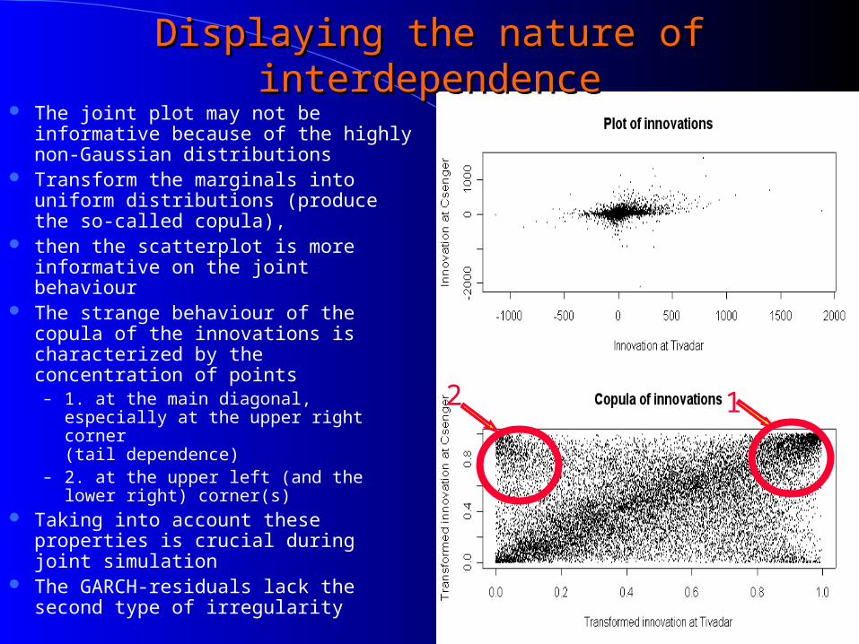
Displaying the nature of interdependenceDisplaying the nature of interdependence The joint plot may not be informative

because of the highly non-Gaussian distributions

Transform the marginals into uniform distributions (produce the so-called copula),

then the scatterplot is more informative on the joint behaviour

The strange behaviour of the copula of the innovations is characterized by the concentration of points

– 1. at the main diagonal, especially at the upper right corner (tail dependence)

– 2. at the upper left (and the lower right) corner(s)

Taking into account these properties is crucial during joint simulation

The GARCH-residuals lack the second type of irregularity

12

A possible explanation of this type of interdependenceA possible explanation of this type of interdependence The cond. variance process is

essentially common for the two rivers (correlation = 0.84)

This gives a hint to explain the interdependence of the innovations:

– Generate two interdependent residual series (correlation=0.48)

– Multiply by a common standard deviation process (distributed as Gamma)

– The obtained copula is very similar to the observed copula of the innovations

This justifies the hypothesis that the common variance causes the interdependence of the given type

Thank you for your attentionThank you for your attention!!