Last Time Main memory indexing (T trees) and a real system. Optimize for CPU, space, and logging.
24
• Last Time – Main memory indexing (T trees) and a real system. – Optimize for CPU, space, and logging. • But things have changed drastically! • Hardware trend: – CPU speed and memory capacity double every 18 months. – Memory performance merely grows 10%/yr •Capacity v.s. Speed (esp. latency) – The gap grows ten fold every 6 yr! And 100 times since 1986.
-
Upload
driscoll-duke -
Category
Documents
-
view
29 -
download
0
description
Last Time Main memory indexing (T trees) and a real system. Optimize for CPU, space, and logging. But things have changed drastically! Hardware trend: CPU speed and memory capacity double every 18 months. Memory performance merely grows 10%/yr Capacity v.s. Speed (esp. latency) - PowerPoint PPT Presentation
Transcript of Last Time Main memory indexing (T trees) and a real system. Optimize for CPU, space, and logging.

• Last Time– Main memory indexing (T trees) and a real system.– Optimize for CPU, space, and logging.
• But things have changed drastically!• Hardware trend:
– CPU speed and memory capacity double every 18 months.
– Memory performance merely grows 10%/yr• Capacity v.s. Speed (esp. latency)
– The gap grows ten fold every 6 yr! And 100 times since 1986.

Implications:– Many databases can fit in main memory.
– But memory access will become the new bottleneck.
– No longer a uniform random access model!
– Cache performance becomes crucial.

• Cache conscious indexing J. Rao and K. A. Ross
– ``Cache Conscious Indexing for Decision-Support in Main Memory'' , VLDB 99.
– ``Making B+-Trees Cache Conscious in Main Memory'' SIGMOD 2000.
• Cache conscious join algorithms. – Peter A. Boncz, Stefan Manegold, Martin L. Kersten:
Database Architecture Optimized for the New Bottleneck: Memory Access. VLDB 1999.

Memory Basics
• Memory hierarchy:– CPU– L1 cache (on-chip): 1 cycle, 8-64 KB, 32 byte/line– L2 cache: 2-10 cycle, 64 KB-x MB, 64-128 byte/line– MM: 40-100 cycle, 128MB-xGB, 8-16KB/page– TLB: 10-100 cycle. 64 entries (64 pages).– Capacity restricted by price/performance.
• Cache performance is crucial– Similar to disk cache (buffer pool)– Catch: DBMS has no direct control.

Improving Cache Behavior• Factors:
– Cache (TLB) capacity.
– Locality (temporal and spatial).
• To improve locality:– Non random access (scan, index traversal):
• Clustering to a cache line.
• Squeeze more operations (useful data) into a cache line.
– Random access (hash join):
• Partition to fit in cache (TLB).
– Often trade CPU for memory access

Cache Conscious Indexing- J. Rao and K. A. Ross
• Search only (without updates)– Cache Sensitive Search Trees.
• With updates– Cache sensitive B+ trees and variants.

Existing Index Structures (1)
• Hashing. – Fastest search for small bucket chain.– Not ordered – no range query.– Far more space than tree structure index.
• Small bucket chain length -> many empty buckets.

Existing Index Structures (2)• Average log 2 N comparisons for all tree structured
index.• Binary search over a sorted array.
– No extra space.– Bad cache behavior. About one miss/comparison.
• T trees.– No better. One miss every 1 or 2 comparisons.
1 2 3 4 5 6 7 10 12 27 88 101 103 105
3 12
d1, d2, d3,d4,d5…dn

Existing Index Structures (3)
• B+ tree – Good: one miss/node if each node fits in a cache line.
– Overall misses: log m n, m as number of keys per node,
n as total number of keys.
• To improve – increase m (fan-out)
– i.e., squeeze more comparisons (keys) in each node.• Half of space used for child pointers.

Cache Sensitive Search Tree• Key: Improve locality• Similar as B+ tree (the best existing).• Fit each node into a L2 cache line
– Higher penalty of L2 misses.– Can fit in more nodes than L1. (32/4 v.s. 64/4)
• Increase fan-out by:– Variable length keys to fixed length via dictionary compression.– Eliminating child pointers
• Storing child nodes in a fixed sized array.• Nodes are numbered & stored level by level, left to right.• Position of child node can be calculated via arithmetic.

1 2 3 4 1 2 3 4
1 3
2
B+ tree, 2-way, 3 misses
21 3
Suppose cache line size = 12 bytes,
Key Size = Pointer Size = 4 bytes
CSS tree, 4-way, 2 misses
Node0
Node1 Node2 Node3 Node4
Search K = 3,
Match 3rd key in Node 0.
Node# =
0*4 + 3 = Node 3

Performance Analysis (1)• Node size = cache line size is optimal:
– Node size as S cache lines.– Misses within a node = 1 + log 2 S
• Miss occurs when the binary search distance >= 1 cache line
– Total misses = log m n * ( 1 + log 2 S )– m = S * c (c as #of keys per cache line, constant)– Total misses = A / B where:
• A = log2 n * (1+log2 S)• B = log2 S + log2 c
– As log2S increases by one, A increases by log2 n, B by 1. – So minimal as log2S = 0, S = 1

Performance Analysis (2)• Search improvement over B+ tree:
– log m/2 n / log m n – 1 = 1/(log2 m –1)– As cache line size = 64 B, key size = 4, m = 16, 33%.– Why this technique not applicable for disks?
• Space– About half of B+ tree (pointer saved)– More space efficient than hashing and T trees.– Probably not as high as paper claimed since RID not counted.
• CSS has the best search/space balance.– Second the best search time (except Hash – very poor space)– Second the best space (except binary search – very poor search)

Problem?
• No dynamic update because fan-out and array size must be fixed.

With Update- Restore Some Pointers
• CSB+ tree– Children of the same node stored in an array (node group)
– Parent node with only a pointer to the child array.
– Similar search performance as CSS tree. (m decreases by 2)
– Good update performance if no split.

Other Variants• CSB+ tree with segments
– Divide child array into segments (usually 2)– With one child pointer per segment– Better split performance, but worse search.
• Full CSB+ tree – CSB+ tree with pre-allocated children array.– Good for both search and insertion. But more space.
2-segment CSB+ tree.
Fan-out drops by 2*2.

Performance
• Performance:– Search: CSS < full CSB+ ~ CSB+ < CSB+ seg < B+
– Insertion: B+ ~ full CSB+ < CSB+ seg < CSB+ < CSS
• Conclusion:– Full CSB+ wins if space not a concern.
– CSB+ and CSB+ seg win if more reads than insertions.
– CSS best for read-only environment.

Cache Conscious Join Method Paper
– Peter A. Boncz, Stefan Manegold, Martin L. Kersten: Database Architecture Optimized for the New Bottleneck: Memory Access. VLDB 1999.
Contributions:– For sequential access:
• Vertical decomposed tables.
– For random access: (hash joins)• Radix algorithm – Fit data in cache and TLB.

An Experiment
• Figure 3, page 56
• Sequential scan with accessing one byte from each tuple.
• Jump of time as tuple length exceeds L1 and L2 cache line size (16-32 bytes, 64-128 bytes)
• For efficient scan, reduce tuple length!
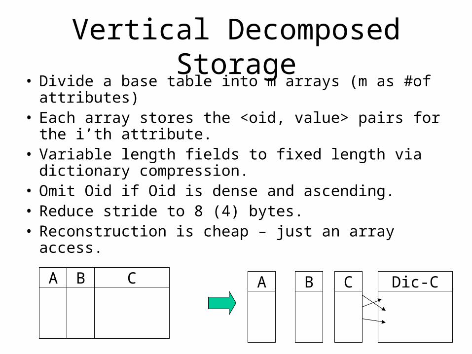
Vertical Decomposed Storage• Divide a base table into m arrays (m as #of attributes)• Each array stores the <oid, value> pairs for the i’th
attribute.• Variable length fields to fixed length via dictionary
compression.• Omit Oid if Oid is dense and ascending.• Reduce stride to 8 (4) bytes. • Reconstruction is cheap – just an array access.
A B C A B Dic-CC

Existing Equal-Join Methods
• Sort-merge: – Bad since usually one of the relation will not fit in cache.
• Hash Join: – Bad if inner relation can not fit in cache.
• Clustered hash join: – One pass to generate cache sized partitions.
– Bad if #of partitions exceeds #cache lines or TLB entries.
.
Cache (TLB) thrashing occurs – one miss per tuple

Radix Join (1)• Multi passes of partition.
– The fan-out of each pass does not exceed #of cache lines AND TLB entries.
– Partition based on B bits of the join attribute (low computational cost)
56781234
0110110001101100
5814
01000100
6723
10111011
84
0000
51
0101
…

Radix Join (2)
• Join matching partitions– Nested-loop for small partitions (<= 8 tuples) – Hash join for larger partitions
• <= L1 cache, L2 cache or TLB size.• Best performance for L1 cache size (smallest).
• Cache and TLB thrashing avoided.• Beat conventional join methods
– Saving on cache misses > extra partition cost

Lessons• Cache performance important, and becoming more
important• Improve locality
– Clustering data into a cache line– Leave out irrelevant data (pointer elimination, vertical
decomposition)– Partition to avoid cache and TLB thrashing
• Must make code efficient to observe improvement– Only the cost of what we consider will improve.– Be careful to: functional calls, arithmetic, memory
allocation, memory copy.