Laser Scanning for Forest Structure Analysis
78
University of Southern Queensland Faculty of Engineering and Surveying Laser Scanning for Forest Structure Analysis A dissertation submitted by Adam John Coburn In fulfilment of the requirements of Courses ENG4111 and ENG4112 Research Project Towards the degree of Bachelor of Spatial Science (Honours), Surveying
Transcript of Laser Scanning for Forest Structure Analysis

University of Southern Queensland Faculty of Engineering and
Surveying
Laser Scanning for
Forest Structure Analysis
A dissertation submitted by
Adam John Coburn
In fulfilment of the requirements of
Courses ENG4111 and ENG4112 Research
Project
Towards the degree of
Bachelor of Spatial Science (Honours),
Surveying

Laser Scanning for Forest Structure Analysis Page 2
Adam Coburn 0061021174
Abstract
Terrestrial laser scanning is one of the most recent technological
advancements within the spatial science industry. Its current use within the
forest analysis field is limited.
Collecting data to create a forest inventory can be a long and strenuous
process with current procedures relying on outdated and inefficient
techniques. Terrestrial laser scanning is a technique that has the potential to
greatly enhance this data collection process.
In this study, a forested area of 6700m2 in eastern Toowoomba has been
scanned to extract tree height, diameter at breast height, basal area and
volume. The same data has been collected using contemporary techniques
so that terrestrial laser scanning’s suitability can be assessed.
The measured components were compared and discrepancies were
identified. When compared to traditional methods, laser scanning
overestimated height by 0.196m (2.42%). Diameter at breast height, basal
area and volume were all underestimated by 0.061m (13.33%), 0.044m2
(24.35%) and 0.374m3 (22.47%) respectively. The differences in height and
diameter at breast height are acceptable. The differences in excess of 20%,
namely basal area and volume, are unacceptable with further research
required to identify both the cause and the solution.

Laser Scanning for Forest Structure Analysis Page 3
Adam Coburn 0061021174
University of Southern Queensland
Faculty of Health, Engineering and Sciences
ENG4111/ENG4112 Research Project
Limitations of Use
The Council of the University of Southern Queensland, its Faculty of
Health, Engineering & Sciences, and the staff of the University of Southern
Queensland, do not accept any responsibility for the truth, accuracy or
completeness of material contained within or associated with this
dissertation.
Persons using all or any part of this material do so at their own risk, and not
at the risk of the Council of the University of Southern Queensland, its
Faculty of Health, Engineering & Sciences or the staff of the University of
Southern Queensland.
This dissertation reports an educational exercise and has no purpose or
validity beyond this exercise. The sole purpose of the course pair entitled
“Research Project” is to contribute to the overall education within the
student’s chosen degree program. This document, the associated hardware,
software, drawings, and other material set out in the associated appendices
should not be used for any other purpose: if they are so used, it is entirely at
the risk of the user.

Laser Scanning for Forest Structure Analysis Page 4
Adam Coburn 0061021174
University of Southern Queensland
Faculty of Health, Engineering and Sciences
ENG4111/ENG4112 Research Project
Certification of Dissertation
I certify that the ideas, designs and experimental work, results, analyses and
conclusions set out in this dissertation are entirely my own effort, except
where otherwise indicated and acknowledged.
I further certify that the work is original and has not been previously
submitted for assessment in any other course or institution, except where
specifically stated.
A. Coburn
0061021174

Laser Scanning for Forest Structure Analysis Page 5
Adam Coburn 0061021174
Acknowledgements
I would like to acknowledge that this research was carried out under the
supervision of Dr. Xiaoye Liu. Her continued guidance has been
irreplaceable.
I would also like to acknowledge the assistance provided by Dr. Zhenyu
Zhang and Mr. James Derksen during the scanning procedure.

Laser Scanning for Forest Structure Analysis Page 6
Adam Coburn 0061021174
Table of Contents
Abstract .......................................................................................................... 2
Acknowledgements ........................................................................................ 5
Table of Contents ........................................................................................... 6
List of Tables.................................................................................................. 9
List of Figures .............................................................................................. 10
Chapter 1 - Introduction ............................................................................... 12
1.1 Introduction ........................................................................................ 12
1.2 Research Aim ..................................................................................... 13
1.3 Justification ........................................................................................ 13
1.4 Dissertation Overview ........................................................................ 14
Chapter 2 - Literature Review ...................................................................... 16
2.1 Introduction ........................................................................................ 16
2.2 What is Laser Scanning? .................................................................... 16
2.3 Types of Laser Scanners .................................................................... 17
2.4 Current Applications of Laser Scanners ............................................ 22
2.5 Forest Structure Analysis ................................................................... 25
2.6 Laser Scanning of Forest Structures .................................................. 27
2.7 Conclusion ......................................................................................... 30
Chapter 3 - Methodology ............................................................................. 31
Laser Scanning for Forest Structure Analysis Page 7
Adam Coburn 0061021174
3.1 Introduction ........................................................................................ 31
3.2 Study Area .......................................................................................... 31
3.3 Equipment .......................................................................................... 33
3.4 Field Procedures ................................................................................. 33
3.5 Post Processing .................................................................................. 36
3.6 Data Comparison ................................................................................ 39
3.7 Conclusion ......................................................................................... 39
Chapter 4 – Results ...................................................................................... 40
4.1 Introduction ........................................................................................ 40
4.2 Traditional Data ................................................................................. 40
4.3 Scanned Data ...................................................................................... 41
4.4 Variations ........................................................................................... 43
4.4 Conclusion ......................................................................................... 47
Chapter 5 – Discussion ................................................................................ 48
5.1 Introduction ........................................................................................ 48
5.2 Quick View Analysis ......................................................................... 48
5.3 Planar View ........................................................................................ 54
5.4 Average of Quick and Planar Measurements ..................................... 56
5.5 Time Comparison ............................................................................... 58
5.6 Conclusion ......................................................................................... 60
Chapter 6 – Conclusions .............................................................................. 61

Laser Scanning for Forest Structure Analysis Page 8
Adam Coburn 0061021174
6.1 Introduction ........................................................................................ 61
6.2 Research Findings .............................................................................. 61
6.3 Further Research and Recommendations ........................................... 62
6.4 Conclusion ......................................................................................... 63
Appendix ...................................................................................................... 64
Appendix 1 – Project Specification.......................................................... 64
Appendix 2 – How Scanners Measure Distance ...................................... 66
Appendix 3 – FARO Scene Cluster ......................................................... 67
Appendix 4 – FARO Scene Quick View ................................................. 69
Appendix 5 – FARO Scene Planar View ................................................. 71
Appendix 6 – Risk Assessment Documents............................................. 72
References .................................................................................................... 74

Laser Scanning for Forest Structure Analysis Page 9
Adam Coburn 0061021174
List of Tables
Table 1. Data obtained from traditional methods. ....................................... 40
Table 2. Quick view tree measurements...................................................... 41
Table 3. Planar view tree measurements. .................................................... 41
Table 4. Average tree measurements from scanned data. ........................... 42
Table 5. Mean height variances and standard deviations. ........................... 43
Table 6. Mean DBH variances and standard deviations.............................. 44
Table 7. Mean basal area variances and standard deviations. ..................... 45
Table 8. Mean volume variances and standard deviations. ......................... 45
Table 9. Percentage variances between scanned average and traditional. .. 45
Table 10. Volume calculated using planar height and quick DBH ............. 57
Table 11. Volume variances between traditional and scanned data. ........... 58

Laser Scanning for Forest Structure Analysis Page 10
Adam Coburn 0061021174
List of Figures
Figure 1. The Leica Scanstation c10 – a time-of-flight scanner. ................ 18
Figure 2. The Leica HDS 6200 – a phase based scanner ............................ 19
Figure 3. The Reigl VZ-400 – a waveform processing scanner.................. 20
Figure 4. Multiple echo detection ............................................................... 21
Figure 5. Toowoomba’s location within Queensland. ................................ 31
Figure 6. Satellite view od the study area. .................................................. 32
Figure 7. One section of the area being analysed. ....................................... 32
Figure 8. The FARO Focus 3D conducting a scan. .................................... 34
Figure 9. Scan locations within the study area. ........................................... 34
Figure 10. Variances in height between scanned data and traditional. ....... 43
Figure 11. Variances in DBH between scanned data and traditional. ......... 44
Figure 12. Variances in basal area between scanned data and traditional. . 44
Figure 13. Variances in volume between scanned data and traditional. ..... 45
Figure 14. Variation as a percentage between scanned data and traditional.
...................................................................................................................... 46
Figure 15. Vertical height error. .................................................................. 49
Figure 16. Tree #18, the largest quick view variation. ................................ 50
Figure 17. Tree #17, the smallest quick view variation. ............................. 50
Figure 18. Tree #20, the smallest DBH variation. ...................................... 52

Laser Scanning for Forest Structure Analysis Page 11
Adam Coburn 0061021174
Figure 19. Tree #11, the largest DBH variation. ......................................... 52

Laser Scanning for Forest Structure Analysis Page 12
Adam Coburn 0061021174
Chapter 1 - Introduction
1.1 Introduction
In the modern era technology is advancing extremely quickly. These
advancements allow for old techniques and practices to be replaced with
safer, quicker and more efficient ones. One such technology is terrestrial
laser scanning (TLS).
Laser scanning is a process which allows for rapid data collection. Millions
of data points can be measured to high accuracy and precision in minutes.
Data such as this is extremely useful in obtaining a detailed understanding
of the features measured.
Not only does laser scanning offer quick data collection, it is also excellent
at providing a visual representation of the data collected. Such high quantity
point clouds allow anyone observing the point cloud to identify exactly what
the object is. This visual aspect, combined with the high accuracy and
precision data allows for effective and efficient data manipulation.
Forest analysis is extremely important in the modern era. Continuing
environmental concern is of high priority to governments and private
corporations. Structure health, growth rate, decay rate and biomass are a
small number of important forest elements identified during an analysis.
Such data must be recorded at a high detail to ensure the structure can be
analysed correctly. Current techniques involve manual measurements and
extensive effort and resultantly have vast room for improvement. Laser

Laser Scanning for Forest Structure Analysis Page 13
Adam Coburn 0061021174
scanning offers the potential to improve the data capture stage of forest
analyses and also offers detailed analysis tools.
1.2 Research Aim
The aim of this study is to assess laser scanning’s suitability when recording
a forest structure. This will be achieved by executing the following
objectives:
a) Identifying the following components of the structure using laser
scanning and traditional methods:
o Tree height.
o Diameter at breast height.
o Basal area.
o Tree volume.
b) Comparing the acquired data and assess laser scanning’s suitability
1.3 Justification
Completing a forest inventory can be a long and strenuous process,
especially if required to be completed by one person. Detailed information
needs to be recorded on each member of the structure. This involves
measuring, taking photos and analysing the individual structure. The data
then needs to be transferred to a computer, analysed again and recorded.
This needs to be completed for all members of the forest structure being
analysed.
Terrestrial laser scanning has been used to improve this process by making
it more efficient. This is through quick data collection and the ability to

Laser Scanning for Forest Structure Analysis Page 14
Adam Coburn 0061021174
easily manipulate the captured data. Another benefit of the technology is the
high level of both accuracy and precision.
As the process of using terrestrial laser scanning to capture forest data
becomes more common, the techniques used will improve. This research is
no exception and aims to not only analyse the results obtained from the data,
but also the suitability of the process to the application.
1.4 Dissertation Overview
This dissertation features six main chapters. A brief description of these
chapters is given below:
Chapter 1: Introduction – Provides an introduction to the research area.
Research aims of the study are highlighted. Background information
regarding the topic and justification of the research is also discussed.
Chapter 2: Literature Review – Identifies the key components as well as a
summary of the literature review conducted for this research. The three
areas of interest are: laser scanning, forest analysis and laser scanning’s
current applications within forest structures.
Chapter 3: Methodology – The methods used to meet the aims of the study
are identified in this chapter. The study area as well as the techniques used
to both capture and analyse the data are discussed.
Chapter 4: Results – Provides the data obtained using the stated
methodology is presented within this chapter.

Laser Scanning for Forest Structure Analysis Page 15
Adam Coburn 0061021174
Chapter 5: Discussion – The raw data obtained is compared and contrasted
to identify relationships. Resultantly the suitability of laser scanning can be
identified.
Chapter 6: Conclusion – Provides a conclusion to the dissertation as well
as recommendations for future research.

Laser Scanning for Forest Structure Analysis Page 16
Adam Coburn 0061021174
Chapter 2 - Literature Review
2.1 Introduction
A literature review was conducted with regard to five key areas: the
explanation of laser scanning, the types of scanners available and how they
work, the current applications of laser scanning, forest inventorying and
structure analysis as well as the application of laser scanning within the
aforementioned field. Consequently the aim of this chapter is to provide
insight on studies conducted in this professional field by analysing
conducted research and studying previous findings.
2.2 What is Laser Scanning?
A laser scanner is hardware that is used to collect 3D data of a real world
object. This allows the object to be analysed effectively and efficiently
using powerful software.
Laser scanning is considered a new technology within the spatial science
and engineering world despite Electronic Distance Measurement (EDM)
being around since the 1960s. This is because it did not become used in this
professional field until the late 1990s (SurvTech Solutions 2014). The
reason this occurred was because the technology could not be used
effectively until computer storage systems and bandwidth improved
(SurvTech Solutions 2014).
Laser scanners can capture points at rates of up to one million per second
(Leica 2010). Such a high quantity of points requires a large amount of
storage with individual raw data files often exceeding one gigabyte.

Laser Scanning for Forest Structure Analysis Page 17
Adam Coburn 0061021174
Consequently the technology is not as ‘mobile’ as data collected by GPS or
total station. Data captured with these two instruments would take weeks of
work to create the same point cloud that is achieved by laser scanning.
Consequently, total station and GPS point clouds only identify key points.
This results in smaller file sizes which are heavily streamlined when
compared to laser scanner point clouds. The storage required to store
scanned point clouds is evidently one limitation associated with the
technology.
If storage issues are overcome, the models created allow for a very detailed
analysis of the real world. This high level of detail has been the force behind
laser scanning’s growth. The technology has improved with scans taking
less time and outputting large quantities of information with high accuracy
and precision.
2.3 Types of Laser Scanners
There are three principle types of scanners: Time-of-Flight, Phase Based
and Triangulation (Payne 2009). Appendix 2 provides a diagram explaining
how time-of-flight and phase based scanners measure distances. Scanners
that slightly alter these principles also exist. These are known as Waveform
Processing scanners scanners.
2.3.1 Time-of-Flight Scanners
Time-of-flight scanners measure distances by analysing the time taken for a
light pulse to bounce from the target object and return to the scanner (Payne
2009). This time is halved and by using the speed of light a distance can be
calculated (3D Systems 2011). This distance is combined with a vertical and

Laser Scanning for Forest Structure Analysis Page 18
Adam Coburn 0061021174
horizontal bearing to create a 3D point in the same position as the target
object. A time-of-flight scanner is best used when large distances need to be
measured.
Figure 1. The Leica Scanstation c10 – a time-of-flight scanner. (Leica
2010).
California Department of Transportation (2011) stated that the maximum
range is typically 125-1000m. The Leica ScanStation C10 (Figure 1) can
measure distances up to 300m. The drawback of time-of-flight scanners is
their slower data acquisition. The Leica ScanStation C10 can capture 50,000
points per second (Leica 2010) and is a relatively fast time-of-flight
instrument.
The accuracy of time-of-flight scanners is determined by the system’s
ability to accurately measure the time of the returning signal (Payne 2009).
Payne (2009) also states that although the accuracy varies across different
systems, typical accuracy for a time-of-flight scanner is 4-10mm over 300m.
Current time-of-flight scanners possess on-board cameras. Photos are taken
before or after the scan within the parameters defined by the user. These
photos are then overlayed on the point cloud to create an extremely detailed
file for use within appropriate software.
Laser Scanning for Forest Structure Analysis Page 19
Adam Coburn 0061021174
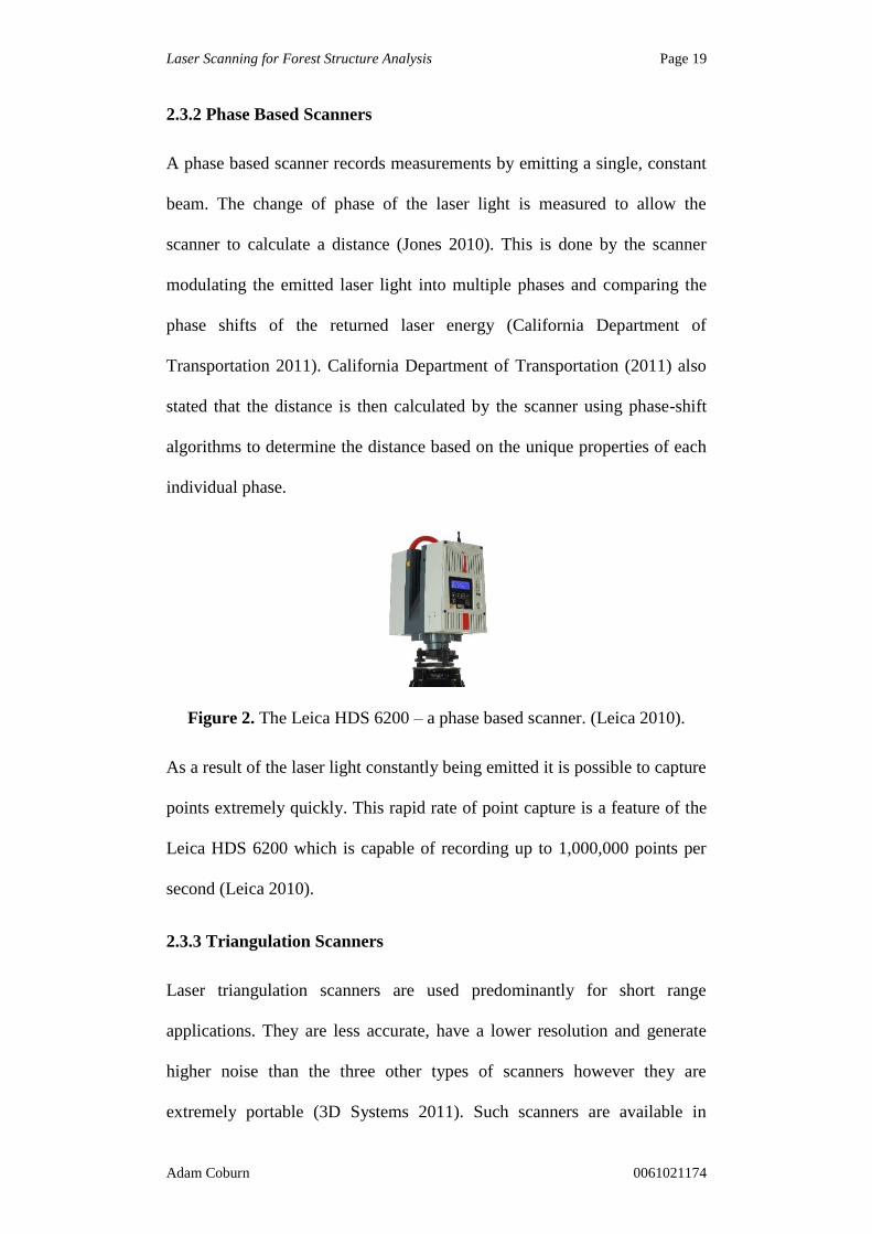
2.3.2 Phase Based Scanners
A phase based scanner records measurements by emitting a single, constant
beam. The change of phase of the laser light is measured to allow the
scanner to calculate a distance (Jones 2010). This is done by the scanner
modulating the emitted laser light into multiple phases and comparing the
phase shifts of the returned laser energy (California Department of
Transportation 2011). California Department of Transportation (2011) also
stated that the distance is then calculated by the scanner using phase-shift
algorithms to determine the distance based on the unique properties of each
individual phase.
Figure 2. The Leica HDS 6200 – a phase based scanner. (Leica 2010).
As a result of the laser light constantly being emitted it is possible to capture
points extremely quickly. This rapid rate of point capture is a feature of the
Leica HDS 6200 which is capable of recording up to 1,000,000 points per
second (Leica 2010).
2.3.3 Triangulation Scanners
Laser triangulation scanners are used predominantly for short range
applications. They are less accurate, have a lower resolution and generate
higher noise than the three other types of scanners however they are
extremely portable (3D Systems 2011). Such scanners are available in

Laser Scanning for Forest Structure Analysis Page 20
Adam Coburn 0061021174
handheld options and consequently require less preparation. They are also
less sensitive to ambient light.
Triangulation scanners measure distances, which allows them to create
points, by using a laser line or single laser point to scan across and object. A
sensor then detects the reflected light and calculates the distance from the
object to the scanner using trigonometric triangulation (3D Systems 2011).
For this to occur, the distance and angle between the sensor and laser source
must be known extremely precisely. These known parameters allow the
machine to identify the angle of the laser when reflected off the object and
detected by the sensor. Resultantly, a position can be calculated for the
scanned point.
2.3.4 Waveform Processing Scanners
Waveform processing scanners are also referred to as echo digitisation
scanners. These instruments use pulsed time-of-flight technology and
internal real-time waveform processing techniques to identify multiple
returns or reflections of the same signal pulse, resulting in the detection of
multiple objects (California Department of Transportation 2011).
Figure 3. The Riegl VZ-400 – a waveform processing scanner. (Reigl
2014).

Laser Scanning for Forest Structure Analysis Page 21
Adam Coburn 0061021174
Waveform processing scanners are also capable to measure points at an
extremely high rate. California Department of Transportation (2011)
identified that waveform processing scanners can possess a pulse rate of
300,000 as well as an echo detection capability of 15 returns per pulse. This
allows data collection rates to achieve, and potentially exceed, 1.5 million
points a second (California Department of Transportation 2011).
The main limitation of echo digitising scanners is the inability to
discriminate between returns of the same laser pulse. This is a result of
objects that are closely spaced. Figure 4 provides an example of such a
situation.
Figure 4. Multiple echo detection – (California Department of
Transportation 2011).

Laser Scanning for Forest Structure Analysis Page 22
Adam Coburn 0061021174
In Figure 4, “d” is the discrimination limit which is a function of laser
emitter and receiver operating parameters. California Department of
Transportation (2011) stated that returns from objects that are closer
together than the laser scanner’s multiple object discrimination limit will
create false points in the data. The problem of false points can be reduced
however it is beyond the scope of this dissertation.
2.4 Current Applications of Laser Scanners
Laser scanners have been around for approximately twenty years (SurvTech
Solutions 2014) allowing a multitude of their uses to be tested. Before the
equipment becomes staple use in an environment, it must be vigorously
tested to assess the suitability of the equipment to the application. Once
testing is completed and the results are satisfactory, the device can progress
from uncommon use in the area to common practice.
2.4.1 Engineering Applications
Within the engineering world terrestrial laser scanning has a multitude of
applications. Some of these require an extremely high accuracy while others
require an accuracy of lower standards. These categories have been divided
and explained below.
2.4.1.1 Strict High Accuracy Requirements
The accuracy required for engineering work is ±0.0091m horizontally and
±0.0061m vertically (California Department of Transportation 2006).
Resultantly an extremely accurate and precise instrument must be used. This
can greatly increase costs as some cheaper forms of equipment may not

Laser Scanning for Forest Structure Analysis Page 23
Adam Coburn 0061021174
meet the specifications required. Consequently they would not be suitable to
the task.
California Department of Transportation (2011) deemed that the following
applications require engineering level accuracy:
Pavement Analysis Scans
Roadway/pavement topographic surveys
Structures and bridge clearance surveys
Engineering topographic surveys
Deformation and monitoring surveys
As-built surveys
The data captured by these surveys is critically analysed and resultantly
must represent the real world as closely as possible.
2.4.1.2 Tasks of Lesser Accuracy
Tasks suitable to laser scanning requiring less accuracy include:
Corridor study and planning surveys
Earthwork surveys
Environment surveys
Sight distance analysis surveys
Urban mapping and modelling
This can be due to: working with loose materials, analysing moving objects
or conducting planning or modelling surveys (California Department of
Transportation 2011).

Laser Scanning for Forest Structure Analysis Page 24
Adam Coburn 0061021174
2.4.2 Non-Engineering Applications
A laser scanner has various uses outside of the engineering environment.
These applications range across various fields, utilise different types of
scanners and have varying accuracy standards.
Laser scanning has been effectively used to monitor coastal erosion. Rosser
et. al. (2005) analysed a coastal cliff face made up of hard rock. The cliff
was monitored over a period of 16 months and it was concluded that laser
can quantify cliff failures to a previously unobtainable precision.
Analysing cultural heritage is extremely important as it provides us with
information on the quality of the structure. By analysing the structure it is
possible to identify repairs that need to be conducted to help preserve the
object. Castagnetti et. al. (2012) observed the Cathedral of Modena and
were able to create a model that can be used for monitoring deformation.
The highly detailed data was also used to analyse structural integrity and
compute anomalies in structural geometry.
Crime scenes must be analysed to a high detail to ensure that correct
verdicts are reached by judge or jury. By utilising laser scanning to its full
potential, it is possible to create a virtual representation of a crime scene
allowing for detailed analysis. Agosto, Ajmar, Boccardo, Tonolo, & Lingua
(2008) identified that this virtual recreation can be more compelling for
juries and also allows for investigators to virtually ‘revisit’ a crime scene.
Forest analysis is a tedious process, requiring a large number of man hours.
Data must be recorded accurately and to a high detail. By using laser
scanning, Newnham et. al. (2012) concluded that laser scanning is well
Laser Scanning for Forest Structure Analysis Page 25
Adam Coburn 0061021174
suited to the application and has the potential to save time and increase
accuracy.
2.5 Forest Structure Analysis
Forest structures are analysed and recorded into a forest inventory. These
inventories detail important information about the structure and are an
investment to support current and future forest resource opportunities (BC
Forest Conversation 2013). BC Forest Conversation (2013) also states that
forest inventories are the primary source of information for determining
acceptable annual harvest levels while at the same time maintaining healthy
forests and healthy communities. The uses of a forest inventory reinforce its
need to be accurate and well documented.
2.5.1 Types of Inventories
Forest inventories, although large, are targeted to achieve a single purpose.
Resultantly there are multiple types of inventories. Food and Agriculture
Organisation of the United Nations Forestry Department (2014) identifies
eight types of forest inventory contained within two different categories.
The first category, harvesting, features pre-concession, logging planning and
management planning inventories. Management inventories make up the
second category and compile growth studies, biodiversity surveys, social
surveys, post-harvest and diagnostic sampling inventories.
2.5.2 Inventory Objectives
Eight types of inventories have been identified with each inventory designed
for a specific purpose. Consequently each inventory has its own objective.
However, ‘objectives must be quite clear irrespective of whether an

Laser Scanning for Forest Structure Analysis Page 26
Adam Coburn 0061021174
inventory is proposed for an existing forest management unit or for a new
concession’ (Food and Agriculture Organisation of the United Nations
Forestry Department 2014). Food and Agriculture Organisation of the
United Nations Forestry Department (2014) outline three specific guidelines
that should be considered when determining inventory objectives. The first
is that objectives need to be determined jointly by the people who will use
the results, not just by the inventory specialists. Second is that objectives
should be prioritised so that important information is not missed and that
unnecessary information is not collected. The final guideline is to ensure
that the inventory is both practicable and achievable. All aspects of the
inventory and the collecting process must be sound to ensure that time and
money is not wasted.
2.5.3 Components
Inventories are designed to achieve a specific purpose. Consequently the
key components of inventories vary. However some components are
applicable to a number of inventories reinforcing their importance.
Maniatis (2010) identified diameter at breast height (1.3m from forest
floor), height and wood density essential in determining carbon pools.
Measurement of tree diameters is an important variable for determining
forest growth, and care is needed to ensure that an accurate tree
measurement history is assembled (Food and Agriculture Organisation of
the United Nations Forestry Department 2014). The horizontal area of a tree
trunk is defined as the basal area and is calculated by converting the
diameter at breast height to an area.

Laser Scanning for Forest Structure Analysis Page 27
Adam Coburn 0061021174
When measuring tree height and resultantly volume, the structure is
assumed to be a cylinder and the volume is then determined. However
Brack (1999) outlined four types of tree volume and resultantly volume is
calculated dependant on the purpose. Biological volume is the volume of
stem with branches trimmed at the junction with the stem. Merchantable
volume excludes volume within irregularities of the bole shape caused by
normal growth as well as irregularities not part of natural growth. Gross
volume estimates include decayed and defective wood whereas net volume
excludes decayed and defective wood. Different purposes are calculated in
different ways, with some volumes requiring vigorous work with complex
formulae.
2.6 Laser Scanning of Forest Structures
The suitability of using laser scanning technology to analyse and monitor
forest structures has been assessed a number of times. Multiple studies have
been conducted, differing in both purpose and method with each study
increasing knowledge and understanding of using terrestrial laser scanning
to analyse forest structures.
Thies and Spiecker (2004) conducted a study which featured two
hypotheses. The first was that terrestrial laser scanning and the
corresponding data analysis is ready to be used in standardised forest
inventory sampling. The second outlined that data quality as well as
characteristics related to the technique of laser scanning widen the data base
for forest management applications and ecological investigations. With
regards to the first hypothesis, Thies and Spiecker (2004) concluded that the

Laser Scanning for Forest Structure Analysis Page 28
Adam Coburn 0061021174
technology allows for an accurate analysis and has a number of potential
possibilities. To establish this process, Thies and Spiecker (2004) stated that
robust models for data analysis as well as improvements in hardware
technology are required. By proving the second hypothesis, Thies and
Spiecker (2004) were able to show that repeated measurements at different
times but identical scanner positions can be compared directly which
eliminates human discrepancy when recording inventory data. Furthermore
it was identified that data acquisition and analysis is independent from
subjective influences of the measuring person. Lastly, and possibly the most
important finding, was that by using terrestrial laser scanning, a large data
pool is created which can be used for a vast number of investigations.
Newnham et al. (2012) observed not only the suitability of terrestrial laser
scanning within a vegetated environment, but also which type of scanner
was more suited to the application. Two time of flight scanners and two
phase based scanners were used for the study. One finding of this study was
that ‘time of flight instruments, at the time, provided the best
characterisation of vegetation structure, mainly in the upper parts of the
canopy, where multiple beam interceptions are not accommodated well by
the phase-shift scanners’ (Newnham et al. 2012).
Burt et al. (2013) analysed the ability to construct tree members using TLS
and 3D modelling. The study also assessed allometric relationships which
relate DBH and height to biomass. This is a key factor to inventory
estimates of forest biomass. After assessing multiple structures, it was
concluded that it was possible to generate tree reconstruction to within 10%
of the actual volume of the tree. The key limitation was of the study was

Laser Scanning for Forest Structure Analysis Page 29
Adam Coburn 0061021174
that ‘inducing a 1cm global registration error leads to an 8.8% increase in
total volume’ (Burt et al. 2013). By combining this study with previous
studies, Burt et al. (2013) believe that there is a possibility to provide a
number of opportunities ranging from independent biomass estimation
through to validation of allometric scaling.
Cote et al. (2009) designed a system to accurately reconstruct trees from
TLS. This system was designed to help with the various forms of noise that
is generated when scanning forest structures. This includes both wind and
the smaller tree constituents such as branches, twigs and foliage. Data
obtained from the scans was found to be usable and provided an appropriate
representation of the structure. Once the reconstruction system was applied,
evaluations were performed on the new data. The outcome of the study was
that ‘the results of these evaluations confirm the appropriateness of the
proposed tree reconstruction model for the generation of structurally and
radiatively faithful copies of existing plant and canopy architectures’ (Cote
et al. 2009).
Raumonen et al. (2013) followed in the footsteps of Cote et al. (2009) and
analysed the success of reconstructing tree structures from laser scanner
data. The method that was developed and assessed involved reconstructing
the visible parts of the tree by creating a flexible cylinder model of the tree.
These cylinders also extended into the branch structure of the tree to
reconstruct the whole tree not including vegetation. The new technique was
determined to be successful in constructing trees from laser scanner data and
allowed for easy identification of multiple tree attributes.

Laser Scanning for Forest Structure Analysis Page 30
Adam Coburn 0061021174
2.7 Conclusion
This chapter has identified and discussed the literature relevant to the
research topic. Background information on scanners and their current
applications have been highlighted. Alongside this, the need for forest
analysis and basic inventory components were discussed. Furthermore, laser
scanning’s current use within a forest structure was brought forward.

Laser Scanning for Forest Structure Analysis Page 31
Adam Coburn 0061021174
Chapter 3 - Methodology
3.1 Introduction
This chapter will identify the processes undertaken to fulfil the research
aim. It will feature:
Study Area
Equipment
Field Procedures
Post Processing
Comparison Methods
3.2 Study Area
The study area selected is located on the eastern side of Picnic Point,
Toowoomba.
Figure 5. Toowoomba’s location within Queensland
(Toowoomba Motor Village 2014)
An estimation of the size of the area has been calculated using satellite
photos. These estimations resulted in the area being approximately 6700m2.

Laser Scanning for Forest Structure Analysis Page 32
Adam Coburn 0061021174
This site is also moderately steep as a result of being on the side of a
mountain. The location features areas of both dense and open canopy. Areas
on the ground are also open as well as fairly populated with tree structures.
Figure 6. Satellite view of the study area (Google Earth 2014)
The varying terrain and densities combined with varying tree heights and
thicknesses allows for unbiased testing. Twenty individual structures of
varying height and diameter will be analysed. The fluctuating measurements
will assist in removing consistent errors that may occur.
Figure 7. One section of the area being analysed.

Laser Scanning for Forest Structure Analysis Page 33
Adam Coburn 0061021174
3.3 Equipment
The FARO Focus 3D laser scanner has been used in this study. This scanner
is a phased based scanner capable of recording 976,000 points per second.
When properly calibrated, the Focus 3D records these points with an
accuracy of +/- 2mm. Alongside the scanner twelve reference spheres
(140mm diameter) were used to assist in registration.
To record data using traditional methods a Laser Tech Inc. Tru Pulse 360°
distometer was used. Such an instrument is able to calculate vertical height
on-the-fly requiring no calculations during data acquisition or post
processing. Alongside this instrument a flexible tape measure was used to
locate breast height and measure the DBH.
It has been assumed that all equipment is correctly calibrated as performing
such a task is beyond the scope of this research.
3.4 Field Procedures
3.4.1 Laser Scans
A total of seventeen scans were conducted with the field of view ranging
from 100 to 360 degrees. These scans were completed over two days. Both
days were slightly overcast and 25°C.
The largest of the files are the 360 degree scans which took just under ten
minutes to complete. These scans captured approximately 170 million
points with scans of smaller fields of view taking less time and making
fewer measurements. Alongside the points, the Focus 3D also captures

Laser Scanning for Forest Structure Analysis Page 34
Adam Coburn 0061021174
photos of the area scanned. These photos are overlayed onto the point
clouds to create a real-world view of the data.
Figure 8. The FARO Focus 3D conducting a scan.
The scan locations were planned to ensure minimal blind spots. Across the
two days, scanning took roughly twelve hours.
Figure 9. Scan locations within the study area.

Laser Scanning for Forest Structure Analysis Page 35
Adam Coburn 0061021174
Scans are aligned to one another by using reference spheres provided with
the scanner. These spheres are 140mm in diameter and feature special
reflective properties, allowing them to be detected by the software. The
scans are aligned by subsequent scans featuring spheres in the same
location. A common point is established and the scans can be registered. To
do this at least three spheres must be common between scans. Once scans
are registered a cluster is created (Appendix 3).
Twelve reference spheres were used for this study. Consequently spheres
had to be moved around the study area as scans were completed. This was
due to the large study area and the limited number of spheres. This did not
cause any failures with registration however the cluster from the first day
could not be registered with the cluster from the second day. The data
analysis was not affected by this complication.
3.4.2 Traditional Analysis
Forest inventory data must be collected using the current and traditional
methods to assess the suitability of the laser scanner. An assessment needs
to be made about the quality and size of the tree. To do this the following
information is collected using the described technique. This data took
approximately two hours to identify.
3.4.2.1 Tree Height
The distometer used is able to calculate vertical height of an object. To
achieve this three measurements are made. The first is to sight the object
and calculate the distance to the object. Afterwards an angle is sighted to the

Laser Scanning for Forest Structure Analysis Page 36
Adam Coburn 0061021174
top and bottom of the tree with simple trigonometry calculating the vertical
distance.
3.4.2.2 Diameter at Breast Height
The DBH is calculated by first marking a point on the tree 1.3m from the
forest floor. A tape is then wrapped around the trunk at this height to obtain
the circumference. This can be done to a higher accuracy by marking
multiple points around the tree at the same height. Once the circumference
is calculated, dividing the value by Pi will return the DBH.
3.4.2.3 Volume
Tree volume can be easily calculated by assuming the structure is a perfect
cylinder. Multiplying the basal area by the height gives the volume of the
structure.
3.5 Post Processing
3.5.1 Scan Analysis
FARO Scene is software provided by FARO used to analyse scans
conducted with their equipment. This software allows the user to analyse the
generated point cloud. It is also possible to overlay colour photographs on
these point clouds to achieve a realistic view.
These files containing both point clouds and photos are very large. Once
registration is completed the files become even larger. All scanned data
collected and processed was in excess of 78GB. Consequently an extremely
powerful computer had to be used. This was an overclocked desktop
computer featuring 16GB of RAM and an i7-4770K CPU. Such a powerful

Laser Scanning for Forest Structure Analysis Page 37
Adam Coburn 0061021174
computer allowed registration to be completed in one hour. A further thirty
minutes was required to identify tree characteristics.
Once the cluster is created through registration, it is possible to overlay the
captured photos onto the measured points. This allows for an accurate visual
representation of the cluster, rather than a black and white point cloud.
These photos are overlayed in three ways, identified as: Quick view, Planar
view and 3D view.
3.5.1.1 Quick View
The quick view overlay provides a view from the position of the scanner.
The photos are wrapped around the position of the scanner, allowing for 360
degree rotation around the view point. The limitation with this view is that
high places, namely the tops of trees, become distorted when the scale is
altered to view these high up places. The advantage of this view is the detail
provided when performing measurements. When conducting multiple
measurements, distances for each measurement are detailed, as well as a
vertical and horizontal distance from the starting point. A large scale and
small scale example are provided in Appendix 4, alongside a measurement
example.
3.5.1.2 Planar View
The planar view also provides a view from the position of the scanner. The
difference it has from the quick view is that the photos are wrapped to form
a flat, panoramic photo. This greatly minimises distortion when viewing
high places as there is no distortion when altering scale. Consequently the
top of structures can be interpreted easily, allowing for consistent

Laser Scanning for Forest Structure Analysis Page 38
Adam Coburn 0061021174
measurements. This view also identifies the location of other scans within
the same cluster. Resultantly it is possible to identify where in the cluster
the structure is and can also assist when trying to return to the individual
structure. The disadvantage to this view is that less detail is provided when
measuring objects. Unlike the quick view, only a total distance is given,
rather than the distance of each individual measurement. A horizontal and
vertical distance is still provided from the first to last measurement. Refer to
Appendix 5 for a small scale image and a measurement example.
3.5.1.3 3D View
The 3D View is used to compile the cluster. The photos are overlayed onto
the scan points, however any areas that cannot be overlayed onto points are
left blank. It is useful when determining the data each scan was able to
identify. Another advantage of this view is that the viewpoint is not limited
to the location of the scanner. However when moving through the point
cloud the data must reload each time a movement is made, clogging the
system. Resultantly obtaining data using this technique is time consuming.
Of these, the quick and planar views will be used to analyse tree structures.
These two views provide enough manipulation to allow the structures to be
analysed to a high degree. Resultantly DBH and height can be calculated.
3.5.2 Traditional Data Analysis
The traditionally collected data only provides the circumference at breast
height. Before processing can occur this measurement must be converted to
diameter for all structures. Completing all conversions and documenting the
data obtained took approximately two hours.
Laser Scanning for Forest Structure Analysis Page 39
Adam Coburn 0061021174
3.6 Data Comparison
To assess the suitability of laser scanning in capturing and analysing forest
structures, a comparison between scanned and traditionally collected data
must be performed.
To execute such a task twenty trees will be analysed. These structures will
vary in height, shape and diameter to ensure the outcome is unbiased.
Height and DBH will be determined so that volume can be calculated. The
volume is calculated by first determining the basal area. The basal area is
then multiplied by the height of the structure.
Data obtained using the quick and planar views will be compared to the
traditional method. An average of the two methods will also be calculated
and compared to the traditional data to identify which option is most
suitable.
3.7 Conclusion
This chapter identified the methods that will be used to fulfil the research
aims. The study area and equipment were identified. Methods used to
capture and analyse the data were discussed. Methods used to ensure an
accurate comparison were also highlighted.

Laser Scanning for Forest Structure Analysis Page 40
Adam Coburn 0061021174
Chapter 4 – Results
4.1 Introduction
This chapter will present the data acquired using the two methods.
Differences between the various data forms will also be identified.
4.2 Traditional Data
Traditional Data
Tree # Height (m) DBH (m) Basal Area (m2) Volume (m3)
Tree 1 9.2 0.282 0.062 0.0573
Tree 2 9.9 0.393 0.121 1.201
Tree 3 9 0.309 0.075 0.0674
Tree 4 4.9 0.589 0.272 1.334
Tree 5 12.2 0.703 0.388 4.739
Tree 6 5.9 0.579 0.263 1.554
Tree 7 11.9 0.468 0.172 2.045
Tree 8 10.5 0.503 0.199 2.085
Tree 9 10.8 0.344 0.093 1.002
Tree 10 8.9 0.675 0.357 3.181
Tree 11 7.1 0.616 0.298 2.114
Tree 12 7.1 0.417 0.136 0.969
Tree 13 11.5 0.608 0.290 3.337
Tree 14 12.1 0.573 0.258 3.118
Tree 15 11 0.557 0.244 2.679
Tree 16 9.3 0.417 0.136 1.269
Tree 17 3 0.427 0.143 0.428
Tree 18 13.4 0.296 0.069 0.922
Tree 19 4.5 0.449 0.158 0.712
Tree 20 5.9 0.242 0.046 0.271
Table 1. Data obtained from traditional methods.

Laser Scanning for Forest Structure Analysis Page 41
Adam Coburn 0061021174
4.3 Scanned Data
Quick View
Tree # Height (m) DBH (m) Basal Area (m2) Volume (m3)
Tree 1 9.378 0.252 0.050 0.467
Tree 2 10.003 0.371 0.108 1.081
Tree 3 9.371 0.271 0.058 0.540
Tree 4 5.112 0.554 0.241 1.232
Tree 5 12.473 0.664 0.346 4.317
Tree 6 6.303 0.533 0.223 1.406
Tree 7 12.046 0.387 0.118 1.416
Tree 8 10.658 0.454 0.162 1.724
Tree 9 10.939 0.242 0.046 0.503
Tree 10 8.940 0.543 0.231 2.069
Tree 11 7.16 0.459 0.165 1.184
Tree 12 7.407 0.378 0.112 0.831
Tree 13 11.627 0.550 0.237 2.761
Tree 14 12.19 0.547 0.235 2.863
Tree 15 11.381 0.494 0.192 2.180
Tree 16 9.426 0.331 0.086 0.811
Tree 17 3.012 0.397 0.124 0.373
Tree 18 13.874 0.216 0.037 0.508
Tree 19 4.749 0.412 0.133 0.633
Tree 20 6.165 0.233 0.043 0.263
Table 2. Quick view tree measurements.
Planar View
Tree # Height (m) DBH (m) Basal Area (m2) Volume (m3)
Tree 1 9.420 0.226 0.040 0.378
Tree 2 9.789 0.353 0.098 0.958
Tree 3 9.298 0.281 0.062 0.576
Tree 4 5.061 0.529 0.220 1.112
Tree 5 12.375 0.647 0.329 4.067
Tree 6 6.339 0.516 0.209 1.325
Tree 7 12.105 0.378 0.112 1.358

Laser Scanning for Forest Structure Analysis Page 42
Adam Coburn 0061021174
Tree 8 10.628 0.435 0.149 1.579
Tree 9 10.962 0.248 0.048 0.529
Tree 10 8.941 0.567 0.252 2.256
Tree 11 7.128 0.500 0.196 1.399
Tree 12 7.367 0.365 0.105 0.770
Tree 13 11.554 0.541 0.230 2.655
Tree 14 12.164 0.519 0.211 2.572
Tree 15 11.399 0.516 0.209 2.383
Tree 16 9.499 0.320 0.080 0.764
Tree 17 3.005 0.394 0.122 0.366
Tree 18 13.868 0.197 0.030 0.422
Tree 19 4.701 0.409 0.131 0.617
Tree 20 6.204 0.229 0.041 0.255
Table 3. Planar view tree measurements.
Average
Tree # Height (m) DBH (m) Basal Area (m2) Volume (m3)
Tree 1 9.399 0.239 0.045 0.421
Tree 2 9.896 0.362 0.103 1.018
Tree 3 9.335 0.276 0.060 0.558
Tree 4 5.087 0.542 0.230 1.171
Tree 5 12.424 0.656 0.337 4.191
Tree 6 6.321 0.525 0.216 1.365
Tree 7 12.076 0.383 0.115 1.387
Tree 8 10.643 0.445 0.155 1.651
Tree 9 10.951 0.245 0.047 0.516
Tree 10 8.941 0.555 0.242 2.162
Tree 11 7.144 0.480 0.180 1.289
Tree 12 7.387 0.372 0.108 0.800
Tree 13 11.591 0.546 0.234 2.707
Tree 14 12.177 0.533 0.223 2.716
Tree 15 11.390 0.505 0.200 2.280
Tree 16 9.463 0.326 0.083 0.787
Tree 17 3.009 0.396 0.123 0.369
Tree 18 13.871 0.207 0.033 0.464
Tree 19 4.725 0.411 0.132 0.625

Laser Scanning for Forest Structure Analysis Page 43
Adam Coburn 0061021174
Tree 20 6.185 0.231 0.042 0.259
Table 4. Average tree measurements from scanned data.
4.4 Variations
From these measurements, variances can be calculated between the three
types of scan measurements and the traditional method.
Figure 10. Variances in height between scanned data and traditional.
Height
Quick View Planar Average
Mean 0.206 0.185 0.196
Std Dev 0.127 0.146 0.133
Table 5. Mean height variances and standard deviations.
-0.200
-0.100
0.000
0.100
0.200
0.300
0.400
0.500
0.600
1 2 3 4 5 6 7 8 9 10 11 12 13 14 15 16 17 18 19 20
Height
Planar
Quick
Average
Tree No.
Dif
fere
nce

Laser Scanning for Forest Structure Analysis Page 44
Adam Coburn 0061021174
Figure 11. Variances in DBH between scanned data and traditional.
DBH
Quick View Planar Average
Mean -0.058 -0.064 -0.061
Std Dev 0.037 0.028 0.032
Table 6. Mean DBH variances and standard deviations.
Figure 12. Variances in basal area between scanned data and traditional.
-0.180
-0.160
-0.140
-0.120
-0.100
-0.080
-0.060
-0.040
-0.020
0.000
1 2 3 4 5 6 7 8 9 10 11 12 13 14 15 16 17 18 19 20
DBH
Planar
Quick
Average
Tree No.
Dif
fere
nce
(m
)
-0.140
-0.120
-0.100
-0.080
-0.060
-0.040
-0.020
0.000
1 2 3 4 5 6 7 8 9 10 11 12 13 14 15 16 17 18 19 20
Basal Area
Planar
Quick
Average
Tree No.
Dif
fere
nce
(m2

Laser Scanning for Forest Structure Analysis Page 45
Adam Coburn 0061021174
Basal Area
Quick View Planar Average
Mean -0.042 -0.045 -0.044
Std Dev 0.033 0.025 0.028
Table 7. Mean basal area variances and standard deviation.
Figure 13. Variances in volume between scanned data and traditional.
Volume
Quick View Planar Average
Mean -0.352 -0.393 -0.374
Std Dev 0.292 0.254 0.266
Table 8. Mean volume variances and standard deviation.
Percentage
Tree # Height DBH Basal Area Volume
Tree 1 2.163 -15.159 -28.020 -26.464
Tree 2 -0.040 -7.914 -15.203 -15.237
Tree 3 3.717 -10.610 -20.095 -17.125
Tree 4 3.806 -8.045 -15.442 -12.224
Tree 5 1.836 -6.818 -13.172 -11.578
Tree 6 7.136 -9.463 -18.031 -12.182
Tree 7 1.475 -18.254 -33.177 -32.191
-1.200
-1.000
-0.800
-0.600
-0.400
-0.200
0.000
1 2 3 4 5 6 7 8 9 10 11 12 13 14 15 16 17 18 19 20
Volume
Planar
Quick
Average
Tree No.
Dif
fere
nce
(m3

Laser Scanning for Forest Structure Analysis Page 46
Adam Coburn 0061021174
Tree 8 1.362 -11.618 -21.886 -20.822
Tree 9 1.394 -28.732 -49.209 -48.501
Tree 10 0.455 -17.755 -32.358 -32.051
Tree 11 0.620 -22.150 -39.394 -39.018
Tree 12 4.042 -10.908 -20.627 -17.418
Tree 13 0.787 -10.275 -19.495 -18.862
Tree 14 0.636 -6.974 -13.462 -12.911
Tree 15 3.545 -9.343 -17.812 -14.898
Tree 16 1.747 -21.940 -39.066 -38.001
Tree 17 0.283 -7.276 -14.023 -13.779
Tree 18 3.515 -30.243 -51.340 -49.629
Tree 19 5 -8.537 -16.346 -12.163
Tree 20 4.822 -4.512 -8.821 -4.424
Mean 2.415 -13.326 -24.349 -22.474
Table 9. Percentage variances between scanned average and traditional.
Figure 14. Variation as a percentage between traditional and scanned data
average.
-60
-50
-40
-30
-20
-10
0
10
20
1 2 3 4 5 6 7 8 9 10 11 12 13 14 15 16 17 18 19 20
Discrepancies (%)
Height
DBH
BasalArea
Volume
Tree No.
Dif
fere
nce
(%
)

Laser Scanning for Forest Structure Analysis Page 47
Adam Coburn 0061021174
4.4 Conclusion
This chapter has presented the data obtained for this study. The data was
obtained using traditional methods as well as laser scanning. Both methods
analysed height, DBH, basal area and volume.

Laser Scanning for Forest Structure Analysis Page 48
Adam Coburn 0061021174
Chapter 5 – Discussion
5.1 Introduction
The data that was obtained using traditional methods has been analysed to
calculate DBH, basal area and volume of twenty tree structures. The same
procedures have been followed to allow the same to be done for the data
collected using the FARO Focus 3D.
The scanned data has been analysed using two methods made available by
the software used. FARO Scene allows for measurements to be made using
both a quick view and a planar view. These two methods, along with an
average, will be analysed alongside the traditional methods to analyse the
suitability of using laser scanning to analyse forest structures.
5.2 Quick View Analysis
The quick view data is outlined in Table 2 with the variances provided in
Figures 10 through 13.
5.2.1 Height
The mean height variation of the twenty trees identifies that the quick view
data overestimates the height of each tree by 211mm. At first glance this is
quite a discrepancy however there are factors that condone this error. The
first is that the distometer used can only make measurements to the nearest
100mm. Such a measurement already reduces the potential error by almost
half. Secondly, the distometer is susceptible to human error at a higher
degree than the scan analysis. To accurately align the distometer with the

Laser Scanning for Forest Structure Analysis Page 49
Adam Coburn 0061021174
measurement point, hands must be held steady and the eyes of the user
would need to provide perfect vision. A slight movement from the required
point to be measured combined with the 100mm accuracy can drastically
alter the distance measured. Alongside this, the distometer can only measure
vertical heights. If a tree is not completely straight, error is introduced to the
measurement.
Figure 15. Vertical height error.
An angle as small as twenty degrees can introduce a height difference of
600mm as seen in Figure 15. From the analysed data, the largest variance in
height is 474mm on tree #18. Although the angle to the measured point is
not great (Figure 16), the height of the tree can easily provide this
discrepancy. As the height increases, so too does the variation in vertical
height if the angle of deviation remains consistent. In contrast, the smallest
difference is 12mm which was measured on tree 17.
10m
10m
20o
9.4m
70o
Laser Scanning for Forest Structure Analysis Page 50
Adam Coburn 0061021174
Figure 16. Tree #18, the largest quick view variation.
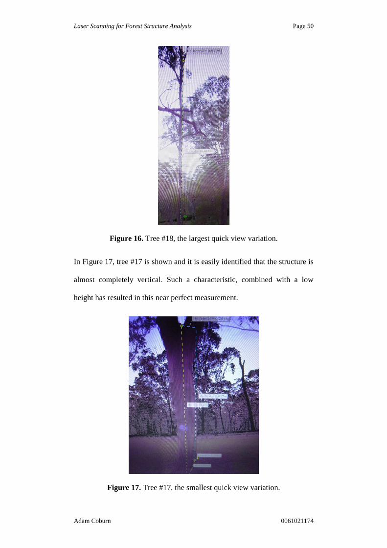
In Figure 17, tree #17 is shown and it is easily identified that the structure is
almost completely vertical. Such a characteristic, combined with a low
height has resulted in this near perfect measurement.
Figure 17. Tree #17, the smallest quick view variation.

Laser Scanning for Forest Structure Analysis Page 51
Adam Coburn 0061021174
When assessing the mean and standard deviation of the quick view
variations, the data is positive. The mean identifies that the quick view
measurements overestimate the tree height by 206mm. However based on
previous statements, it is possible that the distometer underestimates the
height by this measurement. Reinforcing this idea is the standard deviation
of 127mm. Such a distance is near the measurement accuracy of the
distometer without introducing human error. Resultantly, the data suggests
that FARO Scene’s quick view measurements can accurately record tree
height data, possibly to a higher standard than that of traditional methods.
5.2.2 Diameter at Breast Height
As opposed to height measured with the quick view, the DBH of all twenty
trees is smaller than the traditional method. Of the data, all bar three
measurements fall outside a 100mm difference with the mean variation
calculated as -58mm. Although it is difficult to suggest the reasoning behind
this uniform discrepancy, errors in photo overlay could be a likely cause.
When measurements were made from one edge of the tree to the other, the
results were occasionally extremely wrong. One measurement returned a
DBH in excess of sixteen metres. This resulted in selecting a point that was
not part of the tree structure, although with an increased scale it appeared it
was. The distortion in the increased scale resulted in photo overlays
misrepresenting the point clouds and consequently negatively impacting
measurements. Tree #20 had the smallest error when calculating DBH with
the calculation 9mm less than that of the traditionally collected data.
The worst measurement was made on structure 11, with the measurement
returning a value 157mm smaller than the traditional method.

Laser Scanning for Forest Structure Analysis Page 52
Adam Coburn 0061021174
Figure 18. Tree #20, the smallest DBH variation.
Figure 19. Tree #11, the largest DBH variation.
By analysing both Figure 18 and 19, it is easy to identify the distortion
present in Figure 19 as well as the lack of in Figure 18. There is also shadow
present on one edge of the tree in Figure 19 which may have caused a
misinterpretation of the structure’s limits. Much like the height
measurements, there is an error consistency. In this case it is an
underestimation of each structure’s DBH. With a mean of 58mm and a

Laser Scanning for Forest Structure Analysis Page 53
Adam Coburn 0061021174
standard deviation of 37mm, it is quite a significant error. However the
current method of obtaining DBH is not always accurate. While the quick
view measurement allows for a straight line to be drawn across the tree,
parallel to the ground, such a measurement is not possible in the field. A
tape measure must be wrapped around the tree and is susceptible to multiple
errors. This includes: not being parallel to the ground, not being at 1.3m
from the ground, fluctuations in the tape as it is wrapped around the tree, the
tape not resting perfectly against the tree edges and if the measurement is
made on a hill, the tape may not be representative of a flat plane that is 1.3m
from the forest floor on the highest side. Such a high number of possible, if
not probable errors suggests that much like the case with height, the scanner
measurements, although they seem incorrect, reflect the true measurement
of the tree to a greater degree than the traditional methods.
5.2.3 Volume
To calculate the volume of the tree, the DBH is converted to area. Such an
area is known as the basal area and is multiplied by the height of the tree to
determine the tree volume. The largest variation between quick view
analysis and traditional analysis was identified on tree #10. Although this
structure had an excellent height measurement (+40mm) and the DBH
calculation was not the worst in the population (25mm better than #11), the
height of the tree caused the difference to become significant. The volume
variation of tree #10 is 1.112m3 which is 35% of the traditional volume.
However by analysing the problems associated with this calculation as well
as the remaining volume variances, it appears this measurement is an
outlier. Although the height is good and well within the standard deviation

Laser Scanning for Forest Structure Analysis Page 54
Adam Coburn 0061021174
and below the mean, the DBH is the exact opposite. The DBH measurement
for this structure is 227% of the mean variation and three and a half times
larger than the standard deviation. This miscalculation combined with a tree
of such a large height easily explains the discrepancy between the two
measurement methods.
Tree #20 has a DBH calculation that is near identical to the traditional
method and has resulted in the volume differing by a mere 0.008m3. The
underestimate of the DBH and the overestimate of the height has resulted in
this near exact measurement.
The mean volume variation amongst all twenty measurements is an
underestimation of 0.352m3. However if structure #10 and #11 are removed
(the two outliers), this is reduced to 0.278m3 which is an immense
improvement, a 21% reduction. Resultantly, it can be stated that if the two
outliers are removed, the quick view measurements underestimate tree
volume by 0.278m3. This figure represents 21% of average tree volume
(1.328m3) when the outliers are again removed.
5.3 Planar View
The planar view data is outlined in Table 3 with the variances provided in
Figures 10 through 13.
5.3.1 Height
As was the case with the quick view measurements, tree #18 featured the
greatest difference to the measurement made by traditional methods. The
planar view error was a 468mm excess, 6mm less than the error identified in

Laser Scanning for Forest Structure Analysis Page 55
Adam Coburn 0061021174
the quick view measurement. Again this is likely due to the large height of
the tree combined with an offset angle.
Continuing this trend, the closest representation was the measurement on
tree #17. This error was 5mm, 7mm less than the quick view. Such a
measurement can be explained by the straightness of the tree as well as its
low height.
The average difference (185mm) is also less than the quick view average
(206mm). Such a result suggests that the planar view is better suited to
measuring height than the quick view.
5.3.2 Diameter at Breast Height
Reflective of quick view measurements, the largest DBH error was on tree
#11. However this error (116mm) was 41mm less than the quick view error
(157mm). This is an extensive difference, constituting a 26% improvement.
Furthermore, the smallest difference is 13mm and much like the quick view,
has been made on tree #20. The difference of 4mm between the two
measurements is insignificant.
It should be noted however, that the average difference between planar and
traditional measurement (64mm) is 6mm higher than the quick view average
(58mm), even though the largest DBH discrepancy is 41mm less. Another
observation to note is that tree #10 and #11 are not such obvious outliers as
they are in the quick view data. However, if the two aforementioned outliers
are removed from the planar and quick view data sets, this average is
reduced to 58mm and 48mm respectively. Although this does not change
the data to an extensive degree, it does suggest that the planar view may

Laser Scanning for Forest Structure Analysis Page 56
Adam Coburn 0061021174
provide a better representation of DBH than what is provided by the quick
view measurements.
5.3.3 Volume
The average volume discrepancy observed when using the planar view for
measurements is -0.393m3. When compared to the quick view average of
-0.352m3, this is a slight difference (0.041m3). However if, like in the
previous section, the two quick view outliers are removed, the quick and
planar view average becomes -0.346m3 and -0.278m3 respectively.
Consequently the difference in average volume becomes 0.068m3, a 70%
increase. Such data suggests that the quick view is more appropriate if
calculating volume.
5.4 Average of Quick and Planar Measurements
For this study, two independent measurements have been made to calculate
two factors. The independent measurements, DBH and height, are
manipulated to identify basal area and volume. In both independent cases, it
was easily identified which measurement closely reflected that of the
traditional method. When referring to height, planar view measurements
were similar to the traditional results. In the case of DBH, the measurements
made within quick view better reflected the traditional measurements.
Such a result does not identify which method is more suited to such an
application. However once volume is calculated, it is evident that the quick
view measurements hold the smallest margin between itself and traditional
analysis. In contrast, the average may better reflect the measurement

Laser Scanning for Forest Structure Analysis Page 57
Adam Coburn 0061021174
because planar view was more suited to height calculation and quick view to
DBH.
Planar Height & Quick DBH
Tree # Height (m) DBH (m) Basal Area (m2) Volume (m3)
Tree 1 9.420 0.252 0.050 0.470
Tree 2 9.789 0.371 0.108 1.058
Tree 3 9.298 0.271 0.058 0.536
Tree 4 5.061 0.554 0.241 1.219
Tree 5 12.375 0.664 0.346 4.283
Tree 6 6.339 0.533 0.223 1.414
Tree 7 12.105 0.387 0.118 1.423
Tree 8 10.628 0.454 0.162 1.720
Tree 9 10.962 0.242 0.046 0.504
Tree 10 8.941 0.543 0.231 2.069
Tree 11 7.128 0.459 0.165 1.179
Tree 12 7.367 0.378 0.112 0.826
Tree 13 11.554 0.550 0.237 2.744
Tree 14 12.164 0.547 0.235 2.857
Tree 15 11.399 0.494 0.192 2.184
Tree 16 9.499 0.331 0.086 0.817
Tree 17 3.005 0.397 0.124 0.372
Tree 18 13.868 0.216 0.037 0.508
Tree 19 4.701 0.412 0.133 0.626
Tree 20 6.204 0.233 0.043 0.264
Table 10. Volume calculated using planar height and quick DBH.
Laser Scanning for Forest Structure Analysis Page 58
Adam Coburn 0061021174
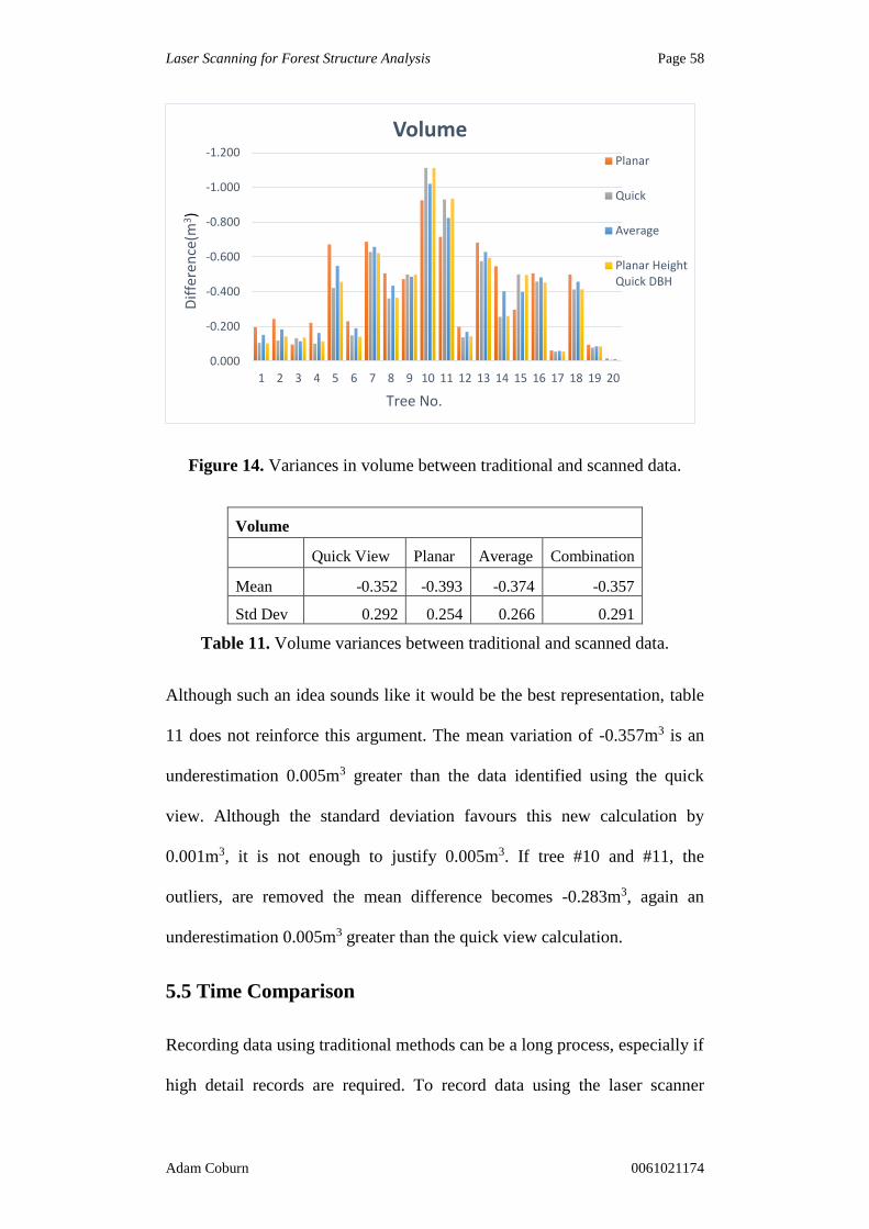
Figure 14. Variances in volume between traditional and scanned data.
Volume
Quick View Planar Average Combination
Mean -0.352 -0.393 -0.374 -0.357
Std Dev 0.292 0.254 0.266 0.291
Table 11. Volume variances between traditional and scanned data.
Although such an idea sounds like it would be the best representation, table
11 does not reinforce this argument. The mean variation of -0.357m3 is an
underestimation 0.005m3 greater than the data identified using the quick
view. Although the standard deviation favours this new calculation by
0.001m3, it is not enough to justify 0.005m3. If tree #10 and #11, the
outliers, are removed the mean difference becomes -0.283m3, again an
underestimation 0.005m3 greater than the quick view calculation.
5.5 Time Comparison
Recording data using traditional methods can be a long process, especially if
high detail records are required. To record data using the laser scanner
-1.200
-1.000
-0.800
-0.600
-0.400
-0.200
0.000
1 2 3 4 5 6 7 8 9 10 11 12 13 14 15 16 17 18 19 20
VolumePlanar
Quick
Average
Planar HeightQuick DBH
Tree No.
Dif
fere
nce
(m3)

Laser Scanning for Forest Structure Analysis Page 59
Adam Coburn 0061021174
approximately twelve hours was required. An extra hour was required to
process all scans before data analysis. Once this was completed the data was
readily available to process. Obtaining the required measurements using
both views took roughly thirty minutes to calculate and record.
Observing the twenty trees using contemporary methods required four hours
of work. Two hours to measure trees in the field and then another two of
post processing which included calculations and data entry. In total the
scanned analysis took thirteen and a half hours whereas the traditional
analysis took only four hours. A difference of nine and a half hours is quite
large and suggests that scanning is impractical. However if the quantity of
data is compared the outcome changes. In three hours traditional methods
could only analyse twenty trees. Although scanning took longer, data is
available for every individual structure within the study area. The amount of
information that can be extracted from the scan is only limited to the size of
the scan. Adding to this, the data can be analysed at any time. When using
traditional methods the only data that can be analysed is what has been
recorded in the field. Although photos can allow for later analysis, no
measurements can be executed and if photos do not fulfil the requirements it
may be necessary to return to the site.
Such results convey that laser scanning is a more efficient way to capture
data. With improved scanning techniques and planning, data capture time
could be limited to only slightly longer than the total time of the scans. This
study used eighteen scans at approximately ten minutes each although the
total capture time took twelve hours. This leaves nine hours unaccounted for
but in this instance it was associated to inexperience of the operator.

Laser Scanning for Forest Structure Analysis Page 60
Adam Coburn 0061021174
Although the time taken could be improved in both instances, there is
greater room for improvement in the scanning procedures. A true
comparison cannot be made unless the same number of individual trees are
analysed using both methods but observations on the techniques used in this
study propose that laser scanning is more efficient.
5.6 Conclusion
FARO Scene is software used to make measurements on scan point clouds.
This can be done in the various views provided which include a quick,
planar and 3D view. Using the point clouds observed, the quick and planar
views were used to calculate tree height and DBH. This data was then
manipulated to determine the basal area and volume for twenty trees within
the aforementioned study area.
It was identified that the quick view was more suited to calculating DBH
than the planar view. In the case of tree height, the planar view was deemed
more appropriate. These results were reached by comparing the
measurements made to data that was recorded using traditional forest data
collection techniques. An average of the two views, as well as a
combination of the two was also compared to the traditional data. However
the data obtained using only the quick view best suited the traditional
analysis.
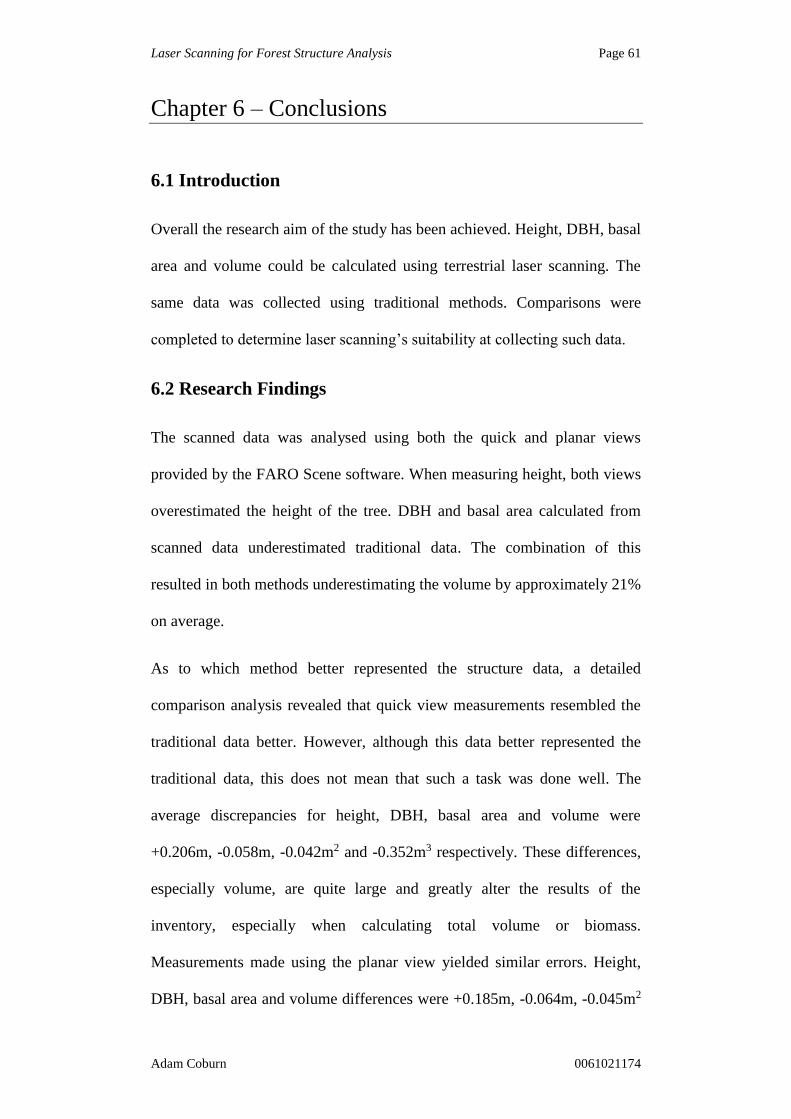
Laser Scanning for Forest Structure Analysis Page 61
Adam Coburn 0061021174
Chapter 6 – Conclusions
6.1 Introduction
Overall the research aim of the study has been achieved. Height, DBH, basal
area and volume could be calculated using terrestrial laser scanning. The
same data was collected using traditional methods. Comparisons were
completed to determine laser scanning’s suitability at collecting such data.
6.2 Research Findings
The scanned data was analysed using both the quick and planar views
provided by the FARO Scene software. When measuring height, both views
overestimated the height of the tree. DBH and basal area calculated from
scanned data underestimated traditional data. The combination of this
resulted in both methods underestimating the volume by approximately 21%
on average.
As to which method better represented the structure data, a detailed
comparison analysis revealed that quick view measurements resembled the
traditional data better. However, although this data better represented the
traditional data, this does not mean that such a task was done well. The
average discrepancies for height, DBH, basal area and volume were
+0.206m, -0.058m, -0.042m2 and -0.352m3 respectively. These differences,
especially volume, are quite large and greatly alter the results of the
inventory, especially when calculating total volume or biomass.
Measurements made using the planar view yielded similar errors. Height,
DBH, basal area and volume differences were +0.185m, -0.064m, -0.045m2

Laser Scanning for Forest Structure Analysis Page 62
Adam Coburn 0061021174
and -0.393m3 respectively. Differences between the two views were not
large until volume was measured. Regardless the difference was quite small
with differences in height, DBH, basal area and volume measuring 0.021m,
0.006m, 0.003m2 and 0.041m3 respectively.
6.3 Further Research and Recommendations
The obtained results were collected from one survey and only a small
sample was analysed. Contained within this small sample were large gross
errors which reduced the amount of usable data. To accommodate errors of
this sort, the study area should be surveyed a number of times. A larger
sample combined with multiple analyses of the same structure would
alleviate gross errors.
Although the data suggests the scanned data is a poor representation of the
structure, this is not a confirmed fact. Analysing the structure using other
surveying methods would help distinguish this concept. Obtaining DBH and
height using a high accuracy total station would outline which
measurements accurately reflect the structure’s properties.
Scanned data such as that used for this study is easy to manipulate. It is
extremely detailed and can yield a large quantity of information about a
subject. In a forest structure tree types can be identified as well as various
densities with a detailed analysis. With greater knowledge of the software it
is also possible to extract a contour map from the point clouds. If all such
data was able to be extracted from the captured information, laser
scanning’s strength within this environment would be easily identified.

Laser Scanning for Forest Structure Analysis Page 63
Adam Coburn 0061021174
6.4 Conclusion
Terrestrial laser scanning is a relatively new technology however it is
already a staple form of measurement in a number of industries. The use of
such technology is relatively new within a forested environment but benefits
are already prominent. Height, DBH, basal area and volume of trees within
a forest structure can be easily measured using point cloud analysis
software.
Although easily measured, findings suggest that these forest inventory
components are recorded poorly using terrestrial laser scanning.
Discrepancies in DBH and large discrepancies in volume were evident.
However further studies of a greater detail would be required before such a
statement becomes fact.

Laser Scanning for Forest Structure Analysis Page 64
Adam Coburn 0061021174
Appendix
Appendix 1 – Project Specification
University of Southern Queensland
FACULTY OF ENGINEERING AND SURVEYING
ENG4111/4112 Research Project
PROJECT SPECIFICATION
FOR: Adam John COBURN
TOPIC: LASER SCANNING FOR FOREST STRUCTURE
ANALYSIS
SUPERVISOR: Dr. Xiaoye Liu
PROJECT AIM: This project seeks to analyse a forest structure by
using a CAD system. The structure will be recorded
using a Laser Scanner.
PROGRAMME: Issue B. August 14th 2014
1. Research the background information relating to forest structure
analysis, Laser Scanning and Laser Scanning’s use within forest
structure analysis.
2. Design a field measurement procedure which will require:
a. Determine scan locations and number of scans required.
b. Implementing control within the area to be surveyed.
c. Designing an appropriate layout for scan reference marks.
d. Conducting the scans.

Laser Scanning for Forest Structure Analysis Page 65
Adam Coburn 0061021174
3. Analyse the scanned data to determine:
a. Height of the trees.
b. Diameter at breast height.
c. Basal area.
d. Tree volume.
4. Record the same data using traditional data collection methods.
5. Compare the data sets to determine the suitability of laser scanning
when capturing forest data.
As time permits:
6. Create a TIN of the scanned area to produce a DTM.
7. Use the placed control to geo-reference the scanned data.

Laser Scanning for Forest Structure Analysis Page 66
Adam Coburn 0061021174
Appendix 2 – How Scanners Measure Distance
How phase based scanners and time-of-flight scanners measure distances.
(California Department of Transportation 2011).

Laser Scanning for Forest Structure Analysis Page 67
Adam Coburn 0061021174
Appendix 3 – FARO Scene Cluster
Top View
Side View

Laser Scanning for Forest Structure Analysis Page 68
Adam Coburn 0061021174
Central View

Laser Scanning for Forest Structure Analysis Page 69
Adam Coburn 0061021174
Appendix 4 – FARO Scene Quick View
A large scale view.
A small scale view.

Laser Scanning for Forest Structure Analysis Page 70
Adam Coburn 0061021174
Measurement detail provided.

Laser Scanning for Forest Structure Analysis Page 71
Adam Coburn 0061021174
Appendix 5 – FARO Scene Planar View
The same scan as provided in Appendix 4, viewed at a small scale.
Measurement example on the same structure as Appendix 4.

Laser Scanning for Forest Structure Analysis Page 72
Adam Coburn 0061021174
Appendix 6 – Risk Assessment Documents
Trip hazard risk assessment
Exposure to sunlight risk assessment

Laser Scanning for Forest Structure Analysis Page 73
Adam Coburn 0061021174
Exposure to laser light risk assessment

Laser Scanning for Forest Structure Analysis Page 74
Adam Coburn 0061021174
References
3D Systems 2011, 3D Systems, Rock Hill, United States of America,
viewed 18 May 2014, <http://www.rapidform.com/3d-scanners/>
Agosto, E & Ajmar, A & Boccardo, P & Tonolo, FG & Lingua, A 2008,
“Crime Scene Reconstruction Using a Fully Geomatic Approach”, Sensors,
vol. 8, pp. 6280-6302.
An Overview of the LED and Laser Classification System in EN 60825-1
and IEC 60825-1 2014, Lasermet, United Kingdom, viewed June 1 2014,
<http://www.lasermet.com/resources/classification_overview.php>
BC Forest Conversation 2013, BC’s Forest Inventory: Why it matters and
what needs to be done about it, BC Forest Conversation, British Columbia,
Canada, viewed 13 August 2014, <http://bcforestconversation.com/wp-
content/uploads/Moss-Forest-Inventories-In-BC1.pdf>
Brack, C 1999, The Australian National University, Canberra, viewed 14
August 2014, <http://fennerschool-
associated.anu.edu.au/mensuration/volume.htm>
Burt, A & Disney, MI & Raumonen, P & Armston, J & Calders, K & Lewis,
P 2013, ‘Rapid Characterisation of Forest Structure From TLS and 3D
Modelling’, Geoscience and Remote Sensing Symposium, pp. 3387-3390.
California Department of Transportation 2006, Engineering Surveys,
California Department of Transportation, California, viewed 26 May 2014,
<http://www.dot.ca.gov/hq/row/landsurveys/SurveysManual/11_Surveys
.pdf>

Laser Scanning for Forest Structure Analysis Page 75
Adam Coburn 0061021174
California Department of Transportation 2011, Terrestrial Laser Scanning
Specifications, California Department of Transportation, California, viewed
17 May 2014, <http://www.dot.ca.gov/hq/row/landsurveys/Surveys Manual/
15_Surveys.pdf>
Castagnetti, C & Bertacchini, E & Capra, A & Dubbini, M 2012,
‘Terrestrial laser scanning for preserving cultural heritage: analysis of
geometric anomalies for ancient structures’, FIG Working Week, Rome,
Italy.
Class 3R 2014, Laser Institute of America, Orlando, Florida, viewed June 1
2014, <https://www.lia.org/store/Class+3R>
Classification of Research According to Purpose 2013, Learner Area,
viewed 2 June 2014,
<http://learnerarea24.blogspot.com.au/2013/04/classification-of-research-
according-to_5.html>
Cote, JF & Widlowski, JL & Fournier, R & Verstraete, M 2009, ‘The
structural and radiative consistency of three dimensional tree reconstructors
from terrestrial lidar’, Remote Sensing of Environment, vol. 113, pp. 1067-
1081.
Doneus, M & Pfennigbauer, M & Sttudnicka, N & Ulrich, A, ‘Terrestrial
waveform laser scanning for documentation of cultural heritage’, viewed 18
May 2014, <http://cipa.icomos.org/fileadmin/template/doc/KYOTO/48.pdf>

Laser Scanning for Forest Structure Analysis Page 76
Adam Coburn 0061021174
Food and Agriculture Organisation of the United Nations Forestry
Department 2014, Guidelines for defining forest resources, Food and
Agriculture Organisation of the United Nations, Rome, Italy, viewed 14
August 2014, <http://www.fao.org/docrep/w8212e/w8212e05.htm#1.3
forest inventory>
History of Laser Scanning 2013, SurvTech Solutions, East Tampa, Florida,
viewed May 16 2014, <http://floridalaserscanning.com/3d-laser-
scanning/history-of-laser-scanning/>
Home1h 2014, Toowoomba Motor Village, viewed 12 October 2014,
< http://www.toowoombamotorvillage.com.au/images/home1h.gif>
Hubbard Brook Ecosystem Study 2001, Hubbard Brook Ecosystem Study,
New Hampshire, viewed 14 August 2014,
<http://www.hubbardbrook.org/w6_tour/biomass-stop/how-to-
quantify.htm>
Jones, T 2010, 3D Laser Scanning revolutionising data collection, Land Air
Surveying Company, Alabama, viewed 17 May 2014,
<http://www.landairsurveying.com/blog/3d-laser-scanning-revolutionizing-
data-collection/las2/>
Leica C10 2013, Smart Geometrics, Texas, viewed 17 May 2014,
<http://www.smartgeometrics.com/about-laser-scanning/laser-scanning-
equipment-comparison/>
Leica HDS6200 2013, Smart Geometrics, Texas, viewed 17 May 2014,
<http://www.smartgeometrics.com/about-laser-scanning/laser-scanning-
equipment-comparison/>

Laser Scanning for Forest Structure Analysis Page 77
Adam Coburn 0061021174
Maniatis, D 2010, ‘Options for sampling and stratification for national
forest inventories to implement REDD+ under the UNFCCC’, Carbon
Balance and Management, vol. 5, no. 9, viewed 14 August 2014,
<http://www.cbmjournal.com/content/5/1/9>
Newnham ,G & Armston, J & Muir, J & Goodwin, N & Tindall, D &
Culvenor, D & Puschel, P & Nystrom, M & Johansen, K 2012, ‘Evaluation
of Terrestrial Laser Scanners for Measuring Vegetation Structure’, CSIRO
Sustainable Agriculture Flagship.
Payne, A 2009, Laser Scanning For Archaeology, A Guide to Good
Practice, Archaeology Data Service, United States, viewed 17 May 2014,
<http://guides.archaeologydataservice.ac.uk/g2gp/LaserScan_1-2>
Raumonen, P & Kaasalainen, M & Akerblom, M & Kaasalainen, S &
Kaartinen, H & Vastaranta, M & Holopainen, M & Disney, M & Lewis, P
2013, ‘Fast Automatic Precision Tree Models from Terrestrial Laser
Scanner Data’, Remote Sensing, vol. 5, pp. 491-520.
Riegl VZ-400 2014, Reigl Laser Measurement Systems, Austria, viewed 18
May 2014, <http://riegl.com/nc/products/terrestrial-scanning/produktdetail/
product/scanner/5/>
Rosser, NJ & Petley, DN & Lim, M & Dunning, SA & Allison, RJ 2005,
‘Terrestrial laser scanning for monitoring the process of hard rock coastal
cliff erosion’, Quarterly Journal of Engineering Geology and
Hydrogeology, vol. 38, no. 4, pp. 363-375.
Royal Forestry Society 2014, Royal Forestry Society, Banbury, viewed 14
August 2014, <http://www.rfs.org.uk/learning/measuring-trees>

Laser Scanning for Forest Structure Analysis Page 78
Adam Coburn 0061021174
Thies, M & Spiecker, H 2004, ‘Evaluation and future prospects of terrestrial
laser scanning for standardised forest inventories’, International Archives of
Photogrammetry, Remote Sensing and Spatial Information Sciences, Vol.
XXXVI – 8/W2, pp. 192-197.