Large scale logistic regression and linear support vector machines using spark

1

High Performance Computing10th Lecture

NOVEMBER 4, 2016 RIO YOKOTA LAB.

HIROKI NAGANUMA

Selected Paper 2

- Published in: IEEE International Conference on Big Data, 2014 - Date of Conferrence: October 27-30, 2014- http://www.csie.ntu.edu.tw/~cjlin/papers/spark-liblinear/spark-liblinear.pdf

http://www.csie.ntu.edu.tw/~cjlin/papers/spark-liblinear/spark-liblinear.pdf

Abstract 3

- Logistic regression and linear SVM are useful methods for large-scale classification.However, their distributed implementations have not been well studied.

Abstract 4


- Recently, because of the inefficiency of the MapReduce framework on iterative algorithms, Spark, an in-memory cluster-computing platform, has been proposed.It has emerged as a popular framework for large-scale data processing and analytics.

Abstract 5


- Recently, because of the inefficiency of the MapReduce framework on iterative algorithms, Spark, an in-memory cluster-computing platform, has been proposed.It has emerged as a popular framework for large-scale data processing and analytics.

- In this work,consider a distributed Newton method for solving logistic regression as well linear SVM and implement it on Spark.

Outline 6

1. Introduction

2. Approach

3. Implementation design

4. Related Works

5. Discussions and Conclusions

Outline 7

1. Introduction

2. Approach


4. Related Works


Linear Classification on One Computer 8

- Linear classification on one machine is a mature technique: millions of data can be trained in a few seconds.


- Linear classification on one machine is a mature technique: millions of data can be trained in a few seconds. - What if the data are even bigger than the capacity of our machine?



Solution 1: get a machine with larger memory/disk. -> The data loading time would be too lengthy.



Solution 1: get a machine with larger memory/disk. -> The data loading time would be too lengthy.

Solution 2: distributed training.

Distributed Linear Classification 12

- In distributed training, data loaded in parallel to reduce the I/O time. (e.g. HDFS)



- With more machines, computation is faster.




- But communication and synchronization cost become significant.




- But communication and synchronization cost become significant.

- To keep the training efficiency, we need to consider algorithms with less communication cost, and examine implementation details carefully.

Distributed Linear Classification on Apache Spark

16

- Train logistic regression (LR) and L2-loss linear support vector machine (SVM) models on Apache Spark (Zaharia et al., 2010).


17


- Why Spark?

MPI (Snir and Otto, 1998) is efficient, but does not support fault tolerance.


18


- Why Spark?


MapReduce (Dean and Ghemawat, 2008) supports fault tolerance, but is slow in communication.


19

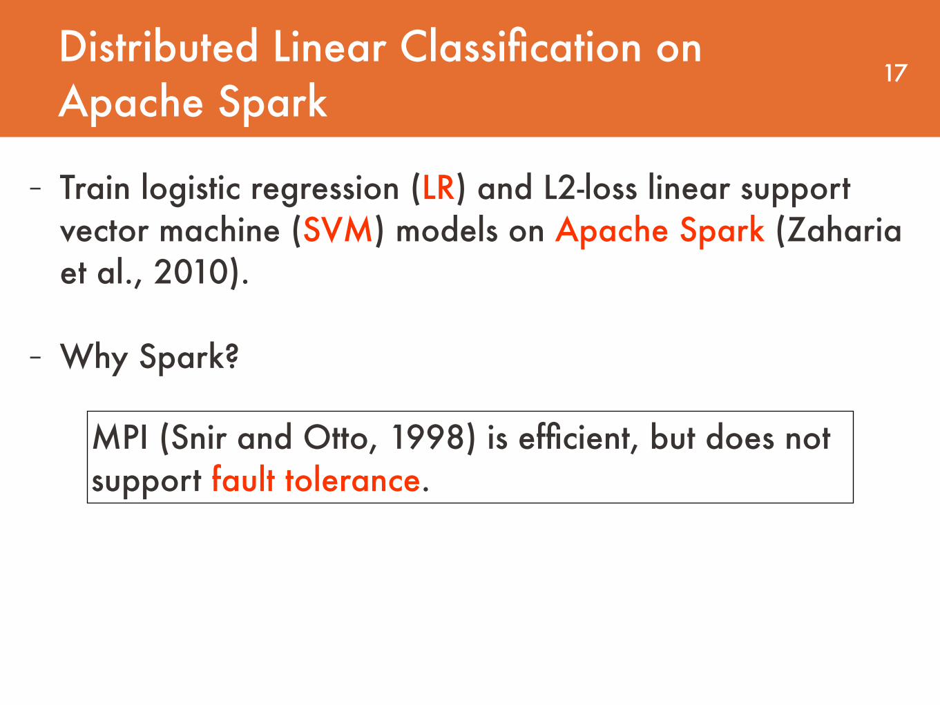
- Why Spark?



Spark combines advantages of both frameworks.


20

- Why Spark?

MPI (Snir and Otto, 1998) is e cient, but does not support fault tolerance.



Communications conducted in-memory.


21

- Why Spark?


Communications conducted in-memory.

Supports fault tolerance.

- However, Spark is new and still under development.(2014)

- Therefore it is necessary to examine important implementation issues to ensure efficiency.

Apache Spark 22

- Only the master-slave framework.

Apache Spark 23


- Data fault tolerance: Hadoop Distributed File System (Borthakur, 2008).

Apache Spark 24



- Computation fault tolerance:

Apache Spark 25



- Computation fault tolerance: Read-only Resilient Distributed Datasets (RDD) and lineage (Zaharia et al., 2012). Basic idea: reconduct operations recorded in lineage on immutable RDDs.

Apache Spark 26

- Lineage (Zaharia et al., 2012). Spark firstly creates a logical plan (namely data dependency graph) for each application.

Apache Spark 27

- Lineage (Zaharia et al., 2012). Then it transforms the logical plan into a physical plan (a DAG graph of map/reduce stages and map/reduce tasks).

Apache Spark 28

- Lineage (Zaharia et al., 2012). After that, concrete map/reduce tasks will be lanuched to process the input data.

Apache Spark (skip) 29

package org.apache.spark.examplesimport java.util.Randomimport org.apache.spark.{SparkConf, SparkContext}import org.apache.spark.SparkContext._/** * Usage: GroupByTest [numMappers] [numKVPairs] [valSize] [numReducers] */object GroupByTest { def main(args: Array[String]) { val sparkConf = new SparkConf().setAppName("GroupBy Test") var numMappers = 100 var numKVPairs = 10000 var valSize = 1000 var numReducers = 36 val sc = new SparkContext(sparkConf) val pairs1 = sc.parallelize(0 until numMappers, numMappers).flatMap { p => val ranGen = new Random var arr1 = new Array[(Int, Array[Byte])](numKVPairs) for (i <- 0 until numKVPairs) { val byteArr = new Array[Byte](valSize) ranGen.nextBytes(byteArr) arr1(i) = (ranGen.nextInt(Int.MaxValue), byteArr) } arr1 }.cache // Enforce that everything has been calculated and in cache pairs1.count println(pairs1.groupByKey(numReducers).count) sc.stop() }}

GroupByTest.scala- Lineage (Zaharia et al., 2012). spark code example

30

package org.apache.spark.examplesimport java.util.Randomimport org.apache.spark.{SparkConf, SparkContext}import org.apache.spark.SparkContext._/** * Usage: GroupByTest [numMappers] [numKVPairs] [valSize] [numReducers] */object GroupByTest { def main(args: Array[String]) { val sparkConf = new SparkConf().setAppName("GroupBy Test") var numMappers = 100 var numKVPairs = 10000 var valSize = 1000 var numReducers = 36 val sc = new SparkContext(sparkConf) val pairs1 = sc.parallelize(0 until numMappers, numMappers).flatMap { p => val ranGen = new Random var arr1 = new Array[(Int, Array[Byte])](numKVPairs) for (i <- 0 until numKVPairs) { val byteArr = new Array[Byte](valSize) ranGen.nextBytes(byteArr) arr1(i) = (ranGen.nextInt(Int.MaxValue), byteArr) } arr1 }.cache // Enforce that everything has been calculated and in cache pairs1.count println(pairs1.groupByKey(numReducers).count) sc.stop() }}

GroupByTest.scala

[1]. Initialize SparkConf. [2]. Initialize numMappers=100, numKVPairs=10,000, valSize=1000, numReducers= 36. [3]. Initialize SparkContext, which creates the necessary objects and actors for the driver. [4].Each mapper creats an arr1: Array[(Int, Byte[])], which has numKVPairs elements. Each Int is a random integer, and each byte array's size is valSize. We can estimate Size(arr1) = numKVPairs * (4 + valSize) = 10MB, so that Size(pairs1) = numMappers * Size(arr1) ＝1000MB.

[5].Each mapper is instructed to cache its arr1 array into the memory. [6].The action count() is applied to sum the number of elements in arr1 in all mappers, the result is numMappers * numKVPairs = 1,000,000. This action triggers the caching of arr1s. [7].groupByKey operation is performed on cached pairs1. The reducer number (a.k.a., partition number) is numReducers. Theoretically, if hash(key) is evenly distributed, each reducer will receive numMappers * numKVPairs / numReducer ＝

27,777 pairs of (Int, Array[Byte]), with a size of Size(pairs1) / numReducer = 27MB. [8].Reducer aggregates the records with the same Int key, the result is (Int, List(Byte[], Byte[], ..., Byte[])). [9].Finally, a count() action sums up the record number in each reducer, the final result is actually the number of distinct integers in pairs1.

- Lineage (Zaharia et al., 2012). spark code explanation

Apache Spark (skip)

Apache Spark 31

- Read-only Resilient Distributed Datasets (RDD)

RDD is a mechanism capable of holding the data to be repeatedly used in the memory.MapReduce of Hadoop had been held, fault tolerance, data locality, scalability has taken over as it is.

1.an RDD is a read-only, partitioned collection of records.

2.an RDD has enough information about how it was derived from other datasets (its lineage)

3.persistence and partitioning

4.lazy operations

Apache Spark 32

- Read-only Resilient Distributed Datasets (RDD)

reference

- Resilient Distributed Datasets: A Fault-Tolerant Abstraction for In-Memory Cluster Computinghttp://www-bcf.usc.edu/~minlanyu/teach/csci599-fall12/papers/nsdi_spark.pdf

- My article of Qiitahttp://qiita.com/Hiroki11x/items/4f5129094da4c91955bc

http://www-bcf.usc.edu/~minlanyu/teach/csci599-fall12/papers/nsdi_spark.pdf

http://qiita.com/Hiroki11x/items/4f5129094da4c91955bc

Outline 33

1. Introduction

2. Approach


4. Related Works


Logistic Regression and Linear Support Vector Machine

34

Most linear classification models consider the following optimization problem

{(xi,yi)}li=1, xi ∈ Rn, yi ∈ {−1,1}, ∀i, :Given a set of training label-instance pairs C > 0 : User-specified parameter

ξ(w;xi,yi) : loss function


35


The objective function f has two parts: the regularizer that controls the complexity of the model, and the loss that measures the error of the model on the training data. The loss function ξ(w;xi,yi) is typically a convex function in w.

regularizer loss function


36


Problem (1) is referred as L1-loss and L2-loss SVM if (2) and (3) is used, respectively.

It is known that (2) and (3) are differentiable while (2) is not and is thus more difficult to optimize. Therefore, we focus on solving LR and L2-loss SVM in the rest of the paper.


37


Problem (1) is referred as LR if (4) is used.


38


{(xi,yi)}li=1, xi ∈ Rn, yi ∈ {−1,1}, ∀i, :Given a set of training label-instance pairs C > 0 : User-specified parameter

ξ(w;xi,yi) : loss function

Use a trust region Newton method to minimize f(w) (Lin and Mor e, 1999).

Trust Region Newton Method 39

- Trust region Newton method is a type of truncated Newton approach.

- We consider the trust region method (Lin and Mor´e, 1999), which is a truncated Newton method to deal with general bound-constrained optimization problems (i.e., variables are in certain intervals).

- At each iteration of a trust region Newton method for minimizing f(w), we have an iterate wt, a size ∆t of the trust region, and a quadratic model.


To discuss Newton methods, we need the Hessian of f(w):

Truncated Newton method(skip) 40

- Trust region Newton method is a type of truncated Newton approach.

- To save time, one may use only an“approximate” Newton direction in the early stages of the outer iterations.

- Such a technique is called truncated Newton method (or inexact Newton method).

Newton Method (skip) 41

- Newton's method assumes that the function can be locally approximated as a quadratic in the region around the optimum, and uses the first and second derivatives to find the stationary point.

- In higher dimensions, Newton's method uses the gradient and the Hessian matrix of second derivatives of the function to be minimized.

To discuss Newton methods, we need the Hessian of f(w):

42

Up to this point

Trust Region Newton Method

At iteration t, given iterate wt and trust region ∆t > 0, solve

43

(6) is the second-order Taylor approximation of

Adjust the trust region size by ρt. If n is large: ∈ Rn×n is too large to store. Consider Hessian-free methods.

Trust Region Newton Method

At iteration t, given iterate wt and trust region ∆t > 0, solve

44

(6) is the second-order Taylor approximation of

Because is too large to be formed and stored, a Hessian-free approach of applying CG (Conjugate Gradient) iterations is used to approximately solve (5) .

At each CG iteration we only need to obtain the Hessian-vector product with some vector generated by the CG procedure.

Use a conjugate gradient (CG) method.

CG is an iterative method: only needs for some at each iteration.(it’s not necessary to calculate ∇2f (wt ))

For LR and SVM, at each CG iteration we compute

is the data matrix and D is a diagonal matrix with values determined by wt.

Trust Region Newton Method 45

Hessian-free methods.

- an algorithm for the numerical solution of particular systems of linear equations, namely those whose matrix is symmetric and positive-definite.

Conjugate gradient (CG) method (skip) 46

Distributed Hessian-vector Products

- (8) is bottleneck which is the product between the Hessian matrix r2f(wt) and the vector si

- This operation can possibly be parallelized in a distributed environment as parallel vector products.

47


- first partition the data matrix X and the labels Y into disjoint p parts.

- reformulate the function, the gradient and the Hessian- vector products of (1) as follows.

48


Data matrix X is distributedly stored

The functions and are the map functions operating on the k-th partition. We can observe that for computing (12)-(14), only the data partition Xk is needed in computing.

49


- p ≥ (#slave nodes) for parallelization. - Two communications per operation:

1. Master sends wt and the current v to the slaves. 2. Slaves return X T Di Xi v to master.

- The same scheme for computing function/gradient.

Data matrix X is distributedly stored

50

Outline 51

1. Introduction

2. Approach


4. Related Works


Implementation design 52

- In this section, they study implementation issues for their software.



- They name their distributed TRON implementation Spark LIBLINEAR because algorithmically it is an extension of the TRON implementation in the software LIBLINEAR[10]



- They name their distributed TRON implementation Spark LIBLINEAR because algorithmically it is an extension of the TRON implementation in the software LIBLINEAR[10]

- Spark is implemented in Scala, we use the same language. So, The implementation of Spark LIBLINEAR involves complicated design issues resulting from Java, Scala and Spark.



For example, in contrast to traditional languages like C and C++, similar expressions in Scala may easily behave differently.



For example, in contrast to traditional languages like C and C++, similar expressions in Scala may easily behave differently.

It is hence easy to introduce overheads in developing Scala programs


- They analyze the following different implementation issues for efficient computation, communication and memory usage.

•Programming language: ◦ Loop structure ◦ Data encapsulation •Operations on RDD: ◦ Using mapPartitions rather than map ◦ Caching intermediate information or not •Communication: ◦ Using broadcast variables ◦ The cost of the reduce function


- They analyze the following different implementation issues for efficient computation, communication and memory usage.

•Programming language: ◦ Loop structure ◦ Data encapsulation •Operations on RDD: ◦ Using mapPartitions rather than map ◦ Caching intermediate information or not •Communication: ◦ Using broadcast variables ◦ The cost of the reduce function

related to Java and Scala

related to Spark

60

- From (12)-(14), clearly the computational bottleneck at each node is on the products between the data matrix Xk

(or XkT ) and a vector v.

To compute this matrix-vector product, a loop to conduct inner products between all xi ∈ Xk and v is executed many times, it is the main computation in this algorithm.

Scala Issue: Loop structures

61

- From (12)-(14), clearly the computational bottleneck at each node is on the products between the data matrix Xk

(or XkT ) and a vector v.

To compute this matrix-vector product, a loop to conduct inner products between all xi ∈ Xk and v is executed many times, it is the main computation in this algorithm.

- Although a for loop is the most straightforward way to implement an inner product, unfortunately, it is known that in Scala, a for loop may be slower than a while loop.2


62

- To study this issue, we discuss three methods to implement the inner product: for-generator, for-range and while.

for-generator

for-range

while


63Experiment Data Information

density: avg. ratio of non-zero features per instance. ps : used for the experiments of loops and encapsulation pe : applied for the rest. In the experiments of loops and encapsulation

Scala Issue: Loop structures 64

- Use one node in this experiment.


- Use two nodes in this experiment.


two nodesone node

The reason is that when data is split between two nodes, each node requires conducting fewer loops.

67

- The translation comes with overheads and the combination becomes complicated when more operations are applied.

- The optimization of a for expression has not been a focus in Scala development because this expression is too imperative to consist with the functional programming principle.

- In contrast, a while loop is a loop rather than an expression.


68

- The translation comes with overheads and the combination becomes complicated when more operations are applied.

- The optimization of a for expression has not been a focus in Scala development because this expression is too imperative to consist with the functional programming principle.

- In contrast, a while loop is a loop rather than an expression.

- The while loop is chosen to implement their software.


69

- follow LIBLINEAR to represent data as a sparse matrix, where only non-zero entries are stored. This strategy is important to handle large-scale data.

Scala Issue: Encapsulation

70



For example, for a given 5-dimensional feature vector (2, 0, 0, 8, 0), only two index- value pairs of non-zero entries are stored.

71



For example, for a given 5-dimensional feature vector (2, 0, 0, 8, 0), only two index- value pairs of non-zero entries are stored.

- Investigate how to store the index-value information such as “1:2” and “4:8” in memory. The discussion is based on two encapsulation implementations: the Class approach (CA) and the Array approach (AA).

72

- CA encapsulates a pair of index and feature value into a class, and maintains an array of class objects for each instance.


73



- In contrast, AA directly uses two arrays to store indices and feature values of an instance.

74



- In contrast, AA directly uses two arrays to store indices and feature values of an instance.

- AA is faster because it directly accesses indices and values, while the CPU cache must access the pointers of class objects first if CA is applied

75

- The second term of the Hessian-vector product (7) can be represented as the following form.

RDD: Using mapPartitions rather than map

where a(yi,xi,w,v) = Di,ixTi v, can be computed by either map or mapPartitions.

76

- The second term of the Hessian-vector product (7) can be represented as the following form.



77

- Then map and reduce operations can be directly applied. - Considerable overheads occur in the map operations

because for each instance xi, an intermediate vector a(xi, yi, w, v)xi is created.


78

- In addition to the above-mentioned overheads, the reduce function in Algorithm 3 involves complicated computation.

- Then map and reduce operations can be directly applied. - Considerable overheads occur in the map operations

because for each instance xi, an intermediate vector a(xi, yi, w, v)xi is created.


79



80

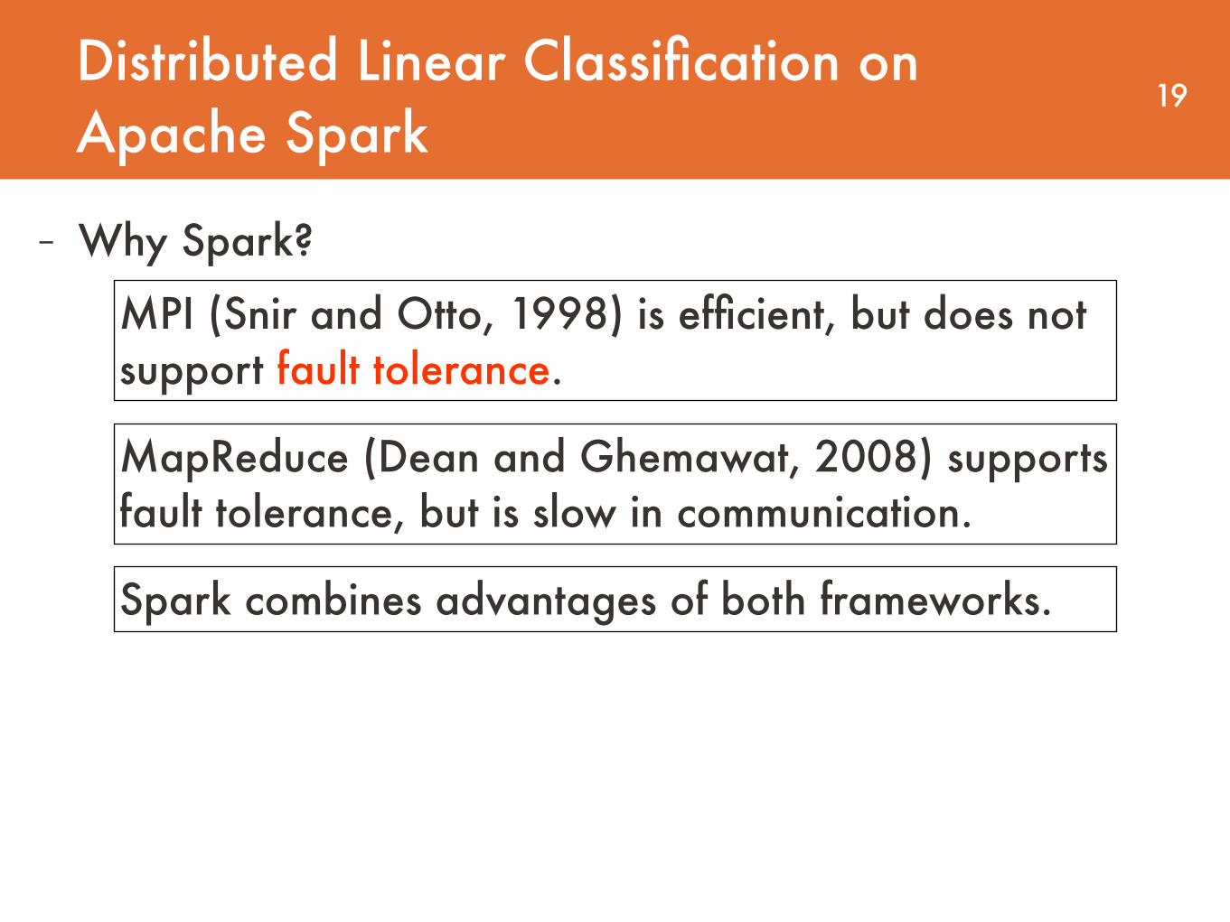
- To avoid the overheads and the complicated additions of sparse vectors, they consider the mapPartitions operation in Spark.


81

- This setting ensures that computing a Hessian-vector product involves only p intermediate vectors.

- The overheads of using map- Partitions is less than that of using map with l intermediate vectors.


82

- Note that the technique of using mapPartitions can also be applied to compute the gradient.


83RDD: Using mapPartitions rather than map

- Use 16 nodes in this experiment.

- the longer running time of map implies its higher computation cost

84

- The calculations of (12)-(14) all involve the vector (Yk Xk w).

- Instinctively, if this vector is cached and shared between different operations, the training procedure can be more efficient.

- In fact, the single-machine package LIBLINEAR uses this strategy in their implementation of TRON.

RDD: Caching intermediate information or not

85

- Spark does not allow any single operation to gather information from two different RDDs and run a user-specified function such as (12), (13) or (14).

- It is necessary to create one new RDD per iteration to store both the training data and the information to be cached.

- Unfortunately, this approach incurs severe overheads in copying the training data from the original RDD to the new one.


86

- Based on the above discussion, they decide not to cache (Yk

Xk w) because recomputing them is more cost-effective.

- This example demonstrates that specific properties of a parallel programming framework may strongly affect the implementation.


87

- In Algorithm 2, communication occurs at two places. The first one is sending w and v from the master machine to the slave machines, and the second one is reducing the results of (12)-(14) to the master machine.

RDD: Communication

88

- In Spark, when an RDD is split into partitions, one single operation on this RDD is divided into tasks working on different partitions.

- Under this setting, many redundant communications occur because just need to send a copy to each slave machine but not each partition.

- In such a case where each partition shares the same information from the master, it is recommended to use broadcast variables

RDD: Using Broadcast Variables

89

- Use broadcast variables to improve.

RDD: Using Broadcast Variables

Read-only variables shared among partitions in the same node.

Cached in the slave machines.

90RDD: The Cost of the reduce Function

- Slaves to master: Spark by default collect results from each partition separately.

- Use the coalesce function: Merge partitions on the same node before communication.


Use 16 nodes in this experiment.

Fig. 4. Broadcast variables and coalesce: We present running time (in seconds) versus the relative objective value difference. We run LR with C = 1 on 16 nodes. Note that broadcast-cl represents the implementation with both broadcast variables and the coalesce function.


- for data with few features like covtype and webspam, adopting broadcast variables slightly degrades the efficiency because the communication cost is low and broadcast variables introduce some overheads.

- Regarding the coalesce function, it is beneficial for all data sets.

Outline 93

1. Introduction

2. Approach


4. Related Works


Related Works 94

- MLlib is a machine learning library implemented in Apache Spark.

- A stochastic gradient method for LR and SVM (but default batch size is the whole data).

Related Works 95

Use 16 nodes in this experiment.

Fig. 6. Comparison with MLlib: We present running time (in seconds, log scale) versus the relative objective value difference. We run LR with C = 1 on 16 nodes.

Related Works 96

- The convergence of MLlib is rather slow in comparison with Spark LIBLINEAR.

- The reason is that the GD method is known to have slow convergence, while TRON enjoys fast quadratic local convergence for LR. Note that as MLlib requires more iterations to converge, the communication cost is also higher.

Related Works 97

- A C++/MPI implementation by Zhuang et al. (2014) of the distributed trust region Newton algorithm in this paper.

- No fault tolerance.

- Should be faster than our implementation:

More computational e cient: implemented in C++.More communicational e cient: the slave-slave structure with all-reduce only communicates once per operation.

- Should be faster, but need to know how large is the difference.

Related Works 98

m means multi-core

Related Works

m means multi-core

99

Related Works 100

m means multi-core

Related Works 101

m means multi-core

- using multiple cores is not beneficial on yahoo-japan and yahoo-korea.

- A careful profiling shows that the bottleneck of the training time on these data sets is communication and using more cores does not reduce this cost.

Outline 102

1. Introduction

2. Approach


4. Related Works


Discussions and Conclusions 103

- Consider a distributed trust region Newton algorithm on Spark for training LR and linear SVM.



- Many implementation issues are thoroughly studied with careful empirical examinations.




- Implementation in this paper on Spark is competitive with state-of-the-art packages. (2014)




- Implementation in this paper on Spark is competitive with state-of-the-art packages. (2014)

- Spark LIBLINEAR is an distributed extension of LIBLINEAR and it is available.

Large scale logistic regression and linear support vector machines using spark

Data & Analytics

Transcript of Large scale logistic regression and linear support vector machines using spark