Large N lattice gauge theory results and their interpretation · Large N lattice gauge theory...

The large N limitLattice calculation of large N observables

Conclusions

Large N lattice gauge theory resultsand their interpretation

Biagio Lucini

STRONGnet2011, ECT∗, Trento, October 2011

B. Lucini Large N lattice gauge theories


Conclusions

1 The large N limit

2 Lattice calculation of large N observablesConfinement and asymptotic freedomGlueballsMesons

3 Conclusions



Conclusions

The ’t Hooft large N limit

In QCD some phenomena (confinement, chiral symmetrybreaking) are non-perturbativeLattice calculations are successful in this regime, but moreeffective if some analytic guidance is availableIf we embed QCD in a larger context (SU(N) gauge theorywith Nf quark flavours), the theory simplify in the limitN →∞, Nf and g2N = λ fixed. Yet, it is non-trivial.Perhaps QCD is physically close to this limit?However large N QCD is still complicated enough that ananalytic solution has not been foundLattice calculations can shed light on the existence of thelimiting theory and on the proximity of QCD to it



Conclusions

String-gauge dualities

There are several examples of dualities between gaugetheories on the boundary of a manifold and string theoriesin the bulk of the same manifoldCalculations in the string theory side are often onlypossible in the supergravity limit of the string theory, whichcorresponds to the large N limit of the gauge theoryLattice calculations can assess the relevance of thosetechniques for real world QCD



Conclusions

SU(N) Gauge Theory with fermionic matter

L = − 12g2 TrGµν(x)Gµν(x) +

Nf∑i=1

ψi(x) (iγµ (∂µ + iAµ))−mi)ψi(x)

with Aµ(x) =∑

a Aaµ(x)ta, ta generators of SU(N) and

Gµν(x) = ∂µAν(x)− ∂νAµ(x) + [Aµ(x),Aν(x)]

Invariance under gauge transformations Λ ∈ SU(N)

Aµ(x) → ΛAµ(x)Λ†(x)− i (∂µΛ(x)) Λ†(x) , ψi(x) → Λ(x)ψi(x)

QCD is a SU(3) Gauge Theory with 6 fermion flavours



Conclusions

Non-perturbative properties of QCD

Confinement: asymptotic states are colorless bound statesof quarks and gluonsChiral symmetry breaking: a mass for the quarks isdynamically generated

These properties are common to all SU(N) Gauge Theorieswith Nf flavours (Nf < (11/2)N)



Conclusions

The ’t Hooft large N limit

SU(N) gauge theory (possibly enlarged with Nf fermions in thefundamental representation)

= f (g2N)

A sensible, non-trivial large N limit can be defined by keepingfixed λ = g2N, with Nf fixed (’t Hooft)



Conclusions

Planar graphs

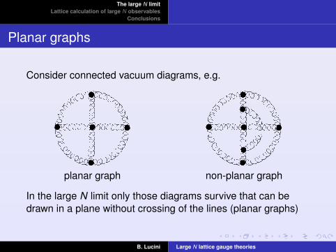
Consider connected vacuum diagrams, e.g.

planar graph non-planar graph

In the large N limit only those diagrams survive that can bedrawn in a plane without crossing of the lines (planar graphs)



Conclusions

Double line representation

Regarding the flow of the colour indices a gluon propagator isequivalent to a quark and an antiquark propagators



Conclusions

Diagrammatic at large N

For each vertex: NFor each propagator: 1/NFor each loop: N

⇒ 〈〉 ∝ NF−E+V

Euler characteristic χ = F − E + V = 2− 2H − B1 The leading connected vacuum-to-vacuum graphs are of

order N2 (planar graphs made of gluons only)2 The leading connected vacuum-to-vacuum graphs with

quark lines are of order N (planar graphs with just onequark loop at the boundary)

3 Corrections down by factors of 1/N2 in the gauge theoryand by factors of 1/N in the theory with fermions



Conclusions

Phenomenology and large N

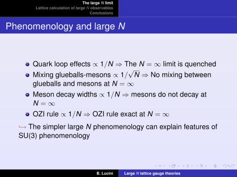
Quark loop effects ∝ 1/N ⇒ The N = ∞ limit is quenchedMixing glueballs-mesons ∝ 1/

√N ⇒ No mixing between

glueballs and mesons at N = ∞Meson decay widths ∝ 1/N ⇒ mesons do not decay atN = ∞OZI rule ∝ 1/N ⇒ OZI rule exact at N = ∞

↪→ The simpler large N phenomenology can explain features ofSU(3) phenomenology



Conclusions

Confinement and asymptotic freedomGlueballsMesons

Large N limit on the lattice

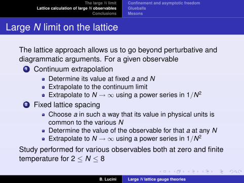
The lattice approach allows us to go beyond perturbative anddiagrammatic arguments. For a given observable

1 Continuum extrapolationDetermine its value at fixed a and NExtrapolate to the continuum limitExtrapolate to N →∞ using a power series in 1/N2

2 Fixed lattice spacingChoose a in such a way that its value in physical units iscommon to the various NDetermine the value of the observable for that a at any NExtrapolate to N →∞ using a power series in 1/N2

Study performed for various observables both at zero and finitetemperature for 2 ≤ N ≤ 8



Conclusions


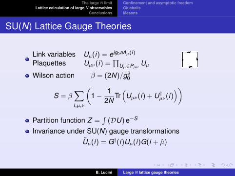
SU(N) Lattice Gauge Theories

Link variables Uµ(i) = eig0aAµ(i)

Plaquettes Uµν(i) =∏

Uµ∈PµνUµ

Wilson action β = (2N)/g20

S = β∑i,µ,ν

(1− 1

2NTr(

Uµν(i) + U†µν(i)

))

Partition function Z =∫

(DU) e−S

Invariance under SU(N) gauge transformationsUµ(i) = G†(i)Uµ(i)G(i + µ)



Conclusions


Bulk phase transition ⇒ avoided if β is large enough’t Hooft’s coupling

λ = g20N ⇒ β(N)

β(N ′)=

N2

N ′2

Tadpole improvement

g2I =

g20

〈UP〉⇒ βI(N)

βI(N ′)=

N2

N ′2



Conclusions


Correlation matrix

Trial operators Φ1(t), . . . ,Φn(t) with the quantum numbers ofthe state of interest

Cij(t) = 〈0| (Φi(0))† Φj(t)|0〉= 〈0| (Φi(0))† e−HtΦj(0)eHt |0〉

=∑

n

〈0| (Φi(0))† |n〉〈n|e−HtΦj(0)eHt |0〉

=∑

n

e−∆Ent〈0| (Φi(0))† |n〉〈n|Φj(0)|0〉

=∑

n

c∗incjne−∆Ent = δij

∑n

|cin|2e−amnt →t→∞

δij |ci1|2e−am1t



Conclusions


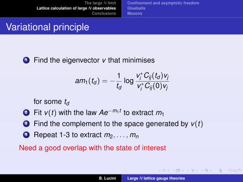
Variational principle

1 Find the eigenvector v that minimises

am1(td) = − 1td

logv∗i Cij(td)vj

v∗i Cij(0)vj

for some td2 Fit v(t) with the law Ae−m1t to extract m1

3 Find the complement to the space generated by v(t)4 Repeat 1-3 to extract m2, . . . ,mn

Need a good overlap with the state of interest



Conclusions


String tension

Confining potential: V = σR

Polyakov loop Pk (i) = 1N Tr

∏Lj=0 Uk (i + j k)

P(t) =∑~n,k

Pk (~n, t)

C(t) = 〈(P(0))† P(t)〉 =∑

j

|cj |2e−amj t →t→∞

|cl |2e−aml t

aml ' a2σL− π(D − 2)

6L



Conclusions


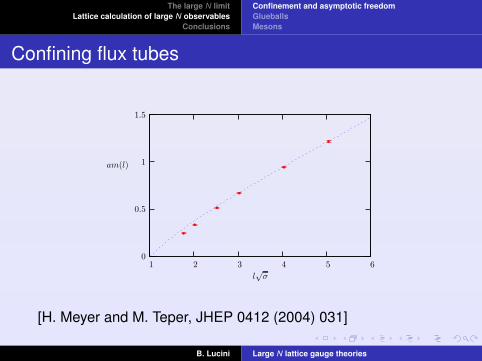
Confining flux tubes14 MTeper printed on December 17, 2009

l!

!

am(l)

654321

1.5

1

0.5

0

Fig. 5. Ground state energy of a flux loop winding around a spatial torus of lengthl, in SU(6) and D = 3 + 1.

apparent from the plot that we do indeed have the (approximately) linearincrease with l that indicates linear confinement. So that you can judgewhat is the length l in physical units, I have used the value of a

!! from

our fits to translate the lattice size l = aL into physical units using l!

! =aL!

! = L" a!

!. Since we expect the intrinsic width of a flux tube to beO(1/

!!) we can see that our largest values of l are indeed large compared

to the flux tube width and it is reasonable to infer that what we are seeingis the onset of an asymptotic linear behaviour.

The dashed line shown on the plot represents a linear piece modified bythe Luscher correction term

m(l) = !l # "

3l. (20)

This O(1/l) correction is universal and the value used here corresponds tothe universality class of a simple bosonic string where the only masslessmodes are those of the transverse oscillations. We can see from Fig. 5 thatthis correction captures the bulk of the observed deviation from linearity.(One of course expects further corrections that are higher powers of 1/l.)So we have good evidence not only that linear confinement persists at largeN , but that it remains in the same universality class as has been establishedby previous work for SU(2) and SU(3).

[H. Meyer and M. Teper, JHEP 0412 (2004) 031]



Conclusions


Universality of the cut-off effects

[B. Lucini and M. Teper, JHEP 01106 (2001) 050]



Conclusions


The running coupling in SU(4) gauge theoryRunning coupling in pure SU(4) Yang-Mills theory Gregory Moraitis

1 10E/GeV

2

4

6

8

10

g2N

SU(2)SU(3)SU(4)

Figure 3: Running of the t’Hooft coupling g2N for N = 2,3,4.

running coupling from 7GeV down to the scale of√

σ , effectively linking the perturbative to thenon-perturbative regime. The result is similar to the previous SU(2) and SU(3) calculations alreadyperformed in that the data is well approximated by perturbation theory down to energies of the orderof the string tension. Of course, this should not be taken to mean that perturbation theory correctlyaccounts for all phenomena down to this energy, as the coupling defined through the Schrödingerfunctional may simply be an exceptional case.

Similarly, the t’Hooft coupling g2N is seen to be a universal function of E, only weakly de-pendent on N even down to N = 2, and we have extracted the N dependence of ΛSF to leadingorder in 1/N2. The large-N expectation of universality thus holds true down to energies of order√

σ , though we are unable to make any certain claims as to whether universality really extends tothe non-perturbative level, since perturbation theory itself proved adequate in the ranges of energystudied.

References

[1] M. Lüscher, R. Sommer, U. Wolff and P. Weisz, Nucl. Phys. B 389 (1993) 247 [arXiv:hep-lat/9207010].

[2] M. Lüscher, R. Sommer, P. Weisz and U. Wolff, Nucl. Phys. B 413 (1994) 481 [arXiv:hep-lat/9309005].

[3] M. Lüscher, R. Narayanan, P. Weisz and U. Wolff, Nucl. Phys. B 384 (1992) 168[arXiv:hep-lat/9207009].

[4] M. Lüscher, P. Weisz and U. Wolff, Nucl. Phys. B 359 (1991) 221.

[5] B. Lucini, M. Teper and U. Wenger, JHEP 0406 (2004) 012 [arXiv:hep-lat/0404008].

[6] B. Lucini, M. Teper and U. Wenger, JHEP 0502 (2005) 033 [arXiv:hep-lat/0502003].

[7] B. Lucini and M. Teper, JHEP 0106 (2001) 050 [arXiv:hep-lat/0103027].

7

[B. Lucini and G. Moraitis, PoSLAT2007:058 (2007)]



Conclusions


The running of the improved bare coupling22 MTeper printed on December 17, 2009

µ = 1a!

!

g2I (µ)N

121086420

6.5

5.5

4.5

3.5

Fig. 9. The running of the (improved) lattice ’t Hooft coupling for various N , fromSU(2) (green open circles) to SU(8) (red solid points).

[29] which I display in Fig. 10. For comparison I show in Fig. 11 a quiterecent compilation of experimental determinations of the running couplingthat I have borrowed from [30]. As you can see, the lattice calculation(which includes an extrapolation to the continuum limit) is more accuratethan the experimental one, and extends over a range of scales that is atleast as large. We see a very impressive comparison with 3-loop continuumrunning, beginning at very high energies where we can have confidence inthe applicability of perturbation theory.

However my purpose here is not to dwell upon these calculations in anydetail, but to point out that there have recently [31] been calculations of thiskind in SU(4). I show the corresponding plot, borrowed from [31], in Fig. 12.The range of energies is less impressive but is still non-trivial. Extractingthe ! parameter from the fits, and converting to the standard MS scheme,and using the results of earlier calculations for N = 2 and N = 3, one finds[31]

!MS!!

= 0.528(40) +0.18(36)

N2: N " 3 (31)

Since this is a straight-line fit to just 2 points, N = 3 and N = 4, it willrequire further confirmation, but it is reassuring that it is consistent withthe result in eqn(30), obtained from the quite di"erent approach of fitting

[C. Allton, M. Teper and A. Trivini, JHEP 0807 (2007) 021]



Conclusions


The Λ parameter

0 0.05 0.1 0.15 0.2 0.25

1/N20

0.2

0.4

0.6

0.8

1

!MS/"

1/2

Figure 4: The ratio !MS/!

! determined in this work as a function of 1/N2. The continuousline is the extrapolation to N = " from Ref. [22], while the dot-dashed lines delimit theregion at one sigma of confidence level (only the statistical errors are shown).

computed with two independent methods shows that at large N the systematic shouldbe under control in both cases.

5 Systematic errors

As we have seen in the previous section, albeit with larger errors, our results agreewith those reported in [22]. In order to better assess the scope of our findings, in thissection we shall discuss in detail the systematic errors of our calculation.

The main sources of systematic errors are the following:

1. Extrapolation of LMAX!

! to a = 0. We have already mentioned that this is thebiggest source of error in determining the !-parameter. In order to extrapolateLMAX

!! to a = 0, the string tension is measured for a number of lattice spacings

and then the a # 0 limit is taken according to Eq. (20). The di"culty is thelargeness of both coe"cients c1 and c2. We also have no information about therest of the series. By changing the extremes of the fitting interval and compar-ing with fits including also cubic terms (where there are su"cient values of thestring tension), we can measure the spread of those results to obtain a handle onthe systematic error connected with the extrapolation. These rather large sys-

12

[B. Lucini and G. Moraitis, Phys. Lett. B668 (2008) 226]



Conclusions


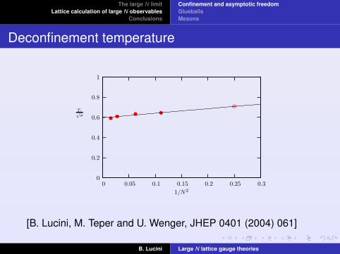
Deconfinement temperature

28 MTeper printed on December 17, 2009

such relation – but, on the other hand, this opens the door to AdS/CFTcalculations.

In Fig. 14 I show lattice calculations of Tc in units of the string tensionfor N ! [2, 8] in D = 3 + 1. All the values shown are after extrapolation tothe continuum limit [22]. If we fit with an O(1/N2) correction we obtain

Tc"!

N!2= 0.597(4) +

0.45(3)

N2: D = 3 + 1 (33)

which thus provides a prediction #N . It is perhaps surprising that this sim-ple analytic form should fit all the way down to N = 2 where the transitionhas changed from first to second order. Especially so, given that the errorsfor SU(2) and SU(3) are very small, about 0.5%. We also note that thecoe!cient of the correction is O(1) in natural units.

1/N2

Tc"!

0.30.250.20.150.10.050

1

0.8

0.6

0.4

0.2

0

Fig. 14. Deconfining temperature in units of the string tension, for continuumSU(N) gauge theories in D = 3 + 1; with O(1/N2) extrapolation to N = $.

It is interesting to see what happens in D = 2 + 1. The correspondingresults for Tc [34] are shown in Fig. 15. Now both N = 2 and N = 3 aresecond order, but a fit with just the leading correction still works for all N ,giving

Tc"!

N!2= 0.903(3) +

0.88(5)

N2: D = 2 + 1 (34)

[B. Lucini, M. Teper and U. Wenger, JHEP 0401 (2004) 061]



Conclusions


Glueball masses

[B. Lucini, M. Teper and U. Wenger, JHEP 0406 (2004) 012]



Conclusions


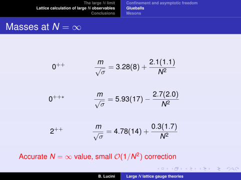
Masses at N = ∞

0++ m√σ

= 3.28(8) +2.1(1.1)

N2

0++∗ m√σ

= 5.93(17)− 2.7(2.0)

N2

2++ m√σ

= 4.78(14) +0.3(1.7)

N2

Accurate N = ∞ value, small O(1/N2) correction



Conclusions


0++ excitations

0 0.05 0.11/N2

0

0.5

1

1.5

2

2.5

am

A1++

A1++*

A1++**

Figure 10: Extrapolation to N !" of the states in the A++1 channel.

0 0.05 0.11/N2

0

0.5

1

1.5

2

2.5

am

A1-+

Figure 11: Extrapolation to N !" of the states in the A!+1 channel. We denote the less reliable states

with open symbols.

– 31 –

Lattice spacing fixed by requiring aTc = 1/6



Conclusions


Spectrum at aTc = 1/6

0

0.5

1

1.5

2

2.5

3am

Ground StatesExcitations[Lucini,Teper,Wenger 2004]

A1++ A1

-+ A2+- E++ E+- E-+ T1

+- T1-+ T2

++ T2--T2

-+T1++E-- T2

+-

Figure 20: The spectrum at N = !. The yellow boxes represent the large N extrapolation of masses

obtained in ref. [38].

0 2 4 6 8 10 12 14 16 18

!!M2

2"#

0

1

2

3

J

PC = + +PC = + -PC = - +PC = - -

Figure 21: Chew-Frautschi plot of the glueball spectrum

– 36 –

[B. Lucini, A. Rago and E. Rinaldi, JHEP 1008 (2010) 119]



Conclusions


Lattice action for full QCD

Path integral

Z =

∫(DUµ(i)) (det M(Uµ))Nf e−Sg(Uµν(i))

with

Uµ(i) = Pexp

(ig∫ i+aµ

iAµ(x)dx

)and

Uµν(i) = Uµ(i)Uν(i + µ)U†µ(i + ν)U†

ν(i)

Gauge part

Sg = β∑i,µ

(1− 1

NRe Tr(Uµν(i))

), with β = 2N/g2

0



Conclusions


Wilson fermions

Take the naive Dirac fermions and add an irrelevant term thatgoes like the Laplacian

Mαβ(ij) = (m + 4r)δijδαβ

− 12

[(r − γµ)αβ Uµ(i)δi,j+µ + (r + γµ)αβ U†

µ(j)δi,i−µ

]This formulation breaks explicitly chiral symmetry

Define the hopping parameter

κ =1

2(m + 4r)

Chiral symmetry recovered in the limit κ→ κc (κc to bedetermined numerically)



Conclusions


Quenched approximation

For an observable O

〈O〉 =

∫(DUµ(i)) (det M(Uµ))Nf f (M)e−Sg(Uµν(i))∫

(DUµ(i)) (det M(Uµ))Nf e−Sg(Uµν(i))

Assume det M(Uµ) ' 1 i.e. fermions loops are removed fromthe action

The approximation is exact in the m →∞ and N →∞ limit(g2N is fixed)↪→ the large N spectrum is quenched for m 6= 0

As N increases, unquenching effects are expected for smallerquark masses



Conclusions


Fermionic operators

Particle Bilinear JPC

σ or f0 I, ψψ 0++

π ψγ5ψ, ψγ0γ5ψ 0−+

ρ ψγiψ, ψγ0γiψ 1−−

a1 ψγ5γiψ 1++

b1 ψγiγjψ 1+−

Focus on π (0−+) and ρ (1−−)



Conclusions


Fixing the bare parameter

β fixed by imposing that aTc = 1/5

Another measured quantity (e.g. σ) could be used ⇒differences are O(1/N2)

Bare quark mass fixed (a posteriori!) by κ

StrategyStudy masses at fixed lattice spacing and various κ and fit tothe expected behaviour to compare various N



Conclusions


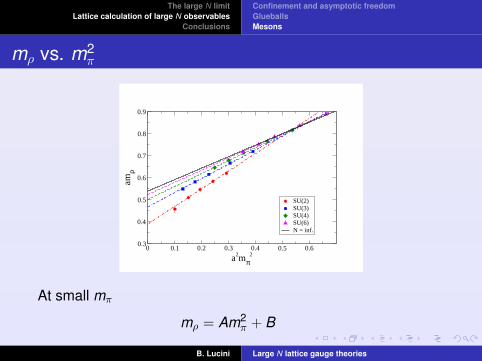
mρ vs. m2π

0 0.1 0.2 0.3 0.4 0.5 0.6a2mπ

2

0.3

0.4

0.5

0.6

0.7

0.8

0.9

amρ

SU(2)SU(3)SU(4)SU(6)N = inf.

At small mπ

mρ = Am2π + B



Conclusions


A vs. 1/N2

0.5

0.55

0.6

0.65

0.7

0.75

0.8

0.85

0 0.05 0.1 0.15 0.2 0.25

Ang. Coeff.

1/N2

Fit with an O(1/N2) correction only



Conclusions


B vs. 1/N2

0.36

0.38

0.4

0.42

0.44

0.46

0.48

0.5

0.52

0.54

0.56

0 0.05 0.1 0.15 0.2 0.25

Intercept

1/N2

Fit with an O(1/N2) correction only



Conclusions


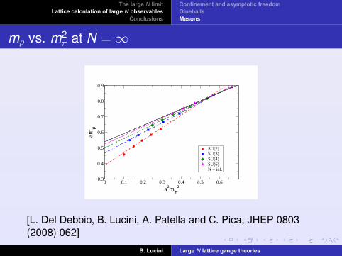
mρ vs. m2π at N = ∞

0 0.1 0.2 0.3 0.4 0.5 0.6a2mπ

2

0.3

0.4

0.5

0.6

0.7

0.8

0.9am

ρ

SU(2)SU(3)SU(4)SU(6)N = inf.

[L. Del Debbio, B. Lucini, A. Patella and C. Pica, JHEP 0803(2008) 062]



Conclusions


Chiral extrapolation of mπ - fixing σ

statistical errors. So for the ! we simply use the results from our largest volumes. Simi-

larly, at larger masses it is not necessary to include finite-volume e!ects since they will be

smaller than our statistical errors, for both the " and the !.

We note that our chiral extrapolations, described below, are not very sensitive to the

details of our finite-volume corrections. This is because the chiral fits are mostly controlled

by the data at higher mass values, which have significantly smaller errors, and are much

less sensitive to potential finite-volume corrections.

3.3 Determination of the critical hopping parameter

3.3.1 #c at finite N

0

0.1

0.2

0.3

6.3 6.4 6.5 6.6 6.7 6.8 6.9

(a m

!)2

"-1

SU(6)SU(4)SU(3)SU(2)

Figure 3: (am!)2 as a function of 1/#, eq. (3.3).

The Wilson action quark mass undergoes an additive renormalization (2a#c)!1, see

eq. (2.3). Thus we expect that the pion mass will be related to # (up to quenched chiral

logs) by,

(am!)2 = A

!

1

#!

1

#c

"

. (3.3)

By fitting to this equation we can extract #c for each N . We obtain good fits for each N ,

which we display in figure 3. Note also that the pion masses are horizontally aligned across

the di!erent N -values, indicating that we have succeeded to approximately match the #-

values to lines of constant physics, thus eliminating another possible source of systematic

bias. The values of #c that we obtain are shown in table 6. We note that while the lattice

– 8 –

[G. Bali and F. Bursa, JHEP 0809 (2008) 110]



Conclusions


mπ vs. mρ - fixing σ

table 6 to the form,

!c = !c(N =!) +c

N2. (3.5)

After including the systematic uncertainties from the chiral extrapolation we obtain values

!c(!) = 0.1596(2) and c = "0.028(3). Some of the systematics will be correlated and we

obtain a rather small "2/n # 0.27. We display the 1/N2 extrapolation of !c in figure 4. We

also include the 1/N2 extrapolation of the lattice ’t Hooft coupling at fixed string tension.

Note that this extrapolates to the value #(N =!) = 2.780(4).

3.4 The $ meson mass

3.4.1 m! at finite N

1.6

1.8

2

2.2

2.4

2.6

2.8

3

0 1 2 3 4 5 6 7

m!/"

1/2

m#2/"

SU(2)SU(3)SU(4)SU(6)

Figure 5: Fits of m!/$

% as functions of m2"/%, eq. (3.6), at di!erent N .

In chiral perturbation theory, as well as inN m!(0)/

$% B "2/n

2 1.60(5) 0.182(10) 0.2

3 1.63(4) 0.184( 9) 1.0

4 1.70(3) 0.174( 6) 0.5

6 1.64(3) 0.185( 4) 0.6

Table 7: The fit parameters of eq. (3.6)for each N , with the reduced "2-values.

the heavy quark limit, m! depends linearly on the

quark mass mq. Within our range of pion masses

m"/$

% # 1.3 . . . 2.6 we find m2" to linearly de-

pend on !!1 and therefore to be proportional to

the quark mass. Hence, we can fit our $ masses to

the parametrization,

m!$%

=m!(0)$

%+ B

m2"

%, (3.6)

– 10 –

[G. Bali and F. Bursa, JHEP 0809 (2008) 110]



Conclusions


Other topics

I deliberately did not discussStrings and k -stringsTopologyVolume reductionEguchi-KawaiThermodynamics3DOther large N limits (Veneziano, Orientifold PlanarEquivalence). . .



Conclusions

Conclusions

The lattice is a useful tool a non-perturbative investigationsof the large N limitSeveral results for various observables available by knowMany (all?) observables are well described by theexpected leading correction for 2 ≤ N ≤ 8 ⇒ SU(3) differsfrom SU(∞) by small O(1/N2) correctionsFuture work includes

Excited statesImproved meson spectrumDecay constantsEffects of fermionsOther large N generalisations (e.g. Orientifold PlanarEquivalence)


Large N lattice gauge theory results and their interpretation · Large N lattice gauge theory...

Documents

Transcript of Large N lattice gauge theory results and their interpretation · Large N lattice gauge theory...