Large Eddy Simulations on a pitching airfoil: Analysis of ...

HAL Id: hal-00375870https://hal.archives-ouvertes.fr/hal-00375870
Submitted on 16 Apr 2009
HAL is a multi-disciplinary open accessarchive for the deposit and dissemination of sci-entific research documents, whether they are pub-lished or not. The documents may come fromteaching and research institutions in France orabroad, or from public or private research centers.
L’archive ouverte pluridisciplinaire HAL, estdestinée au dépôt et à la diffusion de documentsscientifiques de niveau recherche, publiés ou non,émanant des établissements d’enseignement et derecherche français ou étrangers, des laboratoirespublics ou privés.
Large eddy simulations and stereoscopic particle imagevelocimetry measurements in a scraped heat exchanger
crystallizer geometryMarcos Rodriguez, Florent Ravelet, Rene Delfos, J. J. Derksen, Geert-Jan
Witkamp
To cite this version:Marcos Rodriguez, Florent Ravelet, Rene Delfos, J. J. Derksen, Geert-Jan Witkamp. Largeeddy simulations and stereoscopic particle image velocimetry measurements in a scraped heat ex-changer crystallizer geometry. Chemical Engineering Science, Elsevier, 2009, 64 (9), pp.2127-2135.<10.1016/j.ces.2009.01.034>. <hal-00375870>
Large Eddy Simulations and stereoscopic particle image velocimetry
measurements in a scraped heat exchanger crystall izer
M. Rodriguez Pascual 1*, F. Ravelet2, R. Delfos1, J.J. Derksen3,G.J. Witkamp1
1Process & Energy Dept. Delft University of Technology, the Netherlands
2lnstitut de Mécanique des Fluides de Toulouse, France
3 Chemical & Materials Engineering Dept., University of Alberta, Canada
*Corresponding author: [email protected]
Abstract
The transport phenomena in scraped heat exchanger crystallizers are critical for the process
performance. Fluid flow and turbulence close to the heat exchanger (HE) surface as
generated by stirring elements and scraper blades are crucial in this respect as they aim at
avoiding an insulating scale layer on the HE surface. For this reason we performed large-
eddy simulations of the turbulent flow (at a Reynolds number of 5⋅ 104) in a typical cooling
crystallizer geometry with a focus on the bottom region where the heat exchanging surface
was located. The simulations were validated with stereoscopic PIV experiments performed
higher up in the crystallizer. For reasons of optical accessibility being hindered by the
scrapers, the experiments could not be done near the heat exchanging surface. The flow
structures as revealed by the large-eddy simulations could explain the local occurrence of
scaling on an evenly cooled heat exchanger surface, and its irreproducibility caused by
instantaneous cold spots.
Keywords: Fluid Mechanics, Crystallisation, Scaling, Heat transfer, Lattice Boltzmann
Method, Scraped Heat Exchanger Crystallizers.
1. Introduction
In several types of cooling crystallization processes, solutions or melts are brought by the
action of heat exchangers into supersaturated regions where crystals will form. In industrial
continuous processes, where solution is constantly fed into the crystallizer, control and
stability of the bulk solution temperature is mandatory. For this reason a degree of
turbulence inside the crystallizer is necessary to achieve good mixing of the whole solution,
and with this aim stirrers are commonly used. Several computational and experimental
studies of fluid flow in stirred tanks have been done in the past with a view to optimizing
mixing processes motivated by their general importance in the chemical process industries
[Yianneskis et al.,(1987) ; Schäfer et al., (1998); Derksen et al., (1999) ; Derksen and Van
den Akker, (1999)]. In cooling crystallization this turbulent mixing determines the heat
transfer rates that are directly responsible for the production rates, while the residence time
in the crystallizer determines size and quality of the crystals. Particle flow interactions relate
to solid separation, attrition and agglomeration processes. Studies on the influence of the
flow on the heat and mass transfer and particle-flow interactions are of major interest but
not an easy task to perform due to the complexities related to turbulence and the wide range
of length and time-scales involved.
To bring the solution to the desired supersaturation heat exchangers (HE’s) are typically
in direct contact with the solution. The thermal boundary layer near the HE surface depends
on the crystallizer flow characteristics. Because of the higher supersaturation at the HE
surface the nucleation and growth rates of the crystals are faster than in the bulk of the
solution. This situation is responsible for the formation of a scale layer of crystals on the HE
surface in several cases of cooling crystallisation from a solution and (in particular) from a
melt, including ice crystallisation from aqueous solutions. This scale layer reduces heat
transfer, thus affecting the stability and efficiency of the crystallization process. To avoid this
scale layer formation, it is common to use mechanical actions such as scraping. Depending
on the composition of the solution and the characteristics of the mechanical scraping action
(velocity, scraper shape and applied force), a maximum temperature difference between the
solution and the heat exchanger surface can be maintained without the occurrence of
scaling. In any case, to prevent scaling the heat exchanger surface temperature also has to
be as uniform as possible, avoiding cold spots where scaling will start.
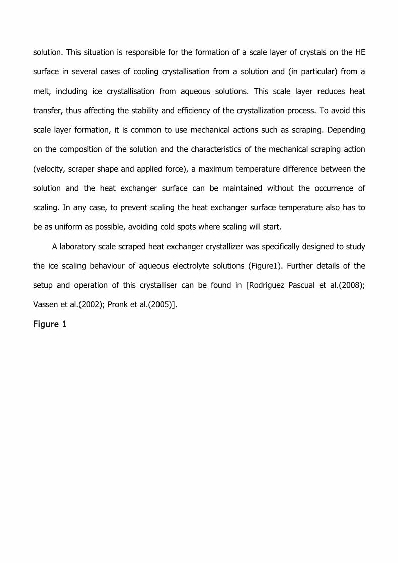
A laboratory scale scraped heat exchanger crystallizer was specifically designed to study
the ice scaling behaviour of aqueous electrolyte solutions (Figure1). Further details of the
setup and operation of this crystalliser can be found in [Rodriguez Pascual et al.(2008);
Vassen et al.(2002); Pronk et al.(2005)].
Figure 1
The location where the scaling starts as well as the lack of reproducibility and
spread in experimental results encountered in previous studies prompted us to
investigate the local temperature and heat transfer distribution across the heat
exchanger (HE) surface. These HE surface temperatures were measured by using a
thermo chromatic liquid crystal sheet (TLC) placed directly upon the HE-surface
(Figure 2). Further details of the experimental procedure are explained in Rodriguez
Pascual et al.(2008).
Figure 2
The result shows that, even though the process as such is stationary, the HE
surface temperature is far from uniform. Near the shaft and close to the wall the
heat transfer between HE and solution, reflected by the calculated heat transfer
coefficient hC(r), is lower by a factor of at least five than halfway the radius. So the
question why hC(r) varies so much over the scraped HE plate had to be answered.
Since the heating of the HE plate did not show local variations, the differences in
local heat transfer could only be caused by the flow field. The accessible part of the
flow field above the scrapers and below the stirrer was therefore investigated using
Stereoscopic Particle Image Velocimetry, (3C-PIV); further details can be found in
[Rodriguez Pascual et al.(2008)]. The axial, radial and tangential velocities of the
flow field in this middle section of the crystalliser were derived from these PIV
images.
It was, however, not feasible to measure the velocities in the lower scraper
region just above the HE surface where the actual scaling occurs because the
revolving scrapers hindered the optical accessibility required for PIV. For a more

detailed analysis of the flow field in this region we were obliged to rely on
information obtained by modelling the flow field.
To model the flow large eddy simulation (LES) in a lattice-Boltzmann scheme
for discretizing the Navier-Stokes equations was used. The major reasons for
employing a lattice Boltzmann discretization scheme are its almost full locality of
operations, its computational efficiency (in terms of floating-point operations per
lattice site and time step), and its ability to simulate flows in complex geometries. An
interface model to represent the revolving parts of the geometry was avoided by
modelling of the moving geometry with an adaptive force field technique [Derksen &
Van den Akker (1999)].
The LES methodology has proven to be a powerful tool to study and visualize
stirred tank flows, because it accounts for the unsteady and periodic behaviour of
these flows, and it can effectively be employed to explicitly resolve phenomena
directly related to the unsteady boundaries. Results of the single-phase Lattice-
Boltzmann LES code applied to stirred tank flow have been extensively compared to
phase-averaged and phase-resolved experimental data [Derksen & Van den Akker
(1999); Derksen (2001)].
The computational results of the flow field for the scraped heat exchanger
crystalliser geometry used in this study are presented in this paper. To validate the
correctness of the calculated flow field characteristics the results for the middle
section of the crystalliser were compared with the previous experimental results from
the 3C-PIV measurements.
2. Simulation setup

The Navier-Stokes equations governing the flow in the stirred tank were discretized
according to the lattice-Boltzmann method. This is an inherently parallel and efficient
numerical scheme for computational transport physics (see e.g. Succi (2001) for an
overview). The strong turbulence generated by the impeller and scrapers prohibits
direct numerical simulation: the computational effort for resolving all length and
time-scales would be too large.
In large-eddy simulations only the large-scales are resolved explicitly – the
rationale behind it is that the small scales behave more universally and are therefore
more prone to modelling than the large scales (Lesieur & Métais (1996)). Modelling
instead of resolving the small scales alleviates the computational burden. For
modelling of the small scales the standard Smagorinsky subgrid scale model was
applied. A value of cS=0.12 was adopted as the Smagorinsky constant, which is
within the range of values commonly used in shear-driven turbulence.
The stirred-scraped crystallizer configuration consists of a cylindrical, flat-
bottomed, tank with diameter of 240 mm and a height of 300 mm. The flat bottom
area of the crystallizer that acts as the heat-exchanging surface is scraped by a set
of four rotating scraper blades with a diameter of 198 mm that is driven by a vertical
shaft. Halfway the shaft a 45o pitch blade turbine with a diameter of 100 mm is
installed to keep the slurry homogeneously mixed. The geometry is defined in figure
3a. The geometry of the scraper in the simulations closely mimics the experimental
geometry (Figure 3b and 3c).
The uniform, cubic grid inherent to most of the lattice-Boltzmann formulations
comprised 1.8·107 nodes. In terms of spatial resolution: the linear size of a cubic

lattice cell amounted to approximately 1 mm. The time step in the LES was such that
one impeller revolution took 4200 time steps.
The Reynolds number that fully determines this single-phase flow is defined as
Re=ND2/ν with N the impeller speed in rps, D the diameter of the scraper (being 198
mm) and ν the kinematic viscosity of the working fluid. The continuous phase was
water with a density = 103 Kg/m3 and ν = 10-6 m2/s. The scraper and impeller were
set to rotate at a speed of 77 rpm corresponding with Re=5⋅ 104.
The LES is started from a zero velocity field. In the start-up phase of the flow
we monitor the total kinetic energy in the tank. Once this has stabilized we start
collecting flow data for later statistical analysis such as average velocity and
turbulent kinetic energy fields. .
Figure 3
3. Results and discussion
3.1. The overal l f low field in the crystall iser
The flow field as measured earlier by 3C-PIV for the middle section of the crystallizer
qualitatively explains the heat transfer distribution at the HE-surface as obtained
from the (TLC) measured surface temperatures. In the core around the shaft the
heat transfer is low because of the absence of radial and axial flow [Rodriguez
Pascual (2008)]. From about 50 mm from the shaft a secondary flow descends onto
the HE surface, and causes a much better heat transfer in the middle of the HE
surface. In contrast the local heat transfer is reduced in the outer ring of the HE
surface where the fluid temperature on its way to the wall has adapted the bottom
temperature before it ascends at the wall (Figure 4).

Figure 4
In Figure 5 the dash-dotted line represents the tangential velocity of the
scraper. The solid line representing the tangential flow measured by the PIV,
confirms that the solution is in solid body rotation up to about 40mm from the shaft.
This unwanted behaviour of the flow prevents proper mixing of the rotating solution
with the bulk, and causes low heat transfer at the bottom of this region. When
moving radially inward or outward, the flow tends to conserve its angular
momentum; in a frictionless flow this may lead to a vortex. As a simplified physical
model of the flow, we fitted the measured tangential velocity profile with the Oseen
vortex solution [Batchelor(1967)], which gradually transits from a solid-body rotation
in the inner region to a free vortex flow in the outer the region. The transition takes
place at approximately r=40mm, as shown in Figure 5. The measured tangential flow
matches qualitatively with the vortex flow in the Oseen model.
Figure 5
Although we now can roughly explain the temperature profile at the HE surface,
for a more detailed explanation the flow pattern between the scrapers just above the
surface has to be studied. Due to the problematic measuring access created by the
presence of the rotating scrapers we have for this purpose to rely on CFD
simulations. Figure 6a shows the axial and radial time averaged velocities for the
whole tank as obtained from LES computational simulations, under steady-state total
kinetic energy condition, plotted as vectors with normalized lengths. To validate the
computational results we compare the simulated flow velocities with the velocities
calculated from the 3C-PIV measurements in the same middle region of the

crystalliser. This region is indicated in Figure 6a by a black rectangle at the right
hand side of the picture.
Figure 6
Zooming in on the simulations of the flow velocities in the PIV measured area in
figure 6b demonstrates that also in the simulations axial or radial flow is nearly non
existent near the shaft. The middle area shows a strong axial flow towards the
bottom with a non existent radial contribution. Close to the outside wall the flow is
carried upwards with also no radial contribution, so these results are in good
agreement with the stereoscopic PIV data in Figure 4. The flow velocities at the three
lines across the measured area at three different heights of 45, 59 and 75 mm from
the bottom plate are presented in figure 7.
Figure 7
The tangential and axial velocities at the three heights are plotted against those
calculated from the stereoscopic PIV experiments. The results match quite well,
although the tangential and axial velocities from the PIV experiments are slightly
smaller than the LES values. Also the tangential velocities decrease when
approaching the outside wall, while the LES values increase slightly before
decreasing at the wall. The agreement is however in general very satisfactory, and
the observed differences can be explained by the unavoidable inaccuracies in the
experimental results and by the idealised computational approach.
A qualitative comparison between the PIV and LES snapshots of the same
portion of the flow (Figures 8 and 9, drawn with the same scale for the velocity
vector length) shows interesting resemblance. Clearly turbulence is much stronger
close to the outer tank wall. Furthermore the sizes of the turbulent structures
observed in PIV and LES agree quite well.
Figures 8 & 9
3.2. Flow field at the bottom part between the scrapers.
Now that we have confidence in the simulated flow data through their agreement
with the PIV results, the non accessible area just above the scraped heat exchanger
surface can be analysed from the LES simulations.
By considering time averaged flow fields resolved for the angular position of the
scraper in the LES more information about the flow patterns near the bottom can be
gained. In Figure 10 we show the average flow one in a vertical cross section
through the scrapers (Figure 10a) and one in between the scraper blades (Figure
10b).
Figure 10
The cross-section through the scrapers (Figure 10a) shows that the solution at
the tip of the scraper is forced outwards to the wall and subsequently upwards.
Another important observation is that in the middle region the downward flow above
the scraper is carried radially towards the centre of the crystalliser instead of being
carried outwards as happens in between scrapers (Figure10b).
To be able to explain the radial variation in local heat transfer, a more detailed
analysis of the region between the scrapers is needed. Figure 11 zooms in on the
time averaged flow in this area half-way between the scrapers, in the region from
the shaft to the wall on the horizontal axis and from the 3C-PIV measured area down
to the scraped HE surface on the vertical axis.

Figure 11
In the scraper region z=0 to 35 mm height from the HE surface, from the shaft
till more or less r=10 mm in the radial direction the solution has hardly an axial or
radial velocity component. Between r=10 and 15 mm a vertical down flow is
observed but with no radial component explaining the low heat transfer because
limited mixing with the rest of the tank volume. Beyond r=15 mm the liquid starts
getting axial and radial velocity components, mainly towards the outside tank wall. If
we look onto the high transfer region in Figure 11 between r=15 and 62 mm, we can
observe that this is the area where the axial velocity is positive removing the liquid
from the heat exchanger surface upwards. Here we actually have to differentiate
between two levels: the fluid trajectories starting between r=15 mm and 40 mm
from the shaft (represented by the top streamline in Figure 11) and the fluid
trajectories starting between r=40 mm and 60 mm (bottom curve in Figure11). As
we can see, the top trajectory brings the liquid higher up after which it is carried into
the main secondary flow that transports the fluid to the top of the crystalliser. In the
bottom fluid trajectory the axial velocity is lower. This keeps the liquid close to the
heat exchanger surface while approaching the outside tank wall. This makes that the
fluid in the bottom trajectory is being cooled further on its way along the trajectory.
This limits the local heat transfer coefficient. This could explain why from r=40 mm
on the TLC measurements showed that the local heat transfer coefficient starts to
decrease [Rodriguez Pascual (2008)]. Also note that fluid can get trapped by the
vortex formed at the scraper tip at the HE surface from r=100 mm until the outside
wall. This eddy retains the liquid in this region rotating without much mixing with the
rest of the liquid causing even lower local heat transfer close to the wall. Also very

close to the bottom a small inward radial flow is present in between the scrapers
(Figure 11); in Figure 10a a small radial flow is pushed outwards by the action of the
scraper. The net effect is quite important as it explains the shape of the region of
high heat transfer between two scraper passages as shown in the TLC
measurements [Rodriguez Pascual (2008)]. This region becomes less wide when the
next scraper approaches. The fluid descending from the bulk to the HE surface by
the scraper action is thus pushed outwards to the wall. Some of this fluid is captured
by the lower eddy close to the wall, and redirected to the shaft, until the next
passing scraper sends it back again to the wall. This redirected fluid is colder and
narrows the area of higher heat transfer.
Figure 12
For a better understanding, we should not forget that the three directional
components of the flow are together responsible of the complete flow field and its
influence in the local heat transfer. Figure 12 shows the time-averaged tangential,
radial and axial velocities at heights of z=5, 15 and 30 mm from the bottom in the
scraper region. Here we can see how the tangential velocity is dominating
throughout all radial positions and that the liquid is largely undergoing solid body
rotation. It is remarkable that the area where the heat transfer is relatively high
(between r=15 and 62 mm) axial and radial velocities are quite low, and we would
have missed the effect if we had not looked at the vertical cross sections. We can
however, still appreciate from figure 12 how the radial component increases from the
bottom and decreases again when approaching the top of the scraper.
So far we only considered time-averaged velocities and related flow structures
in relation to heat transfer. This is a valid approach given the relatively long response

times of the HE surface temperature. However, eventually instantaneous turbulent
flow is responsible for the local, time-dependent heat transfer. This implies that time
dependent cold spots could be formed where nucleation starts. We therefore now
turn to instantaneous realizations of the flow field as qualitative indicators for heat
transfer.
To do that we first image a horizontal cross section of the crystalliser flow at a
level halfway the height of the scrapers (Figure 13). This cross section is in the frame
of reference of the rotating scraper. It reveals that the scraper tip creates a turbulent
flow near the wall behind its blade that dissipates its energy quite rapidly (over
roughly half the distance between two scraper blades). The liquid near the tank’s
outer wall does not mix very well with the rest; it largely flows along the wall until
the next scraper blade comes by. The instantaneous differences in local turbulence
could however, provoke instantaneous cold spots. At these spots nucleation can
start, which is a statistical and instantaneous event followed by fast lateral growth.
This would explain the lack of reproducibility and spread in scaling experiments. Near
the shaft the flow is less erratic and no instantaneous cold spots are expected there.
Figure 13
The high heat transfer in the middle area of the HE surface is still difficult to
interpret from Figure 13. For this purpose vertical cross section of the flow was made
perpendicular to the scraper blade at r=60 mm from the shaft, see Figure 14.
Figure 14
This cross section shows how in the middle of a scraper blade the liquid from
the bulk is carried down to the HE surface in near the wake of the scraper. From
figure 11 we now know that this flow at the back of the scraper is pushed outwards

to the outside wall and that later on (in between the two scrapers) it is moved
upwards away from the HE surface in the region from around 15mm until 40 mm.
Therefore the contact time of the liquid with the heat exchanger surface in the
middle region of a scraper blade is lower than in the other areas, and because the
liquid comes directly from the bulk, the temperature difference compared with the
cooling liquid underneath the HE surface is higher. This down flow also reduces the
thickness of the thermal boundary layer, which enhances the heat transfer. At the
front of the scraper the liquid is pushed upwards, and most of it is moved outwards
and merges with the main secondary flow that runs to the top of the crystalliser.
Realizing that the main cause responsible for the inhomogeneous distribution of
local heat transfer on the HE surface is the axial velocity component we now consider
the instantaneous axial velocity at three horizontal cross sections at heights of 5, 15,
and 30 mm (Figure 15).
Figure 15
As we can see from Figure 15 the fluid is brought down to the heat exchanger
in the wake of the scraper blades. This downward axial velocity behind the scraper is
zero near the centre of the tank and increases (negatively) in the radial direction
until close to the tip of the scraper where it turns positive as approaching the outside
wall. As the height increases from 5 to 30 mm the downward velocity gets stronger.
This figure also shows how the down flow coming from the bulk (as we already saw
in Figure 14) is pushed up again by the front of the next scraper, and as we know
from Figure 11 also outwards to the outside wall. This means that the scraper blade’s
middle region is continuously refreshed with every scraper passage by the bulk

liquid, what explains the higher local heat transfer coefficient in the middle area of
the HE surface compared to the centre and outside areas.
4. Conclusions
Cooling crystallization often suffers from scaling that starts at specific areas on a
heat exchanger surface even if the HE surface is evenly cooled. In a previous paper
this behaviour was investigated by measuring the local temperature distribution
across a flat scraped HE surface located at the bottom of a stirred crystallizer.
These measurements showed that the temperature was not uniformly
distributed with differences larger than 4 oC. Such differences are sufficiently large to
explain local variations in scaling tendency. After excluding all other possible reasons
for this inhomogeneous distribution the fluid flow in the crystalliser seemed to be the
only responsible cause. Stereoscopic PIV measurements of the flow in the region
above the scrapers and below the stirrer were carried out, which showed that the
flow pattern in this crystallizer geometry could roughly explain the observed
inhomogeneities in heat transfer. For more detailed information on the flow pattern
between the scrapers and thus more closely to the HE surface we had to rely on
computational flow simulations, because this region was not accessible for PIV
measurements.
The flow of the total scraped HE crystalliser was therefore computationally
resolved by Large Eddy Simulations using a Lattice Boltzmann scheme. The
simulations were validated by comparison with the PIV measurements performed
previously. This provided sufficient confidence to focus on the flow pattern in the
bottom region.

Analysing the results from the LES we could explain the radial local heat
transfer coefficient distribution along the HE surface. The local heat transfer is higher
in the middle region of the HE surface between the shaft and the outer wall (from r=
15 till r= 60 mm) because the fluid comes directly from the bulk and its residence
time near the HE surface is low. The lower local heat transfer coefficient in the tank’s
centre is because the fluid is largely in solid body rotation and although (when the
scraper passes) liquid is carried up in front and down behind the scraper, it is not
mixing in the radial direction with the rest of the liquid. Beyond r=60 mm until
around r=100 mm, the local heat transfer coefficient is lower because the residence
time of the liquid close to the HE surface is higher. In between r=100 mm and the
outside wall, a worse situation for heat transfer is provoked by a static vortex that
brings the fluid into a segregated area. These fluid flow results explain the
mechanisms that provoke the local heat transfer distribution measured by the TLC
experiments. Instantaneous fluctuations in the flow are too fast to have any impact
on the temperature profile at the HE surface that depends on the different residence
times of the fluid in the different areas.
The formation of an ice layer begins in the colder areas around the centre and
near the outside wall of the HE surface, and spreads along the HE surface. In a clear
fluid, scale formation starts by primary heterogeneous nucleation at the HE surface
followed by a fast lateral growth rate. This nucleation is a statistical event, where
local time-dependent cooling conditions play a role. Because the subsequent lateral
growth is very fast, irreproducibility can be expected. Under crystallizing conditions
crystals may also land on the HE surface. These crystals may firmly attach to the
surface by growth, before they are removed by the scraper and contribute to the

scale formation. This process also depends upon accidental events that make
altogether the appearance of the ice scaling layer time dependent and difficult to
predict.
The importance of the flow field for controlling the scale layer formation on the
HE surface during crystallisation has been demonstrated. In the context of fluid flow,
unexpected results found previously [Vaessen et al.(2002)]; Pronk et al.(2005)]
where for example lower stirring/scraping velocities show less scaling formation may
be understandable. Further computational analysis in this sense including solving of
the local heat transfer and liquid temperature then has to be done.
Large eddy simulations using a lattice Boltzmann scheme have proven to be a
powerful tool to investigate the flow in future complicated crystallizer designs with
various scraper geometries, since inhomogeneities in heat transfer impose strong
limitations on the performance of the process.
5. Outlook
The simulations presented here are those of the fluid dynamics of a clear liquid.
Under crystallising conditions however, even without the occurrence of scaling,
crystals that are developed in the bulk of the fluid may come close to or even land on
the heat exchanger surface. These crystals are transported back into the bulk liquid
by the flow induced by the revolving scrapers. In addition, under scaling conditions
mostly small particles are scraped off the scale layer and lifted by the flow. The
scraper design has a remarkable importance here and should be such that the
particles are transported away from the HE surface by the flow; they should not
directly return to the surface by e.g. a trailing vortex. The particles are subjected to
collisions with the hardware such as the scrapers and the wall, and to particle-
particle collisions. They may even agglomerate into lumps of separate or inter-grown
particles. To properly simulate a flow which contains particles, first the particle-
particle interactions have to be included. As a second more complicated step a
coupled particle-flow interaction has to be implemented, because in areas of high
particle densities these particles will affect the flow behaviour.
In a forthcoming paper a first step in this direction has been made by
implementing the particle-particle interactions. Direct Numerical Simulations based
on a Lattice Boltzmann scheme were carried out, and the results will be compared
with an experimental visualisation of particles that are added to the fluid and that are
transported by the scraper actions.
Acknowledgment
The authors would like to thank Prof. G. M. Van Rosmalen for in-depth discussions.
6. References
Batchelor, G.K.(1967) An Introduction to Fluid Dynamics. Cambridge University
Derksen, J. J.(1999), and H. E. A. Van den Akker. Large Eddy Simulations on the
Flow Driven by a Rushton Turbine. AIChE J., 45(2),209.
Derksen, J.J., S. Doelman, and H.E.A. Van der Akker,(1999). Three dimensional LDA
measurements in the impeller region of a turbulently stirred tank. Exp.Fluids,27,522.

Derksen, J.J.(2001).Assessment of Large Eddy Simulations for Agitated Flows. Trans.
IChemE, 79A, 824.
Lesieur, M., and O. Métais.(1996).New trends in large-eddy simulations of
turbulence. Annu. Rev. Fluid Mech., 28, 45.
Pronk, P., Infante-Ferreira, C.A., Rodriguez Pascual, M. and Witkamp, G.J. (2005)
Maximum Temperature difference without ice scaling in a scraped heat exchanger
crystalliser.Proc. 16th Int. Symp. on Industrial Crystallization. pp. 1141-46
Rodriguez Pascual, M., Ravelet, F., Delfos, R., Witkamp, G.J.,(2008) Measurement of
flow field and temperature distribution in a scraped heat exchanger crystallizer,
Eurotherm, Eindhoven, May 18-22; also an extended version was submitted for
publication in International Journal of Heat and Mass Transfer .
Schäfer, M, M.Yianneskis, P. Wächter, and F. Durst.(1998).Trailing vortices around a
45o Pitched blade impeller. AICHE J.,44,1233.
Succi, S..(2001). The lattice Boltzmann equation for fluid dynamics and beyond,
Clarondon Press, Oxford.
Vaessen, R.J.C., Himawan, C. and Witkamp, G.J. (2002), Scale formation of ice from
electrolyte solutions on a scraped surface heat exchanger plate. Journal of Crystal
Growth, 237-239 (Pt.3), pp. 2172-77

Yianneskis, M.,Z. Popiolek, and J.H. Whitelaw(1987). An experimental study of the
steady and unsteady flow characteristics of stirred reactors. J.Fluid Mech.,175,537.

Figure1. Laboratory scale scraped cooling crystallizer. [Vassen et al.(2002)]

Figure 3a). Side view of the crystalliser. b). Top view of the crystalliser. c). Sideway
view of the real scraper geometry.
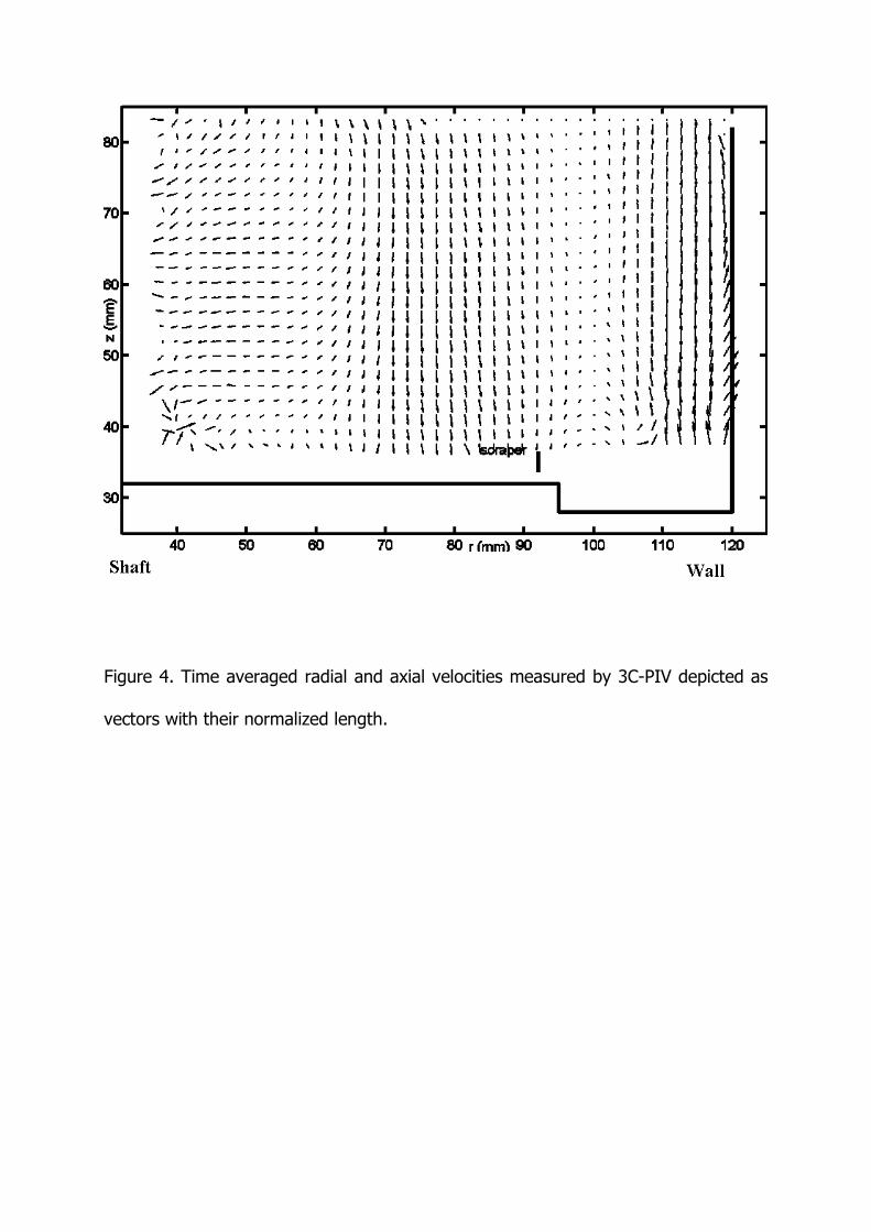
Figure 4. Time averaged radial and axial velocities measured by 3C-PIV depicted as
vectors with their normalized length.

Figure 5. Measured time-axial averaged tangential velocity of the PIV area, the
scraper velocity and the tangential velocity calculated from the Oseen approximation.

Figure 6. a) Time averaged velocity vectors of the flow field inside the scraped heat
exchanger crystalliser. The black rectangle corresponds to the area measured by 3C-
PIV. b) Computational results of the 3C- PIV measured area. The three lines across
the measured area are drawn at heights of 45, 59 and 75 mm from the bottom plate.
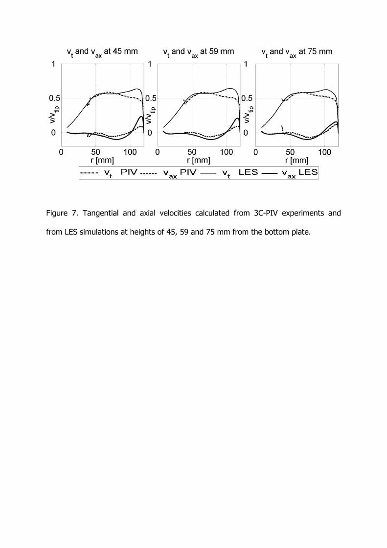
Figure 7. Tangential and axial velocities calculated from 3C-PIV experiments and
from LES simulations at heights of 45, 59 and 75 mm from the bottom plate.

Figure 8 a). Instantaneous capture of the flow from the 3C-PIV measurements.
Vectors represent the axial and radial velocity and their normalized length.b).
Instantaneous capture of the flow from the LES simulations

a) b)
Figure 10. a) Time averaged flow field of the vertical cross section through the
scrapers with an enlargement of the scraper area underneath. b) Time averaged flow
field between the scrapers with an enlargement of the scraper area underneath.
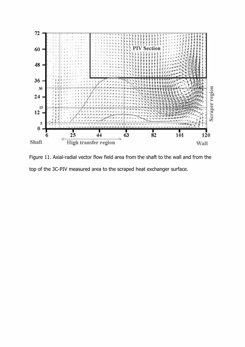
Figure 11. Axial-radial vector flow field area from the shaft to the wall and from the
top of the 3C-PIV measured area to the scraped heat exchanger surface.
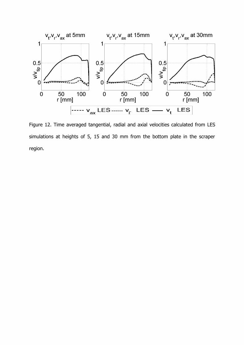
Figure 12. Time averaged tangential, radial and axial velocities calculated from LES
simulations at heights of 5, 15 and 30 mm from the bottom plate in the scraper
region.
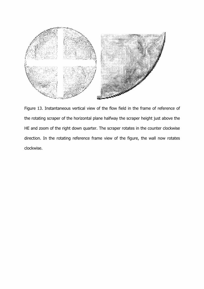
Figure 13. Instantaneous vertical view of the flow field in the frame of reference of
the rotating scraper of the horizontal plane halfway the scraper height just above the
HE and zoom of the right down quarter. The scraper rotates in the counter clockwise
direction. In the rotating reference frame view of the figure, the wall now rotates
clockwise.

Figure 14. Instantaneous flow velocities of the vertical cut of the scraper region at
the middle section of the scraper.

Figure 15. 3D surfaces of the instantaneous axial velocity at 5, 15 and 30 mm from
the heat exchanger surface.