Large Eddy Simulation of Wing Tip Vortex in the Near Field · Department of Mathematics, University...

http://www.uta.edu/math/preprint/

Technical Report 2007-13

Large Eddy Simulation of Wing Tip Vortex in the Near Field

Li JiangJiangang CaiChaoqun Liu

Large Eddy Simulation of Wing Tip Vortex in the Near Field

Li Jiang Jiangang Cai Chaoqun Liu

Department of Mathematics, University of Texas at Arlington, Arlington, Texas

September 2007

Abstract

Large eddy simulation with filtered-structure-function subgrid model and implicit large eddy

simulation (ILES without explicit subgrid model) using high-order accuracy and high resolution

compact scheme have been performed on the tip vortex shedding from a rectangular half-wing

with a NACA 0012 airfoil section and a rounded wing tip. The formation of the tip vortex and its

initial development in the boundary layer and the near field wake are investigated and analyzed

in detail. The physics, why the tip vortex, which is originally turbulent in the boundary layer, is

re-laminarized and becomes stable and laminar rapidly after shedding in the near field, is

revealed by this simulation. The computation also shows the widely used second order subgrid

model is not consistent to six-order compact scheme and would degenerate the six-order LES

results to second order. Therefore, high order schemes, gird refinement and six order subgrid

models are critical to LES approaches.

1. Introduction

Tip vortices are generated at the tip of lifting surfaces where fluid flows from the high-pressure

side to the low-pressure side. Tip vortices have significant effects on many practical engineering

problems. Wing tip vortices can result in a decrease in lift and an increase in drag. Trailing

vortices generated at the wing tip can affect the landing separation distances for aircraft. The

propeller tip-vortex cavitation on a submerged submarine can cause the serious noise problem.

The blade/vortex interaction on helicopter blades can impact the blades performances and cause

undesirable noise and vibration. The study of tip vortices is not only of great engineering

importance but also of great scientific interest and challenge. Tip vortex flow is a very

complicated flow. The tip vortex system originated from the complex three-dimensional

separated flow is highly unsteady and turbulent. The interactions between the primary and the

secondary vortices, the vortices and the separated shear layer, and that between the system of

vortices and the wakes occur simultaneously in the flow field.

Many experimental and numerical investigations of tip vortex dynamics have been conducted in

the past decades. Since noise radiation from flap side edges is known to be a major component

of non-propulsive, i.e., airframe-generated noise, a lot of efforts have been made under NASA’s

Advanced Subsonic Technology Program (Macaraeg, 1998). Khorrami (Khorrami et al, 1999)

analyzed five possible sources which cause the flow unsteadiness and then serious noises: 1)

large-scale flow fluctuation supported by the free-shear layer emanating from the flap bottom

edge and spanning the entire flap chord, 2) large-scale flow fluctuations supported by the post-

merged vortex downstream of the mid-chord region, 3) convection of a turbulent boundary layer

over the sharp edges at the flap side edge, giving rise to scattering and broadband sound radiation,

4) vortex merging, and 5) vortex breakdown. They believe the first two are most likely to be

responsible for the bulk of the concentrated audible noise generation. A linear analysis of the

shear layer instability has been made showing good agreement, in frequencies of the maximally

amplified disturbance, with the directional, microphone array measurements performed in the

QFF at NASA Langley Research Center. Further efforts to reduce the tip-vortex generated noise

have been made by using a side-edge fence (Sloff et al, 2002) and porous flap-tip treatment

(Chow et al, 2002). Choudhari (Choudhari et al, 2003) applied RANS code, CFL3D, with a

porous flap tip model to successfully simulate the time average improvement. The simulation

showed that flow communication via distributed leakage across the treatment surface leads to

reduced flap loading near the side edge. The reduced flap loading results in a reduced severity of

shear layer rollup adjacent to the side edge, a modified interaction between the side and top-edge

vortices, and significantly weaker (more diffuse) vortex structures over the aft-chord region. The

vortex structures are also slightly farther away from the side edge compared with the untreated

case. Finally, the breakdown of the side edge vortex at higher flap deflections can also be

eliminated by the porous treatment. However, their approach is the time averaged RANS. In

order to get a deeper understanding of the physics, LES is necessary to be used to capture the

flow details.

The physical behavior of a trailing vortex in the far filed downstream of the lifting body has

been of the primary interest. By comparison, the evolution of tip vortices within a few chord

lengths downstream of the wing trailing edge receives much less attention. In fact, the initial roll-

up of the wing tip vortex shows a more complex behavior. Better understanding of the formation,

structure, strength and the initial development of the wing tip vortices may provide the guide for

the tip vortex control. The present work is focused on the generation and the near field

development of a wing tip vortex. In the experiment conducted by Chow et al (Chow et al 1997)

on the rectangular half-wing model at a Reynolds number based on chord of 4.6x106, the flow

was found to be turbulent in the near field. However, the turbulence decayed quickly with

streamwise distance. This was considered to be the result of the stabilizing effect of the nearly

solid body rotation of the vortex-core mean flow. It was also found that the Reynolds shear

stresses are not aligned with the mean strain rate, indicating that an isotropic-eddy-viscosity-

based prediction method which is used by most RANS and subgrid model can not fully model

the turbulence in the vortex. Based on this experiment, Dacles-Mariani et al (Dacles-Mariani, et

al, 1996) conducted the numerical simulations of the wingtip vortex flow in the near field region.

The method of artificial compressibility was used to solve the three-dimensional incompressible

Navier-Stokes equations. The convective and pressure terms are evaluated using fifth-order

accurate flux-difference splitting based on Roe’s method. Their results showed good agreement

with the experiment data outside of the viscous vortex core. It was also found that the Baldwin-

Barth and the Spalart-Allmaras one equation turbulence models can not accurately predict tip

vortex. An ad-hoc modification of the production term was needed. It was thought that the

underprediction of the flow quantities in the core region was caused by turbulence modeling

errors. Fleig and Arakawa (Fleig and Arakawa 2003) performed simulations of tip vortex

generated by a finite blade with NACA0012 section at Reynolds numbers of 4.06x105 and

1.2x106. Smagorinsky eddy viscosity model and up to 300 million grid points were used in the

simulations. The solver is based on the second-order Beam-Warming approach and a third-order

finite-difference upwind scheme for spatial derivatives. Complex flow features associated with

the tip vortex were compared with experimental measurements for the lower Reynolds number

cases. It was found that the tip vortex constitutes a major noise source. Youssef et al (Youssef

et al 1997) conducted the temporal large-eddy simulation to study the development of large scale

structures in the wake and their interaction with the tip vortex. A model was derived to provide

an approximate velocity field in a vertical plane immediately after the trailing edge of a

rectangular wing. This velocity field was used as the initial condition for the temporal large-

eddy simulations. A modified MacCormack scheme which is explicit second order in time and

fourth order in space for the convective terms was used to solve the compressible LES equations.

Smagorinsky model was used and the Reynolds number based on the chord length is 5.3x105. It

was found that the classical sinuous mode of 2D wakes prevails in the spiral wake connecting the

vortex core to the nominally 2D wake in the middle of the wing. The large scale structures of the

spiral wake cause the formation of undulations on the core. In the studies by Labbe and Sagaut

(Labbe and Sagaut 2003), the simulations of the evolution of the near field wake vortex behind a

A300 Airbus model in high-lift configuration was carried out by solving the three-dimensional

Navier-Stokes equations for an incompressible fluid with a second order accurate scheme in time

and space. The Reynolds number based on the chord length is 1.5x105. This simulation focused

on a portion of the wake. The inlet plane was located at one wingspan behind the trailing edge of

the wing. The inlet boundary condition was provided by experiment data. As the turbulent

motion has only negligible effects on the vertical and spanwise velocity components of wake

vortices, no turbulence model was implemented. This study numerically reproduced the unsteady

properties of the vortices and compared the different frequencies with those measured

experimentally. The results showed that the main vortex is subject to a global motion which

frequencies are in the same range as those obtained experimentally.

Near field tip vortex flow is a complex turbulent flow dominated by rotation. The flow

structures have large range of scales and both velocity and pressure have large gradients

especially in the near field at high Reynolds numbers. The flow complexity requires that the

numerical methods used to study tip vortices must have high-order accuracy and high resolution.

Compact schemes have spectral-like resolution and can achieve high-order accuracy with

compact stencils. Compact schemes have been widely used in the simulations of complex flows,

especially in the direct numerical simulations of turbulent flows. The objective of this work is to

use the LES and implicit LES with high order accuracy and high resolution to investigate the

formation and the near field evolution of a wing tip vortex at high Reynolds number. The code

used in this study is based on a sixth-order compact finite difference scheme (Lele, 1992). An

outline of the paper is as follows. A brief introduction of the governing equations and the

numerical method is given in Section 2. In Section 3, the flow configuration and computational

parameters are described. Results and discussions are presented in Sections 4. Concluding

remarks are given in Section 5.

2. Governing equations and numerical methods

The governing equations solved are the conservation form of three-dimensional compressible

Navier-Stokes equations in body-fitted coordinates. The LU-SGS implicit solver (Yoon, 1992)

scheme based on the second-order backward Euler algorithm is used for the time advancing.

Spatial derivatives are calculated using the sixth-order centered compact finite differencing

(Lele, 1992) in the interior of the domain, together with fourth-order closures at points

immediately adjacent to the boundary and third-order closures at the boundary points.

Coordinate transformation metrics are also evaluated using the same compact scheme by an

approach that satisfies the geometric conservation law numerically (Gaitonde & Visbal, 1999).

High order compact filtering (Lele, 1992) is used at regular intervals to suppress the numerical

oscillation associated with the high-order centered compact scheme. Parallel computation based

on the Message Passing Interface (MPI) is utilized to improve the performance of the code. The

parallel computation is combined with the domain decomposition method. The computational

domain is divided into n equal-sized subdomains along the ξ direction. Readers may refer to our

early work (Shan et al., 2000) for more details of the parallel algorithm. The details of the

numerical method and the numerical verification and applications of the computer code can be

found in our previous work (Jiang et al., 1999a, Shan et al, 2000, Shan et al, 2005). For the large

eddy simulations, the Filtered-Structure-Function LES model (Ducros, et al, 1996) is used.

3. Flow Configuration and Computational Parameters

The flow configuration in this simulation is based on the wing tip experiment conducted by

Chow et al (Chow, et al. 1997). The computational domain includes a rectangular half-wing

with a NACA 0012 airfoil section, a rounded wing tip and the surrounding boundaries. The wing

has an aspect ratio of 0.75. The angle of attack is 10 degrees. The upstream boundary is three

chord lengths away from the leading edge of the wing. The upper and lower boundaries are four

chord lengths from the wing surface. The outflow boundary is located at 5 chord lengths

downstream. The free-stream velocity U∞, the free-stream pressure p∞, the free-stream

temperature T∞, and the chord length of the airfoil c are selected as the reference parameters for

nondimensionalization.

The flow conditions and grid parameters are summarized in Table 1. The Reynolds number

based on the free-stream velocity and the chord length is 4.6×106. In the simulation, the free-

stream Mach number is set to 0.2. The grid layout is shown in Figure 1. Axes x , y and z are

along the chord-wise direction, the spanwise direction and the normal direction. ξ, η and ζ are

computational coordinates. The numbers of grid points in ξ, η and ζ directions are 1024, 160 and

160, respectively. The C-type grid is produced in the (x,z) plane using the elliptic grid generation

method (Spekreuse, 1995). In the spanwise direction, the grids are clustered around the wing tip.

In the wall normal direction, the grids are clustered near the wing surface. The grid sizes in wall

units shown in Table 1 are estimated based on a turbulent boundary layer flow with the same

Reynolds number. To implement the parallel computation, the computational domain is divided

evenly in ξ direction. In this simulation, 64 processors are used.

Table 1. Computational parameters

Rec Ma Nξ×Nη×Nζ ∆x+

min ∆y+

min ∆z+

min

4.6×106 0.2 1024×160×160 17.5 35 2.6

Figure 1. Grid distribution Figure 2. Distribution of overlapping grids

around the rounded wingtip

The nonreflecting boundary conditions proposed by Poinsot and Lele (Poinsot & Lele, 1992)

and further developed by Jiang et al (Jiang, et al, 1999) for curvilinear coordinates are imposed at

the upstream, far field and outflow boundaries. Due to the subsonic nature of the flow, the

uniform free-stream velocities and temperature are prescribed at the upstream boundary, while

the density is determined by the nonreflecting boundary conditions. This upstream boundary

condition is different from that used in the simulation conducted by Dacles-Mariani ( Dacles-

Mariani, et al 1996), in which the inflow velocity profiles are prescribed using experimental

values. At the outflow boundary, the perfectly nonreflecting boundary condition (Jiang, et al,

1999) is used. The no-slip and the adiabatic wall boundary conditions are used on the wing

surface. To avoid the effect of the low order boundary scheme, a special treatment is

implemented at the boundaries around the wing tip. The grid distribution around the wing tip in

y-z plane is plotted in Figure 2. The overlapping region includes five grid points in η direction.

This treatment ensures the sixth-order accuracy at the tip boundaries.

It is worth to mention that in the experiment (Chow, et al. 1997), the wing was mounted inside

the wind tunnel and the incoming flow is turbulent. In addition, a strip of roughness elements

was used to fix the transition which is caused by separations near the leading edge and ensure

that the boundary layers on the suction side were turbulent and kept attached downstream of the

strip. Due to the limitation the computer resources, we had to make following changes to the

flow conditions: 1) in the simulation, the symmetry boundary condition is used at the wing root

instead of using the solid plate wall boundary conditions; 2) The incoming flow is assumed to be

a uniform free-stream flow; 3) the wing surface is smooth and no early transition is excited. We

believe these changes could make the comparison between our ILES results and experiment

difficult, but would not prevent the ILES results from revealing the physics of the tip vortex

formation and it near filed development.

4. ILES Results and Discussions

A uniform flow field is used as the initial condition for the simulation. The non-dimensional

time step based on the frees-stream velocity and the wing chord length is 4.17×10-5

c/U∞. The

corresponding CFL number is 396. The non-dimensional time has reached 4.2 c/U∞ when the

data is taken for analysis. It takes about 2 c/U∞ for the flow field of the region of interest(1.5c

downstream from the trailing edge) to be fully developed.

4.1 Instantaneous flow field

Instantaneous data are picked at t= 3.15c/U∞ when the flow field is fully developed. Figure 3

shows the instantaneous field of the axial vorticity. Figure 3(a) is the perspective view of the iso-

surface of axial vorticity, which originates from the wing tip in the form of small vortical

structures and evolves into a smooth vortex tube in the further downstream wake. On the suction

side of the wing, the flow near the wing tip is highly three-dimensional turbulent. Small vortical

structures are clearly seen inside and around the tip vortex. Near the trailing edge, spiral wake

surrounding the tip vortex is formed as the wake is skewed and laterally stretched and curved by

the rotating velocity field associated with the vortex. In the further downstream region (about

one chord length from the trailing edge), the wing tip vortex is stabilized, where the small

vortical structures are not visible around the primary tip vortex. Figure 3(b) shows the contours

of axial vorticity in a vertical plane at y=0.72 which approximately intercepts with the tip vortex

core. The evolution of the vortical structures inside and around the tip vortex can be seen clearly

on the plane.

(a)

(b)

Figure 3. Instantaneous (t= 3.15c/U∞ ) field of axial vorticity. (a) Iso-surface of vorticity

component ωx=3; (b) Contours of vorticity component ωx in the x-z plane at y=0.72

The distributions of the y- and z- components of the vorticity are plotted in Figure 4 and Figure

5 respectively. In Figure 4(a), the iso-surfaces of positive and negative y- component vorticity

are parallel to each other in a vertical layout, and both extend along the axis of the wing tip

vortex in the wake, representing a typical spiral motion of velocity field. Similar observation can

be found in Figure 5(a), where the iso-surfaces corresponding to the positive and the negative z-

component of vorticity are parallel to each other in a horizontal layout. The evolution of the y-

and z- components of the vorticity on the vertical plane at y=0.72 is shown in Figure 4(b) and

Figure 5(b).

(a)

(b)

Figure 4. Instantaneous (t= 3.15c/U∞ )field of spanwise vorticity. (a) Iso-surface of vorticity

component ωy=±3; (b) Contours of vorticity component ωy in the x-z plane at y=0.72

(a)

(b)

Figure 5. Instantaneous (t= 3.15c/U∞ ) field of vorticity in z direction. (a) Iso-surface of

vorticity component ωz=±3; (b) Contours of vorticity component ωz in the x-z plane at y=0.72

Figure 6 shows the pressure contours and velocity vectors on the cross-sections at different

streamwise locations. At x/c=0.90, the vortex structures are highly unsteady. The shear layer

separates from the rounded wing tip and rolls up generating the primary vortex. The core area of

the primary vortex is very unstable and the outer edge of the primary vortex is not smooth. Near

the junction of the wing and the rounded tip, the secondary vortex is induced by the primary

vortex and the secondary vortex rotates in the opposite direction of the primary vortex, while the

vorticity of small vortices shedding from wing tip shear layer has the same sign as the primary

vortex. At x/c=0.995, on the cross-section that is very close to the trailing edge, the center of the

primary vortex moves upward away from the surface of the wing and the size of vortex core

grows.

The secondary vortex also grows as it rolls up and merges into the primary vortex and brings

unsteadiness and instability into the core of the primary vortex. The interaction between the

primary and the secondary vortices is quite intensive, thus generates small vortical structures in

the core area. At x/c=1.06, on the cross-section that locates at the immediate down-stream of the

trailing edge, due to the absence of solid wall, there is no newly generated secondary vortices.

The visible secondary vortical structures on this cross-section are actually the secondary vortices

shed from the wing surface at the upstream location and convected downstream. As a matter of

fact, the secondary vortex becomes weaker as they are traveling downstream, and thus introduces

less disturbance to the core of the primary vortex. On this cross-section, the primary vortex is

able to maintain an unbroken core all the time. Further downstream from the trailing edge of the

wing, on the cross-section at x/c=1.125, the secondary vortex is barely seen because they are

significantly dissipated as they are convected downstream. On the cross-sections located on the

downstream of the trailing edge, the shear layer associated with the wing tip also disappears.

Without the secondary vortex and the shear layer, no more disturbances are fed into the primary

vortex. Therefore, the primary vortex is stabilized and is able to maintain a shape of a smooth

regular circle. Sometimes, the trailing edge wake (from the lower left corner of the plot), being

entrained by the primary vortex, rolls up and is entangled with the primary vortex. When this

happens, the shape and the position of the vortex core are affected. As one goes to further

downstream locations, the primary vortex becomes more stable.

(a)

(b)

(c)

(d)

(e)

(f)

Figure 6. Instantaneous (t= 3.15c/U∞ ) pressure contours and velocity vectors in the cross planes

at different streamwise locations (a) x/c=0.9; (b) x/c=0.995; (c) x/c=1.06; (d) x/c=1.125; (e)

x/c=1.25; (f) x/c=1.45

Figure 7 shows the contours of the instantaneous streamwise vorticity ωx on cross-sections at

different stremwise locations. At the mid-chord location x/c=0.606, the separated shear layer is

very unstable, as some small vortical structures are continuously shedding from the shear layer

and reattaching to the suction surface. At a further downstream location, the rolling up of the

separated shear layer produces the primary vortex (red color) between the shear layer and the

wing surface. The counter-rotating vortical structures shown in blue color is the secondary vortex.

The highly unstable shear layer and the interaction between the primary and the secondary

vortices serves as an external resource of disturbance that is fed into the primary vortex, which

now has a very unstable area in the center of the vortex – in the form of a broken core with many

small vortical structures. At downstream of the trailing edge, in the absence of wall surface,

without additional disturbance/energy input from the secondary vortex and shear layer, the

primary vortex core becomes more stable, and small structures dissipate quickly.

Figure 7. Contours of instantaneous (t=

3.15c/U∞ ) streamwise vorticity ωx in cross

planes at different locations

Figure 8. Contours of instantaneous (t=

3.15c/U∞ )axial velocity in cross planes at

different locations

The large favorable axial pressure gradient in the core of the primary vortex accelerates the

incoming fluid to produce high axial velocity. The instantaneous axial velocity can reach as high

as 2U∞, as shown by Figure 8, which displays the contours of the instantaneous axial velocity on

cross-sections at different streamwise locations. Strong axial flow occurs on cross-sections over

the wing. In the further downstream of the wake, the axial velocity decays rapidly.

The time history of the instantaneous velocity reveals more features of the flow field, as those

in Figure 9, which shows the time history of axial velocity at the streamwise locations ranging

from 0.9c to 1.452c inside the vortex core. At these two stations of x/c=0.9 and 0.99 located

above the wing surface on the suction side, the signal of velocity fluctuation is highly random

and has a broadband spectrum. From the trailing edge to further downstream, fluctuation

amplitudes become smaller and high frequency fluctuation gradually disappear.

time

u

1.5 2 2.5 3 3.5 40.2

0.4

0.6

0.8

1

1.2

1.4

1.6

1.8

2

x/c=0.9

time

u

1.5 2 2.5 3 3.5 40.2

0.4

0.6

0.8

1

1.2

1.4

1.6

1.8

2

x/c=0.99

time

u

1.5 2 2.5 3 3.5 40.2

0.4

0.6

0.8

1

1.2

1.4

1.6

1.8

2

x/c=1.06

time

u

1.5 2 2.5 3 3.5 40.2

0.4

0.6

0.8

1

1.2

1.4

1.6

1.8

2

x/c=1.125

time

u

1.5 2 2.5 3 3.5 40.2

0.4

0.6

0.8

1

1.2

1.4

1.6

1.8

2

x/c=1.246

time

u

1.5 2 2.5 3 3.5 40.2

0.4

0.6

0.8

1

1.2

1.4

1.6

1.8

2

x/c=1.452

Figure 9. Time history of axial velocity at different streamwise locations inside the vortex core

Figure 10 shows the time history of cross-flow velocity at the location inside the vortex core.

In comparison with the time history of axial velocity, the evolution of the cross-flow velocity

shows the same trend. The flow inside the core is highly unsteady and random with a broadband

spectrum at x/c=0.9 and 0.99. At further downstream locations in the wake region, the cross-flow

velocity fluctuations have much lower frequency and smaller amplitude. This result indicates

that the flow inside the vortex core is becoming more stable and re-laminarized while traveling

downstream.

time

(v2+

w2)(1

/2)

1.5 2 2.5 3 3.5 40

0.2

0.4

0.6

0.8

1x/c=0.9

time

(v2+

w2)(1

/2)

1.5 2 2.5 3 3.5 40

0.2

0.4

0.6

0.8

1x/c=0.99

time

(v2+

w2)(1

/2)

1.5 2 2.5 3 3.5 40

0.2

0.4

0.6

0.8

1x/c=1.06

time

(v2+

w2)(1

/2)

1.5 2 2.5 3 3.5 40

0.2

0.4

0.6

0.8

1x/c=1.125

time

(v2+

w2)(1

/2)

1.5 2 2.5 3 3.5 40

0.2

0.4

0.6

0.8

1x/c=1.246

time

(v2+

w2)(1

/2)

1.5 2 2.5 3 3.5 40

0.2

0.4

0.6

0.8

1x/c=1.452

Figure 10. Time history of cross-flow velocity magnitude (v2+w2)1/2 at different streamwise

locations inside the vortex core

4.2 Mean flow field

The mean flow field is obtained from a time-averaging process. Time averaging is take from t=

2c/U∞ to t= 4.2c/U∞ Figure 11 shows contours of the time averaged axial vorticity in cross

planes at different streamwise locations. The location and the size of the primary vortex core can

be seen clearly. Over the wing surface, the time averaged vortex core is deformed and stretched

with an irregular edge. In the contrast, the shape of the vortex core becomes more regular in the

wake region, and becomes even more circular in the further downstream area.

Figure 11. Contours of mean axial vorticity in

cross planes at different locations

Figure 12. Distribution of axial vorticity along

a horizontal line through vortex core

In Figure 12, the time averaged profiles of the axial vorticity along a horizontal centerline at

different streamwise locations clearly show the negative value of vorticity near wingtip on the

first five profiles, which are either located over the wing surface or close to the trailing edge,

indicating the existence of the secondary vortex with an opposite direction of rotation of the

primary vortex. The vorticity strength is kept at the same level in the immediate wake region.

Figure 13 shows the contours of mean (time averaged) pressure on the cross-sections at

different streamwise locations. On each cross-section, a region with a low mean pressure usually

reflects the location of the vortex core. At x/c=0.9, the low-pressure zone is attached to the wing

surface. On the downstream cross-sections, e.g., at x/c=1.06~1.452, the location of the mean

vortex core corresponding to the low-pressure area moves upward and toward the symmetric

plane. The pressure coefficient profiles along the center lines of the vortex core are depicted in

Figure 14. The static pressure drops rapidly above the surface, but this process slows down in

the wake region.

Figure 13. Contours of mean pressure in cross-

sections at different streamwise locations

Figure 14. Distribution of pressure coefficient

along a horizontal line through vortex core

The distribution of pressure in the core area of the primary vortex indicates the favorable axial

pressure gradient, which accelerates the axial velocity and produce the axial velocity surplus.

Figure 15 shows the contours of the mean axial velocity on cross-sections at different streamwise

locations. The time averaged axial velocity can reach as high as 1.2U∞ near the trailing edge.

Downstream of the trailing edge, the favorable axial pressure gradient decreases and disappears

after x/c=1.125. The axial velocity surplus reduces accordingly.

Figure 15. Contours of mean axial velocity on

cross-sections at different streamwise locations

Figure 16. Contours of mean cross-flow velocity

magnitude in cross-sections at different axial

locations

The contours of the magnitude of mean cross-flow velocity on cross-sections at different axial

locations are shown in Figure 16. On cross-sections at x/c=0.803 and 0.9, high-speed cross-flow

circumvents the wing tip. On the suction side of the wing, starting from the mid-chord, both the

size of the high cross-flow region and the magnitude of the cross-flow velocity increase as x

increases. After the primary tip vortex and secondary vortex have established, the size of the area

with low cross-flow velocity becomes smaller, surrounded by cross-flow with relatively higher

speed. In the further downstream of the trailing edge, there is only one area with low cross-flow

velocity corresponding to vortex core.

Figure 17. Distribution of velocity component in z direction along a horizontal line through

vortex core

The locations of the vortex core centers are depicted in Figure 18. In x-y plane, the vortex

center moves inboard inclined at nearly a constant angle with respect to the x-axis. The kink

near the trailing edge is thought to be caused by the trailing edge effect. In x-z plane, the

trajectory angle with respect to x axis is about 11 degree which is close to the attack angle (10

degree). This indicates that, in the near wake region, the vortex axis is nearly aligned with free

stream flow direction.

(a)

(b)

Figure 18. Vortex core trajectories (a) y coordinate (b) z coordinate

This section shows that our ILES results still have some discrepancies from Chow’s

experiment. As mentioned in section 3 that there are some differences of flow conditions

specified by the present simulation and the experiment, and thus we can not make quantitative

comparison with experimental results by the current simulation. Since no early transition is

excited in the simulation, instability waves and separations are still observed on the suction side

in the rear part of the wing. These structures are thought to reduce the strength of the tip vortex.

The symmetry condition at the wing root changes the load distribution on the wing surface and

may also contribute to such an effect.

4.3 Turbulence Character

The contours of the Root-Mean-Squared (RMS) of the axial velocity fluctuation u’ on cross-

sections at different streamwise locations are shown in Figure 19. On the cross-sections that

intersect with the wing, the peak value of velocity fluctuation u’ appears at those locations where

the shear layer separates from the surface of wing tip. The axial velocity fluctuation reaches its

maximum value of 0.32U∞ near the trailing edge. The high level fluctuations are wrapped up into

the vortex core and convected downstream. On the cross-sections located in the wake area, the

peak value of velocity fluctuation u’ appears in the center of the vortex core. In the streamwise

direction, the fluctuation level decreases rapidly in the further downstream of the wake. The

profiles of u’rms along a line that intersects with the vortex core with z=constant are shown in

Figure 20. In the wake, the level of the axial velocity fluctuation decreases as x increases.

Figure 19. Contours of u’rms on cross-sections at

different streamwise locations

Figure 20. Distribution of u’rms along a

horizontal line through vortex core

Figure 21 shows the contours of velocity fluctuation v’rms on the cross-sections at different

streamwise locations. On cross-sections that intersect with the wing, the velocity fluctuation v’rms

reaches its peak value of 0.42U∞ upstream the trailing edge of the wing. On the cross-sections

located in the wake near the trailing edge (at x/c=1.06), strong interactions between wake and the

primary vortex is obvious. The wake/vortex interaction becomes much weaker as the vortex core

moves upward and away from the wake in the further downstream. In Figure 22, the profiles of

v’rms along a constant-z line that cuts through the vortex core are plotted as functions of y. Figure

22 shows that the velocity fluctuation v’rms along the spanwise direction decreases monotonically

as x increases, except at x/c=1.25, where the increase of the fluctuation level can be caused by

the interaction between the primary vortex and the wake near the trailing edge.

Figure 21. Contours of v’rms on cross-sections

at different streamwise locations

Figure 22. Distribution of v’rms along a


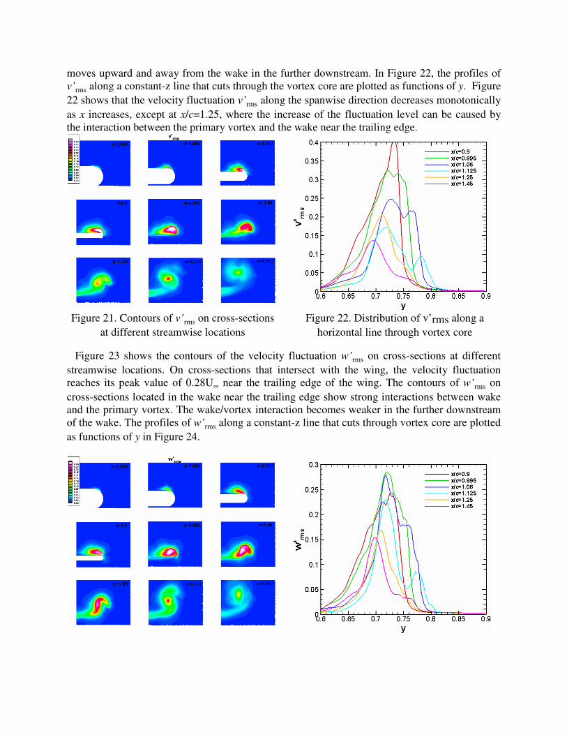
Figure 23 shows the contours of the velocity fluctuation w’rms on cross-sections at different

streamwise locations. On cross-sections that intersect with the wing, the velocity fluctuation

reaches its peak value of 0.28U∞ near the trailing edge of the wing. The contours of w’rms on

cross-sections located in the wake near the trailing edge show strong interactions between wake

and the primary vortex. The wake/vortex interaction becomes weaker in the further downstream

of the wake. The profiles of w’rms along a constant-z line that cuts through vortex core are plotted

as functions of y in Figure 24.

Figure 23. Contours of w’rms on cross-sections

at different stremwise locations

Figure 24. Distribution of w’rms along a


The contours of the components of Reynolds stress u’v’, u’w’, and v’w’ are plotted on cross-

sections with different streamwise locations in Figure 25, Figure 27, and Figure 29, respectively. .

Figure 26, Figure 28, and Figure 30 show the profiles of the three components of the Reynolds

stress along a line with constant z through vortex core as functions of y. The contours on the

cross-sections shown in Figure 25 indicate that the separated shear layer has maximum Reynolds

shear stress u’v’. The two–lobe structure identified by opposite sign of Reynolds shear stress u’v’

in the vortex core can be seen at cross-sections over the wing surface and in the wake. Similar

observation has also been found by the experiment (Chow, et al, 1997). In the wake of the wing,

the Reynolds shear stress u’v’ decreases rapidly along the axial direction. In Figure 29, the

contours on the cross-section also indicate that the separated shear layer has the maximum

Reynolds shear stress u’w’. Again, the two–lobe structure identified by the opposite sign of u’w’

in the vortex core can be seen at cross-sections over the wing surface and in the wake. The u’w’

component of the Reynolds stress decreases rapidly along the axial direction in the wake. In

Figure 29, the contours of the v’w’ show a four-leaf clove pattern which was also observed in the

experiment (Chow, et al, 1997). This pattern becomes more clear in the wake where the

distortion effect of the shear layer vanishes. The distribution of v’w’ in the plot indicates that

strong turbulent activity appears in the center of the vortex core over the wing surface. The

Reynolds stress v’w’ also decays along the axial direction in the wake

Figure 25. Contours of Reynolds shear stress

component u’v’ on cross-sections at different

streamwise locations

Figure 26. Profiles of Reynolds shear stress

u’v’ along a horizontal line through vortex core


component u’w’ on cross-sections at different



u’w’ along a horizontal line through vortex

core


component v’w’ on cross-sections at different



v’w’ along a horizontal line through vortex

core

The contours of means strain rate

∂

∂+

∂

∂−

y

w

z

v is displayed in Figure 31. Compared with the

corresponding Reynolds shear stress shown in Figure 29, the Reynold stress is not aligned with

the mean strain rate, which is consistent with the finding in Chow’s experiment. This indicates

the strong anisotropy in the vortex.

Figure 31. Contours of mean strain rate

∂

∂+

∂

∂−

y

w

z

von cross-sections at different


Figure 32 shows the contours of turbulence kinetic energy on cross-sections at different

streamwise locations. The profiles of turbulence kinetic energy along a horizontal line through

vortex core are plotted as functions of y in Figure 33. The maximum turbulence kinetic energy

occurs in the separated shear layer near the wing tip, as shown in Figure 32. After the primary

vortex is formed, the peak turbulence kinetic energy appears at the center of the vortex core. In

the wake, the turbulence kinetic energy decreases rapidly along the axial direction. In Figure 33,

on the profiles corresponding to the cross-sections at x/c=1.06 and 1.125, the second peak

reflects the wake effect.

Figure 32. Contours of turbulence kinetic

energy on cross-sections at different


Figure 33. Profiles of turbulence kinetic energy

along a horizontal line through vortex core

The distribution of pressure perturbation reveals the propagation of acoustic waves away from

the wing tip, as shown in Figure 34 where the contours of RMS of pressure fluctuation are

plotted on cross-sections with different streamwise locations. The pressure perturbations thus the

acoustic waves are closely related to the fluctuations in the tip vortex and the separated turbulent

shear layer. The formation of the primary tip vortex is considered as a major source of the noise

associated with the acoustic waves.

Figure 34. Contours of RMS of pressure fluctuation

5. LES Results and Discussions

Large Eddy Simulations with filtered-structure function subgrid model (Ducros, et al, 1996) on

two sets of grids are also performed. The numbers of grid are 1024 80 144× × (around 12 millions)

in coarse grid simulation and 1024 160 160× × (around 26 millions) in fine grid simulation. The fine

grid is the same as the one used in ILES.

Figure 35 and Figure 36 show the pressure contours and velocity vectors on the cross-sections

at different streamwise locations. Compared with the ILES result shown in Figure 6, in fine grid

LES, primary and secondary votices have the similar features as those captured in ILES, while

coarse grid result shows fewer small structures and the primary vortex is less deformed. The

primary vortex dissipate more rapidly in coarse grid LES.

(a)

(b)

(c)

(d)

(e) (f)

Figure 35. Instantaneous (t= 3.55c/U∞ ) pressure contours and velocity vectors in the cross

planes at different streamwise locations (a) x/c=0.9; (b) x/c=0.995; (c) x/c=1.06; (d) x/c=1.125;

(e) x/c=1.25; (f) x/c=1.45. Fine grid LES.

(a)

(b)

(c)

(d)

(e)

(f)

Figure 36. Instantaneous (t= 3.75c/U∞ ) pressure contours and velocity vectors in the cross

planes at different streamwise locations (a) x/c=0.9; (b) x/c=0.995; (c) x/c=1.06; (d) x/c=1.125;

(e) x/c=1.25; (f) x/c=1.45. Coarse grid LES.

Figure 37 shows the time history of axial velocity at the streamwise locations ranging from 0.9c

to 1.452c inside the vortex core. Solid lines represent ILES result and dashed lines are from fine

grid LES result. We can see that fine grid LES shows the similar broadband spectrum feature of

the velocity fluctuations as that from ILES. As the fine grid LES starts from the intermediate

solutions from ILES (at about t=2.475c/U∞ ), the solutions at the initial stage in LES match ILES

solutions.

Figure 37. Time history of axial velocity at different streamwise locations inside the vortex core,

comparison between ILES and LES. Solid lines: ILES; Dashed lines: fine grid LES.

The time averaged profiles of the axial vorticity along a horizontal centerline at different

streamwise locations are shown in Figure 38. The comparison between ILES and LES shows that

LES model has little effect on the mean flow quantity in the wake region downstream the trailing

edge, while over the wing surface, the vorticity strength predicted by LES is stronger. This

indicate that the grid resolution is high enough in the wake region so that LES model is not in

effect, while over the suction surface where turbulence is more intense, the grid resolution in

ILES is not high enough, thus the LES model takes effect. The comparison between the fine

grid LES and coarse grid LES shows large difference in both near surface region and wake

region, which indicates that the resolution of the coarse grid is poor in both regions.

(a) Comparison between ILES and LES

(b) Comparison between fine and coarse LES

Figure 38. Distribution of axial vorticity along a horizontal line through vortex core

Figure 39 shows contours of the time averaged axial vorticity in cross planes at different

streamwise locations. It is obvious that because of the poor grid resolution, the primary vortex

dissipates more rapidly in coarse grid LES. The vortex behavior predicted from the fine grid LES

(a) shows the similar feature as that from ILES (Figure 11)

(a) fine grid LES

(b) coarse grid LES

Figure 39. Contours of mean axial vorticity in cross planes at different locations

The pressure coefficient profiles along the center lines of the vortex core, the contours of mean

(time averaged) pressure on the cross-sections at different streamwise locations and Distribution

of velocity component in z direction along a horizontal line through vortex core are shown in

Figure 40, Figure 41 and Figure 42. ILES result and fine grid LES result are close to each other

in the wake region. Coarse grid is too dissipative and not fine enough to resolve large gradient

profiles.

(a) Comparison between ILES and LES (b) Comparison between fine and coarse LES

Figure 40. Distribution of pressure coefficient along a horizontal line through vortex core

(a) fine grid LES

(b) coarse grid LES

Figure 41. Contours of mean pressure in cross-sections at different streamwise locations



Figure 42. Distribution of velocity component in z direction along a horizontal line through

vortex core

The comparisons of the components of Reynolds stress, turbulence kinetic energy, and mean

strain rate between ILES and fine grid LES, fine grid LES and coarse grid LES are shown in

Figure 43 through Figure 57. For most turbulent statistic quantities, larger differences between

ILES and fine grid LES are observed over the wing surface where turbulence fluctuations are

strong. In the wake region, two solutions show less difference except for Reynolds shear stress.

These findings suggest that the grid resolution over the wing surface needs to be improved more

than that in the wake region where turbulence fluctuations start to decay. Currently a finer grid

ILES is ongoing. The result will be used to evaluate the solution from the fine grid LES and

check the grid convergence property of ILES.



Figure 43. Distribution of u’rms along a horizontal line through vortex core

(a) fine grid LES

(b) coarse grid LES

Figure 44. Contours of u’rms on cross-sections at different streamwise locations



Figure 45. Distribution of v’rms along a horizontal line through vortex core

(a) fine grid LES (b) coarse grid LES

Figure 46. Contours of v’rms on cross-sections at different streamwise locations


Figure 47. Distribution of w’rms along a horizontal line through vortex core


Figure 48. Contours of w’rms on cross-sections at different stremwise locations


Figure 49. Profiles of Reynolds shear stress u’v’ along a horizontal line through vortex core

(a) fine grid LES

(b) coarse grid LES

Figure 50. Contours of Reynolds shear stress component u’v’ on cross-sections at different




Figure 51. Profiles of Reynolds shear stress u’w’ along a horizontal line through vortex core

(a) fine grid LES

(b) coarse grid LES

Figure 52. Contours of Reynolds shear stress component u’w’ on cross-sections at different



Figure 53. Profiles of Reynolds shear stress v’w’ along a horizontal line through vortex core


Figure 54. Contours of Reynolds shear stress component v’w’ on cross-sections at different




Figure 55. Profiles of turbulence kinetic energy along a horizontal line through vortex core


Figure 56. Contours of turbulence kinetic energy on cross-sections at different streamwise

locations

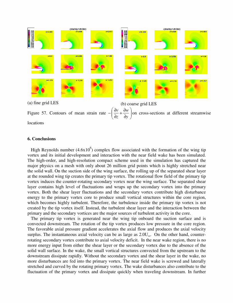
(a) fine grid LES

(b) coarse grid LES

Figure 57. Contours of mean strain rate

∂

∂+

∂

∂−

y

w

z

von cross-sections at different streamwise

locations

6. Conclusions

High Reynolds number (4.6x106) complex flow associated with the formation of the wing tip

vortex and its initial development and interaction with the near field wake has been simulated.

The high-order, and high-resolution compact scheme used in the simulation has captured the

major physics on a mesh with only about 26 million grid points which is highly stretched near

the solid wall. On the suction side of the wing surface, the rolling up of the separated shear layer

at the rounded wing tip creates the primary tip vortex. The rotational flow field of the primary tip

vortex induces the counter-rotating secondary vortex near the wing surface. The separated shear

layer contains high level of fluctuations and wraps up the secondary vortex into the primary

vortex. Both the shear layer fluctuations and the secondary vortex contribute high disturbance

energy to the primary vortex core to produce small vortical structures within the core region,

which becomes highly turbulent. Therefore, the turbulence inside the primary tip vortex is not

created by the tip vortex itself. Instead, the turbulent shear layer and the interaction between the

primary and the secondary vortices are the major sources of turbulent activity in the core.

The primary tip vortex is generated near the wing tip onboard the suction surface and is

convected downstream. The rotation of the tip vortex produces low pressure in the core region.

The favorable axial pressure gradient accelerates the axial flow and produces the axial velocity

surplus. The instantaneous axial velocity can be as large as 2.0U∞. On the other hand, counter-

rotating secondary vortex contribute to axial velocity deficit. In the near wake region, there is no

more energy input from either the shear layer or the secondary vortex due to the absence of the

solid wall surface. In the wake, the small vortical structures convected from the upstream to the

downstream dissipate rapidly. Without the secondary vortex and the shear layer in the wake, no

more disturbances are fed into the primary vortex. The near field wake is screwed and laterally

stretched and curved by the rotating primary vortex. The wake disturbances also contribute to the

fluctuation of the primary vortex and dissipate quickly when traveling downstream. In further

downstream, the tip vortex becomes more stable and flow in the core region is more

axisymmetric.

On the cross-sections that are intersected with the wing, the peak values of velocity

fluctuations are found over the suction side of the wing where the shear layer separates from the

rounded wing tip. The high level fluctuations are wrapped up into the vortex core and convected

downstream. In the wake region, the peak of velocity fluctuation appears in the center of the

vortex core and fluctuation level decreases rapidly downstream along the axial direction.

Pressure perturbation field shows that the noise source locates in the near tip region and

acoustic waves propagate away from the wing tip. The fluctuations inside the tip vortex

contribute to the pressure perturbations.

Three numerical simulations have been performed. One is fine grid (26 millions) LES without

model which we call implicit LES (ILES). The second one is fine grid (26 millions) LES with

filtered-structure function subgrid model and the third one is course grid (12 millions) LES with

the same subgrid model. The computation shows fine grid ILES and LES results are similar in

the wake and different near the wall, which shows more resolution is needed to resolve the near

wall small vortices. The coarse grid LES shows too dissipative to tip vortex which is dissipated

too fast after shedding. This also demonstrates the second order subgrid model is inconsistent to

a six-order compact scheme.

We would like to make some comments on low order LES with low order subgrid models.

The fundamental idea of using LES is to resolve large scales as much as possible. Therefore, low

order scheme, such as second order central or bias difference scheme, is not appropriate for LES

due to their low order accuracy and low resolution although we are aware that many LES work

with low order scheme have been reported, and high order compact scheme is preferred for flow

transition and turbulence. Most LES computations require use of a subgrid model trying to get

the unresolved scales back which could be considered as truncation errors mathematically.

However, Smagorinsky model and many other subgrid models are second order with 2∆ . If we

use sixth order compact scheme for LES without model (Implicit LES), we will get sixth order of

accuracy. However, if we add the Smgorinsky subgrid model, our LES results will be

degenerated to second order of accuracy, which is really bad. A carefully designed 6th

order

subgrid model may be needed for high order LES. Therefore, second order ILES, second order

LES with second order subgrid models are not appropriate. The second order subgrid models

degenerate the original ILES results, which is six order in accuracy, to second order. This is a

critical problem to most of LES work reported. The possible solution is to increase grids in the

near wall region or develop a six order subgrid model.

Table 2 shows the orders obtained by different orders of schemes, which demonstrates the

importance of high order numerical schemes for DNS/LES.

Table 2. Orders of DNS/LES approaches

Scheme Truncation Errors Comments

Second order DNS )( 2hO Bad

Second order LES +Second order

subgrid model )( 2hO or up Bad

Sixth order LES without subgrid

model (ILES) )( 6hO Good

Sixth order LES with second order

subgrid model )( 2hO Really bad

Sixth order LES with sixth order

subgrid model )( 6hO or up Best

Acknowledgments

This work was sponsored by the Office of Naval Research (ONR) and monitored by Dr. Ron

Joslin under grant number N00014-03-1-0492. The authors also thank the High Performance

Computing Center of US Department of Defense for providing supercomputer hours.

References

[1] Choudhari and Khorrami, Computational study of porous treatment for altering flap side-

edge flow field, AIAA Paper 2003-3113, 2003.

[2] Chow, J.S., Zilliac,G.G.,Bradshaw,P., Mean and turbulence measurements in the near field

of a wingtip vortex. AIAA J. 35, 1561-1567, 1997.

[3] Chow, L.C., Mau, K., and Remy, H., “Landing Gears and High Lift Devices Airframe

Noise Research,” AIAA Paper 2002-2408, 2002.

[4] Dacles-Mariani, J., Kwak, D., Zilliac, G., Accuracy assessment of a wingtip vortex

flowfield in the near-field region. AIAA paper 96-0208, 1996.

[5] Ducros, F., Comte, P. and Lesieur, M., Large-eddy simulation of transition to turbulence in

a boundary layer developing spatially over a flat plate. J. Fluid Mech. 326, pp1-36, 1996

[6] Fleig, O., Arakawa, C., Large-eddy simulation of tip vortex flow at high Reynolds number,

AIAA Paper 2004-0261, 2004.

[7] Jiang, L., Shan, H., Liu, C., Direct numerical simulation of boundary-layer receptivity for

subsonic flow around airfoil. In: Recent Advances in DNS and LES, Proceedings of the

Second AFOSR (Air Force Office of Scientific Research) International Conference,

Rutgers, New Jersey, June 7-9, 1999.

[8] Jiang, L., Shan, H., Liu, C., Nonreflecting boundary conditions for DNS in curvilinear

coordinates. In: Recent Advances in DNS and LES, Proceedings of the Second AFOSR

(Air Force Office of Scientific Research) International Conference, Rutgers, New Jersey,

June 7-9, 1999.

[9] Khorrami, M.R., and Singer, B.A., “Stability Analysis for Noise-Source Modeling of a

Part-Span Flap,” AIAA J. Vol 37, No. 10, pp1206-1212, 1999.

[10] Labbe, O., Sagaut, P., Unsteady wake vortices simulation behind a A300 model. AIAA

paper 2003-4022, 2003.

[11] Lele, S.K., Compact finite difference schemes with spectral-like resolution. J. Comput.

Phys. 103,pp16-42, 1992

[12] Poinsot, T.J., Lele, S.K., Boundary conditions for direct simulations of compressible

viscous flows. J. Comput. Phys. 101, pp104-29, 1992.

[13] Shan, H., Jiang, L., and Liu, C., Direct numerical simulation of three-dimensional flow

around a delta wing. AIAA Paper 2000-0402, 2000.

[14] Shan, H., Jiang, L., Liu, C., Numerical simulation of flow separation around a NACA 0012

airfoil, Computers & Fluids, Vol.34, pp1096-1114, 2005.

[15] Slooff, J.W., de Wolf, W.B., van der Wal, H.M.M., and Maseland, J.E.J., “Aerodynamic

and aeroacoustic effects of flap tip fences,” AIAA Paper 2002-0848, 2002.

[16] Spekreuse, S.P., Elliptic grid generation based on Laplace equations and algebraic

transformation. J. Comp. Phys. 118, 38, 1995.

[17] Youssef, K.S., Ragab, S. A., Devenport, W. J., Gawad, A. F. A., Large eddy simulation of

the near wake of a rectangular wing. AIAA paper 98-0317, 1998.

[18] Yoon, Z.Y., Voke P.R., Implicit Navier-Stokes solver for three-dimensional compressible

flows. AIAA J. 30, pp2653-9, 1992

Large Eddy Simulation of Wing Tip Vortex in the Near Field · Department of Mathematics, University...

Documents

Transcript of Large Eddy Simulation of Wing Tip Vortex in the Near Field · Department of Mathematics, University...