
Large eddy simulations of gaseous flames in gas turbine combustion chambers

Large Eddy Simulation of Turbulent Flow and Combustion in HCCI Engines
Rixin Yu
May, 2008
Ph.D. thesis

Thesis for the degree of Doctor of Philosophy in Engineering ISBN 978-91-628-7476-6 ISSN 0282-1990 ISRN LUTMDN/TMHP--08/1060--SE © 2008 Rixin Yu and the respective publishers Divison of Fluid Mechanics Faculty of Engineering Lund University Box 118 S-221 00 LUND Sweden Printed by E-husets Tryckeri, April 2008

Preface
This thesis deals with large eddy simulation of turbulent combustion process in HCCI engines. The thesis is based on the first seven the publications list below [1-7]. The remaining publications are not included in this thesis and deal with large eddy simulation of turbulent non-premixed flames in model gas turbines [8], non-premixed flame in a pulsating combustor [9] and lifted partially-premixed flame in a laboratory scale burner [10].
1 R. Yu, X.S. Bai: A semi-implicit scheme for large eddy simulation of piston engine flows. Manuscript submitted for publication, 2008.
2 R. Yu, X.S. Bai, H. Lehtiniemi, S.S. Ahmed, F. Mauss, M. Richter, M. Aldén, L. Hildingsson, B. Johansson, A. Hultqvist: Effect of Turbulence and Initial Temperature Inhomogeneity on Homogeneous Charge Compression Ignition Combustion, SAE paper 2006-01-3318, 2006.
3 R. Yu, X.S. Bai, L. Hildingsson, A. Hultqvist, P. Miles: Numerical and Experimental Investigation of Turbulent Flows in a Diesel Engine, SAE paper 2006-01-3436, 2006.
4 R. Yu, X.S. Bai, A. Vressner, A. Hultqvist, B. Johansson, J. Olofsson, H. Seyfried, J. Sjöholm, M. Richter, M. Aldén: Effect of Turbulence on HCCI Combustion, SAE paper 2007-01-0183, 2007. Accepted for publication in SAE Transactions, Journal of Passenger Cars – Mechanical Systems, 2008.
5 R. Yu, X.S. Bai: LES of In-cylinder Turbulence and Temperature Stratification in a HCCI Engine, Proc. of ECCOMAS thematic conference on computational combustion, Delft, July 18-20, 2007.
6 R. Yu, T. Joelsson, X.S. Bai, B. Johansson: Effect of Temperature Stratification on the Auto-ignition of Lean Ethanol/air Mixture in HCCI Engine, SAE paper 2008-01-1669.
7 T. Joelsson, R. Yu, X.S. Bai, A. Vressner, B. Johansson: Large Eddy Simulation and Experiments of the Auto-ignition process of Lean Ethanol/air Mixture in HCCI Engines, SAE paper 2008-01-1668.
8 R. Yu, K.J. Nogenmyr, X.S. Bai: LES of swirling turbulent methane/air flame, Proc. of ECCOMAS thematic conference on computational combustion, Lisbon, June 21-24, 2005.
9 E. Baudoin, R. Yu, X.S. Bai, J. Hrdlicka, S.I. Moller, M. Alden: Large Eddy simulation and Measurements of Methane/Air Combustion in a Pulsating Combustor. ECCOMAS Computational Combustion Conference, Delft, The Netherlands, 2007.
10 B. Li, E. Baudoin, R. Yu, Z.W. Sun, Z.S. Li, X.S. Bai, M. Alden, M.S. Mansour: Experimental and Numerical Study of a Conical Turbulent Partially Premixed Flame, accepted by the 32nd International combustion symposium, 2008.

Abstract
This thesis deals with numerical simulations of the turbulent combustion process in Homogeneous Charge Compression Ignition (HCCI) engines. An accurate and computationally efficient Large Eddy Simulation (LES) model was developed and used throughout this thesis to investigate the development of in-cylinder turbulence, temperature stratification, onset of auto-ignition, and development of the reaction fronts. Compared with the conventional Reynolds averaged Navier-Stokes (RANS) approaches, LES has the potential of capturing the fine spatial and temporal structures in engine combustion chambers. Yet, there are several difficulties when applying LES to engine flows. It is often not possible to have the fine resolution needed for some of the flow scales in the cylinder, for example in the near-wall regions. In addition to the difficulty of resolving the flow scales there is a lack of a numerically accurate and affordable method for coupling the detailed auto-ignition chemical kinetic to the flow field simulations.
An efficient auto-ignition model is developed based on parameterization of auto-ignition history obtained from detailed chemical kinetics calculations. The model is implemented to the LES solver and used to improve the understanding of the fundamental physical and chemical process in HCCI engines. First, an experimental engine with a rectangular shaped combustion chamber operating at low speed was chosen as a test case for validation of the LES model. Fairly good agreement between the LES results and the PIV (particle image velocimetry) experiments are found with respect to the cycle averaged mean flow field and turbulence fluctuations. Several spatial and temporal average methodologies were examined based on one single cycle LES data to characterize the mean flow and turbulence.
The LES model is then used to study several HCCI experimental engines that have realistic cylinder geometry and engine speed. With very high spatial and temporal resolution the LES model successfully simulated the development of flow structures during the different strokes of the engine cycle. The effect of intake gas, residual gas, wall temperature, and piston geometry on the turbulent flow and temperature stratification was quantified. The LES revealed fundamental aspects of HCCI combustion, and its dependence on engine cylinder geometry, cooling, and operational conditions such as intake gas preheating. The LES results indicated that the effect of the geometry is not to alter the production of in-cylinder turbulence, but instead, to affect the heat transfer between the in-cylinder gas and the bowl wall. Compared with flat piston engines, the bowl-in-piston engine generates a high level of temperature stratification in the cylinder which leads to an earlier auto-ignition. By controlling the intake gas temperature to obtain the same auto-ignition timing, it was found that the combustion duration was increased with the bowl-in-piston as compared to a flat piston. This phenomenon was first observed in HCCI engine experiments. With the present LES study a clearer understanding of the flow-heat transfer-reaction coupling was obtained.
Systematic LES studies carried out in this thesis showed that the effect of turbulence can be important for the formation and destruction of the temperature stratification in the engine cylinders. Turbulence can decrease the temperature inhomogeneity in the bulk flow far away from the walls. Therefore residual gas/intake gas induced temperature stratification is suppressed by strong turbulence eddy motion. On the other hand, turbulence eddy motion in the wall boundary layers is responsible for the generation of temperature stratification in the cylinder. Turbulence was found to be able to affect the reaction front propagation directly in HCCI engines under conditions that the large eddies and the hot reaction zones are comparable in size.

Acknowledgements
This work is financially sponsored by the Swedish Energy Agency through the Competence Center KC-FP at Lund University, and also partially supported by Swedish Research Council (VR) and the Centre of Combustion Science and Technology (CECOST). Most of computations in this work are carried out at the computing center (LUNARC) in Lund University.
First of all, I would like to thank my main supervisor Prof. Xue-Song Bai for the opportunity of PhD study. Thanks for introducing me into the field of turbulent combustion. I am greatly benefited from a lot of discussions and also the trust in supporting me working on the LES code.
Thanks Prof. Laszlo Fuchs, Dr. Johan Revstedt for the knowledge I learned from their courses. Dr. Edward S. Blurock and Dr. Lei Wang are thanked for cross-reading and commenting on my thesis. My gratitude goes also to Prof Zhi-Qiang Zhu for leading me into the research field.
Thanks to Karl-Johan Nogenmyr, Tobias Joelsson, Eric Baudoin for being my close colleagues and also cooperating to publish together. I am grateful to Dr. Andreas Vressner, Prof Bengt Johansson, Dr. Anders Hultqvist, Dr. Paul Miles, Dr. Mattias Richter and Prof. Marcus Aldén for sharing their nice engine experiments, and Harry Lehtinirmi, Sayeed Ahmed and Prof. Fabian Mauss for collaboration in the chemical kinetics modeling.
Thanks many friends: Takamasa Ito, Dragan Stankovic, Raik Orbay, Andre Hildebrandt, Magnus Åberg, Philip Evegren, Torbern Klason, Ping Wang and many more. Thanks for a lot of nice time staying together.
Last but not least I would like to thank my wife Lixia and my parents for their constant loves and supports.

Table of Contents
1 Introduction ...........................................................................................................1 1.1 Fundamental understanding of HCCI combustion process ...........................................1 1.2 Modeling of HCCI combustion process........................................................................3 1.3 Scopes of this thesis work .............................................................................................4
2 Mathematical description of flows and combustion in HCCI engines .............5 2.1 Governing equations .....................................................................................................5 2.2 Modeling of Ignition Chemistry....................................................................................6
2.2.1 The progress variable based tabulation model...................................7 2.2.2 Generation of ignition library ............................................................7 2.2.3 Correction for the Endothermic Reaction ..........................................8 2.2.4 Comparison with multi-zone method.................................................9
2.3 Spatial filtering for large eddy simulation...................................................................10 2.4 Governing equations in deforming coordinate ............................................................11
General form of the transport equations .................................................12 Thermodynamic relations .......................................................................13
2.5 Boundary conditions ...................................................................................................14 2.5.1 Modeling of flow through opening valves.......................................14
Geometrical representation .....................................................................14 Volume and mass flow rate through intake valves..................................15 Determination of the normal velocity u#.................................................15
2.5.2 Wall boundary condition..................................................................16 2.5.3 Initial conditions ..............................................................................16
3 Numerical methods .............................................................................................17 3.1 Variable time step........................................................................................................17 3.2 Staggered Cartesian Grid ............................................................................................17 3.3 Spatial discretization ...................................................................................................18
3.3.1 Fifth order WENO scheme ..............................................................18 3.3.2 The Deferred Correction method .....................................................20
3.4 The predictor-corrector method...................................................................................20 3.4.1 The predictor step ............................................................................21
Step 1: Calculation of Pn+1(Predictor) .....................................................21 Step 2: Transport of enthalpy and progress variable (Predictor) ............21 Step 3: The Continuity Equation (Predictor) ..........................................22 Step 4: Momentum transport (Predictor) ................................................22 Step 5: Pressure Poisson equations (Predictor).......................................23
3.4.2 The corrector step ............................................................................23 Step 6: Transport of enthalpy and progress variable (corrector).............23 Step 7: Pressure Poisson equation (corrector).........................................24
3.5 Further numerical issues .............................................................................................24 3.5.1 Convergence affected by round-off error.........................................24 3.5.2 Multi-Grid method handling high grid aspect ratio .........................25 3.5.3 Diffusive stability Limit...................................................................26
3.6 Features of the in-house LES codes used in this thesis ...............................................27 3.7 Validation of the LES solver .......................................................................................28
3.7.1 Instantaneous vorticity field.............................................................29 3.7.2 Mean tumble flow ............................................................................30
4 Quantification of in-cylinder turbulence and combustion ..............................32

4.1 Velocity vector field, streamlines, and vorticity field..................................................32 4.2 The λ2 method .............................................................................................................33 4.3 Statistical description of in-cylinder flows..................................................................35
Ensemble average approach....................................................................35 Spatial filtering approach........................................................................35 Pressure trace, heat release rate, and normalized cumulative heat release.................................................................................................................35
5 Results and discussions .......................................................................................37 5.1 Instantaneous flow structures and temperature stratification ......................................37
5.1.1 Intake stroke.....................................................................................38 5.1.2 Compression stroke..........................................................................41
Flow structures........................................................................................41 Temperature field and hot zone...............................................................43
5.1.3 Expansion stroke..............................................................................44 5.2 Evolution of turbulence...............................................................................................44 5.3 Evolution of temperature inhomogeneity....................................................................46
5.3.1 Intake stroke.....................................................................................47 5.3.2 Compression stroke..........................................................................49
5.4 Effect of turbulence and temperature inhomogeneity on HCCI combustion ..............50 6 Summary of papers .............................................................................................56 7 Conclusion and perspectives ..............................................................................59 8 References ............................................................................................................61

Chapter 1: Introduction
1
1 Introduction
In the past ten years, homogeneous charge compression ignition (HCCI) combustion has received great interests from the combustion research community and the engine industry [1, 2]. HCCI combustion processes have the potential of not only providing high efficiency that is similar to diesel engine combustion, but also producing much lower emissions of NOx and soot. HCCI combustion is different from the two well-known combustion processes, namely the premixed flame propagation found in spark ignition gasoline engines and diffusion flames found in diesel engines. In a premixed flame, a thin reaction layer propagates in the fuel/air mixture; the propagation speed is governed by the chemical reactions and the diffusion of species between the reaction zone and the preheat zone [3]. In a diffusion flame, chemical reactions occur also in very thin layers and the combustion process is governed by the diffusion of fuel and air to the reaction zones and the heat transfer to cold fuel and air streams [4]. In both turbulent premixed and diffusion flames, turbulence length scales are often larger than the thickness of the reaction layers, thus one of the main effects of turbulence is to wrinkle the reaction layers and to increase the surface area of the reaction layers and the fuel conversion rate. At high intensity and small scale turbulence conditions, turbulence can also cause local extinction of the chemical reactions. Comprehensive understanding and proper modeling and predicting the turbulence/flame interaction have been very crucial for designing spark-ignition engines (premixed flames) and diesel engines (diffusion flames).
HCCI combustion represents a third mode of combustion. Fuel and air are premixed before ignition (which is similar to premixed flames), however, the ignition occurs due to compression of the fuel/air mixture. Thus, ideally, ignition occurs homogeneously in the entire combustor. In such cases, combustion is governed by chemical kinetics. However, simulations of HCCI combustion based on only the chemical kinetics have failed to repeat the experimental observations. Experimental evidence shows that the ignition kernels are rather inhomogeneous with the reaction fronts propagating in space and that turbulence affects the reaction fronts significantly (e.g. [5]). The strong interaction of the reaction fronts with turbulence, which behaves in a rather unsteady and chaotic way, has made the process rather difficult to control, especially with varying loads and other operation conditions.
1.1 Fundamental understanding of HCCI combustion process
HCCI combustion was first reported by Onishi et al [6]. Since then (in particular after 1996) many experimental studies on the subject have been carried out (e.g., [1, 5, 7-12]). Earlier experiments were focused on the in-cylinder pressure measurement and engine performance (e.g. emissions in the exhaust gas). Little was known about the detailed reaction layer structures. The auto-ignition of homogeneous mixture of fuel and air was believed to be homogeneous in space, so the progress of heat release depended only on the chemical reaction progress. This assumption has led to the development of several models for the simulation of the combustion process [13, 14]. These models however, have difficulties in predicting the effect of turbulence on the combustion process, e.g., the elevated combustion duration at higher turbulence levels.
Recently, new discoveries were made with the advancement of sophisticated laser diagnostics. In particular it has been found that there are fine ignition-kernels present in HCCI combustion [5, 10-12]. There are a number of possible mechanisms that account for the observed ignition kernels:
• intrinsic instability of the combustion process; • inhomogeneity of the fuel/air/exhaust gas mixing, • inhomogeneity of the initial temperature, and • wall effects.

Chapter 1: Introduction
2
It is natural that inhomogeneity of the fuel/air/exhaust gas mixture would cause inhomogeneous ignition. However, experimentally it has been found that with a very homogeneous mixture there are still inhomogeneous auto-ignition kernels [5, 10, 11]. Figure 1 shows measurements [12] compared to a numerical study (paper 2) of the distribution of OH radicals and formaldehyde (CH2O) in an optical experimental HCCI engine. The fuel (50% n-heptane and 50% iso-octane) and air were premixed in a tank outside of the experimental engine. The homogeneous mixture was injected to the engine after complete mixing. The images were taken shortly after the auto-ignition of the fuel/air mixture using planar laser-induced fluorescence (PLIF) technique. As seen from the experiments, owing to the homogeneous mixture the first stage ignition that forms formaldehyde is rather homogeneous in space. However, the second stage ignition that forms OH radicals with major heat release is not homogeneous at all (see first column from left, Fig.1, CAD larger than +10 degrees).
Figure 1. First column from left: Single-shot PLIF images from onset of cool flame first stage ignition until the end of the main ignition. Formaldehyde is shown in grey and OH is shown in red. Last three columns from left: LES predicted instantaneous distribution of formaldehyde (CH2O), OH, temperature and fluid trace lines (Exp results
are taken from Colin et al. 2003, LES results are taken from paper 2).
Of those possible mechanisms, studies of the effect of initial temperature inhomogeneity are the only one that has been carried out to certain extent. Earlier works can be traced back to those by Russian scientists in 1930s – 1960s, see a review by Zel’dovich [15]. Based on theoretical studies of the propagation of reaction fronts in an idealized one-dimensional infinitely long domain, Zel’dovich outlined three distinct regimes of reaction front propagation for a mixture with non-homogeneous initial temperature: detonation, deflagration, and spontaneous propagation. Detonation leads to engine knock that should be avoided; it occurs for example in homogeneous mixture with very small temperature gradient. Deflagration front propagation (known as flame propagation) is controlled by both chemical reactions and diffusion of heat and mass between the reaction front and the unburned mixture; spontaneous propagation is however due to the difference of auto-ignition delay between adjacent points. This work is continued recently by using more precise chemical kinetics and computational methods. For example, Sankaran and Im [16] carried out a numerical calculation of iso-octane ignition in an atmospheric pressure counter flow configuration, confirming the effect of temperature gradient and mixing rate on the overall
-17
+15
+10
+2
-7
Exp. grey=CH2O, red=OH
CAD

Chapter 1: Introduction
3
ignition characteristics. In the present thesis, more complex three dimensional engine configurations have been considered (see Fig.1). Large eddy simulation (LES) method was used to resolve the length scales down to Taylor micro-scales and thereby capturing certain fine ignition kernel structure. Homogeneous mixture was assumed in the LES; the initial temperature was, however, not assumed to homogeneous. This has led to inhomogeneous ignitions kernels in both the first stage and second stage ignitions (paper 2). From these results it is clear that the initial temperature inhomogeneity is at least partially responsible for the onset of the fine reaction front structures in HCCI.
Two fundamental questions are how these fine ignition kernels develop in space and time and how these developing fronts affect the overall combustion process. These questions are of central importance for interpretation of the main heat release, temperature and pressure development in HCCI engines, as well as for modelers to develop simulation models. Many researchers [1, 13, 14] assumed that the inhomogeneous temperature causes merely inhomogeneous ignition delay in space; the ignition kernels are merged later. Based on this understanding, the entire flow field can be treated as a well-stirred reactor; the combustion process is controlled by chemical kinetics and turbulence affects the process mainly by mixing of reactants and heat. This is however contradicting earlier experimental evidences which showed that the small ignition kernels may propagate in a way similar to flame propagation. For example, in [17] it is shown that the reaction fronts are highly irregular and wrinkled. The irregularly wrinkled boundary surface resembles the wrinkled flame surfaces in turbulent premixed flames [18, 19]. To look further into the details of this process, more theoretical, numerical and experimental investigations are needed.
1.2 Modeling of HCCI combustion process
Although many experimental results on HCCI process are available, theoretical analysis and models for simulation of HCCI combustion are less well developed. As discussed in the previous section earlier HCCI modeling work was mainly based on the assumption that the process is controlled by chemical kinetics. The combustion chamber was assumed to be a single zone well-stirred reactor (zero-dimensional in space) that has a single pressure and temperature [7, 9, 20]. Detailed chemistry was incorporated in the models. These models can qualitatively predict the ignition delay time for different fuels, including the cool flame stage, sensitivity to compression ratio, equivalence ratio, etc. [21]. However, single zone models greatly overestimated the rates of heat release and showed poor agreement with the experimentally obtained in-cylinder pressure development history. The deficiencies of the single zone models are due to their inability to account for the temperature gradient within the mixture [22].
Multiple zone models that allow certain spatial variations have been developed [14, 22, 23]. In the multi-zone model, the flow motion was typically simulated using CFD codes with k-ε turbulence closure; the chemistry was resolved on much coarser zones than the CFD grid, typically ten zones in total. Simulations with ten zones for the chemical kinetics yield improved results compared to single zone models. However, the prediction of combustion products such as CO was found to be an order of magnitude lower than the experiments [22, 23]. Flowers et al. [14] showed that a great number of zones are required to resolve the detailed emissions.
Kraft et al. [13] suggested a stochastic reactor model to account for the spatial temperature gradient. The flow field was still modeled as single zone. Species concentrations and temperature were assumed to vary randomly in space. Diffusion induced by turbulence mixing is described by the IEM (interaction by exchange with the mean) model. The prediction of CO and unburned hydrocarbons were shown to be better than the single-zone model. However, the fact that the stochastic model needs the input information of turbulence that is not computed by the method itself limits the application of the stochastic reactor model to engine simulations.

Chapter 1: Introduction
4
1.3 Scopes of this thesis work
As discussed above, there are significant amount of experimental works on the HCCI combustion process. However, basic understanding of the fine ignition/reaction structures and the interaction of turbulence eddies with these fine structures is very limited. This is because of the lack of theoretical analyses and spatially resolved numerical simulations of HCCI combustion. In continuing attempts to simulate HCCI combustion, the flow field has been, at best, modeled using second order moment closure (such as k-ε model, for example [24, 25]). This approach has been limited because of the difficulty in constructing models for Reynolds stresses and turbulent transport fluxes. In addition, the closure of the turbulent mean reaction rate of species is a well-known difficulty. In order to examine the details of the HCCI combustion process a more appropriate approach such as large eddy simulation (LES) should be used.
The objectives of this thesis work are:
• To scrutinize the fundamental aspects of HCCI combustion, in particular the effect of turbulence micro-scale eddies on the onset and development of the ignition kernels. The currently often used assumption that turbulence has minor effect on the ignition kernels is to be carefully examined. The detailed ignition kernel structure and its dynamics will be examined.
• To develop an efficient and accurate numerical method for doing LES of the engine flow and the combustion process in HCCI engines. The numerical method will be designed to handle the special numerical issues brought by the engine system - such as rather homogenous turbulence field, the deforming computational domain, large gradients in both flow and density field. The numerical method will be implemented as a LES code.
• To use the developed LES code to simulate the development of turbulence in the cylinder and the evolution of temperature stratification; the effect of residual gas temperature, turbulence level, the intake gas temperature and wall temperature as well as the wall geometry on the in-cylinder turbulence and temperature stratification.
The thesis is arranged as follows. In Chapter 2, the engine system is described mathematically - the governing equations together with boundary conditions are presented. In Chapter 3, the numerical methods for solving the governing equation are described in detail. LES generates three dimensional and temporal resolved data that describe the development of the flow, heat transfer, and combustion process. However, it is not trivial how to utilize and analyze the data. In Chapter 4, several approaches for quantification of the flow structures and combustion process are discussed. The numerical results are presented in detail in the attached papers. Some highlights of the results are also presented in Chapter 5. In Chapter 6 and 7, a summary of papers is attached in the appendix and conclusions of this thesis work and future perspectives are presented.

Chapter 2: Mathematical description
5
2 Mathematical description of flows and combustion in HCCI engines
The engine flow system is governed by the compressible Navier-Stokes (N-S) equations which can be applied to both high and low speed flows. High flow speed inside the engine can exist under certain conditions. For example, when large pressure difference is presented between the two sides of a valve in the moment of valve opening, the flow speed through the valve can be quite high for a short period of time. The bulk flow speed in the engine cylinder, however, is typically low throughout the engine cycle.
In this work our interests are limited to the engine flow with low speed (maximum Mach number around 0.3); the low Mach number assumption is therefore used to simplify the equations [26]. In the low Mach number assumption the acoustic effect is neglected, and the physical pressure can be split into two parts: a thermodynamic pressure P and a hydrodynamic pressure p. The thermodynamic pressure P is constant in space and only changes in time. It is this thermodynamic pressure that is used in the equation of state to relate the gas density with the temperature. The hydrodynamic pressure p, on the other hand, is used in the pressure-gradient terms in the momentum equations. With low Mach number assumption the stiffness due to the coexistence of high speed acoustic waves and low speed flow is removed, the computational efficiency can thus be greatly improved comparing with the full compressible N-S equations.
2.1 Governing equations
Let ui denote the velocity components of the in-cylinder gas mixture in Cartesian coordinates xi (i=1,2,3); let ρ, T and h represent the density, temperature and enthalpy of the gas mixture. The governing equations for the fluid flow are the result of conservation of mass, momentum and energy. They can be written in tensor form as follows:
0j
j
uρt x
ρ∂∂ + =∂ ∂
(1)
Equation (1) is the continuity equation for single phase fluid flows. The Einstein summation rule is used in Equation (1) and equations below.
The species transport equations can be written as
, 1j ii ii i
j j j
ρu YρY YρD ω i , N
t x x x
∂∂ ∂∂+ = + = ∂ ∂ ∂ ∂ … (2)
where Yi is the mass fraction of species i. N is the total number of species in the gas mixture. Di is the diffusion coefficient of species i. iω is the reaction rate of species i.
The momentum conservation equations are
( 1 2 3)i j iji
j i j
ρu u τρu p i , ,t x x x
∂ ∂∂ ∂+ = − + =∂ ∂ ∂ ∂
(3)
where the viscous stress tensor can be written as
23
ji kij ij
j i k
uu uτ µ δ µ
x x x ∂∂ ∂
= − − ∂ ∂ ∂ (4)

Chapter 2: Mathematical description
6
As noted, the momentum equation of a reactive flow is identical to the counterpart of the non-reactive flow.
The energy conservation equation in terms of enthalpy can be written as
1
11 :N
i i rii
Dh DP ρα h ρα h Y Q vDt Dt Le
ρ τ=
− = ∇ ⋅ ∇ − − ∇ + + ∇
∑ (5)
where Lei is the Lewis number of species, defined as
ii
αLeD
≡ (6)
Lewis number represents the ratio of thermal diffusion (α ) to mass diffusion (Di). The Lewis number in a combustion system may be assumed to be unity.
The last two terms on the r.h.s. of equation (5) are the source terms corresponding to the radiative heat transfer and viscous dissipation of energy, respectively. They can be neglected in the in-cylinder engine flow simulations.
The equation of state and the calorific equation of state are used to relate the temperature, species mass fractions and enthalpy with the thermodynamic pressure:
1
Ni
ui i
YP R T
Wρ
=
= ∑ (7)
0,
ref
T
i i i i p iT
h Y h Y h c dT = = + ∫ (8)
where Ru is the universal gas constant; Wi is the molecular weight of species i; 0ih is the enthalpy
of formation at the standard reference condition refT =298K and ,p ic is the heat capacity of species i.
2.2 Modeling of Ignition Chemistry
Auto-ignition is a complex chemical process involving a generally large number of species and elementary reactions. For example, a mechanism with fuel as a blend of iso-octane and n-heptane even after lumping can still contain 203 species and 2019 elementary reactions [27]. Furthermore many intermediate species are short lived, which renders the ignition system mathematically stiff. For accurate prediction elaborate numerical method must be applied and the high computational cost is unavoidable.
In HCCI process the reaction occurs in a flowing gas; the problem is severely complicated by the coupling of chemistry and flow transport. If a CFD calculation is directly coupled with chemistry, not only large numbers of transport equations are required to solve for all the species but also the heavy chemistry integration is to be performed at each of the CFD cells. The computation cost for this is generally unaffordable. Aceves et al. [28] estimated that coupling of detailed chemical kinetics with 200 reactive species using a CFD grid of one million cells would require more than a decade to obtain a single cycle data with a 2 GHz single processor computer; for the CFD flow simulation it requires only a few days. To consider CFD-chemistry coupling, simplification must be made in the numerical models.

Chapter 2: Mathematical description
7
2.2.1 The progress variable based tabulation model
A progress variable model similar to that proposed in [29-31] is used for integrating the ignition chemistry into CFD simulation. The model can be used for ignition of non-homogeneous mixture. However, only the reduced version for homogenous mixture is used in this work.
The transient ignition process is described by a progress variable defined as
* *
** *
( ) (0)( ) , ( ) ( ( ), )( ) (0) i uh hc h h Y Th h
ττ τ ττ∞
−= =−
(9)
where *( )h τ is the sensible enthalpy of the mixture at time τ (the enthalpy at standard state Tu=298K ). τ =0 means the unburned state while τ∞ denotes completed burned state. The progress variable ( )c τ is the normalized cumulative heat release. The progress variable has been used for modeling of diesel engine ignition [29], where a transport equation for c has been derived. In LES the spatial filtered progress variable equation reads
( )jj j
j j j j
u cc c u c u c ct x x Sc x x
ρρ µρ ρ ρ ρ ∂∂ ∂ ∂ ∂ + = + − + ∂ ∂ ∂ ∂ ∂
(10)
where /c dc dτ= ; it is tabulated as function of progress variable (c), total enthalpy (h) and thermodynamic pressure (P) from calculation of auto-ignition using detailed chemistry, the construction of the ignition library for c-rate will be described in the following section.
2.2.2 Generation of ignition library
The ignition library for the c method is computed based on a series of constant-pressure ignition processes. At fixed pressure P and enthalpy h, the process of constant-pressure ignition of a homogenous mixture is a pure function of time τ. For example the temperature, k-species mass fractions can be written as:
( ; , )T P hτ , ( ; , )kY P hτ . The progress variable c and its rate of change c can be determined from T and Yk , and they are also a function of τ,
( ; , )c P hτ , ( ; , )c P hτ With the argument in the next section, c becomes a monotonic function of time and thus c can be mapped one-to-one to τ. The ignition process can therefore be represented by c, for example:
( ; , )T c P h , ( ; , )kY c P h , ( ; , )c c P h . The engine runs at varying pressure and enthalpy conditions, thus a series of constant-pressure ignition computations with a range of starting pressures and enthalpies have to be performed to form a library to cover all possible engine conditions. Denote the chosen range of pressure and enthalpy as
[ , ]l hP P , [ , ]l hh h Within the above range P is discretized into Np portions and the h into Nh portions; write the discretized form as:
iP , jh where i and j are integer numbers,
Chapter 2: Mathematical description
8
0 pi N≤ ≤ , 0 hj N≤ ≤ The whole library is built on a discretized matrix of pressure and enthalpy. The library at one specific matrix point is a constant pressure ignition process in which the progress variable c is further discretized into m portions within the range of [0,1]. The final library is thereby constructed and the dependent variables can be interpolated from library in the following form:
( ; , )m i jT c P h , ( ; , )k m i jY c P h , ( ; , )m i jc c P h . It is worth noting that the discretization does not need to be uniform in the three parameters; refinement can be done in region of interest.
In this work, we have computed two different fuels, the first is a blend of 50% n-heptane and 50% iso-octane, the mechanism of this fuel is developed by Ahmed [27, 32] who also provide the library for the c calculation. Another fuel is a simple fuel - ethanol, the mechanism of ethanol developed by Marinov [33] is used. The chemical library is built using Chemkin III [34] and the open source code, Cantera [35].
2.2.3 Correction for the Endothermic Reaction
In the cool flame regime, endothermic chemical reactions lead values of 0c < before the first stage ignition delay time is reached. c starts to increase once exothermic reactions are involved. It appears that c becomes multiple valued. For example, 0c = corresponds to two states: one is the initial state where chemical reactions have not yet started, and the other one is that when certain first stage ignition reactions have started. This multiple defined c can not be used to determine the chemical state alone.
To determine the chemical state, two models have been investigated. The first model introduces a second variable, such as the formaldehyde concentration. The concentration of the chosen specie should change monotonically with ignition time τ in the early stage of ignition, this early stage can be marked using the progress variable by thc c< , where 510thc
−= is a threshold progress variable. In the early stage, the whole chemical process is fully determined by the second variable. The c method is bypassed in the early stage and used only in the rest of the ignition stage.
Another model is more practical and based on renormalization of the progress variable c. Notice that the non-monotonic region of c(τ) exists only in the initial state and lasts for short duration compared to the ignition delay time. In the initial state ( thc c< ), the reaction rate of the progress variable is evaluated using /th thc c τ= , where 510thc
−= and thτ is the time at which the progress variable reaches the threshold value thc . thτ is obtained from the auto-ignition calculations described below. For a given 0thc > , thτ would bypass the endothermic period of the ignition process. When thc c> , c is from the auto-ignition calculations which are carried out using detailed chemical kinetic mechanisms.
The two alternative approaches for the initial ignition thc c< have been used to calculate the HCCI process. Results from the two models differ very little. The computational cost with the re-normalized progress variable approach is lower than that with the two progress variable approach (Paper 2). Results reported in this thesis are therefore taken from the re-normalized progress variable approach only.

Chapter 2: Mathematical description
9
2.2.4 Comparison with multi-zone method
The above progress variable method is validated against a simplified multi-zone method by simulating the engine ignition process using both approaches and then compare the predicted pressure trace.
In the simplified multi-zone method, the flow transport is neglected; there is no exchange of heat and radicals between any zones during the ignition process, only pressure is shared among different zones. Compared with the c method which uses tabulated chemistry, the multi-zone approach computes the detailed ignition chemistry for each single zone. The chemistry calculation is performed using the open source software package Cantera [35]. The whole ignition process is divided into small time steps. Within one time step the physical ignition problem is further split into a fixed volume ignition process and an adiabatic compression/expansion process. The species concentrations in each zone are only changed in the step of fixed volume ignition; the pressure and temperature together with volume of each zone are then adjusted in the adiabatic compression/expansion step. The pressure after the two sub-steps is the same for all zones.
To compare with the multi-zone method, the c method also runs in multiple zones condition and neglects the flow transport. With c method, one time step is also divided as an ignition step and a compression step. In the ignition step of the c method the chemistry is read from c library as described in section 2.2.2.
Using both methods, the entire cylinder is divided to different zones according to the initial temperature field. For the test case, the initial temperature of zone i is set as
1/2
2 2
1
1 1 ( 1)2 4
N
ij
NT T T i N j N N−
=
+ ′= + ⋅ − − + ∑ 2 (11)
where N is the total number of zones assumed to be an odd number, T and T ′ are the given initial mean temperature and temperature variance. In the simulations, several different numbers of zones have been tested and it was found that the pressure trace is not sensitive to the increase of number of zones when the number of zones is larger than nine. Thus nine zones are used in the simulation.
Figure 2: Comparison of cylinder pressure traces from multi-zone simulation with nine zones coupling directly
with detailed chemistry (solid lines) and using the progress variable c model (dashed lines). In (a), the mean temperature used in the multi-zone and c method is 880K and 904K respectively; in (b), it is 900 K and 924K
respectively.
CAD
P(B
ar)
-20 -10 0 10 2020
30
40
50
60
T' = 49 K
T' = 28 K
CAD
P(B
ar)
-20 -10 0 10 2020
30
40
50
60T' = 49 K
T' = 28 K
(a) (b)

Chapter 2: Mathematical description
10
Figure 2 shows the pressure trace with nine zones simulation using multi-zone method based on direct coupling of detailed chemistry and alternatively the progress-variable method. The engine geometry is given in Paper 6. The engine speed is 1200 rpm and the compression ratio is 17.8. The fuel is ethanol with an air fuel ratio λ=3.3. The simulation starts from 20 CAD before TDC, the initial pressure for all cases is set as 20.89 bar. The multi-zone method simulates with two different initial mean temperatures: 880K in Figure 2a and 900K in Figure 2b. For each mean temperature, two different initial temperature variances, T ′ = 49K and 28K, have also been tested. The multi-zone results show that with the same initial mean temperature higher temperature inhomogeneity promotes earlier ignition. The colder cases are difficult to ignite; it has been tested with no temperature inhomogeneity the system misfires. However, with the help of a certain initial inhomogeneity the colder case can burn completely, as indicated by the nine bumps in the pressure trace. For all the cases, higher temperature inhomogeneity also leads to early ignition. For the hot case (Figure 2b) which has high temperature inhomogeneity, the peak pressure and the pressure rise rate are low and the combustion duration is longer.
The pressure traces predicted by the progress variable method can be matched well with the pressure from the multi-zone method, as long as the initial mean temperature in c method is 24K higher: the initial mean temperature using c method is 904K in Figure 2a and 924K in Figure 2b. This 24K difference is also kept for tests with number of zones other than nine.
The above difference in the two methods is a result of over-simplification of the detailed chemistry by the c method. The detail ignition chemistry is a multiple-dimension problem often involving hundreds or thousands of species and elementary reactions, while the c method reduces all the dimensions to only one variable, a certain compromise is therefore unavoidable: the c method approximates poorer in the early stage of endothermic reaction. However, except a shift in the initial mean temperature, the c method can follow the multi-zone simulation to predict ignition under different temperature inhomogeneity. For HCCI combustion inside engine, the mean and stratification of temperature of the in-cylinder gas can be controlled by heating of inlet gas, and wall cooling, etc. Due to the lack of wall temperature measurements in the experiments, this thesis has not attempted to predict the mean temperature accurately. Thus certain errors in the mean temperature can not be verified in the study. On the other hand, the inhomogeneity in temperature field plays an important role and its effect is less understood. The c-method is therefore used mainly to study the effect of temperature inhomogeneity on HCCI process. This is done by adjusting the wall temperatures to match the combustion phasing. Furthermore as a method designed for integrating with the a CFD calculation, the progress variable method handles the problem of ignition in a turbulent system through a transport equation. Aiming at engineering systems, the c-method is a convenient and computationally affordable approach.
2.3 Spatial filtering for large eddy simulation
The governing equations presented in the previous sections can not be solved directly (i.e. using direct numerical simulation, DNS) for high Reynolds number flows due to the high computational cost. The often-used methods applied for IC engine flow simulations in the past years are based on the Reynolds Averaged Navier-Stokes (RANS) concept, and considerable success has been achieved with this approach. A recent review on this has been given by Miles [36].
Due to the inherent deficiency of the RANS approach that resolves only the mean flows and models the turbulent scales, the wide range of spatial and temporal scales in highly turbulent flows inside the engines is poorly described. Large eddy simulation (LES), as a more sophisticated tool for modeling turbulent flows, has drawn increased interest recently in simulation of engine flows [37, 38]. The advantage of LES lies in its capability of resolving the time and spatial development of turbulence eddies down to Taylor microscales. Therefore, important phenomena such as cycle-to-cycle variations, turbulence/chemistry interactions, engine cold-start, etc. can be simulated. LES has been greatly validated in ‘building block’ flows such as channel flows, jet

Chapter 2: Mathematical description
11
flows, boundary layer flows [39]. Recently, LES has also been used for more complex flows such as swirling flows in gas turbines [40-45]. At present, LES for IC engines is still in its developing stage. Several obstacles exist in application of LES to IC engines, e.g., the long computational cost required to simulate multi-in-cylinder flow development; the lack of reliable models for coupling the chemical reactions to flow simulations.
In LES the above equations are filtered in space. The filtered equations can be obtained in the following two ways, for example,
( , ) ( , ) ( , )
1( , ) ( , ) ( , ) ( , )
t G t d
t G t t d
φ φ
φ ρ φρ
= −
= − −
∫∫
x r x x r r
x r x x r x r r (12)
where φ is an arbitrary variable and G is a filter function. The overbars denote spatially-filtered averages, whereas over-tildes denote the Favre averages.
2.4 Governing equations in deforming coordinate
Denote the Cartesian coordinate fixed to laboratory by ( , , , )x y z t , and the deforming coordinate by ( , , , )y zξ τ . Here x is the axial direction along which the piston moves. The x axis is originated at the engine head plane which is assumed to be flat; the positive direction of the x axis points into the cylinder. ( )tℵ is defined as the instantaneous maximum x position of the inner piston crown where in-cylinder flow can reach. The deforming coordinate and the fixed coordinate have the following relation:
/ ( )
t
x t
τ
ξ
=
= ℵ
The partial derivatives in both systems are related by
1
0t
x
t
x
ξ τξ
ξ
∂ ∂ ∂ ∂ = ∂ ∂ ∂ ∂
where
2/
1/t t
x
xξ
ξ
=− ℵ ℵ
= ℵ
For convenience, we define the following mathematical operators:
1
2
3
xX x
X y
X z
ξξ
∂ ∂ ∂= =∂ ∂ ∂∂ ∂=
∂ ∂∂ ∂=
∂ ∂
The material derivative (D/Dt ) in the deforming coordinate can be written as:
( )i ii
D u uD Xτ τ
∂ ∂′= + +∂ ∂
(13)

Chapter 2: Mathematical description
12
with
1 /t xu ξ ξ′ = , 2 3 0u u′ ′= = . With the above operators, the filtered transport equations describing mass, momentum, energy conservation together with the equation for the reaction progress variable can be written in deforming coordinate as:
0it
i
uXρρ ρξ
τ ξ∂∂ ∂+ + =
∂ ∂ ∂ (14)
,1 i ji
j i
Du pD X X
ττ ρ
∂ ∂ = − ∂ ∂ (15)
1 dd
hj
j
Dh PD X
πτ ρ τ
∂ = + ∂ (16)
1 cj
cj
DcD X
πω
τ ρ
∂ = + ∂ (17)
where
, ,2 ( )3
jk ii j i j i j i j
k j i
uu u u u u uX X X
τ µ δ µ ρ ρ ∂∂ ∂ =− + + + − ∂ ∂ ∂
( )Pr
hj j j
j
h u h u hX
µπ ρ ρ∂= + −∂
( )cj j j
j
c u c u cSc Xµπ ρ ρ∂= + −
∂
In the above equations µ is the laminar viscosity, Sc and Pr are the Schmidt and Prandtl number respectively. The last term in the definition of ,i jτ is the subgrid scale (SGS) stress, which is modeled by the scale similarity model (SSM) [46]; the last terms in h
jπ and cjπ represent SGS
transport of energy and SGS mixing respectively, they are modeled by using the Smagorinsky-Lilly model [47, 48].
The rate of the reaction progress cω is the filtered source term of the progress variable cρ in equation (10), which can be evaluated using presumed probability density function (pdf) approach
( , , ) ( , , ) ( , )c p h c c p h c h c dhdcρ ρ= ℘∫∫
where the joint pdf, ( , )h c℘ , is presumed to be a product of two Gaussian pdfs for the total enthalpy (h ) and progress variable (c ), respectively. The means of h and c are calculated from the corresponding transport equations; the variance of these two scalars are modeled as the following
2 2 2 2, sgsh C h h c C c c′′ ′′= ∆ ∇ ⋅∇ = ∆ ∇ ⋅∇ where 0.2sgsC = is model constant[49].
General form of the transport equations
For convenience the transport equations of momentum, enthalpy and reaction progress variable (15)(16)(17) can be written in a general form as
Chapter 2: Mathematical description
13
Hφ φφ ωτ
∂ = +∂
(18)
and
H C Dφ φ φ= + (19)
where φ corresponds to ( , , )iu h c ; Hφ corresponds to the sum of diffusion terms
,1 1 1( , , )h c
i j j j
j j j
DX X Xφ
τ π πρ ρ ρ∂ ∂ ∂
=∂ ∂ ∂
and the convection terms ( )i ii
C u uxφφ∂′=− +
∂. The term φω is
defined as 1 1 d 1( , , )
d ci
p PX
ωρ ρ τ ρ
∂−∂
.
Thermodynamic relations
The equation of state and the calorific equation of state after spatial filtering are the following:
1
Ni
ui i
YP RTW
ρ=
= ∑ (20)
0,
ref
T
i i i i p iT
h Y h Y h c dT = = + ∫ (21)
Before ignition the gas composition does not change, therefore iY are constant. When ignition starts iY is determined from the parametric tabulation with the progress-variable c.
The pressure inside the engine changes with time during compression or expansion. To compute the thermodynamic pressure P inside the engine, consider the mass conservation over the whole engine cylinder:
( )j
j
M mττ
∂ =∂ ∑ (22)
V( )
( )= vM dτ
τ ρ∫ (23)
where ( )M τ and ( )V τ are total mass in the cylinder and the volume of the cylinder at time τ , respectively. jm represents the mass flow rate through valve j into the cylinder (see in section 2.5 for detailed modeling of jm ), the summation is done for all the valves. When no valve is open during compression or expansion, the total mass ( )M τ becomes constant.
The thermodynamic pressure P can be determined by applying integrationV( )
vdτ∫ over equation
(20) then using equation (23), after mathematical manipulation:
1
1( )
( ) ( )/ vN
iu
i iV
YP M RT dWτ
τ τ−
=
= ∑∫ (24)

Chapter 2: Mathematical description
14
2.5 Boundary conditions
2.5.1 Modeling of flow through opening valves
Geometrical representation
The in-cylinder flow is greatly influenced by the intake process. The intake flow may be regarded as a high speed jet through the opening inlet valve which has small entrance area. The large shear stress in the jet leads to strong turbulence production and renders the flow unstable. The details of the flow are dependent on the geometry of inlet port and valve. However, resolving the flow inside the intake manifold could be quite complicated.
Figure 3: A schematic illustration of the modeled opening valve.
To avoid the above difficulties and to focus mainly on the in-cylinder flow, the detailed valve flow is modeled as the flow through an annular jet inlet located in the engine head plane. Figure 3 shows a sketch of the model. The inlet velocity vector is modeled as u=um+ur (Figure 3a). um is the mean velocity vector. The magnitude of um is constant in space but varying in time, the direction of um is along the axis of the intake pipe (Figure 3a), pointing towards the cylinder chamber. Define u# the axial component of um, i.e. u#= um·n, where n is the direction normal to the annulus exit plane.
(a) (b)
r
um
C
n
α
β
n
(c)
n
um
O
uru# ur
φ
O
um u#
n
u#
Chapter 2: Mathematical description
15
The second part of velocity ur is introduced to model the radial velocity component due to the blocking effect by the valve head. The magnitude of ur is calculated by |ur|= u#tanφ (Figure 3b), where φ is a given angle representing the blocking effect.
As shown in Figure 3c, the direction of um in the engine coordinate can be determined with two angles α and β, which are the angles of um with axial or radial direction of the cylinder respectively.
With this simplified model of the intake flow, important flow structures inside the engine can still be predicted (as seen in the later results discussion). This model can also be replaced by using more accurate intake flow treatment with a body-fitted moving grid system, or results from another detailed simulation dedicated to intake flow.
Volume and mass flow rate through intake valves
Using the above valve model, the volume flow rate through a valve (V ) can be computed by
#
S
V ds Au= ⋅ =∫ u n (25)
where A is the annulus area. The mass flow rate through a valve (m ) is computed by:
#
S S
m ds u dsρ ρ= ⋅ =∫ ∫u n (26)
Determination of the normal velocity u#
Let P represents the instantaneous thermodynamic pressure inside the cylinder, also define #jP
as the gas pressure on the other side of valve j (inside the intake/exhaust tube). The difference between two sides of valve j is defined as #
j jP P P∆ = − . To a first approximation suppose that 0jP∆ = for all j. To maintain the in-cylinder gas pressure P while the piston moves with
speed Up, the total volume flow through all the opening valves should compensate the space left behind by the moving piston. Using the above valve model, by assuming the normal velocity over all the valves have the same value #1u , the requirement can be formulized as:
#1j j P P
j j
V u A U A= = ⋅∑ ∑ .
where PA is the area of the cross-section of the engine cylinder. The #1u contributes to the first part of #u , it can be computed as
#1 /p p jj
u U A A= ⋅ ∑
In case of 0jP∆ ≠ the valve flow is affected by pressure difference. Under high pressure difference conditions, the physical flow may be chocked. Those phenomena are however not studied in this work due to the relatively short presence time of the high pressure difference in the engine cycle, the pressure difference driven flow is modeled simply by add a second part to u#
#2j ju Const P= ⋅∆ .
Finally the normal velocity u# for valve j is computed by:

Chapter 2: Mathematical description
16
# #1 #2 /j j p p j jj
u u u U A A Const P= + = ⋅ + ⋅∆∑ (27)
2.5.2 Wall boundary condition
The flow inside the engine cylinder is affected by the surrounding wall. As the confinement to the flow, the wall serves as deflecting and redirecting the large-scale bulk stream inside the domain, the resulting velocity gradients in the stream can contribute to the production of small scale turbulent eddies which then dissipate away the kinetic energy. The flow parallel to the wall can be the other source to induce flow instability and creation of turbulent eddies, as in the case of the well-known wall boundary layer flows. To fully resolve the boundary layer, the first grid point away from the wall should be placed in the viscous sublayer(e.g. with y+= 1). This leads to an unaffordable high demand of computational resources. A wall model is hence needed. Most of the available wall models are developed under simple wall geometry such as flat wall or cylinder wall. For flow around complicated shaped wall there is no universally applicable model. Nevertheless due to the confinement the flow in the engine is largely at relatively low speed, especially during compression and expansion strokes when all valves are closed. As a result, the Reynolds number is generally low and quite reasonable wall resolution (y+≈5) can be affordable. On the other hand when the flow speed is high during the intake stroke, the strong shear in the intake stream is more important than the wall parallel flow in creating turbulence eddies.
A constant wall temperature is assumed on the wall boundaries. On the bore walls zero velocity is used as boundary condition. On the piston bowl surface the velocity is the same as the instantaneous piston velocity. Heat transfer in the wall boundary layer is calculated using the following wall-model:
first grid first grid
1 1| / /Pr Prwall w
h h u hDy y y u
ρ τ ∂ ∂ ∂ ∂ ∂ ∂ ∂ ∂
(28)
where wτ is the wall shear stress; y is wall normal direction; subscript ‘first grid’ denotes the first grid point next to the wall.
2.5.3 Initial conditions
In the present LES, the initial field is referred to as the flow field at the moment of intake valve opening. At this point the piston is close to the top-dead-center where the volume of the flow domain is rather small and the piston velocity is close to zero, The gas in the cylinder is the residual gas from previous cycle, e.g. combustion products. Typically, the gas velocity is assumed to be low or zero and the gas temperature is assumed to be uniform with a prescribed temperature from experimental estimations. The composition of the gas is also presumed from experimental information or estimations assuming complete combustion. This initial condition will unavoidably introduce errors. To minimize this error, several engine cycles should be simulated using LES and the simulated results after several cycles can be used as the initial conditions. In a number of LES test presented in the attached papers, we have started the LES at the initial stage of the auto-ignition. There the precise description of the initial field is necessary. This can be achieved from multi-cycle LES simulations, or with more sophisticated initial turbulence generation schemes such as the generation of isotropic turbulence [75, 76].

Chapter 3: Numerical methods
17
3 Numerical methods
The governing equations with boundary conditions presented in Chapter 2 can only be solved numerically. The numerical method used in this work is a finite difference method. In the following a brief description of the grid system and the spatial discretization scheme will be given, with more effort placed on the temporal integration scheme. For simplicity in describing the following numerical methods, we drop the spatial average and the Favre average (12) in all the governing equations discussed in Chapter 2.
3.1 Variable time step
Considering that the characteristic speed of engine flow changes during one cycle, the discretized system advances in time using a variable time step method. The time step nτ∆ (from nτ to
1nτ + ) is computed by
( )max ( / ) ,( / ) ,( / )n n n nc c cCFL x U y V z Wτ∆ = ⋅ ∆ ∆ ∆
where the CFL number is set to 0.2. x∆ , y∆ and z∆ are the grid spacing in three directions at the fixed coordinate. CU , CV and CW are set to the maximum absolute speed in three directions over the whole resolved field.
In the time axis, all the variables are defined at nτ , except the hydrodynamic pressure p, which is defined at 1/2nτ − , where n is an integer number representing the time step. In present work the accuracy in time is of second order. For the convenience of later discussion of the numerical procedure, we define in the following table several important constants for the 2nd order interpolation and approximation of time derivatives.
1/2 1/2 1/21-1 0I In n nφ φ φ+ −≈ ⋅ + ⋅ 1/2
-11I2
ntt
∆=−∆ n-1
; 1/20
1I 12
ntt
∆= +∆ n-1
1 1 1 1
-1 0I In n nφ φ φ+ −≈ ⋅ + ⋅ 1-1I
ntt
∆=−∆ n-1
; 10I 1
ntt
∆= +∆ n-1
1/2 1/2 3/2 1/2 1/2
-3/2 -1/2I In n nφ φ φ+ − −≈ ⋅ + ⋅ 11/2-3/2 -1 -2I
n n
n n
t tt t
−∆ +∆=−∆ +∆
; 1
1/2-1/2 -1 -2I 1
n n
n n
t tt t
−∆ +∆= +∆ +∆
11 1 1-1 0
1 11
nn n
n
φ φ φτ
φ
+−
+
∂ ≈ ∏ ⋅ +∏ ⋅ ∂+∏ ⋅
111 1
2( )
n n
n n n
t tt t t
−
−
∆ +∆Π =∆ ∆ +∆
;1
10 1
( )n n
n n
t tt t
−
−
∆ +∆Π =−∆ ∆
11 1 1( )
n
n n n
tt t t− − −
∆Π =∆ +∆ ∆
Table 1: The coefficients for second order interpolation and approximation of time-derivatives.
3.2 Staggered Cartesian Grid
To address the importance of achieving high order discretization and high computational efficiency, uniform staggered Cartesian grid in the deforming coordinate ( , , , )y zξ τ is adopted. This approach has the advantage of requiring less computational time and storage for calculating the spatial derivatives, easy to implement high order discretization schemes, and avoiding finite difference/LES filtering commutation errors. However, the penalty of using Cartesian grid is the difficulty in handling complex walls such as piston head geometry, intake manifolds and valves.

Chapter 3: Numerical methods
18
One solution to this shortcoming is to use boundary-correction algorithm [50], in which the wall geometry is accommodated in the simulation using an interpolation procedure. For the engines simulated in this work, the cylinder wall has been corrected using a high order interpolation method described in [50].
The deforming coordinate ( , , )y zξ is represented by the Cartesian grid coordinate ( , , )i j k , where i, j and k are integer numbers. With staggered arrangement, the scalar variables such as density ρ, hydrodynamic pressure p, enthalpy h and progress variable c are defined on the cell center, i.e. ( , , )i j k . The three velocity components ( , , )u v w are defined on the cell surface: u is defined on ( 1/2, , )i j k+ , v is defined on ( , 1/2, )i j k+ , and w is defined on ( , , 1/2)i j k + .
3.3 Spatial discretization
Define δ as the numerical operator for the spatial derivatives:
1
=X xδ δξ
δ δξ,
2
=X yδ δ
δ δ,
3
=X zδ δ
δ δ
The term Hφ in equation (18) contains the convective and diffusive terms. The convective terms are all discretized by using fifth order WENO scheme while the diffusive terms are discretized by using the fourth order central difference scheme [51]. At the first and second mesh point near the boundary, the stencils required by these high order schemes are not available, instead the schemes are reduced to first order upwind and second order center difference, respectively.
3.3.1 Fifth order WENO scheme
The in-cylinder flow inside engine is highly complicated. Large gradients in the flow can appear during different flow conditions, such as the high-speed induction jets, the strong deflection to the bulk flow by the confinements of engine walls or inhomogeneous ignition events. In the presence of these large gradients, accurate schemes, such as energy conservative or high-order upwind scheme, tend to develop large numerical oscillations, while the non-oscillation schemes, such as TVD or first-order upwind scheme, are generally of poor accuracy. This problem can be optimized by using the Weighted Essentially Non-Oscillatory (WENO) [52-54] scheme. With WENO scheme high order accuracy can be maintained in smooth regions, while in regions near discontinuity (or in vincinity of large gradients) the accuracy is reduced but still maintained high. For example in 5th order WENO scheme 3rd order accuracy can be maintained near discontinuity.
The convective terms are written in non-conservative form ( )i ii
C u uXφφ∂′=− +
∂. The first order
derivative / iXφ∂ ∂ is discretized using the fifth order WENO scheme proposed by Jiang and Shu [53]. In the following a brief discussion will be given about using WENO scheme to discretize
/ xφ∂ ∂ only in x direction, as shown in Figure 4.

Chapter 3: Numerical methods
19
Figure 4 Illustration of choosing stencil in 5th order WENO scheme
The fifth order WENO scheme is written as
1/2 1/ 2ˆ
i i
ix xφ φφ + −−∂ =
∂ ∆
2
21/2 21/2
1/2
( )1ˆ ( )24i i
i
p xp x xx
φ + ++
∂ = − ∆ ∂
where ( )p x is a three-point polynomial interpolant to φ . Suppose that the local convection speed is positive ( ) 0i iu u ′+ > , ( )p x can be constructed from three selections of point sets including iφ which is in the upwind direction:
1( )p x :( 2iφ − , 1iφ − , iφ ), 2( )p x :( 1iφ − , iφ , 1iφ + ), 3( )p x :( iφ , 1iφ + , 2iφ + ) Using the above polynomials, three different values for 1/2iφ + can be computed as:
1/2,1 2 11 7 11ˆ3 6 6i i i iφ φ φ φ+ − −= − +
1/2,2 1 11 5 1ˆ6 6 3i i i iφ φ φ φ+ − += − + +
1/2,3 1 21 5 1ˆ3 6 6i i i iφ φ φ φ+ + += − +
The final 1/2iφ + will be evaluated as a linear combination of those values:
1/2 1/2,1 1/2,20 1 2 1/2,3ˆ
i i i iφ ω φ ω φ ω φ+ + + += + +
where 0 1 2
kk
αωα α α
=+ +
and /( )k k kC ISα ε= +
kC is an optimal weight, 0 0.1C = , 1 0.6C = , 2 0.3C = .
2 20 2 1 2 1
1 13( 4 3 ) ( 2 )4 12i i i i i iIS φ φ φ φ φ φ− − − −= − + + − +
2 21 1 1 1 1
1 13( 4 ) ( 2 )4 12i i i i iIS φ φ φ φ φ− + − += − + − +
2 22 1 2 1 2
1 13(3 4 ) ( 2 )4 12i i i i i iIS φ φ φ φ φ φ+ + + += − + + − +
A comparison of WENO schemes with other schemes in terms of accuracy, efficiency and resolution properties have been demonstrated in [55].
2iφ− 1iφ− ιφ
( ) 0u u′+ >
1iφ− ιφ 1iφ+ 1 :p
2 :p
3 :p
1 / 2iφ+
ιφ 1iφ+ 2iφ+

Chapter 3: Numerical methods
20
3.3.2 The Deferred Correction method
The ( )ii
uXρ∂
∂ term in the continuity equation (14) and the ( )
i
pX
∂∂
terms in the momentum
equations (15) are discretized using the fourth order central difference. Define 2δδ
and δδ4 as the
2nd and 4th order center difference operator respectively. For example in x direction:
1/2 1/2i i
ix xφ φδ φ
δ+ −2
−=
∆
1/2 1/2 3/2 3/24 9 18 8 3
i i i i
ix x xφ φ φ φδ φ
δ+ − + −− −
= −∆ ∆
If 4th order center difference is used directly for discretizing those terms, the resulting numerical stencils for the pressure Poisson equation (see in later section) will be too large and computationally expensive. To lower the computational cost and still maintain the high accuracy,
a deferred correction method is used. We define a correction operator 2δ δδ
4 − as the difference
between 4th and 2nd order center difference, that is
1/2 1/2 3/2 3/24 2 1 18 8 3
i i i i
ix x xφ φ φ φδ δ φ
δ+ − + −− −− = −
∆ ∆.
The deferred correction is based on the idea of using information at different time step: the simple 2nd order central difference is used to the new (unknown) variables; the correction however is computed from the old (known) variables and then added to achieve the final 4th order accuracy. The detail implementation of this method is shown in the following section.
3.4 The predictor-corrector method
During engine compression and expansion, the density of the in-cylinder gas changes with the piston motion. The gradient in the density field can also vary due to the wall heating of in-cylinder gas or onset of combustion. In case of large density ratio occurs in the flow field (density ratio > 3), the conventional fraction step [56, 57] method is known to suffer from numerical instability. The problem is reported in [58]; later Pierce [59] identified the instability source as “spurious heat release” which is caused by dispersion error in the convection terms of the scalar transport and continuity equations. To improve stability Pierce used an ad-hoc filter on the density field, however complete stability can not be guaranteed.
Another method to handle this problem is through using the continuity equation written in the velocity divergence form ∂ui/∂xi=(Dρ/Dt)/ρ, where ui is the velocity component in the Cartesian coordinate xi direction; ρ is the density of the gas mixture in the combustor, and t is time. Through manipulating the equation of state, the material derivative of density Dρ/Dt can be calculated from DΤ/Dt and DYi/Dt that are determined by using the energy conservation equation and species transport equations [60-63]. It is shown that with this method numerical stability can be achieved over very high density ratio. This numerical scheme is suitable for Direct Numerical Simulations (DNS) where detailed chemical species are solved directly. In many practical LES applications, however, models for the combustion chemistry have to be used to reduce the computation cost, for example the flamelet type models based on level-set G-equation for spark-ignition engines [19, 64]. It is not straightforward to express the material derivative of density in terms of the dependent variables solved in the model equations since detailed species mass fractions (Yi) may not be explicitly computed.

Chapter 3: Numerical methods
21
The predictor-corrector method [65-67] is another way to enhance numerical stability within moderate density ratio (density ratio < 7). In this method the continuity equation is discretized in conservative form -∂ρui/∂xi=∂ρ/∂t. The convectional fraction step method [56] is done in the predictor step; a corrector step is then added to enhance the density stability. The original idea of predictor-corrector method is based on a heuristic argument. By only the predictor step the method is unstable, during the corrector step the resulting fields from the predictor are first used for the transportation equations which can leadsto computation of the new corrected density, such as the energy and species conservation equations, not the momentum equations. This corrected density after “feeling” the unstable effect is then used to estimate a new time-derivate of density in the continuity equation. Since the pressure field can be affected by the density derivative through continuity equation, only the part of velocity contributed by the pressure gradient is needed to be corrected.
During most of IC engine cycle the density ratio inside the cylinder is low, therefore only the predictor step, that is the convectional fractional step method, is needed. The corrector step is used when the density ratio becomes higher near the late compression stroke.
3.4.1 The predictor step
Step 1: Calculation of Pn+1(Predictor)
Discretize equation (22) at τn+1/2, the total mass inside the cylinder can be calculated by:
1/2 1/21 10 -1M =M + (I I )n n n n n
j jj
m mτ+ −∆ ⋅ + ⋅∑ (29)
where m is the mass flow rate through valve, which is defined in equation (26). The initial total mass is computed by
0
0 0
V
M vdρ= ∫ (30)
Follow equation (24), the pressure at τn+1 is:
+1
1 1n+1 n+1 -10 -1V
1/ dv(I +I )n
n nn nP = M
RW T T+ + ∫ (31)
Step 2: Transport of enthalpy and progress variable (Predictor)
Discretize the energy conservation equation (16) and the progress variable equation (17) at 1/2nτ + in time and cell center in space.
∆ ∆∆ ∆
+1 +11/2 1/2 -10 -1 1/2 1/2 -1
0 0
- 1 -=I (H )+I (H )+I +I
n n n nn nh hn n n n
h h P Pτ ρ ρ τ
(32)
( )∆ ∆∆
+11/2 1/2 -1 1/2 1/2 10 -1 0 -11/2 1/2 -1
0 0
- 1=I (H )+I (H )+ I II +I
n nn n n nc c c cn n n
c c ω ωτ ρ ρ
−+ (33)
The source term cω is obtained from the c-library, a parametric tabulation of species mass fractions and c-rate as a function of pressure, enthalpy and c. With the above equations +1nh and
+1nc can be determined, therefore the density 1nρ + and other thermodynamic properties (T ,µ , iY ) at 1nτ + can be computed using +1nh , 1nP + and +1nc , as described in section 2.4. Note that the over-bar in +1nh and +1nc represent the predictor step.

Chapter 3: Numerical methods
22
Step 3: The Continuity Equation (Predictor)
Discretize the continuity equation (14) at 1nτ + in time and cell center in space:
( )1 1 1 1 -1 1 1 14 21 0 -1 1( ) ( ) 0
Xn n n n n n
t i uni
u ρδ δρ ρ ρ ξ ρ ρ εδξ δ
+ + + ++∏ +∏ +∏ + + + Λ + = (34)
where uρΛ is the deferred correction for the uρ divergence term,
1 1 -14 2 4 20 -1 -1
- -I ( ) I ( )X X
n nu i in n
i i
u uρδ δ δ δρ ρδ δ
Λ = + (35)
With this correction the discretization accuracy can be of 4th order.
ε is a small correction term to enforce the global mass conservation in the discretized form. To explain how ε is calculated, denote the volume integration operator
1Vn
vφ+
∆∫ as the numerical
implementation of 1nxy z
d dydzξ
φ ξξ +∫ ∫ ∫ over the whole discretized domain in (ξ,y,z), and 1nV + is
the whole integration volume. Apply the operator to equation (34), then rearrange:
1
1
1 1 1 1 1 -1 1 141 0 -1
V
1
-V ( )n
n
n n n n n nt u
nBD
S
dv
d
ρδε ρ ρ ρ ξ ρδξ
ρ
+
+
+ + + +
+
⋅ = ∏ +∏ +∏ + + Λ
+ ⋅
∫
∫ u n s (36)
where 1
1
n
nBD
S
dρ+
+ ⋅∫ u n s is the surface integration resulting from volume integration of
( )1
121
VXn
nin
i
u dvδ ρ
δ+
++∫ (Gauss’ theorem). In the engine case, the boundary velocity 1n
BD+u can be
predetermined by the moving speed of the confinement wall or by the opening valve model as in section 2.5. Note that 1 1n n
BD BD+ +=u u . As a result, ε can be computed from equation (36).
This correction term is introduced because the discretization error fails to cancel out; the term is small but necessary to include in order for the later pressure Poisson equation in step 5 to be well-posed.
The accuracy in this step is of 4th order in space and 2nd order in time.
Step 4: Momentum transport (Predictor)
Discretize the momentum equations (15) at 1/2nτ + in time and the cell surface in space:
1 *
1/22+1/21
2 ( )X
nni i
nn n ni
u u pδτ ρ ρ δ
++
+
− =∆ +
(37)
where the intermediate velocity *iu can be computed as:
*
1/2 1/2 10 -1 pI (H ) I (H )
i i
nn ni iu un
u uτ
−− = ∆ + ∆ + Λ∆
(38)
and pΛ is the deferred correction term for the pressure gradient term,
Chapter 3: Numerical methods
23
1/2 1/2 1/2 3/24 2 4 2p -1/2 -3/2-1/2 -3/21 1 2
- -2 2I ( ) I ( )X X
n nn nn n n ni i
p pδ δ δ δρ ρ δ ρ ρ δ
− −− − −Λ = +
+ + (39)
After this step, *iu can be computed, whereas 1n
iu+ is still unknown since 1/2np + is unknown,
according to equation (37).
Step 5: Pressure Poisson equations (Predictor)
Multiply 1nρ + with equation (37) then apply the operator +12 / Xniδ δ :
( ) ( )1
1/2 1 * 1 12 2 2 2+1/2+1 1 1 +1
i
2 1X X X X
nn n n n
i inn n n n n ni i i
p u uδ δ δ δρ ρ ρδ ρ ρ δ τ δ δ
++ + + +
+ +
= − + ∆ (40)
The term ( )1 12n+1iX
n niu
δ ρδ
+ + can be replaced using the discretized continuity equation (34).
Therefore the discretized form of Poisson equation for pressure can be written as:
1
1/22 2+1/2+1 1
i
2X X
nn
pnn n ni
p Sδ δρδ ρ ρ δ
++
+
= + (41)
where the source term pS is
( )1 * 1 1 1 1 -1 1 12 41 0 -11
1 ( ) ( )X
n n n n n np i t un n
i
S u ρδ δρ ρ ρ ρ ξ ρ ε
τ δ δξ+ + + +
+
= + ∏ +∏ +∏ + + Λ + ∆ (42)
Equation (41) is a variable-coefficient Poisson equation for 1/2np + , the boundary condition can be derived by requiring at the boundary
* 1BDBD
ni iu u += (43)
Using the discretized momentum equations (37), this leads to
1/22n+1/2i BD
0X
npδδ
+ = (44)
This Poisson equation can be solved to get 1/2np + , then the velocity of the inner domain 1niu+
can be computed using (37).
3.4.2 The corrector step
Step 6: Transport of enthalpy and progress variable (corrector)
The energy and progress variable equation is discretized using the Crank-Nicklson scheme:
1 1
11/2 1/2 10 -1
1 1 1(H ) (H )2 2 I I
n n n nn n
hn n n nh
h h P Pτ ρ ρ τ
+ ++
−
− −= ∆ + ∆ +∆ + ∆
(45)
( )1
1 1/2 1/2 10 -11/2 1/2 -1
0 0
1 1 1(H ) (H ) I I2 2 I +I
n nn n n nc c c cn n n
c c ω ωτ ρ ρ
++ −− = ∆ + ∆ + +
∆ (46)
The terms 1(H )nh+∆ and 1(H )n
c+∆ are calculated using the variables from the predictor step,
1nh + , 1niu+ , 1nρ + , 1nµ + . Similarly after 1nh + and 1nc + are determined, all other thermodynamic
variables, 1nT + , 1nρ + , 1nµ + , etc., can be computed.

Chapter 3: Numerical methods
24
Step 7: Pressure Poisson equation (corrector)
The continuity equation is discretized with the density 1nρ +
( )1 1 1 1 1 1 1 1 14 21 0 -1 +1( ) ( ) 0
Xn n n n n n n
t ini
u ρδ δρ ρ ρ ξ ρ ρ εδξ δ
+ − + + + +Π +Π + Π + ⋅ + + Λ + = (47)
and the momentum equations:
1 *
1/22+1/21
2 ( )X
nni i
nn n ni
u u pδτ ρ ρ δ
++
+
− =∆ +
(48)
Note that the correction term ε must be recomputed in the corrector step. Then equation (48) is multiplied with 1nρ + and applying +1
2 / Xniδ δ :
( ) ( )1
1/2 1 * 1 12 2 2 2+1/2+1 1 +1 +1
2 1( )X X X X
nn n n n
i inn n n n n ni i i i
p u uδ δ δ δρ ρ ρδ ρ ρ δ τ δ δ
++ + + +
+
= − + ∆ (49)
Similarly as in step 5, the Poisson equation (49) is solved and the velocity is updated with equations (48). At this stage the entire flow field at the new time step is fully determined.
Step 1 to 7 are then repeated to simulate the evolution of the flow field and combustion process in time.
3.5 Further numerical issues
3.5.1 Convergence affected by round-off error
The round-off error is a practical numerical issue. As discussed above, to keep Poisson equation (41) for pressure well-posed, a volume integration over the whole discretized domain is necessary to compute the correction term ε , as in equation (36). This volume integration can cause large round-off error. As an example, the LES grid often comprises millions of cells, the volume integration therefore means a summation over those millions cells. While interesting flows normally contain certain scale separation, the quantity to be summed at each cell therefore may differ greatly in magnitude. When the total summation is performed the round-off error can accumulate and become non-negligible. In the case of the Poisson equation the well-posed condition will be damaged and the iteration will not reach the machine precision or even diverge.
The correction term is only necessary in the IC engine flow simulations due to the time-varying computational domain and non-constant thermodynamic pressure. In the other applications e.g. for diffusion flames (Paper 8) and partially premixed flame (paper 10), the correction term is not need. However, the new velocity at the certain boundary 1n
BD
+u (for example, at outlet) needs to be
corrected by the surface integration 1
1
n
nBD
S
dρ+
+ ⋅∫ u n s which is again the result of a volume
integration as ( )1
121
VXn
nin
i
u dvδ ρ
δ+
++∫ . The same issue of round-off error arises here.
The round-off error can be suppressed by increasing the accuracy of number representation. In the code implementation, double-precision (“double” in C++) is used for the quantities needed to be summed (such as the pressure source term Rp), the rest of quantities (like pressure, velocity) still use the normal precision (“float” in C++) to maintain high efficiency, e.g. to lower down the

Chapter 3: Numerical methods
25
requirements for memory and computational power. With the above choice, the pressure equation can converge to machine precision.
3.5.2 Multi-Grid method handling high grid aspect ratio
The discretized Poisson equation (41) at all grid points forms a large system of algebraic equations. To solve the system, we use the standard Multi-Grid (MG) method in which point-wise Gauss-Seidel iteration is used as the smoother. There is however an issue when applying MG method to the IC engine flow simulations. Since the grid describing the engine chamber has fixed number of points in each direction, the grid aspect ratio will change when the engine piston moves. When the grid aspect ratio is high, the conventional MG method for solving Poisson equation is known to suffer from poor performance and slow convergence [68-70].There are several way to overcome this problem [70]. The approach used in this work is based on the idea of changing the grid coarsening strategy in the MG method. In the conventional MG method, the coarse grid is generated by setting the grid distance in all three directions to be double of that in the upper level. It can be seen that the grid aspect ratio at the starting level is preserved for all the later levels in the conventional strategy. Contrary to the conventional method, this solution method used here is based on generating the coarse grids that successively have lower aspect ratio, i.e., instead of coarsening the grid in all three directions as used in the conventional strategy, the new method coarsen the grid only in the directions that can lead to a more ‘isotropic’ grid.
As an example of the implementation of “isotropic” grid coarsening, consider an engine in-cylinder flow with piston close to the top-dead-center. Suppose that the engine chamber is discretized using a grid of Nx×Ny×Nz=64×64×64, where Nx, Ny, Nz are the number of grid points in the axial (x) and the two crossflow directions (y,z), respectively. At the certain moment when the piston is close to the engine head in x direction, the grid aspect ratio is about ∆x: ∆y: ∆z =1:8:8. With the proposed strategy, the coarse grids generated in succession will be
n): Nx×Ny×Nz (∆x:∆y:∆z) 1): 32×64×64 (1:4:4) 2): 16×64×64 (1:2:2) 3): 8×64×64 (1:1:1) 4): 4×32×32 (1:1:1) 5): 2×16×16 (1:1:1) 6): 1×8×8 (1:1:1) For convenience, the grid numbers are represented using Nx×Ny×Nz, and aspect ratio is denoted with (∆x:∆y:∆z), where n represents the grid level, and the finest level starts from n=0. In the above grid coarsening sequences, the first two grid coarsening (level n=1 and 2) are done in the x-direction only, whereas the later grid coarsening steps (n>2) is done in all directions to achieve isotropic grid with ∆x:∆y:∆z=1:1:1.
The effectiveness of the “isotropic” method over the conventional method can be illustrated using
a simple test case. Consider a 3-D pseudo Poisson equation: 2 2 2
2 2 2 2
1 p p p rA x y z
∂ ∂ ∂+ + =∂ ∂ ∂
, where
,p r are defined on , , [0,2 ]x y z π∈ ; r is given as ( , , ) sin sin sinr x y z x y z= ⋅ ⋅ . On the boundary 0p∇ ⋅ =n where n is the boundary normal direction. A is an arbitrary constant. In order to solve
the equation numerically, we discretize , ,x y z in the range of [0,2 ]π uniformly using the same number of points in all three direction with N 128= points, i.e. 2 /x y z Nπ∆ = ∆ = ∆ = . The second order center difference scheme is used to discretize the derivatives. If we introduce another variableX to replace x as AX x= , the above equation then becomes the standard Poisson
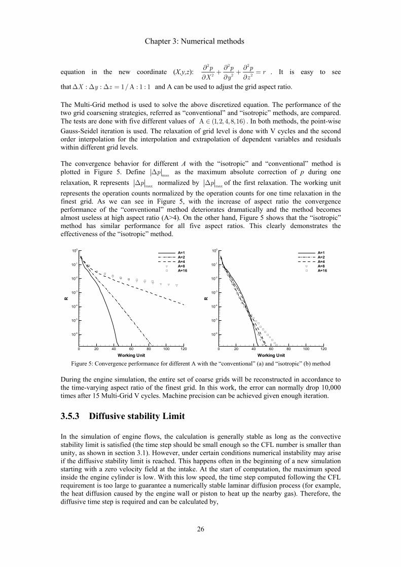
Chapter 3: Numerical methods
26
equation in the new coordinate (X,y,z): 2 2 2
2 2 2
p p p rX y z∂ ∂ ∂+ + =∂ ∂ ∂
. It is easy to see
that : : 1/A : 1 : 1X y z∆ ∆ ∆ = and A can be used to adjust the grid aspect ratio.
The Multi-Grid method is used to solve the above discretized equation. The performance of the two grid coarsening strategies, referred as “conventional” and “isotropic” methods, are compared. The tests are done with five different values of A (1,2, 4, 8,16)∈ . In both methods, the point-wise Gauss-Seidel iteration is used. The relaxation of grid level is done with V cycles and the second order interpolation for the interpolation and extrapolation of dependent variables and residuals within different grid levels.
The convergence behavior for different A with the “isotropic” and “conventional” method is plotted in Figure 5. Define maxp∆ as the maximum absolute correction of p during one relaxation, R represents maxp∆ normalized by maxp∆ of the first relaxation. The working unit represents the operation counts normalized by the operation counts for one time relaxation in the finest grid. As we can see in Figure 5, with the increase of aspect ratio the convergence performance of the “conventional” method deteriorates dramatically and the method becomes almost useless at high aspect ratio (A>4). On the other hand, Figure 5 shows that the “isotropic” method has similar performance for all five aspect ratios. This clearly demonstrates the effectiveness of the “isotropic” method.
Working Unit
R
0 20 40 60 80 100 120
10-6
10-5
10-4
10-3
10-2
10-1
100
A=1A=2A=4A=8A=16
Working Unit
R
0 20 40 60 80 100 120
10-6
10-5
10-4
10-3
10-2
10-1
100
A=1A=2A=4A=8A=16
Figure 5: Convergence performance for different A with the “conventional” (a) and “isotropic” (b) method
During the engine simulation, the entire set of coarse grids will be reconstructed in accordance to the time-varying aspect ratio of the finest grid. In this work, the error can normally drop 10,000 times after 15 Multi-Grid V cycles. Machine precision can be achieved given enough iteration.
3.5.3 Diffusive stability Limit
In the simulation of engine flows, the calculation is generally stable as long as the convective stability limit is satisfied (the time step should be small enough so the CFL number is smaller than unity, as shown in section 3.1). However, under certain conditions numerical instability may arise if the diffusive stability limit is reached. This happens often in the beginning of a new simulation starting with a zero velocity field at the intake. At the start of computation, the maximum speed inside the engine cylinder is low. With this low speed, the time step computed following the CFL requirement is too large to guarantee a numerically stable laminar diffusion process (for example, the heat diffusion caused by the engine wall or piston to heat up the nearby gas). Therefore, the diffusive time step is required and can be calculated by,

Chapter 3: Numerical methods
27
( )2 2 2
max
0.2 min , ,Pr (2 / )D x y zτ
µ ρ∆ = ⋅ ∆ ∆ ∆
⋅ (50)
At the beginning of an intake, the grid distance x∆ in the axial direction of engine cylinder is the smallest since the piston is closest to the engine head. If the diffusive time step is smaller than the convective time step, the diffusive time step is used for advancing the system. It is interesting to note that the diffusive limit can not be reached at the end of compression stroke since the flow at that moment is quite turbulent and thus the convective time step is even smaller than the diffusive time step.
3.6 Features of the in-house LES codes used in this thesis
In this thesis we focus on problems of turbulent reactive flows which are studied by LES method. To do LES, a Computational Fluid Dynamics (CFD) code is written by the author. The code is based on a previously existing in-house code written with the programming language FORTRAN. The code is re-written in the programming language C++ with several improvements and features listed below.
1 The Low Mach number version of the FORTRAN code has been changed from previously full-implicit solver to semi-implicit method. In the full-implicit implementation, at each time step all transport equations including momentum, mass and energy equations are discretized in the future time steps. Since all these equations are coupled, it is computationally heavy to iterate the large system to converge. The full-implicit strategy originates from RANS approach in which large time step is normally used; for steady RANS problem the implicit method can be faster. However, in LES small time step is required to capture the dynamics of small scales. The full-implicit algorithm becomes less efficient and not economical. Therefore, in the new C++ implementation a semi-implicit method is used. This implementation is similar to the traditional fractional step method [56, 57], in which only the continuity equation and the pressure gradient terms in the momentum equations are discretized in future time step. This method results in only a Poisson equation for pressure to be resolve iteratively. With the fractional step method, the transport equations of momentum and scalars are discretized explicitly; appreciable computational effort is therefore reduced. Moreover, it is easy to achieve convergence for the pressure Poisson equation. The machine precision can be reached in the new implementation. While the iteration step is the most computational heavy step in both methods, the total computational time for one time step is greatly reduced in the C++ code than in the FORTRAN code, under the same convergence requirement.
2 The accuracy of discretizing convective terms has been improved: in the new code, the 5th order Weighted Essentially Non-Oscillatory Schemes (WENO) scheme is used. The WENO scheme is suitable for doing LES of the engineering flow problems in the sense of keeping accuracy while achieving better stability. For engineering problem there may exist large gradients in the flow field. The problem is not suitable for the dissipative-free schemes, like the energy conservative scheme, which are designed for flows with weak gradients in the flow field. The simulation is often unstable if those methods are used directly. With traditional upwind scheme the stability can be improved; however, compared to the WENO scheme it is less accurate in the smooth region if the same stencil is used.
3 The support for parallelization is enhanced in the new code. The parallelization is based on domain decomposition. Within one computational domain, the code supports division of computational blocks in all three directions. Suppose that Ix, Iy and Iz are the section number by which the domain is split in the three directions respectively, the domain is divided into Ix×Iy×Iz blocks; each of which can be handled by one computer processor. Furthermore, the code supports multiple computation domains. The domains can interact through one interface.

Chapter 3: Numerical methods
28
The parallel implementation ensures the preservation of accuracy; no accuracy is lost at the boundary between two neighboring blocks. It is necessary to mention that the parallelization has been implemented at each layer of grid within the Multi-Grid method for solving the pressure Poisson equation. This strategy is necessary for the iteration to converge efficiently when the Multi-Grid method is running at parallel mode. While it is relatively easy to implement the parallelization in an explicit method for a hyperbolic problem (such as a fully compressible flow), the parallel implementation in an implicit method for an elliptical or parabolic problem (such as an incompressible or low Mach number flow) requires more consideration, since compared with hyperbolic problem, in elliptical or parabolic problems certain information propagates fast (like the pressure wave in our case). For convergence in parallel computations, each processor should exchange information with all the other processors; this must be done in an efficient way.
4 The structure of the CFD code has been redesigned with the object oriented programming concept by the C++ programming language, which is already used by well-known CFD codes (e.g. OpenFOAM [71]). In the present in-house code, the parallelization and the Multi-Grid method determine the main programming structures, while the grid and boundary condition is implemented in a modular way.
The developed in-house code has been applied for different cases: for example, simulations of turbulent diffusion flames (Paper 8 and 9), partial-premixed flames (paper 10) and also simulations of engine flow and auto-ignition process. In the diffusion flame a mixture fraction equations is solved and in partial premixed flame an additional level-set equation [19, 64] is solved. In this thesis the numerical method is mainly discussed for the IC engine cases. Other numerical details for the flame cases can be seen in the corresponding papers.
3.7 Validation of the LES solver
To validate the numerical solver, an existing engine experiment is simulated. The engine (reported by Boree et al.[72]) has a simple geometry with a rectangular shaped chamber, running at low speed (206 rpm). The intake port is a long planar channel; the flow in this engine can be regarded to be statistically two-dimensional. The rectangular engine is specially designed to investigate the tumble motion in the IC engines. Compared with practical engines, this engine is of simple geometry, thereby providing a suitable test case for validation of simulation models.
Figure 6 : Sketch of the experimental rectangular engine.
The square engine experiment is done by Boree et al.[72, 73]. The engine geometry is sketched in Figure 6, where b=100mm is the width and also the height of the chamber. The piston is moving sinusoidally at ω=206 rpm. t=0 denotes the start of the intake; the piston position is described by Xp, where Xp(t)=b-Vp/ω(1+cos(ωt)). The maximum piston speed is Vp=0.809m/s.
Xp(t)
h
b
piston
Intake Channel
b
zx
y
Compression stroke Intake stroke

Chapter 3: Numerical methods
29
The intake system is a long flat channel with a height of the intake channel h=10mm and length of the intake channel L=300mm. Considering the simple geometry and condition of the engine, this is a good validation case for the numerical method. A previous LES study of this engine has been reported in [74].
The computational domain in this study consists of both the rectangular engine chamber and the intake channel. The engine chamber is described with moving grid with 1283 cells, whereas the intake channel is simulated with fixed grid 128×72×72 in the x, y, z directions, respectively. The two domains are interconnected using interpolations for scalars and vector at the interface of the domains. By doing so, the inflow condition, i.e. the flow at the exit of the intake channel where the gas enters to the combustor, is simulated. The inflow boundary condition for the intake channel is not influential to the flow field developed in the intake channel, therefore a simple laminar plug flow is assumed at the inlet of the intake channel. Further details can be seen in paper 1.
With the current grid resolution, the averaged y+ at middle intake stroke (i.e. when the intake stream has highest speed) is around 6; this y+ value is averaged over all the walls of the rectangular chamber. Since the engine is running in motor condition, the spatial density ratio inside the engine chamber is small, therefore only the predictor step is needed. The mean and root-mean-square (rms) velocity have been computed from the experiments using 120 cycles of 2D PIV velocity data. Since the computation is rather expansive, 20 simulated cycles have been performed. The simulation starts with initial random turbulence field generated assuming isotropic turbulence [75, 76] insider the chamber. The wall temperature is set as 300K. The residual gas in the chamber is set as 290K; the gas coming from the intake channel is set as 280K.
3.7.1 Instantaneous vorticity field
Figure 7 shows the instantaneous vorticity fields from LES and experiment at the intake stroke. The vorticity components along z-axis at different cycles and piston positions are shown in the figure. The experimental z-vorticity is calculated from PIV results. The vorticity field from both experiment and LES looks qualitatively similar. In these plots, strong vortices can be seen developed after the intake channel. The region of high level vorticity follows the tumble motion which is formed from the intake stream. The tumble flow is deflected by the piston that moves away from the exit plane of the intake channel first, and then returns after reaching the bottom dead center. On the edge of tumble flow, the gradient in the flow velocity is high, which leads to generation of intensive turbulent eddies.

Chapter 3: Numerical methods
30
Figure 7: Instantaneous vorticity fields during intake (ωz denotes vorticity component along the z-axis). From left to right: Xp=60, 60, and 80 mm; First row: Exp; Second row: LES.
3.7.2 Mean tumble flow
To illustrate the tumble flow motion further, Figure 8 shows the mean velocity vector plots at the intake and compression stroke. The experimental mean velocity is averaged from 120 cycles of data while LES does only 20 cycles due to limitation of computation power. The tumble motion is well represented by the major counter-clockwise rotating structures in all plots. Both the center position and evolution of the mean tumble motion predicted by LES are comparable to the experimental results. In intake stroke (Xp=40 and 60mm) there exists a clockwise rotating flow structure in the low right corner. This corner recirculation zone is nearly invisible in the compression stroke (Xp=60mm), however, the center counter-clockwise recirculation zone retains in the compression stroke. As shown in Figure 7 high level vortices are clustered in the corner recirculation zone, where the local flow can be highly turbulent and with fine structures.
Xp=60 mm Xp=80 mm Xp=60 mm
LES
Exp.

Chapter 3: Numerical methods
31
Comparison of the mean and rms velocity profiles are further discussed in paper 1, where it is shown that fairly satisfactory comparison between the LES results and the experiments is obtained with the current LES solver. With this validation the LES solver is applied to simulations of several IC engines with realistic geometry.
Figure 8: Mean velocity vector field in the mid-z plane from experiments (upper row) and LES (lower row). From
left to right: Xp=40 mm (intake), 60 mm (intake), 60 mm (compression) mm.
Exp.
LES
x
y
0 0.2 0.40
0.2
0.4
0.6
0.8
15 m/s
x
y
0 0.2 0.40
0.2
0.4
0.6
0.8
15 m/s
x
y
0 0.2 0.4 0.60
0.2
0.4
0.6
0.8
1x
y
0 0.2 0.4 0.60
0.2
0.4
0.6
0.8
1
Xp=60 mm Compression
Xp=60 mm Intake
Xp=40 mm Intake
x
y
0 0.2 0.4 0.60
0.2
0.4
0.6
0.8
1x
y
0 0.2 0.4 0.60
0.2
0.4
0.6
0.8
1

Chapter 4: Quantification methods
32
4 Quantification of in-cylinder turbulence and combustion
LES generates three dimensional, time dependent data that describe the instantaneous flow structures, temperature, pressure and composition field. These data are however of little use without proper post-processing. Quantify turbulence and the combustion process is not a trivial task. It is conventional to quantify turbulence using ensemble average of the instantaneous cycle resolved flow [77]. This, however, would filter out many small scale details of turbulence. In the following several methods of quantification of in-cylinder turbulence and the combustion process are discussed.
4.1 Velocity vector field, streamlines, and vorticity field
It is typical to visualize the flow field using two dimensional velocity vectors. The direction and magnitude in the velocity vector field can be well represented. Large scale recirculation zones can be identified from the velocity field. However, small scale eddies are often difficult to visualize without proper choosing of the zoom window. Three dimensional velocity vectors are often difficult to visualize, and also very fine grid resolution can often lead to too dense vector field. Figure 9 shows a typical velocity vector field in a cross section of a HCCI engine to be discussed in section 5.1.
According to Tennekes and Lumley [78], turbulence is viewed as a tangle of vortex filaments and the physics of turbulence can be much explained using the vortex dynamics. The concept of a turbulence eddy is sometimes meant by a vortex that has locally spatial coherent structures [49]. Although the concept of vortex is widely used in fluid mechanics, a universally accepted definition of a vortex is still lacking. Lugt [79] defines a vortex as a ‘multitude of material particles rotating around a common center’. Jeong and Hussain [80] have reviewed different approaches of visualizing vortex cores, i.e. the rotational structures in turbulent flows. These include commonly used intuitive methods – streamlines, isosurface of vorticity and pressure minimum.
Streamlines can be used to visualize the flow directions. At each point of the streamlines the tangential direction is the velocity vector direction. Streamlines can represent rotational structures not only for large scales (such as the swirl motion) but also for small scales. Streamlines can also represent three dimensional structures. In Figure 9 the velocity field is shown using streamlines (in addition to the velocity vectors). Compared with the velocity vector field, the large scale swirl motion in the cylinder is shown clearer with the streamlines.
Vorticity vector is defined mathematically as the curl of the fluid velocity. Physically, it corresponds to the circulation per unit area at a point in a fluid flow field, thus the magnitude of vorticity denotes the strength of the rotation motion. The direction of vorticity vector is along the axis of the rotation. In Figure 9 the flow field is also shown using the vorticity component that is normal to the shown cross section. As seen, compared to the velocity vectors and streamlines, the vorticity contours show the small rotational structures clearer. The low left part of the flow field exhibits more rotational structures.
The third method to visualize rotational structures is the minimum of hydrodynamic pressure. As shown in Figure 15, later in section 5.1.2, at the centre of a large scale swirl flow, the hydrodynamic pressure is low to generate a pressure gradient to balance the centrifugal force induced by the swirl motion.

Chapter 4: Quantification methods
33
Figure 9: Visualization of instantaneous flow field in a cross section using different methods; (a), velocity vectors; (b) 3D streamlines; (c) contours of vorticity component normal to the cross section; (d) λ2 contours, the positive
region is blanked in white.
4.2 The λ2 method
It was argued that the use of streamlines, vorticity and pressure minimum is sometimes inadequate [80]. For example, a well-defined pressure minimum can exist in an unsteady irrotational flow. The topology of streamlines is not Galilean invariant, i.e., in different reference coordinates the streamlines are different. The isosurface of vorticity is more often used and fairly successful to identify rotational structures; however, this approach may not always be satisfactory. For example, in a laminar wall boundary layer, high velocity gradient exists with very high vorticity at the wall; yet, the flow does not have rotational structures. A so-called λ2 method has been developed to identify the rotational cores [80]. Here λ2 is the median of the three eigenvalues of 2 2
ij ji ij jiS S S+Ω = +Ω Ω , where ijS and ijΩ are the symmetric part and anti-symmetric part of the velocity gradient tensor:
X Y
Z
30
60 CAD
m/s
(a) (b)
(c) (d)

Chapter 4: Quantification methods
34
1 1,2 2
j ji iij ij
j i j i
u uu uS
x x x x
∂ ∂∂ ∂ = + Ω = − ∂ ∂ ∂ ∂
They are also known as the rate of strain tensor and rate of rotation tensor, respectively. Since 2 2S + Ω is symmetric, it has real eigenvalues only. Denote 1 2, λ λ and 3λ the three eigenvalues
and 1 2 3λ λ λ≥ ≥ . The rotational core may be defined as the connected flow region with two negative eigenvalues, i.e. 2 0λ < . This so-called 2λ -method has been shown to properly represent the complex topology and geometry of vortex cores. It is Galilean invariant. In many test cases the 2λ -method was shown to be superior to the intuitive methods such as the pressure minimum, the streamlines and the vorticity isosurfaces. In Figure 9, the contours of negative λ2 are shown. As seen the λ2 vortex cores are, to certain extent, similar to the isocontours of vorticity. It should be pointed out that most of these methods, except the vorticity isosurface method, show the topology of the rotational structures only. For simple rotational core structures, e.g. the Lamb vortex, the λ2 method can be rather precise; however, for complex vortex structures in turbulent flows, the region of 2 0λ < can be rather messy. In order to show clearer vortex core structures, one sometimes uses a lower negative 2λ isofuraces to identify the vortices. In Figure 10 the instantaneous flow structures are visualized using both the 3-D streamlines and the 2λ -method. As seen, the 2λ -method illustrates more details about the rotational filaments in the cylinder.
Figure 10: Instantaneous flow structures and temperature field in a HCCI engine with square-bowl shaped piston, visualized using 3D streamlines, λ2-method, and contours of temperature field. More details about the engine is
given in paper 7.
streamlines λ2-isosurface

Chapter 4: Quantification methods
35
4.3 Statistical description of in-cylinder flows
Ensemble average approach
It is conventional to apply ensemble average to obtain the mean and fluctuations of a flow property such as velocity, temperature or species mass fractions. Ensemble average requires data from many cycles. The ensemble average method is often used in engine experiments since it is rather easy to gather data from different cycles when the engine is continuously running. For LES, the ensemble approach can be quite difficult due to the heavy computational costs for multi-cycle simulations. In this work the ensemble average approach is used only in the simple engine case with rectangular shaped chamber (section 3.7), in which twenty cycles of simulations have been performed. This small amount of sampling may not be sufficient for computing accurately turbulence fluctuation; however, for the mean values twenty cycles can be rather fine.
Spatial filtering approach
Another way to quantify the turbulence is by a spatial filtering method.
1 1 2 2 3 3 1 2 3 1 2 3( , , ; ) ( , , )i iu G x x x x x x u x x x dx dx dx′ ′ ′ ′ ′ ′ ′ ′ ′= − − − ∆∫∫∫
where ( 1,2, 3)iu i = are the LES resolved velocity components in Cartesian coordinates ( 1,2, 3)ix i = directions, respectively. G is a Gaussian filter function with filter width .∆
iu are the velocity filtered on a large length scale .∆ When ∆ is chosen as the turbulent integral scale, one obtains a filtered ‘smooth’ velocity field that contains energy of the integral scales only.
Accordingly, one may define a quantity u ′ as follows:
( ) ( ) ( )1/2
2 2 21 21 2 3 3
1 ˆ3
V
u u u u u u u dVV
′ = − + − + − ∫ ,
where V is the volume of the entire cylinder. The overall turbulent fluctuation is kept in the quantity .u ′ It is the root-mean-square of LES resolved velocity subtracted by the filtered velocity, thus it is a good measure of the energy level of the small eddies (smaller than integral scales but larger than the LES resolved scales).
During most period of the engine cycle, the size of filter ∆ may be chosen as one tenth of the cylinder diameter. This filter size is the same all three directions. However when the piston moves close to the engine head, the filter in the direction of piston moving should be adjusted to be the minimum between this value and the distance from the piston top wall to the cylinder head. The adjustment allows for the continuous calculation of u ′ through the whole cycle.
With the filter method, only one cycle simulation is needed. u ′ can be computed from the instantaneously velocity field.
Pressure trace, heat release rate, and normalized cumulative heat release
In engine experiments it is typical and convenient to measure the pressure inside the cylinder at a selected point [81, 82]. The pressure variation in space is generally small compared with the value of the pressure therefore the in-cylinder pressure can be represented by single value. This pressure

Chapter 4: Quantification methods
36
corresponds to the thermodynamic pressure (P) discussed in Chapter 2. This is, however, not the case when ‘knocking’ occurs [77].
From the in-cylinder pressure one can derive the heat release rate and the total heat release that denote the ignition event. In LES the heat release rate can be readily computed from the rate of the reaction progress variable, whereas the total heat release can be computed from the reaction progress variable itself.

Chapter 5: Results and discussions
37
5 Results and discussions
The turbulent flow inside IC engines is vital to the engine performance. While general understanding about in-cylinder flow is available based on many experimental and computational works as summarized in the book of Heywood [77], and the recent review by Miles [36], the flow details, such as the turbulent eddy structures and instantaneous flow field in the cylinder, are less reported. Large eddy simulation, which is capable of capturing the energetic turbulent eddies, brings an opportunity to provide detailed knowledge about the engine in-cylinder flow. In this chapter LES results about the engine in-cylinder flows, heat transfer and their effect on HCCI auto-ignition are discussed to highlight the basic characteristics of the physical and chemical process in HCCI engines. Further details are given in the attached papers.
Several engine configurations are studied in this thesis, including a rectangular shape engine that has been discussed in chapter 3, and more practical engine geometries that are studied experimentally in the Combustion Engine Laboratory at Lund University. All the studied engines are operated in four-stroke mode, i.e. an engine cycle is made up of the intake, compression, expansion and exhaustion strokes. In the following the in-cylinder flow structures from LES in the different strokes of the engine cycle are presented, followed by discussions of the evolution of turbulence and temperature inhomogeneity. Finally, the effect combustor geometry on the auto-ignition in HCCI engines is discussed.
5.1 Instantaneous flow structures and temperature stratification
The engine discussed here is based on an existing HCCI single cylinder engine [83] studied at the Combustion Engine Laboratory at Lund University. The engine head and piston are made flat to facilitate laser diagnostics; the engine chamber is of cylindrical shape. The engine is operated at speed of 1200 rpm. Other details can be seen in paper 5.
Several grid resolutions have been tested in the LES study. The following results are based on the computational grid with 2563 cells. With this fine resolution the non-dimensional length of the first near-wall grid (y+) can reach an average value (over the entire cycle) about 5, thereby allowing for a more accurate treatment of the wall boundary layer. The simulation starts from intake stroke where the piston is at the top dead center (TDC) (denoted as 0 crank angle degree, CAD in the subsequent figures). To illustrate the development of flow and temperature stratification, the simulation starts from zero velocity field and homogenous temperature field (T=60oC or 333K) for the piston position at the TDC. The inflow and wall temperatures are estimated from typical engine experiments. The temperature of the fresh intake gas is set to be 30oC (303K). The piston wall temperature is set to be 230oC (503 K) to mimic the quartz piston (Paper 4) while the temperature of the cylinder wall is set to be 130oC (403K) since the wall is cooled more effectively than that for the quartz piston. There are two intake valves and two exhaustion valves located on the engine head. The opening valves are modeled by annular inlets/outlets as discussed in section 2.5. The two intake valves are assumed to open simultaneously at 0 CAD (piston at TDC).
The flow characteristics are quite different during different stages of engine cycle. In the following the flow structures in the four strokes of the engine cycle is discussed separately, starting from intake stroke.

Chapter 5: Results and discussions
38
5.1.1 Intake stroke
The instantaneous vortex structures at an early intake stroke (e.g. 30 CAD) are visualized in Figure 11a. For convenience, the engine is shown “upside down”– the piston is on the top of the figure whereas the intake inflow is on the bottom plane of the figures. The engine head is shown on the bottom of the figure (y-z plane) together with the x-z plane crossing the center of the cylinder to illustrate the three dimensional flow structures. Figure 11b shows the temperature field on the same planes.
Figure 11: The 3D vortex structures (green filaments) visualized using lambda-2 method (a) and the temperature field (b) on two planes at intake 30 CAD.
As shown in Figure 11 the temperature field at the early intake stroke can be divided into four regions, 1) the residual gas region, 2) the fresh gas region, 3) the near wall boundary layer, and 4) the mixing region. The fresh cold gas (303K) is inhaled into the cylinder through the two annular intake ports. Random vortex structures are seen in the proximity of the intake ports. The observed vortex structures are generated mainly from the shear layer downstream of one of the intake ports that has higher flow speed due to the difference in the geometry of the intake ports.
Near the piston wall (shown as the top of the vertical plane), high temperature gas spots can be seen rolling away from the piston wall. At the centers of rolling structures, one can see vortex ‘pipes’. This indicates that the hot spots are transported by the rolling vortex flows.
From this figure it is clear that at the initial intake stroke the production of turbulence is mainly due to the high-speed flow in the shear-layer downstream of the intake ports whereas the generation of temperature stratification is mainly due to the flow in the boundary layer, and to some extent due to the mixing of the intake gas with the residual gas from the previous cycle. In section 5.3 and paper 5 the statistics of the temperature stratification is further discussed.
(a) (b) Cylinder head
piston

Chapter 5: Results and discussions
39
Figure 12: The temperature field ( T: left column) and projected vorticity field ( ω⊥ : right column) at 60 CAD at
different cutting planes. (a), x-z-plane; (b) x-y plane; (c) y-z plane. The vorticity component normal to the plotting plane is shown, i.e. ωy at x-z plane, ωz at x-y plane and ωx at z-y plane.
The temperature field and projected vorticity field at a later intake stroke (i.e. 60 CAD) are plotted in Figure 12. The shown planes are x-y and x-z planes crossing the cylinder axis, as well as the y-z plane in the middle of the cylinder. At this moment, the temperature field is more irregular illustrating a random turbulent flow nature. The four temperature zones shown in the early moment (30 CAD) become less distinguishable. As fresh gas is inhaled into the cylinder, the region for the residual gas decreases. The mixing between the residual gas and the fresh intake gas is enhanced due to developed turbulence (as indicated by the vorticity contours).
It is interesting to note that there is strong correlation between the vorticity field and the temperature field. In places where the vorticity level is low (in absolute value), the temperature is also more uniform (e.g. the white zone in the temperature field). Near the top wall in x-z and x-y planes, fine rolling structures can be seen in the temperature field. In those region, the vorticity field suggests existence of rotational flows. The process of turbulence enhanced heat transfer is clearly demonstrated by the fine rolling structures observed near the boundary layer.
(a)
(b)
(c)
ω⊥

Chapter 5: Results and discussions
40
Figure 13: The vortex structures and the temperature field at 90 CAD. For better viewing of vortex structures, the cylinder is split into two parts: (a) near cylinder wall region and (b) the rest inner region. The flow near one of the
inlets is shown in c. The temperature field is shown in d.
The instantaneous flow structures at the middle intake stroke (90 CAD) are shown in Figure 13. At this CAD, the gas is inhaled into the cylinder at the highest velocity. The flow becomes highly turbulent due to the high speed intake flow. Figure 13b shows that a large number of irregular vortex structures are clustered at the downstream of the intake ports. The detailed flow structure around one intake port is zoomed in the Figure 13c in which the 3D streamlines are also plotted. The flow swirl and tumble motions are seen from the streamlines in the figure. The high speed flow stream is first directed by the cylinder wall to turn upward and then deflected by the piston. Figure 13a shows that near the cylinder wall there exist many vortex tubes which are aligned perpendicular to the flow stream.
The temperature field at 90 CAD is shown in Figure 13d. The cold gas resides mainly in the low part of the cylinder - near the entrance of the intake stream; substantial mixing takes place in other regions of the cylinder as a consequence of the strong turbulence developed in the flow field. The near wall heat transfer is also enhanced by the turbulence. There is a high temperature region near the left part of the upper region. This region is a low-speed recirculation corner where the gas is heated up by the nearby hot wall.
(a) (b)
(d) (c)

Chapter 5: Results and discussions
41
Figure 14: Vortex structures and the temperature field at the end of intake stroke (i.e. 180 CAD). The cylinder is
split to outer near wall region (a,b) and the inner region (c). The temperature field is plotted together with 3d streamlines in (d).
The vortex and temperature field at the end of the intake stroke (180 CAD) is shown in Figure 14. Near the end of the intake stroke, the intake flow slows down; therefore less kinetic energy is brought into the cylinder to feed the turbulence production. The previously developed turbulence starts decaying. Figure 14 shows that the vortex is distributed more homogenously over the cylinder than in the earlier intake stroke. The inner vortexes show a tendency to align preferentially in the cylinder axis direction while the vortex tubes in the near wall region are perpendicular to the axis direction. The tumbling and swirling motions are visualized by the 3D streamlines in Figure 14d in which the temperature field is also plotted. The temperature field is shown very stratified; the hot gas stays close to the piston (top of the figure) while cold gas stays close to the intake ports (bottom of the figure).
5.1.2 Compression stroke
Flow structures
In the compression stroke all intake valves are closed. The evolution of the flow field in a closed system is rather different from that in the intake stroke. Figure 15 shows the instantaneous hydrodynamic pressure fields at four consecutive CAD during compression. In these figures the
(a) (b)
(c) (d)

Chapter 5: Results and discussions
42
pressure iso-contour lines are plotted in both y-z plane and x-z plane. A 3D iso-surface of a low pressure is plotted in each pictures; the region with pressure lower than this value is inside the iso-surface. 3D instantaneous streamlines are also plotted in the figures.
Figure 15: Isocontours of instantaneous hydrodynamic pressure at different CAD in the compression stroke: (a) CAD=300; (b) CAD=310; (c) CAD=320; (d) CAD=340. The low pressure centre is shown by the 3-D iso-surface
of hydrodynamic pressure.
In the compression stroke, the swirling and tumbling motions inherited from intake stroke determine the large scale flow structure inside the cylinder. The low pressure region is seen to locate at the center of the large scale rotational motion. At 300 CAD, Figure 15a, the pressure in the y-z plane decreases monotonically from the outer to the inner region. The low pressure region in this plane is of an ellipse shape, with its center of which locates off the cylinder axis. This is a result of the swirling motion. As discussed in Section 4.3, the iso-surface of the minimal hydrodynamic pressure, together with the 3D streamlines, indicates the center core of the rotational motion. As seen in the figure, the axis of center core is not vertical. The tilting of the low pressure core zone is a result of tumble motion.
It can be seen that the piston motion that compresses the in-cylinder flow has an effect on the low pressure core. Indeed the low pressure core zone breaks down near the piston. In this region, the downward movement of the piston interacts directly with upper part of the tilted rotational core. As the piston moves further down to compress the in-cylinder gas, less space is left for the tumble motion to sustain. As the compression progresses further, the low pressure core breaks up further, as showed in Figure 15b-Figure 15d. This indicates the loss of well-organized large scale swirl motion.
(a) (b)
(c) (d)

Chapter 5: Results and discussions
43
Figure 16: Temporal evolution of the rotational direction of the low pressure core (clockwise) and the flow swirl
motion (counter-clockwise, indicated by the streamlines).
It is interesting to note that the axis of the low pressure core (the white dashed line in Figure 16) rotates slowly in the clockwise direction as the piston moves from 300 CAD to 310 CAD. This slow rotational motion is opposite to the flow swirling direction that is counter-clockwise. This is shown in Figure 16, where the 3-D field in Figure 15 is projected into the y-z plane.
Temperature field and hot zone
Figure 17 shows the temperature field at two CADs in the compression stroke (300 and 320 CAD). During compression stroke, the averaged gas temperature increases due to compression of the charge. At late compression stroke, the wall temperature is lower than the gas temperature in the cylinder. In Figure 17, the low temperature zones (<470K at 300CAD, <550K at 320CAD) are shown as the grey zone near the wall. The iso-surfaces of a high temperature (600K at 300 CAD, 700K at 320 CAD) are also plotted in the figure; regions with higher temperature are wrapped inside the iso-surfaces.
It is interesting to note that the hotter gas is not distributed homogenously in the y-z plane. This will lead to the inhomogeneous onset of auto-ignition in the cylinder. The hotter pockets will auto-ignite earlier than the colder pockets. This phenomenon is consistent with previous experiments reported in [9, 12, 17].

Chapter 5: Results and discussions
44
Figure 17: The temperature field during compression stroke: (a) 300 CAD, (b) 320 CAD.
5.1.3 Expansion stroke
Figure 18 shows the flow and temperature fields at 400 CAD. In this case the engine has been set to be motored run, i.e. without auto-ignition of the charge. This is to examine the development of the temperature stratification and flow structures.
As seen in Figure 18, the low pressure core stands vertically near the center. The stream lines also indicate that swirling motion remains in the cylinder whereas the tumble flow is weak. The gas temperature is higher than the wall temperature. The gas becomes colder during expansion.
Figure 18: The flow and temperature fields at the expansion stroke (400 CAD) for a motored run case.
5.2 Evolution of turbulence
The results shown in the previous section illustrate the potential of LES in capturing fine details of the flow and temperature field. The discussions have been mainly based on instantaneous fields. It was shown that the characteristic of large scale flow motion can be quite different at different strokes of one engine cycle. At the intake stroke, the flow is dominated by the high speed intake
(a) (b)

Chapter 5: Results and discussions
45
flow which brought into the cylinder with kinetic energy. The high speed stream becomes quickly turbulent and turbulence spreads quickly to the other part of engine domain. After the intake valve is closed, the turbulence is maintained by the kinetic energy saved in the previous flow and by the piston motion.
As discussed in section 4.3, the level of turbulence may also be quantified using spatial filtered velocity fluctuations (u ′ ). As an example, the evolution of u ′ for the case discussed in the previous section (5.1) is plotted in Figure 19. The value of u ′ increases rapidly first in the early intake stroke (0<CAD<50), and then it decreases in the later intake stroke and earlier compression stroke (50<CAD<270). It increases again in the later compression stroke (270<CAD<330). Thereafter, u ′ decreases monotonically (CAD>330).
Figure 19: Evolution of u ′ in a four stroke engine.
The increase of u ′ in the early intake (0<CAD<50) can be explained by the turbulence production from the intake stream, starting from a laminar field. The high speed jet enters into relatively small volume of cylinder during early intake, thus turbulence reaches to maximum level very fast. The decay of u ′ during later intake stroke is due to the increased cylinder volume thus lower shear-stress (less disturbance) to the flow. The decreasing tendency of u ′ continues until the middle compression stroke (270 CAD). In the compression stroke, all the valves are closed, turbulence decays due to viscous damping.
It is interesting to observe the increase of u ′ during the later compression stroke. This may be explained by the enhanced turbulence production due to compression. In [36] this phenomenon is explained by examining the equation of turbulence kinetic energy – the k-equation. Assuming spatially uniform density, the turbulence production term in k equation comprises the isotropic and
anisotropic parts, the isotropic part can be written as 2 ( )3k U− ∇ ⋅ , where U is the mean velocity
vector. From the continuity equation it appears that (1/ )( / )U tρ ρ∇ ⋅ =− ∂ ∂ , during compression this term is negative. Thus, the turbulence production contributed by this isotropic part is positive, thereby it leads to an increase of turbulence kinetic energy. The process can be interpreted physically: that compression brings closer the previous distant turbulence eddies, thus increases the shear-stress in the flow to force the flow to be more energetic.
In the late compression stroke (330 CAD), turbulence decays. Close to the top dead center, the compression related / tρ∂ ∂ term is rather small, thus turbulence decay is the dominant process. Turbulence production is not enough to balance the viscous damping. This trend is maintained in the expansion stroke where the turbulent production becomes negative.
CAD
u' ∆
0 90 180 270 360 450 5400
2
4
6
8
10
u'∆

Chapter 5: Results and discussions
46
5.3 Evolution of temperature inhomogeneity
The combustion characteristics in HCCI engines can be greatly affected by the temperature inhomogeneity prior to the onset of auto-ignition. The evolution of temperature field is affected greatly by the process of turbulent heat transfer, as already shown in the instantaneous plots in sections 5.1.
For temperature inhomogeneity to form, the first requirement is the existence of temperature difference between different components of the engine system. In addition to the intake gas temperature, temperatures of the residual gas from the previous cycle, the engine cylinder wall, and the piston wall can cause temperature stratification in the cylinder. The piston wall temperature is different from the cylinder wall temperature due to the fact that quartz piston is used in engine experiment and the cooling of the piston is different from that of cylinder; the quartz piston is typically hotter than the metal wall,
In addition to temperature difference, the turbulent flow is a factor that controls the heat transfer process in the cylinder. There are two roles played by turbulence in the generation of inhomogeneity in temperature field. Near the engine walls, turbulence helps heating up or cooling down the gas thus increases temperature inhomogeneity. Inside the engine cylinder, turbulence helps decreasing any existing inhomogeneity by enhanced mixing.
To investigate the development of turbulence and temperature stratification in the intake stroke and the compression stroke, several cases have been simulated. The system considered is the same cylindrical engine with flat piston as in section 5.1. Details of initial and boundary conditions for the test cases are given in Table 2 and Table 3.
Table 2: Case description for the simulation of intake phase (0≤CAD≤180).
Cases Initial field Wall temperature [K] CC0 Flow and T field from CI0 at CAD=180 Piston: 503, other: 403 CC1 Same as CC0 Adiabatic CC2 Same as CC0 403 CC3 Flow field same as CC0, T= <T> Same as CC0
Table 3: Case description for the simulation of compression & expansion phase (180≤CAD≤300).
Four simulations have been carried out for the intake stroke (0≤CAD≤180) in Table 2. CI0 is the baseline case, with the temperature of residual gas is slightly (30K) higher than the fresh gas, and the piston wall temperature 100 K higher than the cylinder wall temperature. The baseline case is the same as in section 5.1, in which several instantaneous temperatures are plotted. CI1 is a case with an adiabatic wall and an initial residual gas temperature T=700K. In CI2, the temperature of the residual gas is set to be the same as the intake fresh gas, and the temperature on wall and the piston are the same, 100 K higher than the fresh gas. CI3 has the same initial condition as CI2 and the same wall condition as that of the baseline case CI0.
For the compression stroke of the engine cycle, four cases have also been simulated for 180≤CAD≤300, as seen in Table 3. The baseline case CC0 is a continuation of the baseline case CI0 of the intake phase simulation. Similar to CI1, CC1 is aimed at investigating the effect of adiabatic wall; CC2 is designated to illustrate the piston wall heat transfer; and finally CC3 is simulated to study the preservation of the initial temperature stratification in turbulent flows. In
Cases Residual gas temperature [K] Wall temperature [K] CI0 333 Piston: 503, other: 403 CI1 700 Adiabatic CI2 303 403 CI3 303 The same as CI0

Chapter 5: Results and discussions
47
CC3, the initial flow field is taken as that of CI0 at 180 CAD; the temperature field is set to be a constant, equal to the volume averaged temperature over the entire cylinder of case CI0 at CAD 180.
5.3.1 Intake stroke
To quantify the temperature stratification, we may examine the Probability Density Function (PDF) of the temperature distribution in the cylinder at a given instant or crank angle. Figure 20 shows the temperature PDF for four different test cases listed in Table 2 for the intake stroke.
Figure 20: The temperature PDF at four different intake instants (30, 45, 90, 180 CAD). (a) Case CI0; (b) Case
CI1; (c) Case CI2; (d) Case CI3.
For the baseline case, CI0 (Figure 20a), the temperature PDFs at CAD 30 and 45 (logarithm plot) show several peaks. This is due to the large scale hot spots, as already shown in Figure 20b. The PDF peak at T=303K is due to the intake fresh gas; the peak at T=333K is due to the residual gas remained in the cylinder from a previous cycle. These two peaks are highest in the first two crank angles shown in the figure.
In Figure 20a the peak of PDF near T=500K is due to hot spots derived from the hot piston wall that has a temperature of 503K, and the PDF peak at T=400K is due to hot spot formed near the cylinder walls which is set to be 403K, see Table 2. In between the peaks at 400K and 500K there are several PDF peaks which are corresponding to hot spots formed near the piston at earlier times. In the region between T=360K and 390K there are also several peaks found in the PDF profile;
T[K]
PD
F
Log(
PD
F)
300 350 400 450 5000
0.05
0.1
0.15
10-4
10-3
10-2
10-1
CAD=30(log)CAD=45(log)CAD=90CAD=180
T[K]
PD
F
Log(
PD
F)
300 320 340 360 380 4000
0.05
0.1
0.15
10-4
10-3
10-2
10-1
CAD=30(log)CAD=45(log)CAD=90CAD=180
T[K]
PD
F
Log(
PD
F)
300 350 400 450 5000
0.05
0.1
0.15
10-4
10-3
10-2
10-1
CAD=30(log)CAD=45(log)CAD=90CAD=180
T[K]
PD
F
Log(
PD
F)
300 350 400 450 500 550 600 650 7000
0.05
0.1
0.15
10-4
10-3
10-2
10-1
CAD=30(log)CAD=45(log)CAD=90CAD=180
(a)
(c) (d)
(b)

Chapter 5: Results and discussions
48
they are corresponding to hot spots found near the cylinder walls. These hot spots have cooled down a little as they are transported away from the wall by large vortex structures. Similar PDF peaks are found at CAD 30 and 45 for the cases CI2 and CI3, where the wall temperature, residual gas temperature and/or the intake gas temperature are different.
To verify that the PDF peaks at the earlier intake stroke are formed from wall heat transfer we have simulated a case with adiabatic wall, Case CI1. Indeed, there are no multiple peaks in the PDF profiles (Figure 20b). The PDF has two peaks found at the minimal and maximal temperature in the field. The peak at T=700K is obviously due to the remaining residual gas in the cylinder and the peak at T=300K is due to the intake gas which was set to be 303K (30oC,Table 2). It appears that these hot spot peaks disappear at later stage of the intake stroke, e.g., 90 and 180 CAD. At these crank angles stronger turbulence is developed and it tends to disrupt large hot pocket thus smooth the temperature field.
The effect of hot residual gas on the temperature stratification can be revealed by further examining in Figure 20b. The PDF at 180 CAD in case CI1 shows temperature distribution up to 440K. It is worth to note that turbulence, in this case, plays only the role of mixing to smear the temperature inhomogeneity brought in by the intake cold gas. The PDF results should be quite similar (linearly proportional) if the residual or intake gas has other temperature value.
The wall heating plays an important role in the development of temperature stratification. The PDF peak is shifted to higher temperature as the crank angle increases from 90 to 180, owing to wall heating. The PDFs show two peaks at 90 CAD: the right peak represents the wall heated gas while the leftmost peak represents the newly inhaled cold fresh gas. At this moment, the fresh gas enters the cylinder with quite high speed. It seems too fast for turbulence to mix. At the end of intake stroke (180 CAD), the intake stream slows down to zero velocity, thus the newly inhaled gas is easy to mix by the turbulence, leading to the disappearance of a PDF peak representing the inhaled fresh gas. Instead, this peak moves right to merge with the other high temperature peaks.
Figure 21: Comparison of temperature PDF for case CI1, CI2 and CI3 at the end of intake (180 CAD)
Figure 21 shows the comparison of temperature PDF for case CI1, CI2 and CI3 at the end of intake stroke (180 CAD). Except the obvious wider temperature scattering for case with hot piston (up to 500K in case CI3 than 400K in case CI2), the PDF curve within 300-400K are quite similar for case CI2 and CI3. This indicates that the hot piston has little effect on the temperature field during intake. Figure 21 also shows that the hot residual gas (700K) leads to a temperature distribution comparable to wall heating effect.
T[K]
PD
F
300 4000
0.03
0.06 CAD=180(Resid)CAD=180(Wall)CAD=180(Hot Piston)

Chapter 5: Results and discussions
49
5.3.2 Compression stroke
Figure 22: The temperature PDF during compression stroke. (a) CAD 240; (b) CAD 300; (c) CAD 330; (d) CAD
360.
The PDF of temperature during the compression stroke is shown in Figure 22. The baseline case CC0 differs from case CC2 by a higher temperature in the piston wall, which leads to a higher maximum temperature in the baseline case. The PDF profiles for these two cases are similar in the early compression instants (240 and 300 CAD). However, significant difference shows up in the late compression stroke (330 and 360 CAD). Comparing with the baseline case that has a hot piston, the PDF profile in cases CC2 shows narrow distribution around a high temperature. The temperature field spreads wider in the baseline case. This difference at the late compression stroke plays a significant role in the onset of auto-ignition kernel, since the ignition delay time is very sensitive to the initial temperature prior to ignition. The fact that the piston heating becomes important in the late compression stroke is due to the enhanced heat transfer by the turbulence eddies generated near the piston wall, as already discussed in section 5.1.2.
For the adiabatic wall case CC1, the PDF profile is narrower than case CC2 with non-adiabatic wall, showing the important mechanism of increasing temperature stratification due to turbulence enhanced wall heat transfer. In case CC1, the temperature field is determined by the balance of two effects: the compression and the turbulent mixing. It is worth to note that pure compression leads to increased temperature inhomogeneity, since not only the minimum and maximum temperature in the field but also the difference between them will increase with compression. The turbulence mixing, on the other hand, decreases temperature inhomogeneity by smearing out any existing difference in the field. For case CC1, the temperature PDFs at different compression
TP
DF
450 500 550 6000
0.01
0.02
0.03
0.04
0.05CC0CC1CC2CC3
T
PD
F
350 400 450 5000
0.01
0.02
0.03
0.04
0.05CC0CC1CC2CC3
T
PD
F
650 700 750 8000
0.01
0.02
0.03
0.04
0.05 CC0CC1CC2CC3
T
PD
F
700 750 800 8500
0.01
0.02
0.03
0.04
0.05CC0CC1CC2CC3
(a) (b)
(d) (c)

Chapter 5: Results and discussions
50
moments (240, 300, 330,360 CAD) do not become obvious wide or narrow, this suggests the two effects are in balance in this situation.
To investigate the effect of turbulence enhanced wall heat transfer in the compression stroke, we have carried out a simulation (case CC3) by removing the temperature stratification at the beginning of the compression stroke, i.e. CAD=180, and set the temperature in the entire cylinder to the volume averaged temperature obtained from case CI0 at CAD=180. In this case all the inhomogeneity is generated by the wall. During compression the temperature PDF changes from an initially delta function with a singular peak to a wider spreading profile which has both high and low temperature sides. In the early compression stroke (240 CAD), only the high temperature side shows in the PDF, the low temperature side appears later due to the compressed gas starts to become hotter than the wall.
The above results clearly demonstrate the potential of LES in simulation of the details of the heat transfer process. This is important for the analysis of the combustion process in HCCI engines as discussed in the section below.
5.4 Effect of turbulence and temperature inhomogeneity on HCCI combustion
With the LES model described in the previous sections, the interaction between different physical and chemical processes, i.e. auto-ignition of the charge, heat transfer and fluid motion, can be studied. LES is applied to study two engine experiments that have shown strong dependence of the engine performance (combustion phasing, duration and engine efficiency) on the piston geometry and piston material. Details of the results are described in paper 4 and 7. In the following the case with two different piston geometries is briefly discussed.
The engine is a six cylinder Scania D12 truck sized diesel engine that was converted to HCCI operation by the use of port fuel injection (PFI). The combustion was made in a single cylinder whereas the rest cylinders were motored. The fuel used was a mixture of ethanol and acetone with mass ratio of 90/10. The engine speed is 1200 rpm and compression ration is around about 17, and the relative air/fuel ratio is 3.3. Other details about engine geometry and running conditions can be found in the papers 4.
The engine piston is made of quartz to allow optical access. The chemillumince and LIF imaging were carried out in the experiments [84, 85]. To investigate the effect of piston shape on HCCI combustion, two different optical pistons are used: one is a flat disc piston and the other has a square bowl inside the piston. In the experiment the pressure rise rate and the sequential igniting images are found quite different in two engines. Compared with the engine with flat disc piston, the engine with square bowl has much slower pressure rise rate and longer combustion duration, which is desirable for HCCI engine design. The combustion in the square bowl engine is more flame-propagation like compare to that in the flat disc piston engine where the ignition is observed to start from multiple positions which is more like conventional HCCI pattern.
In the LES the intake gas and residual gas temperature are estimated from the experiment. Since it is difficult to cool the quartz piston in the experiment, the temperature of the quartz piston is set to be higher than that on the engine cylinder walls. In following -360 CAD is defined as the beginning of intake, 0 CAD is at the TDC where combustion occurs.

Chapter 5: Results and discussions
51
Figure 23: In-cylinder pressure in the flat disc engine (left) and square bowl engine (right), from LES and experiments
Figure 23 shows in-cylinder pressure trace from the experiments and LES for the two test engines. The pressure curves from the two engines are quite different in the experiment. For the disc engine, the pressure rises faster during ignition than in the square bowl engine. The maximum pressure is also higher in the disc engine case. The pressure trace from LES matches the experimental pressure curve well. The normalized cumulative heat release in (represented by c ) in both cases is also shown from LES. The combustion duration indicated by this heat release is longer in the square bowl piston engine than in the disc engine.
Figure 24: Single cycle chemiluminescence images for the disc engine
CAD
P[b
ar]
c
-60 -40 -20 0 200
10
20
30
40
50
60
0
0.1
0.2
0.3
0.4
0.5
0.6
0.7
0.8
0.9
1P (Exp)P (LES)<c>
CAD
P[b
ar]
c
-60 -40 -20 0 200
10
20
30
40
50
0
0.1
0.2
0.3
0.4
0.5
0.6
0.7
0.8
0.9
1P (Exp)P (LES)<c>
+3 +4 +5 +6
+7 +8 +9
TDC
+11
+12 +13 +14 +15 +16
+10

Chapter 5: Results and discussions
52
Figure 25: Instantaneous temperature field from LES for the disc engine. (The figures are plotted at the center
plane cut in piston moving direction.)
Figure 24 shows single cycle chemiluminescence images from the disc engine experiment. The ignition core structures are shown. The intensity in the images is scaled in a way that the highest intensity in each image appears in white color. For comparison, the instantaneous temperature distribution in the same engine from LES is shown in Figure 25. The LES data is qualitatively similar to the experimental images: both LES and experiments show early combustion around 3 CAD after TDC and the ignition becomes very rapid at 7 CAD after TDC. After 12 CAD the fuel is burned out. Both figures show that auto-ignition in the flat disc engine starts from multiple locations in the cylinder, which is typical for HCCI combustion.
Figure 26: Single cycle chemiluminescence images for the square bowl engine
400 800 1200 1600 2000T [K]
-14 -12 -10 -8 -6 -4
-2 TDC +2
+10 +12 +14 +16 +20
+4 +6 +8
+18

Chapter 5: Results and discussions
53
Figure 27: Instantaneous temperature field from LES of square bowl engine. (The figures are plotted by
overlapping two planes cutting through the square bowl and circular squish region in the piston moving direction).
Figure 26 shows chemiluminescence images for the square bowl engine for the same load as the flat disc engine case. Similar behavior has been predicted by LES, as seen by the instantaneous temperature field in Figure 27. Different from flat disc engine, the auto-ignition in the square bowl engine starts earlier and lasts longer. This can be also seen in the pressure profiles discussed earlier. As shown by both experiments and LES, the ignition first appears in one corner of the square bowl. After the ignition inside the square bowl is finished the charge in the squish region starts to burn. The ignition inside the square bowl progresses like in the flame-propagation mode.
400 800 1200 1600 2000T [K]

Chapter 5: Results and discussions
54
Figure 28: Instantaneous temperature field from LES of the square bowl engine, cut through the cylinder center.
The ignition process in the square bowl engine is also shown in Figure 28 where instantaneous temperature at different CADs in the cross-section along the axis of the cylinder is plotted. In the figure the engine head is on the top while the pistons are on the bottom. Since the piston wall
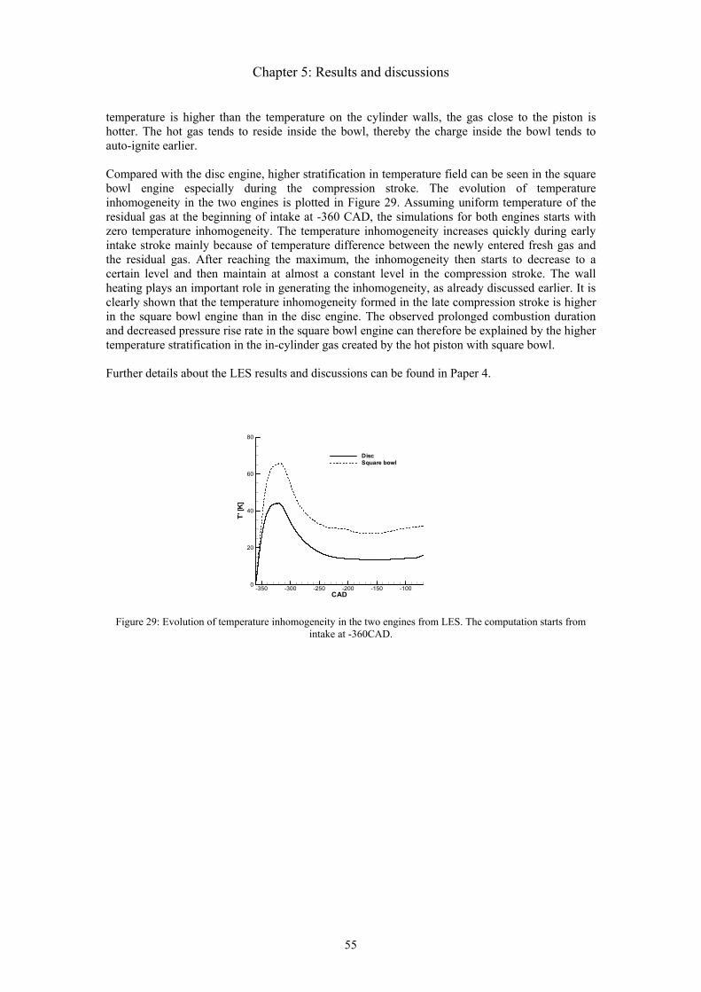
Chapter 5: Results and discussions
55
temperature is higher than the temperature on the cylinder walls, the gas close to the piston is hotter. The hot gas tends to reside inside the bowl, thereby the charge inside the bowl tends to auto-ignite earlier.
Compared with the disc engine, higher stratification in temperature field can be seen in the square bowl engine especially during the compression stroke. The evolution of temperature inhomogeneity in the two engines is plotted in Figure 29. Assuming uniform temperature of the residual gas at the beginning of intake at -360 CAD, the simulations for both engines starts with zero temperature inhomogeneity. The temperature inhomogeneity increases quickly during early intake stroke mainly because of temperature difference between the newly entered fresh gas and the residual gas. After reaching the maximum, the inhomogeneity then starts to decrease to a certain level and then maintain at almost a constant level in the compression stroke. The wall heating plays an important role in generating the inhomogeneity, as already discussed earlier. It is clearly shown that the temperature inhomogeneity formed in the late compression stroke is higher in the square bowl engine than in the disc engine. The observed prolonged combustion duration and decreased pressure rise rate in the square bowl engine can therefore be explained by the higher temperature stratification in the in-cylinder gas created by the hot piston with square bowl.
Further details about the LES results and discussions can be found in Paper 4.
Figure 29: Evolution of temperature inhomogeneity in the two engines from LES. The computation starts from
intake at -360CAD.
CAD
T'[K
]
-350 -300 -250 -200 -150 -1000
20
40
60
80
DiscSquare bowl
Summary of papers
56
6 Summary of papers
Paper 1:
R. Yu, X.S. Bai: A semi-implicit scheme for large eddy simulation of piston engine flows. Manuscript submitted for publication, 2008.
A semi-implicit higher order numerical scheme is developed for large eddy simulation of turbulent reactive flows in piston engines. The numerical scheme is aimed at handling high density ratios in the combustion engines, avoiding wiggles in the physical properties such as species mass fractions, and still maintaining high computational efficiency to meet the highly demanding requirement in simulation of reciprocating engines. The proposed scheme is made up of a fourth order central difference for most of the terms in the transport equations except the convection terms. The latter is discretized using a fifth order WENO scheme to avoid the numerical overshooting of mass fractions. A second order predictor-corrector scheme is used for the time integration. The transport equations are integrated in time using explicit time marching mostly, except for the pressure field and the continuity equation. They are handled using an implicit pressure correction equation of variable coefficient Poisson equation type. This equation is solved numerically using a high efficiency Multi-Grid method that can treat large grid aspect ratio. The numerical scheme is applied to simulate two experimental engines.
Paper 2:
R. Yu, X.S. Bai, H. Lehtiniemi, S.S. Ahmed, F. Mauss, M. Richter, M. Aldén, L. Hildingsson, B. Johansson, A. Hultqvist: Effect of Turbulence and Initial Temperature Inhomogeneity on Homogeneous Charge Compression Ignition Combustion, SAE paper 2006-01-3318, 2006.
A half-liter optical HCCI engine firing a blended fuel (50% n-heptane and 50% iso-octane, air/fuel ratio 3) is studied using LES and laser diagnostics. Formaldehyde and OH LIF and in-cylinder pressure were measured in the experiments to characterize the ignition process. The detailed chemical kinetic mechanism of the blended fuel is provided by S.S. Ahmed. The auto-ignition simulation is coupled with LES by the progress variable method. Systematic LES study on the effect of initial temperature inhomogeneity and turbulence intensity on the ignition process has been carried out. It was shown that the charge under the present experimental condition would not be ignited without initial temperature inhomogeneity. Increasing temperature inhomogeneity leads to earlier ignition whereas increasing turbulence intensity would retard the ignition. This is mostly due to the effect of turbulence on the bulk flow that turbulence tends to decrease the temperature inhomogeneity by enhanced eddy heat transfer. The LES results suggest that desirable ignition timing could be achieved by controlling the turbulence intensity and temperature inhomogeneity.
Paper 3:
R. Yu, X.S. Bai, L. Hildingsson, A. Hultqvist, P. Miles: Numerical and Experimental Investigation of Turbulent Flows in a Diesel Engine, SAE paper 2006-01-3436, 2006.
The turbulence flow field in an optical diesel engine is studied using both LES and Particle Image Velocimetry (PIV). The engine was operated under motored conditions. The PIV velocity measurement near the piston bowl region was compared with LES results. LES is performed continuously throughout one single cycle, starting from intake. The details about structures of the turbulence, the vortex cores, and the temperature field in the entire cylinder were investigated using LES method. The LES uses moving grid consisting of 1283 cells. In the intake phase the large scale swirling and tumbling flow are shown to be responsible the generation of large scale

Summary of papers
57
vortex pipes which break down to small scale turbulent eddies. Different flow structures caused by the shape of piston bowl were shown and explained. The temperature inhomogeneity due to wall heating of nearby gas is also investigated in LES.
Paper 4:
R. Yu, X.S. Bai, A. Vressner, A. Hultqvist, B. Johansson, J. Olofsson, H. Seyfried, J. Sjöholm, M. Richter, M. Aldén: Effect of Turbulence on HCCI Combustion, SAE paper 2007-01-0183, 2007. Accepted for publication in SAE Transactions, Journal of Passenger Cars – Mechanical Systems, 2008.
The combustion process in an optical HCCI engine burning ethanol is studied using LES and experiment. Two different piston shapes, one with a flat disc and the other with a square bowl, were employed to generated different turbulence and temperature field prior to the auto-ignition; the different ignition processes in two engines are compared and explained. It is observed in the experiment the square-bowl engine has longer combustion duration and lower pressure rise rate. The chemiluminescence images show different ignition patterns in two engines: unlike the typical HCCI pattern in the disc engine where ignition kernel appears at multiple positions, the action in the square-bowl engine always starts in the bowl then spreads to the squish region. The experimental observed phenomena are repeated in the spatial and temporal resolved LES. The difference in combustion duration and ignition pattern is explained by LES by the higher temperature inhomogeneity created by the square bowl. LES show the gas temperature in the piston bowl is generally higher than that in the squish, leading to an earlier ignition inside the bowl. Compared with the disc engine, the square-bowl engine has a higher temperature inhomogeneity owing to the turbulent wall heat transfer.
Paper 5:
R. Yu, X.S. Bai: LES of In-cylinder Turbulence and Temperature Stratification in a HCCI Engine, Proc. of ECCOMAS thematic conference on computational combustion, Delft, July 18-20, 2007.
LES with fine grid (2563 cells) is carried out to reveal the well-resolved turbulence structures. Multiple cases have also been simulated with fine grid to study the influence on temperature stratification by several components: the hot residual gas, the wall heating, the piston heating and turbulence mixing. Those components are realized in LES by change temperature of residual gas, wall, piston and using adiabatic walls respectively. The LES cases are designed to study development of temperature stratification both in intake phase and the compression stroke. The turbulent structures are clearly shown by the λ2 vortex, low pressure isocontour and three dimensional stream lines. The temperature stratification is quantified by the temperature Probability Density Function (PDF) which represents the gas temperature distribution in the whole cylinder.
Paper 6:
R. Yu, T. Joelsson, X.S. Bai, B. Johansson: Effect of Temperature Stratification on the Auto-ignition of Lean Ethanol/air Mixture in HCCI Engine, SAE paper 2008-01-1669.
It has been known from multi-zone simulations that HCCI combustion can be significantly affected by temperature stratification of the in-cylinder gas. With the same combustion timing (i.e. crank angles at 50% heat release), large temperature stratification tends to prolong the combustion duration and lower down the in-cylinder pressure-rise-rate. With low pressure-rise-rate HCCI engines can be operated at high load, therefore it is of practical importance to look into more details about how temperature stratification affects the auto-ignition process. It has been realized that multi-zone simulations can not account for the effects of spatial structures of the stratified temperature field, i.e. how the size of the hot and cold spots in the temperature field could affect

Summary of papers
58
the auto-ignition process. This question is investigated in the present work by LES method which is capable of resolving the in-cylinder turbulence field in space and time. The initial temperature field for LES is presumed as the superimposition of a mean temperature and sine-function fluctuating temperature. The engine runs on ethanol with a relative air/fuel ratio of 3.3. The LES results show that the initial shape of hot/cold spots is quickly modified by turbulence. A particular hot/cold spot size on the order of large eddy integral scale is found at which the combustion duration tends to be shorter. This reveals the fact that not only the magnitude of the temperature stratification but also the spatial structure of the stratification could affect the auto-ignition process.
Paper 7:
T. Joelsson, R. Yu, X.S. Bai, A. Vressner, B. Johansson : Large Eddy Simulation and Experiments of the Auto-ignition process of Lean Ethanol/air Mixture in HCCI Engines, SAE paper 2008-01-1668.
Recent experiments and numerical studies have showed that piston geometry has a significant effect on the HCCI process. There are two effects by the combustor geometry: the geometry affects the flow/turbulence in the cylinder; the geometry also affects the temperature stratification. The temperature stratification is more directly responsible for the observed alteration of the auto-ignition process. To investigate this issue further, in this paper we present a study of two engines with the same geometry but difference ways of cooling. Measurement of the two engines – a metal engine and quartz piston engine with the same piston bowl geometry – is carried out and LES is used to simulate the flow, the temperature field and the auto-ignition process. The fuel is ethanol with an air/fuel ratio of 3.3. It is found that lower temperature stratification is established in the metal engine under similar conditions to the optical engine due to the more effective cooling of the piston in the metal engine. The combustion phasing in the two engines are the same by controlling the intake temperature. Both measurements and LES show a more rapid auto-ignition in the metal engine than in the optical engine with the same piston geometry. This confirms the conclusion that having larger temperature stratification could decrease the pressure-rise-rate and thereby increase the load of HCCI engines. The dependence of temperature stratification on the wall temperature and intake temperature is systematically studied using LES.
Note: The candidate has not done any of experimental works in the above papers. All the CFD simulations in the above publications are based on the LES code developed by the candidate.

Conclusion and perspectives
59
7 Conclusion and perspectives
Large eddy simulation of in-cylinder turbulent flows, heat transfer and combustion in HCCI engines is carried out to gain improved understanding of the fundamental physics about the interaction of chemical reactions with heat and mass transport. The approach employed in this work is numerical simulation using spatial and temporal resolved large eddy simulation (LES) models. Major efforts in this work have been put to study the development of turbulence and temperature stratification inside the engine cylinders, and the modeling of the auto-ignition process in HCCI engines. An efficient LES solver has been developed based on a previous in-house code. Several key improvements are made as listed in the following:
• Based on the full implicit scheme in the previous in-house code, a more efficient explicit scheme using fractional-step method is developed;
• A fifth order WENO scheme has been implemented to handle the complex reactive flow systems with high numerical accuracy;
• A predictor-corrector algorithm has been developed to achieve numerical stability in case of high density ratio;
• An improved Multi-Gird (MG) convergence rate under high grid aspect ratio conditions; • An enhanced parallelization procedure based on domain decomposition.
Compared to the RANS approach, LES is able to capture the fine structures in the in-cylinder flow. Several engines with different geometries have been studied using the LES solver. The first engine is a low speed engine with rectangular shape engine chamber which is designed to investigate the tumble flow motion. With this engine configuration the flow field results from LES were validated against the experimental PIV measurements. The second engine is an experimental engine with a practical cylindrical shape combustion chamber. This engine has a flat piston and runs at high speed. For this baseline test engine, high resolution LES with fine grid has been performed and the computational results are investigated in detail. The important flow structures during different stages of engine cycle are examined using three dimensional vortex tubes and streamlines. The large-scale rotational structures caused by the combined tumble and swirl motion appearing in the late compression stage are shown by the iso-surface of globally low hydrodynamic pressure. The influence of piston bowl shape on the in-cylinder turbulent flow is also examined by simulating another two engines with non-flat shape of pistons: a diesel engine with special shape inside the piston bowl and a HCCI engine with square shape inside the piston bowl.
Based on the temperature field predicted by LES, the spatial distribution of possible hot/cold region is analyzed and its correlation with the large scale flow structures is found out. The stratification in temperature field is of particular interest to HCCI combustion. The influence on temperature stratification by several factors, such as residual gas temperature, engine wall temperature, engine piston temperature and adiabatic wall has been studied. Different test cases have been designed to check the effect of these factors separately during the intake stroke and the compression stroke. The temperature stratification is quantified using probability density function of temperature.
With the capacity of more accurately describing the in-cylinder flow and temperature field, the LES method has been extended to simulate the combustion process in HCCI engines. The detailed auto-ignition process is modeled using a reaction progress variable model. The progress variable model is based on numerical tabulation of the auto-ignition process simulated using an independent ignition code with detailed chemical kinetic mechanisms. This approach enables fast and affordable coupling of chemistry with CFD flow simulations. The multi-zone model was used to validate the progress variable model. It is shown that the model can predict the effect of temperature stratification on HCCI combustion process rather satisfactorily.

Conclusion and perspectives
60
With the progress variable model, LES has been applied to study the auto-ignition process in laboratory HCCI engines. In several HCCI experiments, the ignition patterns and combustion characteristics (such as the pressure-rise-rate and the combustion duration) are found to be significantly influenced by different piston bowl shapes (i.e. square bowl piston vs. flat piston) and also different piston materials and cooling (metal vs. quartz). The experimentally observed phenomena are well repeated in LES. Based on the LES results, an explanation of these physical and chemical processes is obtained. It is concluded that the level of temperature stratification formed in the cylinder is rather sensitive to the piston geometry and cooling of the walls, and this is more directly responsible for the experimentally observed combustion phenomena. Systematic studies have been carried out using LES to investigate how HCCI combustion can be affected by in-cylinder turbulence, and the length scales of the temperature stratification.
Further works are desirable for the future:
• First, there is a need to develop more accurate models for coupling of the chemical kinetic mechanisms to CFD flow simulations. The current reaction progress variable model needs to be extended and validated for different fuels and for conditions with direct injection of fuel to the cylinders and with high level of exhaust gas recirculation to the cylinder.
• LES has the potential to simulate fairly accurately the temperature stratification in the cylinder. The accuracy of this type of simulation is not yet well explored due to the lack and difficult of detailed experimental data in the engine cylinders. A combined experimental and LES study of the in-cylinder temperature field is desirable.

References
61
8 References
1. N. Iida, T. Ichikura, K. Kase, Y. Enomoto: Self-ignition and combustion stability in methanol fueled low heat rejection ceremic ATAC engine – analysis of cyclic varaiation at high wall temperatures and lean burn operation. JSAE paper 9733684, 1997.
2. F. Zhao: Homogeneous charge compression ignition (HCCI) engines: key research and development issues. SAE International, USA, 2003.
3. N. Peters, F.A. Williams: The asymptotic structure of stoichiometric methane/air flames. Combustion and Flame 68, 185-207, 1987.
4. J. Buckmaster, P. Clavin, A. Linan, M. Matalon, N. Peters, G. Sivashinsky, F.A. Williams: Combustion theory and modeling, Proc. Combust. Inst. 30, 1-20, 2005.
5. J. Nygren, J. Hult, M. Richter, M. Alden, M. Christensen, A. Hultqvist, B. Johansson: Three-dimensional laser induced fluorescence of fuel distributions in an HCCI engine. Proceedings of the Combustion Institute 29, 679-685, 2002.
6. S.O.H. Jo, K. Shoda, P.D. Jo, S. Kato: Active thermo-atmosphere combustion (ATAC). SAE paper 790501, 1979.
7. J.R. Smith, S.M. Aceves, C.K. Westbrook, W. Pitz: Modeling of homogeneous charge compression ignition of methane. ASME International 1997 Fall Conference, Madison, Wisconsin, USA, 1997.
8. M. Christensen, B. Johansson, P. Einewall: Homogeneous charge compression ignition (HCCI) using iso-octane, ethanol and natural gas – a comparison with spark ignition operation. SAE paper 972874, 1997.
9. M. Christensen, B. Johansson, P. Amneus, F. Mauss: Supercharged homogeneous compression ignition. SAE paper 980787, 1998.
10. M. Richter, A. Franke, M.A. A., A. Hultqvist, B. Johansson: Optical diagnostics applied to naturally aspirated homogeneous charge compression ignition engine. SAE paper 1999-01-3649, 1999.
11. M. Richter, A. Franke, J. Engstrom, A. Hultqvist, B. Johansson, M. Alden: The influence of charge inhomogeneity on the HCCI combustion process. SAE paper 2000-01-2868, 2000.
12. R. Collin, J. Nygren, M. Richter, M. Alden, L. Hindingsson, B. Johansson: Simultaneous OH and formaldehyde measurements in a HCCI engine. SAE paper 2003-01-3218, 2003.
13. M. Kraft, P. Maigaard, F. Mauss, M. Christensen, B. Johansson: Investigation of combustion emission in a homogeneous charge compression injection engine:measurements and a new computational model. Proc. Combust. Inst. 28, 1195-1201, 2000.
14. D.L. Flowers, S.M. Aceves, J. Martinez-Frias, R.W. Dibble: Prediction of carbon monoxide and hydrocarbon emissions in iso-octane HCCI engine combustion using multizone simulation. Proc. Comust. Inst. 29, 687-694, 2002.
15. Y.B. Zeldovich: Regime classification of an exhothermic reaction with nonuniform initial condition. Combustion and Flame 39, 211-214, 1980.
16. R. Sankaran, H.G. Im: Characteristics of auto-ignition in a stratified iso-octane mixture with exhausti gases under homogeneous charge compression ignition conditions. Combustion Theroy and Modeling 9, 417-432, 2005.
17. A. Hultqvist, M. Christensen, B. Johansson, M. Richter, J. Nygren, J. Hult, M. Alden: The HCCI combustion process in a single cycle high-speed fuel tracer LIF and chemiluminescence imaging. SAE paper 2002-01-0424, 2002.
18. P. Nilsson, X.S. Bai: Effect of Flame Stretch and Wrinkling on CO Formations in Turbulent Premixed Flames. Proc. Combust. Inst. 29, 1873-1879, 2002.
19. P. Wang, X.S. Bai: Large eddy simulation of turbulent premixed flames using level-set G-equation. Proc. Combust. Inst. 30, 583-591, 2005.
20. P. Amneus, D. Nilsson, F. Mauss, M. Christensen, B. Johansson: Homogeneous charge compression ignition engine: experiments and detailed kinetic calculations. COMODIA'98 9, 567-572, 1998.
21. P.L. Kelly-Zion, J.E. Dec: A computational study of the effect of fuel type on ignition time in homogeneous charge compression ignition engines. Proc. Combust. Inst. 28, 1187-1194, 2000.
22. S.M. Aceves, D.L. Flowers, C.K. Westbrook, J.R. Smith, W. Pitz, R.W. Dibble, M. Christensen, B. Johansson: A multizone model for prediction of HCCI combustion and

References
62
emissions. SAE paper 2000-01-0327, 2000. 23. S.M. Aceves, D.L. Flowers, J. Martinez-Frias, J.R. Smith, C.K. Westbrook, W.J. Pitz, R.W.
Dibble, J.F. Wright, W.C. Akinyemi, R.P. Hessel: A sequential fluid mechanics chemical kinetics model of propane HCCI combustion. SAE paper 2001-01-1027, 2001.
24. S.C. Kong, R.D. Reitz: Application of detailed chemistry and CFD for predicting direct injection HCCI engine combustion and emissions. Proc. Combust. Inst. 29, 663-669, 2002.
25. S.C. Kong, R.D. Reitz: Numerical simulation of premixed HCCI engine combustion and its sensitivity to computational mesh and model uncertainties. Combust. Theory Modelling 7, 417-434, 2003.
26. S.A. Slimon, M.C. Soteriou, D.W. Davis: Development of computational aeroacustics equations for subsonic flows using a Mach number expansion approach. Journal of Computational Physics 159, 377-466, 2000.
27. S.S. Ahmed, G. Moréac, T. Zeuch, F. Mauss: Reduced mechanism for the oxidation of the mixtures of n-heptane and iso-octane. Proceedings of the European Combustion Meeting, Louvain-la-Neuve, Belgium, 2005.
28. S.M. Aceves, D.L. Flowers, J. Martinez-Frias, F. Espinosa-Loza, M. Christensen, B. Johansson, R.P. Hessel: Analysis of the effect of geometry generated turbulence on HCCI combustion by multi-zone modeling. SAE 2005-01-2134, 2005.
29. H. Lehtiniemi, F. Mauss, M. Balthasar, I. Magnusson: Modeling diesel engine combustion with detailed chemistry using a progress variable approach. SAE paper 2005-01-3855, 2005.
30. O. Colin, A. Pires, d. Cruz, S. Jay: Detailed chemistry based auto-ignition model including low temperature phenomena applied to 3D engine calculations. Proc. Combust. Inst. 30, 2649-2656, 2005.
31. Y. Zhang, B. Rogg, K.N.C. Bray: 2-D Simulation of Turbulent Autoignition with Transient Laminar Flamelet Source Term Closure. Combust. Sci. and Techn. 105, 211-227, 1995.
32. S.S. Ahmed: Licentiate thesis. Lund Institute of technology, 2004. 33. N.M. Marinov: A Detailed Chemical Kinetic Model for High Temperature Ethanol Oxidation.
Int. J. Chem. Kinet 31, 183-220, 1999. 34. R.J. Kee, J.A. Miller, T.H. Jefferson: CHEMKIN. A General Purpose, Problem-Independent,
Transportable, FORTRAN Chemical Kinetics Code. Technical Report SAND 8003, Sandia National Laboratories, 1980.
35. Cantera, An open source code for problems involving chemically-reacting flows, http://www.cantera.org/.
36. P.C. Miles: Turbulent flow structure in direct-injection, swirl-supported diesel engines – A chapter in “Flow and Combustion in Reciprocating Engines”, Edited by C. Arcoumanis and T.Kamimoto, Experimental Fluid Mechanics 2008.
37. S. Richarda, O.C.O. Vermorela, A. Benkenidaa, C. Angelbergera, D. Veynanteb: Towards large eddy simulation of combustion in spark ignition engines. Proceedings of the Combustion Institute 31, 3059-3066, 2007.
38. D.C. HAWORTH: Large-Eddy Simulation of In-Cylinder Flows. Oil & Gas Science and Technology - Rev. IFP 54, 175 - 185, 1999.
39. U. Piomelli, E. Balaras: Wall-Layermodels For Large-Eddy Simulations. Annu. Rev. Fluid Mech 34, 349–374, 2002.
40. P. Wang, X.S. Bai, M. Wessman, J. Klingman: Experimental and LES of Swirling Turbulent Flows in a Model Gas Turbine Combustor. Physics of Fluids 16, 3306-3324, 2004.
41. T. Poinsot: Large Eddy simulation of combustion instabilities in gas turbines. IUTAM workshop on DNS and LES. Kingston, Canada, 2001.
42. P. Schmitt, B. Schuermans, K.P. Geigle, T. Poinsot: Effects of radiation, wall heat loss and effusion cooling on flame stabilisation and pollutant prediction in LES of gas turbine combustion. ECCOMAS thematic conference on computational combustion, Lisbon, 21-24 Juin., 2005.
43. G. Boudier, L. Gicquel, T. Poinsot, D. Bissières, C. Berat: Comparison of LES, RANS and Experiments in an Aeronautical Gas Turbine Combustion Chamber. Proc. Comb. Institute 31, 2006.
44. P. Schmitt, T. Poinsot, B. Schuermans, P. Geigle: Large-eddy simulation and experimental study of heat transfer, nitric oxide emissions and combustion instability in a swirled turbulent high-pressure burner. J. Fluid Mech 570, 17–46, 2007.
45. F.d. Mare, W. P.Jones, K.R. Menzies: Large eddy simulation of a model gas turbine combustor.

References
63
Combust. Flame 137, 278-294, 2004. 46. C. Meneveau, J. Katz: Scale-Invariance and Turbulence Models for Large-Eddy Simulation.
Annual Review of Fluid Mechanics 32, 1-32, 2000. 47. J. Smagorinsky: General Circulation Experiments with the Primitive Equations. I. The Basic
Experiment. Monthly Weather Review 91, 99-164, 1963. 48. D.K. Lilly: On the Application of the Eddy Viscosity Concept in the Inertial Subrange of
Turbulence. NCAR Manuscript 123, 1966. 49. S. B.Pope: Turbulent flows, Cambridge university press 2000. 50. J.Gullbrand, X.S. Bai, L.Fuchs: High-order Cartesian grid method for calculation of
incompressible turbulent flows. International journal for numerical methods in fluids 36, 687-709, 2000.
51. X.S. Bai: On the modeling of turbulent combustion at Low Mach numbers. Royal Institute of Technology, Stockholm, Doctoral thesis, 1994.
52. C.W. Shu, S. Osher: Efficient implementation of essentially non-oscillatory shock-capturing schemes. Journal of Computational Physics 77, 439-471, 1988.
53. G.S. Jiang, C.W. Shu: Efficient Implementation of Weighted ENO Schemes. Journal of Computational Physics 126, 202, 1996.
54. A. Harten, B. Engquist, S. Osher, S. CHAKRAVARTHY: Uniformly high order accurate essentially non-oscillatory schemes, III. Journal of Computational Physics 131, 3-47, 1997.
55. M. Salewski: LES of Jets and Sprays injected into crossflow. Lund university, Doctoral thesis, 2006.
56. J. Kim, P. Moin: Application of a fractional-step method to incompressible Navier-Stokes equations. Journal of Computational Physics 59, 308-323, 1985.
57. J.H. Ferziger, M. Peric: Computational Methods for Fluid Dynamics, Springer-Verlag, 1997. 58. A.W. Cook, J.J. Riley: Direct Numerical Simulation of a Turbulent Reactive Plume on a
Parallel Computer. Journal of Computational Physics 129, 263-283, 1996. 59. C.D. Pierce: Progress-Variable Approach for Large-Eddy Simulation of Turbulent combustion.
Stanford, 2001. 60. F. Nicoud: Conservative High-Order Finite-Difference Schemes for Low-Mach Number Flows
Journal of Computational Physics 158, 71-97, 2000. 61. A.S. Almgren, J.B. Bell, P. Colella, L.H. Howell, M.L. Welcome: A conservative adaptive
projection method for the variable density incompressible Navier-Stokes equations. Journal of Computational Physics 142, 1-46, 1998.
62. J.B. Bell, M.S. Day, C.A. Rendleman, S.E. Woosley, M.A. Zingale: Adaptive low Mach number simulations of nuclear flame microphysics. Journal of Computational Physics 195, 677-694, 2004.
63. M.S. Day, J.B. Bell: Numerical simulation of laminar reacting flows with complex chemistry. Combustion Theory Modeling 4, 535-556, 2000.
64. P. Wang: Large Eddy Simulation of Turbulent Swirling Flows and Turbulent Premixed combustion. Lund University, doctoral thesis, 2005.
65. O.M. Knio, H.N. Najm, P.S. Wyckoff: A semi-implicit Numerical Scheme for Reacting Flow, II. Stiff Operator-Split Formulation. Journal of Computational Physics 154, 428-467, 1999.
66. H.N. Najm, P.S. Wyckoff, O.M. Knio: A semi-implicit Numerical Scheme for Reacting Flow, I. Stiff Chemistry. Journal of Computational Physics 141, 381-402, 1998.
67. B.L. Miltiadis, V. Papalexandris: Time-accurate calculation of variable density flows with strong temperature gradients and combustion. Journal of Computational Physics 212, 218-246, 2006.
68. G. Pöplau, U.v. Rienen, B.v.d. Geer, M.d. Loos: Multigrid Algorithms for the Fast Calculation of Space-Charge Effects in Accelerator Design. IEEE TRANSACTIONS ON MAGNETICS 40(2), 2004.
69. G. Poplau, U.V. Rienen: Multigrid Solvers for Poisson’s Equation in Computational Electromagnetics. Scientific Computing in Electrical Engineering, LNCSE 18, Springer–Verlag, Berlin, 169 - 176, 2001.
70. J. Larsson, F.S. Lien, E. Yee: Conditional semicoarsening multigrid algorithm for the Poisson equation on anisotropic grids. Journal of Computational Physics 208, 368–383, 2005.
71. OpenFOAM: The Open Source Computational Fluid Dynamics (CFD) Toolbox, http://www.opencfd.co.uk/openfoam/.
72. J. Boree, S. Maurel, R. Bazile: Disruption of a compressed vortex. Physics of fluids 14,

References
64
2543-2556, 2002. 73. S.Maurel, J.Boree, R.Bazile: Experimental Database on a compressed vortex, Private
communication. 74. M.S. Toledo, L.L. Penven, M. Buffata, A. Cadiou, J. Padillaa: Large eddy simulation of the
generation and breakdown of a tumbling flow. International Journal of Heat and Fluid Flow 28, 113-126, 2007.
75. R.H. Kraichnan: Diffusion by a Random Velocity Field. The physics of fluids 13, 22-31, 1970. 76. A.Careta, F. Sagues: Stochastic generation of homogenous isotropic turbulence with
well-defined spectra. Physical Review E 48(3), 1993 77. J.B. Heywood: Internal combustion engine fundamentals, McGRAW-HILL 1988. 78. T. Tennekes, J.L. Lumley: A first course in turbulence, MIT Press 1972. 79. H.J. Lugt: The dilemma of defining a vortex. in Recent Developments in Theoretical and
Experimental Fluid Mechanics. ed. K.G.R. U. Müller, B. Schmidt, Springer, 1979. 80. J. Jeong, F. Hussain: On the identification of a vortex. Journal of Fluid Mechanics 285, 69-94,
1995. 81. A. Vressner: Studies on the load range of an HCCI engine using in-cylinder pressure, ion
current and optical diagnostics, Ph.D. thesis, in Division of Combustion Engines. Lund Institute of Technology, Lund, 2007.
82. A. Hultqvist: Characterization of the homogeneous charge compression ignition processm, Ph.D thesis, in Division of Combustion Engines. Lund Institute of Technology, Lund, 2002.
83. H. Ryo: Laser diagnostics for combustion chemical species and temperature in premixed charge combustion engines, Licentiate thesis Lund Institute of Technology, 2006.
84. A. Vressner, A. Hultqvist, B. Johansson: Study on Combustion Chamber Geometry Effects in an HCCI Engine using High-Speed Cycle-Resolved Chemiluminescence Imaging. SAE 2007-01-0217, 2007.
85. H. Seyfried, J. Olofsson, J. Sjöholm, M. Richter, M. Aldén, A. Vressner, B. Hultqvist, B. Johansson: High-Speed PLIF Imaging for Investigation of Turbulence on Heat Release Rates in HCCI Combustion. SAE 2007-01-0213, 2007.


![Large Eddy Simulation of Supersonic Combustion …...requireaveryfinemesh,unlikequasi-linearapproaches[3],andarethereforepromisingfor turbulence-combustion modelling. The first compressible](https://static.fdocuments.us/doc/165x107/5ed501b48272e64a824742e6/large-eddy-simulation-of-supersonic-combustion-requireaveryfinemeshunlikequasi-linearapproaches3andarethereforepromisingfor.jpg)