Large-Eddy Simulation of Evaporating Spray

in a Coaxial Combustor

Sourabh V. ApteSchool of Mechanical, Industrial and Manufacturing Engineering, Oregon State

University, Corvallis, OR 97331

Krishnan MaheshDepartment of Aerospace Engineering and Mechanics, University of Minnesota,

Minneapolis, MN 55455

Parviz MoinCenter for Turbulence Research, Stanford University, Stanford, CA 94305

Corresponding Author

Sourabh V. Apte, Oregon State University, 204 Rogers Hall, Corvallis, OR 97331,

USA,

email: sva@engr.orst.edu, phone: 541-737-7335, fax: 541-737-2600

Colloquium: SPRAY and DROPLET COMBUSTION

32nd International Symposium on Combustion

Word Count (Method M1, manual count)

Abstract: 278 words

Total Main Body Text: 6139 words

Text: 4255 words (340 lines of text), Equations: 320 words (15 equations), Figures

and Caption: 1000 words (6 figures), References: 524 words (28 references),

Acknowledgements: 40 words

Preprint submitted to Elsevier 11 June 2008

Abstract

Large-eddy simulation of an evaporating isopropyl alcohol spray in a coaxial combus-

tor is performed. The Favre-averaged, variable density, low-Mach number Navier-

Stokes equations are solved on unstructured grids with dynamic subgrid scale model

to compute the turbulent gas-phase. The original incompressible flow algorithm

for LES on unstructured grids by Mahesh et al. (J. Comp. Phy., 2004, 197, 215–

240) is extended to include density variations and droplet evaporation. An efficient

particle-tracking scheme on unstructured meshes is developed to compute the dis-

persed phase. Experimentally measured droplet size distribution and size-velocity

correlation near the nozzle exit are used as the inlet conditions for the spray. The

predictive capability of the LES approach on unstructured grids together with La-

grangian droplet dynamics models to capture the droplet dispersion characteristics,

size distributions, and the spray evolution is examined in detail. The mean and tur-

bulent quantities for the gas and particle phases are compared to experimental data

to show good agreement. It is shown that for low evaporation rates considered in the

present study, a well resolved large-eddy simulation together with simple subgrid

models for droplet evaporation and motion provides good agreement of the mean

and turbulent quantities for the gas and droplet phases compared to the experi-

mental data. This work represents an important first step to assess the predictive

capability of the unstructured grid LES approach applied to spray vaporization.

The novelty of the results presented is that they establish a baseline fidelity in the

ability to simulate complex flows on unstructured grids at conditions representative

of gas-turbine combustors.

Key words: Sprays, LES, unstructured grids, particle-laden flows,

Eulerian-Lagrangian

2

1 Introduction

Turbulent multi-phase flows are encountered in a variety of engineering applications; e.g. internal

combustion engines, liquid and solid propellant rocket motors, gas-turbine aircraft engines, cy-

clone combustors, and biomass gasifiers. The physics of such flows is extremely complex. In gas

turbine combustors, for example, the liquid fuel jet undergoes primary and secondary atomiza-

tion, the resulting droplets evaporate/condense and collide/coalesce, fuel and oxidizer then mix

yielding spray-flames. In addition, realistic combustor configurations make accurate numerical

predictions a challenging task. High-fidelity simulations of these flows require use of accurate nu-

merical schemes with good conservative properties and advanced sub-grid models to capture the

physical phenomena associated with both phases. To build a comprehensive numerical approach

with good predictive capability for such flows, a systematic development and validation of new

schemes and models are necessary. It is also important to investigate limitations of any simplify-

ing assumptions, and their potential impact on the flow evolution. In the present work, emphasis

is placed on simulation and analysis of evaporating spray in a coaxial combustion chamber where

detailed experimental data together with well-specified boundary conditions are available. The

approach is based on large-eddy simulation on unstructured grids [1] with the potential of sim-

ulating complex flows in realistic configurations. The predictive capability of this approach with

subgrid scale models for spray evaporation is evaluated.

Most numerical investigations of particle-turbulence interactions with large number of particles

(on the order of millions) use DNS [2–4], LES [5,6] or RANS [7] for the continuum carrier phase

and a ‘point-particle (PP)’ assumption for the dispersed phase. The dispersed phase is assumed

subgrid so that the particle size (dp) is assumed smaller than the Kolmogorov length scale (LK)

for DNS, and dp is smaller than the grid size (∆) in LES or RANS. However, in LES (or RANS),

3

only the spatially filtered, φ = φf − φsgs (or time-averaged, 〈φ〉 = φf − φ′), flow quantities (fluid

velocities, species mass fractions, and temperature) are computed. Effect of the subgrid-scale

quantities, φsgs (or φ′ in RANS) should be modeled to correctly represent the forces on the

particle.

Considerable effort has been devoted to reconstruct the effect of unresolved velocity fluctuations

(usgs) on the particle motion using statistical methods, stochastic theory and Langevin mod-

els [8,9]. It has been shown that one-point statistics such as particle dispersion, velocity fluctua-

tions, and time-scales are less sensitive to the subgrid-scale velocity fluctuations. For evaporating

droplets, a priori studies on subgrid scale modeling have also been performed [10]. Reveillon &

Vervisch [11] showed that for evaporating sprays, droplet vaporization adds additional unclosed

terms in the evaluation of the mixture fraction variance field. Both the scalar dissipation rate

and the mixing characteristics are affected, as a result.

Recently, simulations of solid particle-laden turbulent flow by Apte et al. [6], neglected the direct

effect of the subgrid velocity fluctuations on particle motion and showed excellent agreement

with experimental data. It was found that if the energy content in the subgrid scale is small

compared to the resolved scale kinetic energy, the influence of the subgrid velocity is typically

negligible. This approach was further extended to model liquid fuel atomization using a stochastic

model for secondary breakup and showed good agreement with experimental data [12]. However,

evaporating-droplet laden flow was not simulated.

Menon and co-workers [13] have performed large-eddy simulations of non-reacting and reacting

flows in a swirling combustion chamber with liquid spray in complex configuration. They showed

good predictive capability of LES in capturing spray evolution, droplet dispersion, and turbulence

modulation by droplets in the presence of heat release. There approach is based on compressible

Navier-Stokes equations in generalized coordinates. In order to represent complex passages in

4

combustors with relatively easy grid generation, use of unstructured grids is necessary. Mahesh

etal. [1,14] developed new algorithms for LES of single-phase non-reacting and reacting flows

in complex configurations and showed the effectiveness of LES in combustor geometries. In the

present work, we extend their formulation for incompressible flows to variable-density flows at

low-Mach numbers (as those encountered in gas-turbine combustors) to include physics of droplet

vaporization, droplet dispersion, and turbulent mixing of fuel vapor and oxidizer. Emphasis is

placed on the predictive capability of a well-resolved LES on unstructured grids to capture the

mean and standard deviations in droplet size and velocity distributions.

Sommerfeld et al. [15] provide detailed measurements of an evaporating isopropyl alcohol spray in

a model combustion chamber. Detailed measurements of the droplet size distributions very near

the injector were performed in addition to one-component phase-Doppler-anemometer (PDA)

measurements to obtain mean and rms gas-phase and droplet-phase statistics of velocity and

particle size. Since detailed droplet size distributions and size-velocity correlations near the in-

jector nozzle are available, these can be used as inflow conditions for the liquid spray, thus elim-

inating any uncertainties associated with spray atomization and secondary breakup modeling.

RANS-based modeling of this experimental setup with Eulerian-Lagrangian approach [16] and

joint-pdf based Eulerian-Eulerian approach [17] have been reported. The RANS simulations [16]

indicated strong sensitivity of predicted results to the number of computational parcels used in

the simulation. LES study of this test case on unstructured grids has not been conducted and rep-

resents an important step to assess the predictive capability of flow solvers specifically developed

for complex combustor configurations. Detailed measurements as reported by this experimental

study are typically not feasible in realistic geometries and thus this data provides an excellent

benchmark case for validating evaporating spray models.

5

2 Mathematical Formulation

The mathematical formulation is based on the variable density, low-Mach number equations for

the fluid phase. Any acoustic interactions and compressibility effects are neglected. In addition,

in writing the energy equation, we invoke the low-Mach number assumptions together with unity

Lewis number. Also the viscous dissipation and Dufour effects are assumed negligible.

2.1 Gas-Phase Equations

The Favre-averaged governing equations for LES of the low-Mach number, variable density flow

are given below,

∂ρg∂t

+∂ρguj∂xj

= Sm, (1)

∂ρgui∂t

+∂ρguiuj∂xj

= − ∂p

∂xi+

∂

∂xj

(2µSij

)− ∂qij∂xj

+ Si, (2)

∂ρgZ

∂t+∂ρgZuj∂xj

=∂

∂xj

(ρgαZ

∂Z

∂xj

)− ∂qZj

∂xj+ SZ , (3)

∂ρgh

∂t+∂ρghuj∂xj

=∂

∂xj

(ρgαh

∂h

∂xj

)− ∂qhj∂xj

+ Sh, (4)

where Sij = 12

(∂ui

∂uj+ ∂uj

∂ui

)− 1

3δij

∂uk

∂xk, and ρg is the density of the gaseous mixture, Z is the filtered

mixture fraction, ui is the velocity, µ is the viscosity, p is the pressure, h =∑i Yihi(T ) is the

total mixture enthalpy, S are the source terms due to inter-phase coupling. The subgrid scale

unclosed transport terms in the momentum, scalar, and enthalpy equations are grouped into the

residual stress qij, and residual scalar flux qZj, qhj. The dynamic Smagorinsky model by Moin et

al. [18,19] is used. The dynamic model has no adjustable constants, and thus allows evaluation

of the predictive capability of the model.

6

For the present study, no chemical reactions are considered and chemical source terms are absent.

The liquid droplets evaporate and the resulting fuel vapor undergoes pure mixing with the

surrounding air. Unlike a two-inlet pure gaseous system, the fuel in the above formulation is in

the liquid form. This implies that the maximum value of vapor fuel mass fraction is dependent

on the local saturation conditions around a drop.

The source terms in the gas-phase continuity, mixture-fraction, and momentum equations are

obtained from the equations governing droplet dynamics (Eqs. 8, 9). For each droplet the

source terms are interpolated from the particle position (xp) to the centroid of the grid control

volume using an interpolation operator. The source terms in the continuity and mixture fraction

equations are identical as they represent conservation of mass of fuel vapor. The expressions for

source terms are:

Sm(x) = SZ(x) = −∑k

Gσ(x,xp)d

dt(mp) (5)

Si(x) = −∑k

Gσ(x,xp)d

dt

(mpu

kpi

)(6)

Sh(x) = −∑k

Gσ(x,xp)d

dt(mpCp,`Tp) (7)

where the summation is over all droplets (k). The function Gσ is a conservative interpolation

operator with the constraint∫VcvGσ(x,xp)dV = 1 [6], and Vcv is the volume of the grid cell in

which the droplet lies.

2.2 Liquid-Phase Equations

Droplet dynamics are simulated using a Lagrangian point-particle model. It is assumed that (1)

the density of the droplets is much greater than that of the carrier fluid, (2) the droplets are

7

dispersed and collisions between between them are negligible, (3) the droplets are much smaller

than the LES filter width, (4) droplet deformation effects are small, and (5) motion due to shear

is negligible. Under these assumptions, the Lagrangian equations governing the droplet motions

become [20]

dxpdt

= up;dupdt

=1

τp(ug,p − up) +

(1− ρg

ρp

)g (8)

where xp is the position of the droplet centroid, up denotes the droplet velocity, ug,p the gas-

phase velocities interpolated to the droplet location, ρp and ρg are the droplet and gas-phase

densities, and g is the gravitational acceleration. The droplet relaxation time scale (τp) is given as:

τp = ρpd2p/[18µg(1 + aRebp)], where dp is the diameter and Rep = ρgdp|ug,p−up|/µg is the droplet

Reynolds number [20]. The above correlation is valid for Rep ≤ 800. The constants a = 0.15, b =

0.687 yield the drag within 5% from the standard drag curve. It should be noted that these

assumptions are valid in regions of dilute spray where the droplet size is smaller than the LES filter

width. Near the injector the droplets are densely packed, and undergo collision and coalescence.

In addition, the grid resolution may become comparable to droplet size. Under these assumptions,

the point-particle approach is not valid. Recently, Apte et al. [21] investigated a mixture-theory

based model taking into account the volumetric displacements in dense particulate flows to show

significant influences on the flow field. In the present simulation, the spray breakup process is not

simulated, the droplet size distribution measured in the experiments is used as an inlet condition,

and further away from the injection point, the spray becomes dilute. However, a model taking

into account the volumetric fluid displacement caused by droplet motion should be considered

in regions of dense spray.

The droplet evaporation is modeled based on an equilibrium ‘uniform-state’ model for an isolated

droplet [22–24]. Miller et al [25] investigated different models for evaporation accounting for non-

8

equilibrium effects. In the present work, non-equilibrium effects are neglected since the rates of

evaporation are slow for the low gaseous temperatures used in the experiment. Advanced models

considering internal circulation, temperature variations inside the droplet, effects of neighboring

droplets [24] may alter the heating rate (Nusselt number) and the vaporization rates (Sherwood

number). However, for the present case of non-reacting flow, the evaporation is dominated by

mass-diffusion, the rates are low, and hence these effects are neglected. The Lagrangian equations

governing droplet temperature and mass become [22–24]

dmp

dt= −mp

τm;

dTpdt

=1

τc

(Tg,p − T sp

)− 1

τm

∆hvCp,`

(9)

where ∆hv is the latent heat of vaporization, mp mass of the droplet, Tp temperature of the

droplet, T sp is the temperature at the droplet surface, Tg,p is the temperature of the gas-phase at

the droplet location and Cp,` is the specific heat of liquid. The diameter of the droplet is obtained

from its mass, dp = (6mp/πρp)1/3. Here, τm and τc are the droplet life-time and the convective

heating time-scales respectively, and are given as

1

τm=

12

d2p

Dsln(1 +BY )Sh;1

τc=

12

ρpd2p

ks

Cp,`

ln(1 +BT )

BT

Nu. (10)

Here, D and k are the diffusivity and conductivity, respectively. The superscript s stands for

droplet surface and Sh and Nu are the Sherwood and Nusselt numbers given as

Sh = 1 +0.278Re1/2

p [Scs]1/3√1 + 1.232/Rep[Scs]1/3

; Nu = 1 +0.278Re1/2

p [Prs]1/3√1 + 1.232/Rep[Prs]1/3

. (11)

BY and BT are the mass diffusion and heat transfer coefficients, respectively. For T sp < Tb (where

Tb is the boiling point), BY = (Y sF − YF g,p)/(1− Y s

F ) and BT = Csp(Tg,p − T sp )/(∆hv), where YF g,p

is the fuel vapor mass-fraction interpolated to the droplet location. For T sp ≥ Tb, BY is set equal

to BT . The Clausius-Clapeyron equilibrium vapor-pressure relationship is used to compute the

9

fuel mass-fraction at the droplet surface. Liquid properties are evaluated using the 1/3rd rule for

reference mass fractions [22].

2.3 Subgrid Scale Modeling

In LES of droplet-laden flows, the droplets are presumed to be subgrid, and the droplet-size is

smaller than the filter-width used. The gas-phase velocity field required in Eq. (8) is the total

(unfiltered) velocity, however, only the filtered velocity field is computed in Eqs. (2). The direct

effect of unresolved velocity fluctuations on droplet trajectories depends on the droplet relaxation

time-scale, and the subgrid kinetic energy. Pozorski & Apte [8] performed a systematic study

of the direct effect of subgrid scale velocity on particle motion for forced isotropic turbulence.

It was shown that, in poorly resolved regions, where the subgrid kinetic energy is more than

30%, the effect on droplet motion is more pronounced. A stochastic model reconstructing the

subgrid-scale velocity in a statistical sense was developed [8]. However, in well resolved regions,

where the amount of energy in the subgrid scales is small, this direct effect was not strong. In

the present work, the direct effect of subgrid scale velocity on the droplet motion is neglected.

However, note that the particles do feel the subgrid scales through the subgrid model that affects

the resolved velocity field. For well-resolved LES of swirling, separated flows with the subgrid

scale energy content much smaller than the resolved scales, the direct effect was shown to be

small [6].

In addition, work by Masoudi and Sirignano [26] has shown that collisions between subgrid scale

vortices and droplet sizes can modify the Nusselt and Sherwood numbers used in convective cor-

rection factors (Eq. 10). In the present case the evaporation rates are low and are not significantly

affected by these effects. However, in general these effects need to be investigated in the context

10

of LES.

To account for the effects of the SGS turbulence, the filtered mass fractions and temperature

fields are correlated with the mixture fraction, Yi = Yi(Z, Z ′′2). In the present work, a presumed

beta-pdf approach is used to evaluate the filtered mass-fraction fields:

Yi =∫Yi(ζ)PZ(ζ)dζ; PZ(ζ) =

ζa−1(1− ζ)b−1∫ 10 ζ

+a−1(1− ζ+)b−1dζ+; (12)

where a = ZZs

((Z/Zs)(1−Z/Zs)

Z′′2/(Zs)2 − 1

)and b = a

(1

Z/Zs − 1). Here, Zs is the local saturation mixture

fraction and is obtained by averaging the surface values of fuel mass fractions over all droplets

in a given control volume. The beta pdf used here ensures that PZ is properly defined in the

range 0 ≤ Z ≤ Zs [11]. The mixture fraction variance Z ′′2 is modeled as ρZ ′′2 = CZρ∆2|∇Z|2,

where ∆ is the filter width, and the coefficient CZ is obtained using the dynamic procedure [19].

This implicitly assumes that the time-scale of evaporation is small compared to the scalar mixing

time-scale. However, use of more advanced micro-mixing models [11] may become necessary in

the presence of chemical reactions.

3 Numerical Method

The computational approach is based on a co-located, finite-volume, energy-conserving numerical

scheme on unstructured grids [14] and solves the low-Mach number, variable density gas-phase

flow equations. Numerical solution of the governing equations of continuum phase and particle

phase are staggered in time to maintain time-centered, second-order advection of the fluid equa-

tions. Denoting the time level by a superscript index, the velocities are located at time level tn

and tn+1, and pressure, density, viscosity, and the scalar fields at time levels tn+3/2 and tn+1/2.

Droplet position, velocity and temperature fields are advanced explicitly from tn+1/2 to tn+3/2

11

using fluid quantities at time-centered position of tn+1. In this co-located scheme, the velocity

and pressure fields are stored and solved at the centroids of the control volumes.

Lagrangian droplet equations:

The droplet equations are advanced using a third-order Runge-Kutta scheme. Owing to the

disparities in the flowfield time-scale (τf ), the droplet relaxation time (τp), the droplet evaporation

time-scale (τm), and the droplet heating time-scale (τc), sub-cycling of the droplet equations

becomes necessary. Accordingly, the time-step for droplet equation advancement (∆tp) is chosen

as the minimum of the these time scales and the time-step for the flow solver (∆t). As the

droplet size becomes very small, ∆tp reduces, and each droplet equation is solved multiple times

per time-step, giving good temporal resolution to capture doplet dispersion within a time-step.

Especially, care needs to be taken as the droplet diameter becomes very small due to evaporation.

Under these conditions, the time scales associated with the droplet velocity, size, or the droplet

heating may become much smaller than the flow solver time-step. The fluid flow solution, then

is assumed locally frozen (or constant), and the ordinary differential equations are integrated

analytically [27]. The droplet mass, velocity, and temperature are then given by the following

analytical expressions: mp(t) = mp(t0) [1−∆tp/τ`] ; up(t) = ug,p(t)− (ug,p − up)

0 exp [−∆tp/τp] ;

θ(t)− τcτ`

∆Hv

Cp,`=[θ(t0)− τc

τ`

∆Hv

Cp,`

]exp (−∆tp/τc), where mp is mass of the droplet, θ = Tg,p − Tp,

and the superscript 0 stands for solution at an earlier time level.

12

Locating the droplet:

After obtaining the new droplet positions, the droplets are relocated, droplets that cross interpro-

cessor boundaries are duly transferred, boundary conditions on droplets crossing boundaries are

applied, source terms in the gas-phase equation are computed, and the computation is further ad-

vanced. Solving these Lagrangian equations thus requires addressing the following key issues: (i)

efficient search for locations of droplets on an unstructured grid, (ii) interpolation of gas-phase

properties to the droplet location for arbitrarily shaped control volumes, (iii) inter-processor

droplet transfer.

Locating droplets in a generalized-coordinate structured code is straightforward since the physical

coordinates can be transformed into a uniform computational space. This is not the case for

unstructured grids. The approach used in this work, projects the droplet location onto the faces

of the control volume and compares these vectors with outward face-normals for all faces. If the

droplet lies within the cell, the projected vectors point the same way as the outward face-normals.

This technique is found to be very accurate even for highly skewed elements. A search algorithm

is then required to efficiently select the control volume to which the criterion should be applied.

An efficient technique termed as ‘the known vicinity algorithm’ was used to identify the control

volume number in which the droplet lies. Given a good initial guess for a droplet location, the

known-vicinity algorithm identifies neighboring grid cells by traversing the direction the droplet

has moved. In LES, the time steps used are typically small in order to resolve the temporal scales

of the fluid motion. The droplet location at earlier time-steps provide a very good initial guess.

Knowing the initial and final location of the droplet, this algorithm searches in the direction of the

droplet motion until it is relocated. The neighbor-to-neighbor search is extremely efficient if the

droplet is located within 10-15 attempts, which is usually the case for 95% of the droplets in the

13

present simulation. Once this cell is identified, the fluid parameters are interpolated to the droplet

location using a conservative Gaussian kernel, which makes use of values at nearest neighboring

cells. Similarly, the interaction terms from the droplets to the carrier fluid equations make use

of the same interpolation function. This droplet tracking algorithm is efficient and can locate

droplets on complex unstructured grids allowing simulation of millions of droplet trajectories. In

the present case, droplets are distributed over several processors used in the computation, and

the load-imbalance is not significant. Details of the algorithm are given in Apte et al. [6].

Advancing the fluid flow equations:

The scalar fields (fuel mass fraction, and enthalpy) are advanced using the old time-level velocity

field. A second-order WENO scheme is used for scalar advective terms and centered differencing

for the diffusive terms. All terms, except the inter-phase source terms, are treated implicitly

using Crank-Nicholson for temporal discretization. Once the scalar fields are computed, the

density and temperature fields are obtained from constitutive relations and ideal gas law. The

cell-centered velocities are advanced in a predictor step such that the kinetic energy is conserved.

The predicted velocities are interpolated to the faces and then projected. Projection yields the

pressure potential at the cell-centers, and its gradient is used to correct the cell and face-normal

velocities. The steps involved in solving the projection-correction approach for velocity field are

described below:

• Advance the fluid momentum equations using the fractional step algorithm. The density field

is available at intermediate time level is obtained from arithmetic average at the two time

steps tn+3/2 and tn+1/2.

ρu∗i − ρuni∆t

+1

2Vcv

∑faces of cv

[uni,f + u∗i,f

]gn+1/2N Af = (13)

14

1

2Vcv

∑faces of cv

µf

(∂u∗i,f∂xj

+∂uni,f∂xj

)Af + F n+1

i

where f represents the face values, N the face-normal component, gN = ρuN , and Af is the

face area. The superscript ‘∗’ represents the predicted velocity field.

• Interpolate the velocity fields to the faces of the control volumes and solve the Poisson equation

for pressure:

52 (p∆t) =1

Vcv

∑faces of cv

ρfu∗i,fAf +

ρn+3/2 − ρn+1/2

∆t(14)

• Reconstruct the pressure gradient, compute new face-based velocities, and update the cv-

velocities using the least-squares interpolation used by Mahesh et al. [1]:

ρ(un+1i − u∗i

)∆t

= − δp

δxi(15)

4 Computational Details

Figure 1 shows a schematic of the computational domain used for the model coaxial combustor

investigated by Sommerfeld & Qiu [15]. The chamber consists of an annular section discharging

hot air into a cylindrical test section with sudden expansion. A large stagnation region is attached

at the end of the test section so that convective outflow conditions can be applied. Gravity acts

in the axial direction. In the experiments, the central section consists of a nozzle through which

isopropyl alcohol at 313 K is sprayed into the test section. Hot air at constant temperature of

373 K enters the annulus. The boiling temperature of isopropyl alcohol at atmospheric pressures

is 355 K and thus the evaporation is dominated by mass transfer effects. The air and liquid mass

flow rates are 28.3 and 0.44 g/s, respectively. The overall mass-loading is small resulting in a

dilute spray.

15

The outer radius of the annulus (R = 32 mm) is taken as the reference length scale (Lref ) with

which the computational domain and flow parameters are scaled. The average axial inlet velocity

(Uref ) in the annular section is 15.47 m/s. Based on the reference length scale, the average inlet

velocity, and the density and viscosity of the hot air, the reference Reynolds number is 21164.

For a given mass-flow rate, the turbulent velocity components in the annular pipe section are

obtained using the body-force technique developed by Pierce and Moin [28]. This inflow data

over several flow through times is generated a priori and read at each time step to specify the

velocity components at the inlet. Convective boundary conditions are applied at the exit section

by conserving the global mass flow rate through the combustor. No-slip conditions are enforced

at the walls. In this work, we use the dynamic subgrid model which can be integrated all the

way to the wall. The wall is therefore resolved and no wall-model is used. Adiabatic conditions

are used at the test-section walls.

Figure 2 shows the computational grid used. The computational domain is divided into approxi-

mately 1.5×106 hexahedral volumes, with around 0.7×106 elements clustered in the test section

near the injector (x/R ≤ 15). As shown in Fig. 2b, the central region of the primary jet consists

of a quad mesh which eliminates the coordinate singularity point commonly observed in axisym-

metric structured grids near the centerline. The smallest grid spacing is around 20 µm near the

walls and in the shear layers with steep velocity gradients close to the annular inlet into the

test-section. The computational domain is partitioned amongst 64 processors.

The mass-flow rate and inlet droplet diameter distribution determines the number of droplets

to be injected per time step. Experimental data very near the injection section (x/R = 0.09375)

is used as inlet condition for the liquid phase. The droplet size distributions at different radial

locations (grouped into 10 radial zones of size 1 mm) were measured. A log-normal distribution

was used as a curve-fit for each radial zone. In addition, the joint pdf of droplet size-velocity is

16

also available at the inlet. To inject droplets from the central section, first a location is sampled

over a radial span of ±10 mm around the center. Knowing the droplet location the droplet size

distribution, corresponding to the radial zone containing the droplet, is chosen and a droplet

diameter is sampled. Knowing the droplet diameter, the velocities are obtained from the size-

velocity joint pdf and is used as the inlet velocity. This also determines the angle at which

the droplet will enter the test section. In the present LES computation, each droplet is tracked

until it either completely evaporates or exits the test section at x/R = 15. This yields around

1 × 106 droplets in the domain at stationary state. The overall computational time is less than

72 CPU-hours on the IBM cluster at the San Diego Supercomputing center.

5 Results and Discussion

First, the single-phase air flow through the model combustion chamber is simulated (without

injecting any liquid droplets). The radial variations of the mean and rms axial velocity field at

different axial locations are compared with the experimental data (not shown, see supplementary

data). Similar predictions are obtained for the radial velocity fields. In this single-phase simula-

tion, the only input is the inlet mean mass flow rate. The inflow data generated based on the

mean Reynolds number is applied to the inlet section at each time step. Such detailed treatment

of the inlet boundary conditions together with the dynamic subgrid scale models facilitates true

prediction of the flow field without any tunable model constants. The high axial flux through

the annular section enters the sudden expansion region, and results in a recirculation region and

shear layers that are captured well by the present LES.

Liquid droplets are then injected through the central section following the procedure described

before. Figure 3 shows the snapshot of the fuel vapor mass fraction superimposed with droplet

17

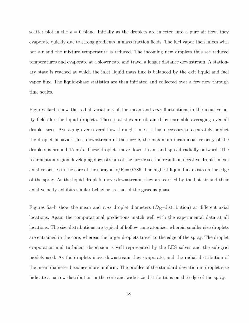
scatter plot in the z = 0 plane. Initially as the droplets are injected into a pure air flow, they

evaporate quickly due to strong gradients in mass fraction fields. The fuel vapor then mixes with

hot air and the mixture temperature is reduced. The incoming new droplets thus see reduced

temperatures and evaporate at a slower rate and travel a longer distance downstream. A station-

ary state is reached at which the inlet liquid mass flux is balanced by the exit liquid and fuel

vapor flux. The liquid-phase statistics are then initiated and collected over a few flow through

time scales.

Figures 4a–b show the radial variations of the mean and rms fluctuations in the axial veloc-

ity fields for the liquid droplets. These statistics are obtained by ensemble averaging over all

droplet sizes. Averaging over several flow through times is thus necessary to accurately predict

the droplet behavior. Just downstream of the nozzle, the maximum mean axial velocity of the

droplets is around 15 m/s. These droplets move downstream and spread radially outward. The

recirculation region developing downstream of the nozzle section results in negative droplet mean

axial velocities in the core of the spray at x/R = 0.786. The highest liquid flux exists on the edge

of the spray. As the liquid droplets move downstream, they are carried by the hot air and their

axial velocity exhibits similar behavior as that of the gaseous phase.

Figures 5a–b show the mean and rms droplet diameters (D10–distribution) at different axial

locations. Again the computational predictions match well with the experimental data at all

locations. The size distributions are typical of hollow cone atomizer wherein smaller size droplets

are entrained in the core, whereas the larger droplets travel to the edge of the spray. The droplet

evaporation and turbulent dispersion is well represented by the LES solver and the sub-grid

models used. As the droplets move downstream they evaporate, and the radial distribution of

the mean diameter becomes more uniform. The profiles of the standard deviation in droplet size

indicate a narrow distribution in the core and wide size distributions on the edge of the spray.

18

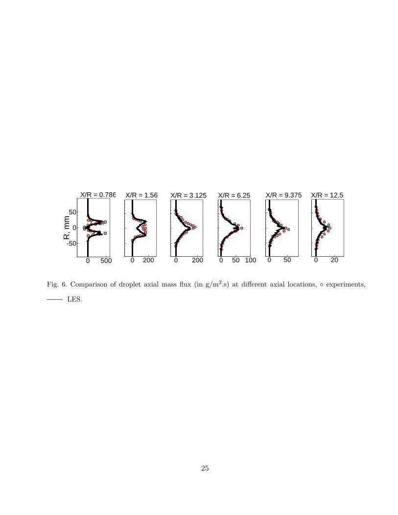
Finally, figure 6 shows the variation in the droplet axial mass flux at different axial locations. The

maximum axial flux decreases as we move in the downstream direction indicating evaporation.

Again good agreement is obtained at all locations. Again two peaks characterizing the hollow

cone spray is visible. These peak spread radially making roughly a 60◦ cone angle. Further

downstream, the spreading of the spray is hindered by the entrainment of the annular air jet and

the maximum mass-flux shifts to the core region.

6 Summary and Conclusions

A large-eddy simulation of evaporating liquid spray in a model coaxial combustor was performed

under the under conditions corresponding to an experiment by Sommerfeld & Qiu [15]. The vari-

able density, low-Mach number equations for non-reacting turbulent flows with phase change due

to droplet evaporation are solved on an unstructured hexahedral mesh. The droplet dynamics is

modeled using the point-particle approach and a uniform state equilibrium model for evapora-

tion. Good agreement with available experimental data for the mean and standard deviations in

the velocity and droplet size throughout the domain was obtained. The only input to the simula-

tion was the size-velocity correlations for liquid droplets at the inlet section, the mass flow rates

and fluid properties. It was shown that with well prescribed boundary conditions, the present

LES formulation together with the Lagrangian particle tracking captures the droplet dispersion

characteristics accurately. In the present study, however, the droplet evaporation was primarily

governed by mass-diffusion. The vapor mass-fractions in the surrounding fluid are considerably

lower than those at the droplet surface. The influence of droplet evaporation on scalar dissipa-

tion rates and mixture fraction variance was not pronounced. The present formulation together

with advanced models for micro-mixing can be used to simulate turbulent spray combustion in

realistic configurations.

19

Acknowledgments

Support for this work was provided by the United States Department of Energy under the

Advanced Scientific Computing (ASC) program. We are indebted to Dr. Gianluca Iaccarino and

Dr. Joseph Oefelein for their help at various stages of this study.

References

[1] Mahesh, K.. Constantinescu, G., and Moin, P., J. Comp. Phy., 197:215–240 (2004).

[2] Elghobashi, S., Appl. Sci. Res. 52:309–329, (1984).

[3] Reade, W. C. and Collins, L. R. Phys. Fluids 12:2530–2540, (2000).

[4] Rouson, D. W. I. and Eaton, J. K. J. Fluid Mech. 348:149–169, (2001).

[5] Wang, Q. and Squires, K.D., Phy. Fluids, 8:1207–1223, (1996).

[6] Apte, S. V., Mahesh, K., Moin, P., and Oefelein, J.C., Int. J. Mult. Flow 29:1311–1331 (2003a).

[7] Sommerfeld, M., Ando, A., and Qiu, H. H. J. Fluids. Engr., 114:648–656 (1992).

[8] Pozorski, J., and Apte, S.V.., Int. J. Mult. Flow, accepted pending revisions, 2008.

[9] Fede, P., Simonin, O., Villedieu, P., and Squires, K.D., Proc. Summer Program, Center for

Turbulence Research, Stanford University, (2006).

[10] O’Kongo, N., and Bellan, J. J. Fluid Mech, 499:1–47, (2004)

[11] Reveillon, J., and Vervisch, L. Comb. Flame, 121:75–90 (2000).

[12] Apte, S. V., Gorokhovski, M., and Moin, P., Int. J. Mult. Flow 29:1503–1522 (2003b).

[13] Patel, N., Kirtas, M., Sankaran, V., and Menon, S, Proc. Comb. Inst., 31:2327–2334 (2007).

20

[14] Mahesh, K., Constantinescu, G., Apte, S.V., Iaccarino, G., Ham, F., and Moin, P., ASME J. App.

Mech., 7:374–381 (2006).

[15] Sommerfeld, M., and Qiu, H.H., Int. J. Heat Fluid Flow, 19:10–22 (1998).

[16] Chen, X. Q., and Pereira, J. C. F., Int. J. Heat Mass Transfer 39:441 (1996).

[17] Liu, Z., Zheng, C., and Zhou, L., Proc. Comb. Inst. 29:561–568 (2002).

[18] Moin, P., Squires, K., Cabot, W., and Lee, S., Phy. Fluid A., 3:2746–1757 (1991).

[19] Pierce, C. and Moin, P., Phy. Fluids, 10:2041–3044 (1998).

[20] Crowe, C., Sommerfeld, M., and Tsuji, Y. Multiphase flows with droplets, and particles, CRC Press

(1998).

[21] Apte, S. V., Mahesh, K., and Lundgren, T., Int. J. Mult. Flow 34: 260–271 (2008).

[22] Faeth, G., Prog. Energy Combust. Sci., 9:1–76 (1998).

[23] Law, C.K., Prog. Energy Combust. Sci. 8:171 (1982).

[24] Sirignano, W. M., Fluid Dynamics and Transport of Droplets and Sprays, Cambridge University

Press, Cambridge, 1999.

[25] Miller, R., Harstad, K., and Bellan, J., Int. J. Mult. Flow, 24:1025–1055 (1998).

[26] Masoudi, M., and Sirignano, W.A. Int. J. Mult. Flow, 27: 1707–1734, 2001.

[27] Oefelein, J. C., Simulation and analysis of turbulent multiphase combustion processes at high

pressures, Ph.D. Thesis, The Pennsylvania State University, University Park, Pa, 1997.

[28] Pierce, C.D., and Moin, P., AIAA J., 36:1325–1327 (1998).

21

List of Figures

1 Schematic diagram of the computational domain for model combustor of

Sommerfeld & Qiu [15]. 23

2 Close-up of the computational grid: (a) x–y plane, (b) y–z. 23

3 Instantaneous snapshot of fuel mass-fraction and liquid droplets in the z = 0

plane. 23

4 Comparison of mean and rms axial velocity averaged over all droplet sizes at

different axial locations: (a) u, (b) u′ in m/s, ◦ experiments, LES. 24

5 Comparison of mean and rms droplet diameters averaged over all droplet sizes

at different axial locations: (a) dp, (b) d′p in µm, ◦ experiments, LES. 24

6 Comparison of droplet axial mass flux (in g/m2.s) at different axial locations, ◦

experiments, LES. 25

22

Fig. 1. Schematic diagram of the computational domain for model combustor of Sommerfeld & Qiu [15].

Fig. 2. Close-up of the computational grid: (a) x–y plane, (b) y–z.

Fig. 3. Instantaneous snapshot of fuel mass-fraction and liquid droplets in the z = 0 plane.

23

R,m

m

0 1 2 3

-50

0

50

0 2 4 0 2 4 0 2 4 0 2 4 0 2 4

(b)

R,m

m

0 10 20

-50

0

50

X/R = 0.786

0 10 20

X/R = 1.56

0 10 20

X/R = 3.125

0 10 20

X/R = 6.25

0 10 20

X/R = 9.375

0 10 20

X/R = 12.5(a)

Fig. 4. Comparison of mean and rms axial velocity averaged over all droplet sizes at different axial

locations: (a) u, (b) u′ in m/s, ◦ experiments, LES.

R,m

m

0 50 100

-50

0

50

X/R=0.781

0 50 100

X/R=1.56

10 20 30 40

(a)X/R=12.5

20 30 40

X/R=9.375

20 30 40 50

X/R=6.25

20 40 60

X/R=3.125

0 10 200 10 200 20 400 20 40

R,m

m

0 20 40

-50

0

50

0 10 20

(b)

Fig. 5. Comparison of mean and rms droplet diameters averaged over all droplet sizes at different axial

locations: (a) dp, (b) d′p in µm, ◦ experiments, LES.

24

0 200

X/R = 3.125

0 50 100

X/R = 6.25

0 50

X/R = 9.375

R,m

m

0 500

-50

0

50

X/R = 0.786

0 200

X/R = 1.56

0 20

X/R = 12.5

Fig. 6. Comparison of droplet axial mass flux (in g/m2.s) at different axial locations, ◦ experiments,

LES.

25