Large Dynamic Range Transverse Beam Profile...

ERL2013, Novosibirsk

Large Dynamic RangeTransverse Beam Profile

Measurements

Pavel EvtushenkoJefferson Lab FEL


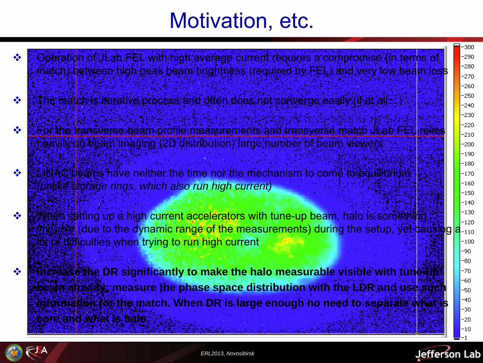
Operation of JLab FEL with high average current requires a compromise (in terms of match) between high peak beam brightness (required by FEL) and very low beam loss

The match is iterative process and often does not converge easily (if at all…)

For the transverse beam profile measurements and transverse match JLab FEL relies heavily on beam imaging (2D distribution) large number of beam viewers

LINAC beams have neither the time nor the mechanism to come to equilibrium(unlike storage rings, which also run high current)

When setting up a high current accelerators with tune-up beam, halo is something invisible (due to the dynamic range of the measurements) during the setup, yet causing a lot of difficulties when trying to run high current

Increase the DR significantly to make the halo measurable visible with tune-up beam already; measure the phase space distribution with the LDR and use such information for the match. When DR is large enough no need to separate what is core and what is halo.

Motivation, etc.


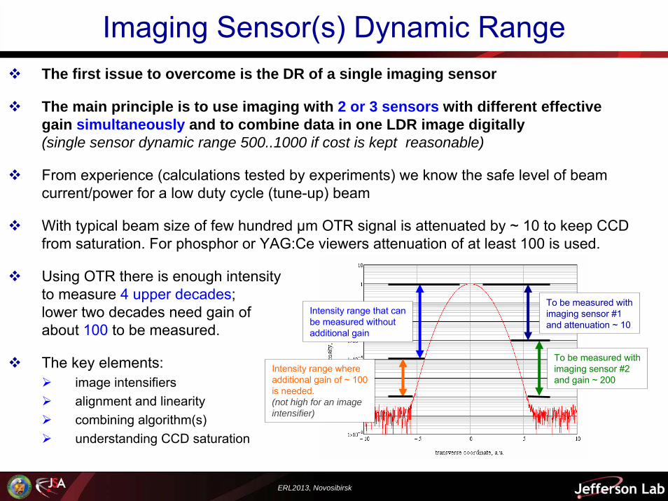
Imaging Sensor(s) Dynamic RangeThe first issue to overcome is the DR of a single imaging sensor

The main principle is to use imaging with 2 or 3 sensors with different effective gain simultaneously and to combine data in one LDR image digitally(single sensor dynamic range 500..1000 if cost is kept reasonable)

From experience (calculations tested by experiments) we know the safe level of beam current/power for a low duty cycle (tune-up) beam

With typical beam size of few hundred μm OTR signal is attenuated by ~ 10 to keep CCD from saturation. For phosphor or YAG:Ce viewers attenuation of at least 100 is used.

Using OTR there is enough intensityto measure 4 upper decades;lower two decades need gain ofabout 100 to be measured.

The key elements:image intensifiersalignment and linearitycombining algorithm(s)understanding CCD saturation

Intensity range that canbe measured without additional gain

Intensity range whereadditional gain of ~ 100is needed.(not high for an imageintensifier)

To be measured withimaging sensor #1and attenuation ~ 10

To be measured withimaging sensor #2and gain ~ 200


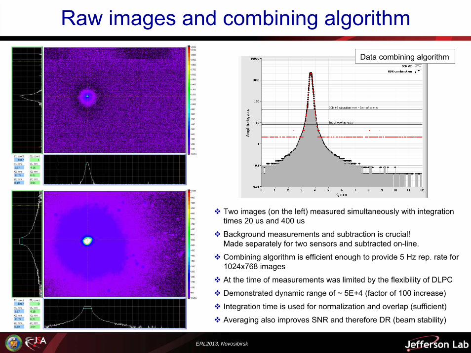
Raw images and combining algorithm

Two images (on the left) measured simultaneously with integration times 20 us and 400 us

Background measurements and subtraction is crucial!Made separately for two sensors and subtracted on-line.

Combining algorithm is efficient enough to provide 5 Hz rep. rate for 1024x768 images

At the time of measurements was limited by the flexibility of DLPC

Demonstrated dynamic range of ~ 5E+4 (factor of 100 increase)

Integration time is used for normalization and overlap (sufficient)

Averaging also improves SNR and therefore DR (beam stability)

Data combining algorithm


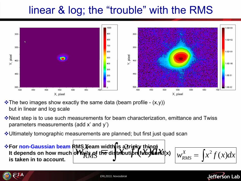
linear & log; the “trouble” with the RMS

The two images show exactly the same data (beam profile - (x,y))but in linear and log scale

Next step is to use such measurements for beam characterization, emittance and Twissparameters measurements (add x’ and y’)

Ultimately tomographic measurements are planned; but first just quad scan

∫= dxxfxwXRMS )(2

For non-Gaussian beam RMS beam width is a tricky thing!It depends on how much of tails of the distribution function f(x)is taken in to account. ∫= dxxfxwX

RMS )(2


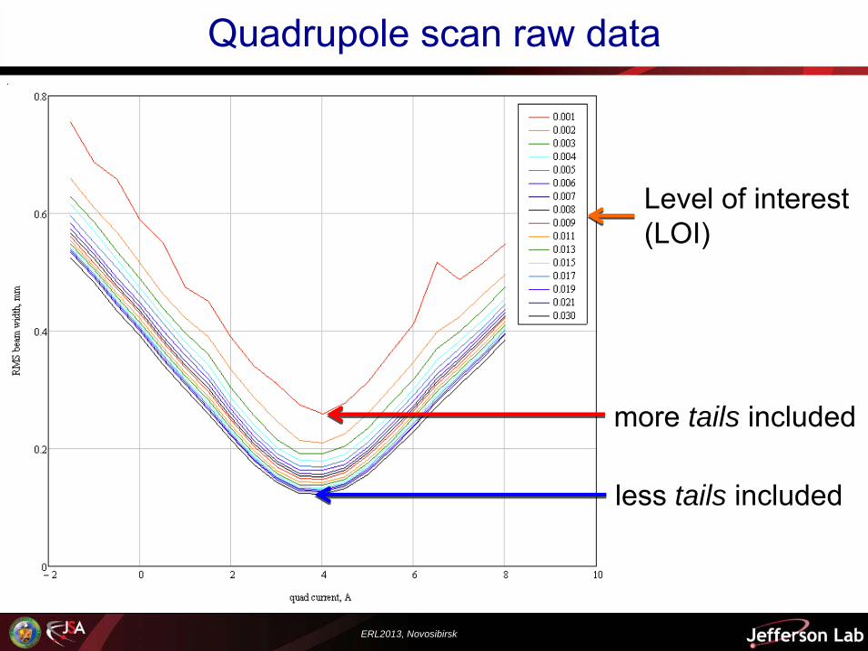
Quadrupole scan raw data

Level of interest(LOI)

more tails included

less tails included


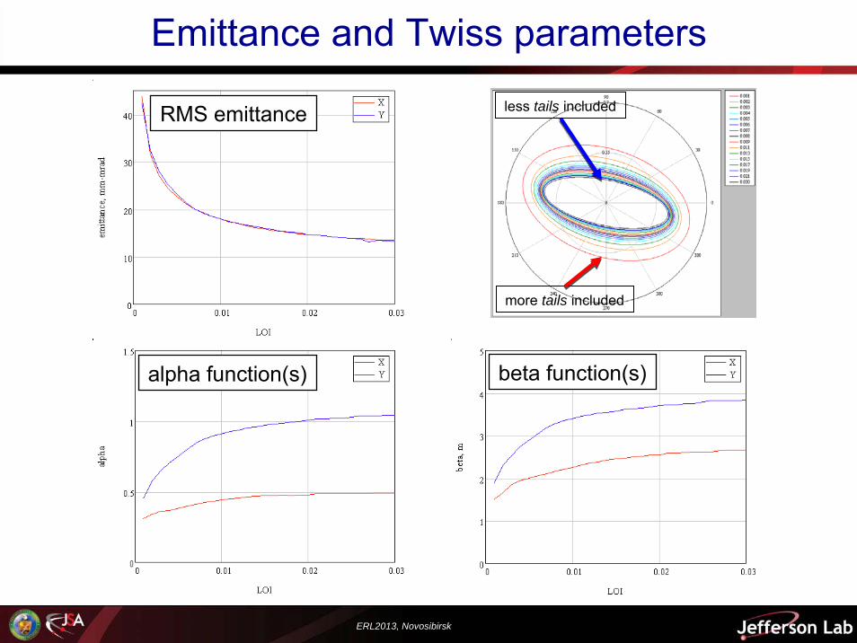
Emittance and Twiss parameters

beta function(s) alpha function(s)

RMS emittance

more tails included

less tails included


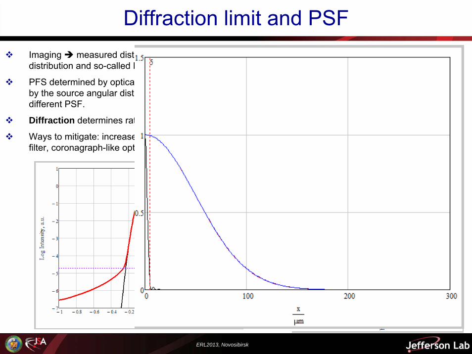
Diffraction limit and PSFImaging measured distribution is a convolution of source distribution and so-called Point Spread Function (PSF)

PFS determined by optical system angular acceptance but also by the source angular distribution. Different beam viewers have different PSF.

Diffraction determines rather hard limits to the DR

Ways to mitigate: increase angular acceptance, use spatial filter, coronagraph-like optics


Objective Lens Pupil ApodizationFirst a Lyot’s coronagraph was considered to improve the PSF, but this would not allow for simultaneous measurements of the beam core and halo, but it is a good exercise

Domain of Fourier optic, always Fresnel approximation – numerical calculations required for most of the interesting cases – becomes demanding on CPU and memory quickly due to large apertures and optical wavelength (~ 0.5 um)

Implemented and used quasi-discrete Hankel transform for optics modeling (allows to do 1D calculations vs. 2D)

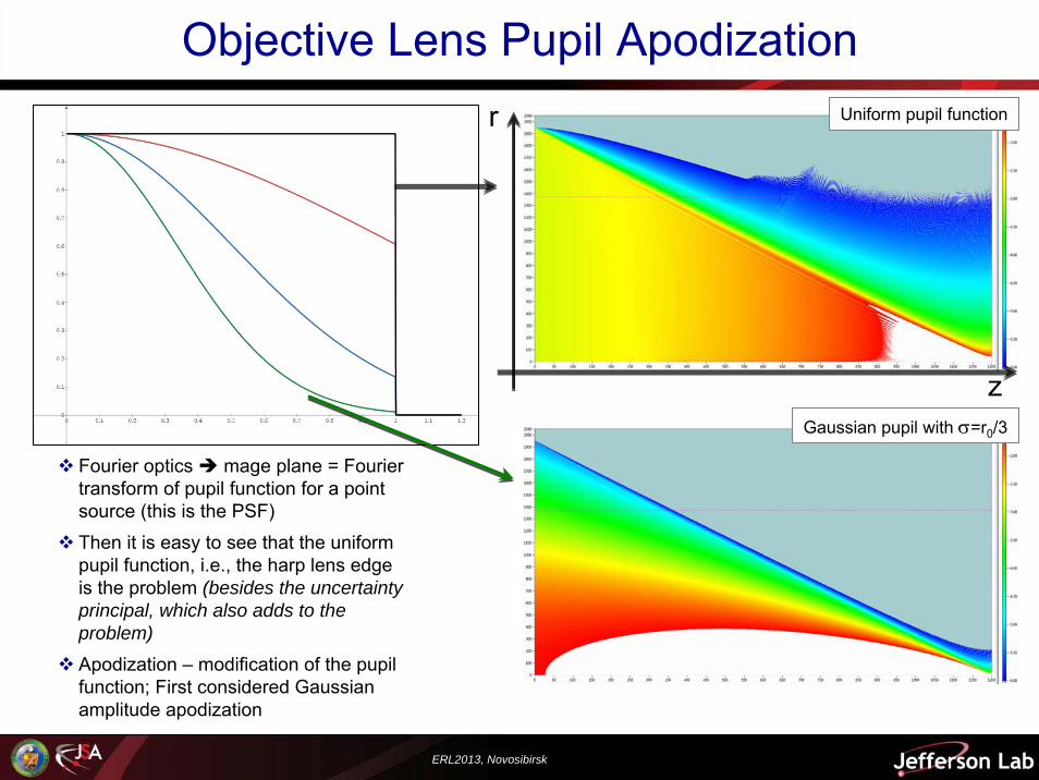
Fourier optics mage plane = Fourier transform of pupil function for a point source (this is the PSF)

Then it is easy to see that the uniform pupil function, i.e., the harp lens edgeis the problem (besides the uncertainty principal, which also adds to the problem)

Apodization – modification of the pupil function; First considered Gaussian amplitude apodization

optical field propagation by means of qDHT(false colors – intensity in log scale)

r

z

Uniform pupil function

Gaussian pupil with σ=r0/3


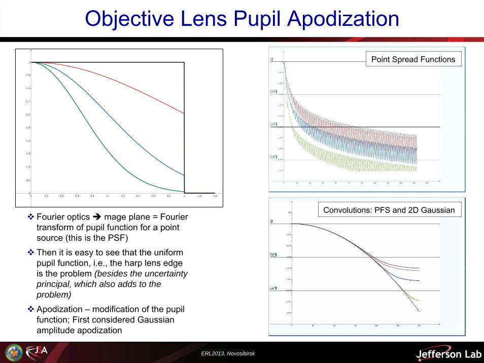
Objective Lens Pupil Apodization

Point Spread Functions

Convolutions: PFS and 2D Gaussian

First a Lyot’s coronagraph was considered to improve the PSF, but this would not allow for simultaneous measurements of the beam core and halo, but it is a good exercise

Domain of Fourier optic, always Fresnel approximation – numerical calculations required for most of the interesting cases – becomes demanding on CPU and memory quickly due to large apertures and optical wavelength (~ 0.5 um)

Implemented and used quasi-discrete Hankel transform for optics modeling (allows to do 1D calculations vs. 2D)

Fourier optics mage plane = Fourier transform of pupil function for a point source (this is the PSF)

Then it is easy to see that the uniform pupil function, i.e., the harp lens edgeis the problem (besides the uncertainty principal, which also adds to the problem)

Apodization – modification of the pupil function; First considered Gaussian amplitude apodization


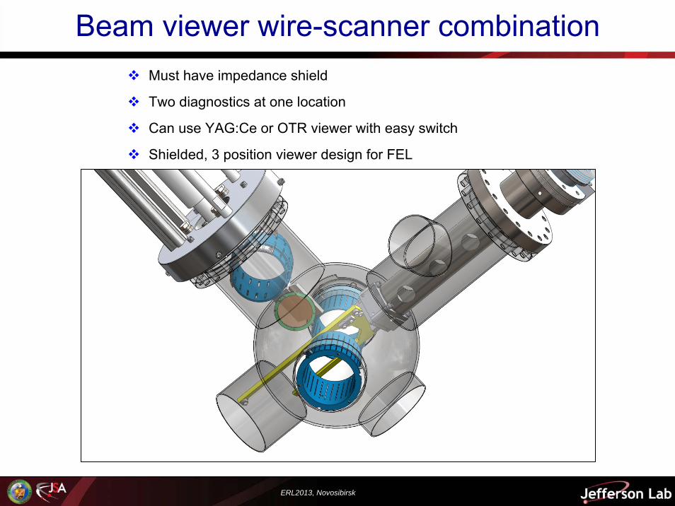
Beam viewer wire-scanner combinationMust have impedance shield

Two diagnostics at one location

Can use YAG:Ce or OTR viewer with easy switch

Shielded, 3 position viewer design for FEL


In conclusion

we have demonstrated beam imaging with DR increased by ~ 100

applied the LDR imaging to beam characterization and have shown that for LINAC non-Gaussian beam the DR has strong impact on the measurements results

have modeled optics required to improve the DR range to reach 106

new diagnostic station for LDR imaging and cross-check with wire scanner was designed and built

next1 - practical implementation of the apodization optics (manufacturing, error sensitivity study, optimization)

next2 - beam measurements with new diagnostics (tomographicphase space measurements based on LDR imaging)

Large Dynamic Range Transverse Beam Profile...

Documents

Transcript of Large Dynamic Range Transverse Beam Profile...