Laplacian Dynamics on General Graphs - Home of …vcp.med.harvard.edu/papers/jg-lap-dyn.pdf ·...
32
Bull Math Biol DOI 10.1007/s11538-013-9884-8 ORIGINAL ARTICLE Laplacian Dynamics on General Graphs Inomzhon Mirzaev · Jeremy Gunawardena Received: 13 May 2013 / Accepted: 23 July 2013 © Society for Mathematical Biology 2013 Abstract In previous work, we have introduced a “linear framework” for time-scale separation in biochemical systems, which is based on a labelled, directed graph, G, and an associated linear differential equation, dx/dt = L(G) · x , where L(G) is the Laplacian matrix of G. Biochemical nonlinearity is encoded in the graph labels. Many central results in molecular biology can be systematically derived within this frame- work, including those for enzyme kinetics, allosteric proteins, G-protein coupled re- ceptors, ion channels, gene regulation at thermodynamic equilibrium, and protein post-translational modification. In the present paper, in response to new applications, which accommodate nonequilibrium mechanisms in eukaryotic gene regulation, we lay out the mathematical foundations of the framework. We show that, for any graph and any initial condition, the dynamics always reaches a steady state, which can be algorithmically calculated. If the graph is not strongly connected, which may occur in gene regulation, we show that the dynamics can exhibit flexible behavior that resem- bles multistability. We further reveal an unexpected equivalence between determin- istic Laplacian dynamics and the master equations of continuous-time Markov pro- cesses, which allows rigorous treatment within the framework of stochastic, single- molecule mechanisms. Keywords Time-scale separation · Linear framework · Graph Laplacian · Matrix-Tree theorem · Gene regulation · Nonequilibrium mechanisms · Markov process · Master equation I. Mirzaev Applied Mathematics Graduate Program, University of Colorado, Boulder, CO, USA e-mail: [email protected] J. Gunawardena (B ) Department of Systems Biology, Harvard Medical School, 200 Longwood Avenue, Boston, MA 02115, USA e-mail: [email protected]
Transcript of Laplacian Dynamics on General Graphs - Home of …vcp.med.harvard.edu/papers/jg-lap-dyn.pdf ·...
Bull Math BiolDOI 10.1007/s11538-013-9884-8
O R I G I NA L A RT I C L E
Laplacian Dynamics on General Graphs
Inomzhon Mirzaev · Jeremy Gunawardena
Received: 13 May 2013 / Accepted: 23 July 2013© Society for Mathematical Biology 2013
Abstract In previous work, we have introduced a “linear framework” for time-scaleseparation in biochemical systems, which is based on a labelled, directed graph, G,and an associated linear differential equation, dx/dt = L(G) · x, where L(G) is theLaplacian matrix of G. Biochemical nonlinearity is encoded in the graph labels. Manycentral results in molecular biology can be systematically derived within this frame-work, including those for enzyme kinetics, allosteric proteins, G-protein coupled re-ceptors, ion channels, gene regulation at thermodynamic equilibrium, and proteinpost-translational modification. In the present paper, in response to new applications,which accommodate nonequilibrium mechanisms in eukaryotic gene regulation, welay out the mathematical foundations of the framework. We show that, for any graphand any initial condition, the dynamics always reaches a steady state, which can bealgorithmically calculated. If the graph is not strongly connected, which may occur ingene regulation, we show that the dynamics can exhibit flexible behavior that resem-bles multistability. We further reveal an unexpected equivalence between determin-istic Laplacian dynamics and the master equations of continuous-time Markov pro-cesses, which allows rigorous treatment within the framework of stochastic, single-molecule mechanisms.
Keywords Time-scale separation · Linear framework · Graph Laplacian ·Matrix-Tree theorem · Gene regulation · Nonequilibrium mechanisms · Markovprocess · Master equation
I. MirzaevApplied Mathematics Graduate Program, University of Colorado, Boulder, CO, USAe-mail: [email protected]
J. Gunawardena (B)Department of Systems Biology, Harvard Medical School, 200 Longwood Avenue, Boston,MA 02115, USAe-mail: [email protected]
I. Mirzaev, J. Gunawardena
1 Introduction
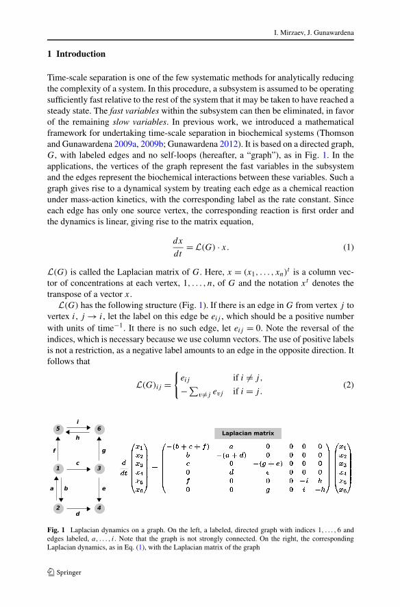
Time-scale separation is one of the few systematic methods for analytically reducingthe complexity of a system. In this procedure, a subsystem is assumed to be operatingsufficiently fast relative to the rest of the system that it may be taken to have reached asteady state. The fast variables within the subsystem can then be eliminated, in favorof the remaining slow variables. In previous work, we introduced a mathematicalframework for undertaking time-scale separation in biochemical systems (Thomsonand Gunawardena 2009a, 2009b; Gunawardena 2012). It is based on a directed graph,G, with labeled edges and no self-loops (hereafter, a “graph”), as in Fig. 1. In theapplications, the vertices of the graph represent the fast variables in the subsystemand the edges represent the biochemical interactions between these variables. Such agraph gives rise to a dynamical system by treating each edge as a chemical reactionunder mass-action kinetics, with the corresponding label as the rate constant. Sinceeach edge has only one source vertex, the corresponding reaction is first order andthe dynamics is linear, giving rise to the matrix equation,
dx
dt= L(G) · x. (1)
L(G) is called the Laplacian matrix of G. Here, x = (x1, . . . , xn)t is a column vec-
tor of concentrations at each vertex, 1, . . . , n, of G and the notation xt denotes thetranspose of a vector x.
L(G) has the following structure (Fig. 1). If there is an edge in G from vertex j tovertex i, j → i, let the label on this edge be eij , which should be a positive numberwith units of time−1. It there is no such edge, let eij = 0. Note the reversal of theindices, which is necessary because we use column vectors. The use of positive labelsis not a restriction, as a negative label amounts to an edge in the opposite direction. Itfollows that
L(G)ij ={
eij if i �= j,
−∑v �=j evj if i = j .
(2)
Fig. 1 Laplacian dynamics on a graph. On the left, a labeled, directed graph with indices 1, . . . ,6 andedges labeled, a, . . . , i. Note that the graph is not strongly connected. On the right, the correspondingLaplacian dynamics, as in Eq. (1), with the Laplacian matrix of the graph
Laplacian Dynamics on General Graphs
Laplacian matrices were first introduced by Gustav Kirchhoff in his pioneering studyof electrical networks (Kirchhoff 1847) and they have been widely studied underdifferent guises, as discussed below.
The key to applying such a “linear framework” to nonlinear biochemical systemslies in the edge labels, eij , which can be algebraic expressions involving the concen-trations of slow variables and the rate constants of biochemical reactions. In effect,the linear framework trades nonlinear dynamics with simple rate constants for lineardynamics with complex labels. This allows steady states to be calculated and the fastvariables to be eliminated, as in the example discussed below.
Many well-known calculations in molecular and systems biology, which havebeen undertaken by distinct, ad hoc methods, can be systematically derived us-ing this linear framework, as explained in Gunawardena (2012). These include theMichaelis–Menten and King–Altman procedures in enzyme kinetics (Michaelis andMenten 1913; King and Altman 1956; Cornish-Bowden 1995); the Monod–Wyman–Changeux and Koshland–Némethy–Filmer formulas in protein allostery (Monodet al. 1965; Koshland et al. 1966) and models derived from these to study G-proteincoupled receptors (Lean et al. 1980; Kenakin 2005) and ligand-gated ion channels(Colquhoun 2006); and the Ackers–Johnson–Shea (Ackers et al. 1982) and relatedformulas based on the “thermodynamic formalism” (Bintu et al. 2005a, 2005b; Se-gal and Widom 2009; Sherman and Cohen 2012), which have been used to studygene regulation in bacteria (Setty et al. 2003; Kuhlman et al. 2007), yeast (Gertzet al. 2009) and flies (Janssens et al. 2006; Zinzen et al. 2006; Segal et al. 2008;He et al. 2010). More recently, the linear framework has been used to analyze thesteady-state behavior of post-translational modification systems (Thomson and Gu-nawardena 2009a, 2009b; Xu and Gunawardena 2012; Dasgupta et al. 2013).
To introduce the linear framework and provide background for the rest of thepaper, the classical Michaelis–Menten formula provides a convenient example.Michaelis and Menten considered the reaction scheme
S + Ek1�k2
ESk3→ P + E, (3)
in which k1, k2, and k3 are the rate constants for mass-action kinetics. They madethe time-scale separation that the enzyme forms E and ES were fast variables, whilesubstrate S and product P were slow. (The historical details are somewhat different;see Cornish-Bowden 1995.) To apply the linear framework, the following labeled,directed graph G is constructed,
�E �ES�
�k1[S]
k2 + k3(4)
in which the vertices represent the fast variables, E and ES, the edges describe thetransitions between these forms and the labels encode the reactions, along with thecontributions of the slow variables. It can easily be checked that, with this labeling,the Laplacian dynamics on G recapitulates the actual dynamics of E and ES comingfrom the reactions in Eq. (3). At steady state, the fluxes must balance, so that
k1[S][E] = (k2 + k3)[ES], (5)
I. Mirzaev, J. Gunawardena
which gives one equation between the two fast variables. This example is so simplethat it is not necessary to construct the graph G in order to deduce Eq. (5) but, in theabsence of G, the linearity of this steady-state calculation is less obvious. A secondequation between the fast variables comes from observing that enzyme is neithercreated nor destroyed and must therefore obey the conservation law
[E] + [ES] = Etot. (6)
Using Eqs. (5) and (6) to solve for [E] and [ES], we find that
[E] = EtotKM
KM + [S] and [ES] = Etot[S]KM + [S] , (7)
where KM = (k2 +k3)/k1 is the Michaelis–Menten constant. Equation (7) allows thefast variables to be eliminated in favour of the conserved total, Etot, and the quantitiesderived from the labels, such as [S] and KM . The rate of the reaction can now becalculated as
d[P ]dt
= k3[ES] = Vmax[S]KM + [S] ,
where Vmax = k3Etot is the maximal reaction velocity. This is the well-knownMichaelis–Menten formula, in which only the slow variables appear.
The main difference between this calculation and other applications of the frame-work is that the graph G can be far more complicated and the steady state can nolonger be determined by simply balancing two fluxes. Instead, it becomes necessaryto calculate x such that dx/dt = 0 or, equivalently, x is in the kernel of the Lapla-cian: kerL(G) = {x | L(G) · x = 0}. In many applications, it has been found that G
is strongly connected. That is, given any two distinct vertices, i and j , there is a pathin G of directed edges from i to j ,
i = i1 → i2 → ·· · → ik = j.
(Since i and j are arbitrary, there must also be such a path from j to i.) Note thatthe graph in Eq. (4) is strongly connected. When G is strongly connected, it can beshown that the kernel of the Laplacian is one- dimensional,
dim kerL(G) = 1. (8)
This result has been central to previous applications of the linear framework. It isproved in Thomson and Gunawardena (2009a) and reappears in the course of thetreatment here as Proposition 3. It has the following implication. The Laplacian dy-namics may be started with arbitrary concentrations at each vertex, so that there are asmany degrees of freedom initially as there are vertices in the graph. Nevertheless, ifa steady state is reached, all these degrees of freedom are lost except one. This is trueno matter how complex the graph, provided only that it is strongly connected. It isthis collapse in the degrees of freedom which allows elimination of the fast variables.
To obtain formulas, it is necessary to identify a basis element in kerL(G).A canonical element, ρ ∈ kerL(G), may be algorithmically calculated from the graph
Laplacian Dynamics on General Graphs
structure using the Matrix-Tree theorem, which is stated below as Theorem 1. The ρi
are sums of products of labels (i.e.: polynomials in the labels) that are determined bythe structure of G. For G in Eq. (4), if E and ES have the indices 1 and 2, respectively,then ρ1 = k2 + k3 and ρ2 = k1[S].
Any steady state, x ∈ kerL(G), can now be determined in terms of ρ. Accordingto Eq. (8), x = λρ where λ is a scalar. This gives n equations, xi = λρi , for the n + 1unknown quantities, x1, . . . , xn, and λ. The remaining equation comes from the factthat the total concentration of material on the graph is conserved, so that
x1 + · · · + xn = xtot (9)
which is the equivalent of Eq. (6) above. Substituting xi = λρi , gives
λ = xtot
ρ1 + · · · + ρn
,
from which the xi can be calculated as
xi = xtotρi
ρ1 + · · · + ρn
. (10)
This is the equivalent of Eq. (7): the xi have been eliminated in terms of the conservedquantity xtot and the quantities in the labels, which appear through the ρi . The variousformulas and models cited above in different areas of biology, in which time-scaleseparation has been used to simplify systems and calculate properties of interest, canall be deduced from Eq. (10) (Gunawardena 2012).
Up to now, the focus of studies on the linear framework has been on steady-statebehavior in strongly-connected graphs and several foundational questions have notbeen addressed. First, it has been generally assumed that no matter what initial con-dition is chosen, the Laplacian dynamics eventually reaches a steady state. While thisseems intuitively plausible, the dynamical behavior of the Laplacian has not been rig-orously analysed. Second, in some application areas, such as gene regulation or ionchannel activity, the system is stochastic in nature, with the vertices of the graph rep-resenting the states of individual molecules, rather than populations of molecules. Therelationship between the macroscopic, deterministic Laplacian dynamics in Eq. (1)and stochastic dynamics has been treated in an ad hoc manner, but has not been rigor-ously clarified. The present paper reveals an unexpectedly close relationship betweenthese two apparently dissimilar formulations.
A further important issue has emerged in recent application of the framework togene regulation away from thermodynamic equilibrium (Ahsendorf et al. 2013). Thisbecomes particularly significant in eukaryotes where dissipative mechanisms play acentral role, as reviewed in the Discussion. In contrast to previous applications ofthe linear framework, nonstrongly connected graphs emerge in this new context. Forthese, the kernel of the Laplacian need no longer be one-dimensional, and we showhere that this can lead to significant qualitative differences in steady-state behaviorfrom the strongly-connected case.
The present paper is intended to address these foundational issues. Applicationsof the results to gene regulation will appear elsewhere (Ahsendorf et al. 2013).
I. Mirzaev, J. Gunawardena
Two further points are relevant to our general approach. First, the Laplacian dy-namics in Eq. (1) is linear and the behavior of linear systems is well understood.For instance, there are standard methods in linear algebra for calculating solutions ofthe steady-state matrix equation L(G) · x = 0. However, these methods use determi-nants, which have terms with alternating signs, and it is not immediately clear thatthe resulting solutions have the important property of positivity (Thomson and Gu-nawardena 2009b, Supplementary Information). That is, if the rate constants and totalconcentrations are all positive, it is important to confirm that quantities like ρi aboveare also positive. The Matrix-Tree theorem guarantees positivity. In general, the in-terplay between dynamics, algebra, and combinatorics has been highly informativeand that approach is continued here.
Second, matrices of Laplacian type have arisen in both fundamental graph theory(Merris 1994; Chung 1997; Chebotarev and Agaev 2002) and in various applicationareas in physics, engineering, computer science, and economics (Schnakenberg 1976;Pecora and Carroll 1998; Nishikawa and Motter 2010; Chen 1971; Olfati-Saber et al.2007; Chebotarev and Agaev 2009; Bott and Mayberry 1954). While some of thealgebraic results proved here can be found in these other literatures, the present treat-ment is necessary for several reasons. Laplacian dynamics, in the form of the first-order biochemistry represented by Eq. (1), has not been discussed previously. Deter-mining the long-time stability of this dynamics is an important goal of the presentpaper. Laplacian matrices have also been defined for many different types of graphs(undirected, unlabeled, etc.) under different notations, conventions, and normaliza-tions. The treatment given here builds upon previous work (Thomson and Gunawar-dena 2009a, 2009b; Gunawardena 2012), and follows uniform conventions that aregrounded in biochemical kinetics. Other sources often focus on particular kinds ofgraphs, such as strongly-connected ones, and address questions of interest to otherdomains. No restrictions are placed here on the graphs being studied and the focusis on issues of interest to biology. Finally, literature sources that are both completeand accessible to a biological audience have not been found. The treatment givenhere is self-contained and elementary, relying largely on well-known results in linearalgebra. We cite relevant sources when these are known to us but must apologize inadvance if we have inadvertently missed others. We would be pleased to know ofthese. We hope that the present paper will provide a helpful resource and encouragefurther exploitation of the linear framework in different areas of biology.
2 Eigenvalues of the Laplacian
We outline some conventions before embarking on the main results. In applicationsof the linear framework, the labels can be algebraic expressions involving actual bio-chemical rate constants and concentrations of slow variables, as in Eq. (4). It can behelpful to work over a rational function field R(a1, . . . , am) in these other parameters,rather than over R; see, for instance, Thomson and Gunawardena (2009a). Here, forsimplicity, we leave these issues to specific applications and work throughout over R.Labels are therefore taken to be uninterpreted symbols which represent positive realnumbers and have units of time−1. The word “graph” will always mean non-empty,
Laplacian Dynamics on General Graphs
labelled, directed graph with no self-loops. The symbol n will be used genericallyfor the number of vertices in the graph under discussion. I will denote the identitymatrix. Within a matrix multiplication, 1 will denote the all-ones vector; the contextshould make clear whether this is a row vector or a column vector. A subscript willbe added, as in In or 1n, to specify the dimension, when needed.
We recall some well-known facts about linear systems (Hirsch and Smale 1974).Let A be a n × n matrix with entries in the real numbers, Aij ∈ R. The linear matrixequation dx/dt = A · x has the solution
x(t) = exp(At) · x(0),
where x(0) is the initial condition and exp(X) is the matrix exponential
exp(X) = I + X + X2
2+ X3
3.2+ · · · + Xm
m! + · · · . (11)
The exponential can be calculated from the Jordan normal form of A, from which itfollows that the solution, xi(t), is a linear combination, over the complex numbers,of terms of the form
tμ exp(λt). (12)
Here, μ is a nonnegative integer, μ = 0,1, . . . , and λ is an eigenvalue of A. A positivepower of t in Eq. (12) indicates that the eigenvalue λ is repeated. Note that λ maybe complex, λ ∈ C. If so, because A is a real matrix, the complex conjugate, λ̄ =Re(λ) − i Im(λ), is also an eigenvalue of A and the linear combination of terms fromEq. (12) still yields a real function.
Our concern here is what happens to x(t) in the limit as t → ∞. Does the linearsystem tend to a steady-state or oscillate or go off to infinity? If λ is an eigenvaluewith Re(λ) = a and Im(λ) = b, then
exp(λt) = exp(at)(cos(bt) + i sin(bt)
).
Hence, if all the eigenvalues of A satisfy Re(λ) < 0, the negative exponential exp(at)
in each term from Eq. (12) will kill both the corresponding tμ, no matter how largeμ is, and the cos(bt) and sin(bt) functions, so that x = 0 is the unique steady stateand x(t) → 0 as t → ∞. This corresponds to the well-known eigenvalue criterion forstability of a dynamical system (Hirsch and Smale 1974).
On the other hand, if none of the eigenvalues are zero and at least one of themsatisfies Re(λ) ≥ 0, then the system will either oscillate or go off to infinity. Thecorner case occurs when one or more of the eigenvalues is zero, for which a moredelicate analysis is required.
This is particularly relevant to the Laplacian matrix of a graph. We note first aconsequence of the conservation law in Eq. (9). Although that was written for thesteady-state concentrations, the total concentration does not change over time, so that
d
dt
(x1(t) + · · · + xn(t)
) = 0.
I. Mirzaev, J. Gunawardena
This follows from Eq. (2), which implies that
1 ·L(G) = 0. (13)
Equation (13) already indicates that L(G) is not of full rank and, therefore, that zerois an eigenvalue.
To know more about the Laplacian eigenvalues, recall Geršgorin’s theorem forthe columns of a matrix A (Horn and Johnson 1985). The ith Geršgorin disc is thecircular area in the complex plane that is centered on the ith diagonal element andwhose radius is the sum of the absolute values of the remaining elements in the ithcolumn: {
z ∈C | |z − Aii | ≤∑j �=i
|Aij |}.
Geršgorin’s theorem states that each eigenvalue occurs in some Geršgorin disc.
Proposition 1 For any graph G, if λ is an eigenvalue of L(G), then either λ = 0 orRe(λ) < 0.
Proof It follows from Eq. (2) that each Geršgorin disc of L(G) is centered on a neg-ative real number and has the same radius in absolute value. Hence, for any eigen-value λ, either λ = 0 or Re(λ) < 0, as required. �
The limiting behavior of Laplacian dynamics therefore hinges on the zero eigen-value. If this eigenvalue is repeated, then Eq. (12) may yield terms of the form tμ,which go to infinity with t . To illustrate the possibilities, consider the following twomatrices:
A =⎛⎝0 0 0
0 0 00 0 0
⎞⎠ and B =
⎛⎝0 1 0
0 0 10 0 0
⎞⎠ , (14)
in each of which the eigenvalue 0 is repeated three times. For A, exp(At) = I , so thatxA(t) = x(0) and the system remains forever in steady state at its initial condition.For B , it is easy to check by direct calculation using Eq. (11) that
exp(Bt) =⎛⎝1 t t2/2
0 1 t
0 0 1
⎞⎠ , (15)
so that xB(t) → ∞ unless x(0)2 = x(0)3 = 0.Recall that the algebraic multiplicity of the eigenvalue λ, alg(λ), is the number of
times that λ occurs as a repeated root of the characteristic polynomial or, equivalently,the total size of all the Jordan blocks associated to λ in the Jordan normal form. Incontrast, the geometric multiplicity of λ, geo(λ), is simply the number of Jordanblocks associated to λ or, equivalently, the dimension of the λ eigenspace. Evidently,alg(λ) ≥ geo(λ) and, since A and B are already in Jordan normal form, it is easy to
Laplacian Dynamics on General Graphs
check that
algA(0) = 3, geoA(0) = 3 and algB(0) = 3, geoB(0) = 1.
It is the discrepancy between the two multiplicities of B that leads to the unstablebehavior of xB(t), as confirmed by the following result.
Proposition 2 Suppose that the real matrix A has the same eigenvalue distributionas a Laplacian matrix, as given by Proposition 1. If algA(0) = geoA(0), then thesolution of dx/dt = A · x tends to a steady state as t → ∞ for any initial condition,while if algA(0) > geoA(0) then there is some initial condition for which x(t) → ∞.
Proof The proof follows from standard results (Hirsch and Smale 1974) but for thesake of completeness an outline is given here. Consider first the case in which a basishas been chosen so that A is in Jordan normal form,
A =
⎛⎜⎜⎜⎜⎝
A1 0 . . . 0
0 A2 0 0...
.... . . 0
0 . . . 0 Ak
⎞⎟⎟⎟⎟⎠ .
A has diagonal Jordan blocks, A1, . . . ,Ak , each corresponding to some eigenvalueof A. Since matrices can be multiplied in blocks, exp(At) is also block diagonal, withthe corresponding blocks exp(A1t), . . . , exp(Akt). If Ai corresponds to an eigenvalueλ with Re(λ) < 0 and u is any initial condition for Ai , then exp(Ait) · u → 0 ast → ∞. It follows that the behavior of the solution x(t) = exp(At) · x(0) as t → ∞depends only on the blocks corresponding to the eigenvalue 0.
If Ai is such a Jordan block then it has the form of matrix B in Eq. (14), with 0 onthe diagonal, 1 on the super-diagonal and 0 elsewhere, but it can be of any dimension.If algA(0) = geoA(0), then each of the blocks corresponding to the eigenvalue 0 hasdimension 1. By permuting the basis, if necessary, these blocks can be combined intoa single composite block, which now has the form of matrix A in Eq. (14). In thiscase, as above, exp(At) = I and x(t) → c as t → ∞. Evidently, ci = xi(0) if i is anindex in the zero-eigenvalue block and ci = 0 if i is an index outside this block. Italso follows that A · c = 0, so that c is a steady state vector at which dc/dt = 0.
Conversely, if algA(0) > geoA(0) then some block corresponding to the eigen-value 0 has dimension greater than 1. Assume that this block looks like matrix B inEq. (14); the argument is identical for any other size of block. The exponential of thisblock is given in Eq. (15). Let i be the index of the first row and j be the index ofthe last column of this block within matrix A and choose the initial condition x(0) tobe the unit vector in coordinate j . Then (exp(At) · x(0))i = t3, so that x(t) → ∞ ast → ∞, as required.
Finally, if A is any matrix, there is an alternative basis in which it has Jordannormal form. That is, there is an invertible matrix P , such that P −1 · A · P is inJordan normal form. Since exp(P −1 · A · P t) = P −1 · exp(At) · P , the conclusionsreached for the Jordan normal form apply also to A. �
I. Mirzaev, J. Gunawardena
To apply Proposition 2 to Laplacian matrices, it is necessary to exploit the structureof the underlying graph, to which we now turn.
3 Zero Multiplicities for Strongly Connected Graphs
If G is a graph, vertex i is said to ultimately reach vertex j , denoted i ⇒ j , if eitheri = j or there is a path of directed edges from i to j
i = i1 → i2 → ·· · → ik = j.
The relation of ultimate reaching is the reflexive, transitive closure of the edge rela-tion. Vertex i is said to be strongly connected to vertex j , denoted i ≈ j , if i ⇒ j
and j ⇒ i. Strong connectivity is the symmetric closure of ultimate reaching. It is anequivalence relation on the set of vertices, whose equivalence classes are the stronglyconnected components (SCCs) of G. A graph G is strongly connected, in the sensedescribed in Sect. 1, if all of its vertices lie in a single SCC.
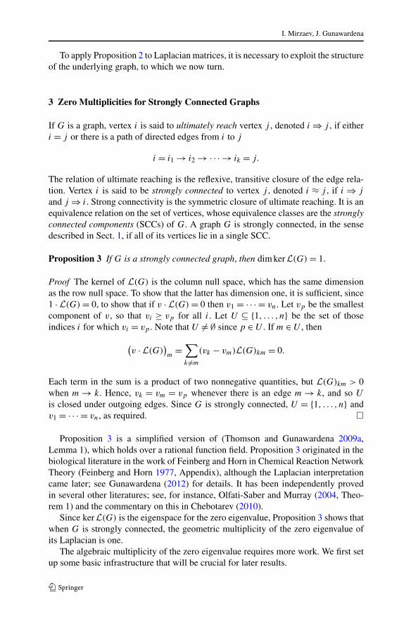
Proposition 3 If G is a strongly connected graph, then dim kerL(G) = 1.
Proof The kernel of L(G) is the column null space, which has the same dimensionas the row null space. To show that the latter has dimension one, it is sufficient, since1 ·L(G) = 0, to show that if v ·L(G) = 0 then v1 = · · · = vn. Let vp be the smallestcomponent of v, so that vi ≥ vp for all i. Let U ⊆ {1, . . . , n} be the set of thoseindices i for which vi = vp . Note that U �= ∅ since p ∈ U . If m ∈ U , then
(v ·L(G)
)m
=∑k �=m
(vk − vm)L(G)km = 0.
Each term in the sum is a product of two nonnegative quantities, but L(G)km > 0when m → k. Hence, vk = vm = vp whenever there is an edge m → k, and so U
is closed under outgoing edges. Since G is strongly connected, U = {1, . . . , n} andv1 = · · · = vn, as required. �
Proposition 3 is a simplified version of (Thomson and Gunawardena 2009a,Lemma 1), which holds over a rational function field. Proposition 3 originated in thebiological literature in the work of Feinberg and Horn in Chemical Reaction NetworkTheory (Feinberg and Horn 1977, Appendix), although the Laplacian interpretationcame later; see Gunawardena (2012) for details. It has been independently provedin several other literatures; see, for instance, Olfati-Saber and Murray (2004, Theo-rem 1) and the commentary on this in Chebotarev (2010).
Since kerL(G) is the eigenspace for the zero eigenvalue, Proposition 3 shows thatwhen G is strongly connected, the geometric multiplicity of the zero eigenvalue ofits Laplacian is one.
The algebraic multiplicity of the zero eigenvalue requires more work. We first setup some basic infrastructure that will be crucial for later results.
Laplacian Dynamics on General Graphs
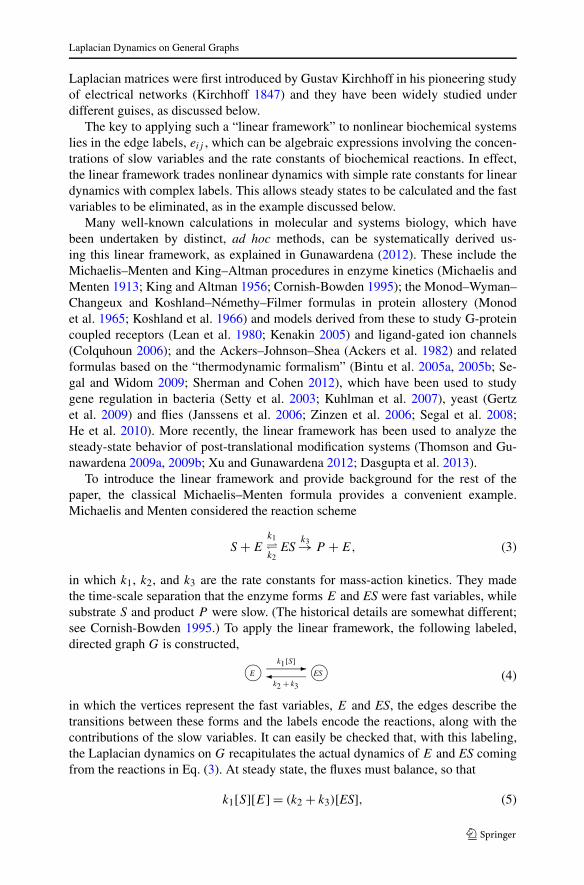
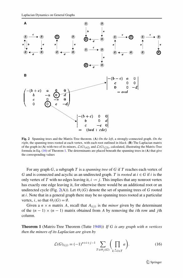
Fig. 2 Spanning trees and the Matrix-Tree theorem. (A) On the left, a strongly-connected graph. On theright, the spanning trees rooted at each vertex, with each root outlined in black. (B) The Laplacian matrixof the graph in (A) with two of its minors, L(G)(42) and L(G)(23) , calculated, illustrating the Matrix-Treeformula in Eq. (16) of Theorem 1. The determinants are placed beneath the spanning trees in (A) that givethe corresponding values
For any graph G, a subgraph T is a spanning tree of G if T reaches each vertex ofG and is connected and acyclic as an undirected graph. T is rooted at i ∈ G if i is theonly vertex of T with no edges leaving it, i � j . This implies that any nonroot vertexhas exactly one edge leaving it, for otherwise there would be an additional root or anundirected cycle (Fig. 2(A)). Let Θi(G) denote the set of spanning trees of G rootedat i. Note that in a general graph there may be no spanning trees rooted at a particularvertex, i, so that Θi(G) = ∅.
Given a n × n matrix A, recall that A(ij) is the minor given by the determinantof the (n − 1) × (n − 1) matrix obtained from A by removing the ith row and j thcolumn.
Theorem 1 (Matrix-Tree Theorem (Tutte 1948)) If G is any graph with n verticesthen the minors of its Laplacian are given by
L(G)(ij) = (−1)n+i+j−1∑
T ∈Θj (G)
( ∏k
a→l∈T
a
). (16)
I. Mirzaev, J. Gunawardena
In other words, up to sign, the (ij)th minor of the Laplacian is the sum, over allspanning trees rooted at j , of the product of the labels on the edges of each tree(Fig. 2(B)). In view of its fundamental importance, a proof of Theorem 1 is given inthe Appendix.
Results of this kind for labeled, directed graphs appear to have been first provedby Tutte (1948); see Moon (1970, Chap. 5) for more background on the mathemat-ical literature. Later authors working in different fields have often rediscovered thisresult without being aware of Tutte’s precedence. For example, the paper of Bottand Mayberry (1954) contains a version of Theorem 1, which has been used in eco-nomics (Whitin 1954), quantum field theory (Jaffe 1965), and statistical mechanics(Schnakenberg 1976). In the biological literature, versions of Theorem 1 were re-discovered by King and Altman in enzyme kinetics (King and Altman 1956) andby Hill in analyzing nonequilibrium biological systems (Hill 1966, 1985). Severalmore powerful variants of the Matrix-Tree theorem are now known, such as theall-minors Matrix-Tree theorem and the Matrix Forest theorem; see Chebotarev andAgaev (2002) for more details.
Lemma 1 A graph G is strongly connected if, and only if, it has a spanning treerooted at each vertex.
Proof Suppose G is strongly connected and choose any vertex i of G. If i is the onlyvertex, then i itself is a spanning tree rooted at i. If not, suppose inductively that a treerooted at i has been constructed and that j is a vertex of G that is not in the tree. SinceG is strongly connected, j ⇒ i and there is some directed path from j to i. Let k bethe first vertex along the path, starting from j , that is a vertex in the tree. The subpathfrom j to k may be added to the tree to form a larger tree in which j is now a vertex.Hence, by induction, there is a tree rooted at i that reaches every vertex. Now supposethat G is a graph. If it has only one vertex, it is strongly connected by definition, sosuppose that it has two distinct vertices i and j . Since there is a spanning tree rootedat i, j must be a vertex on that tree and so j ⇒ i. Similarly, i ⇒ j . Hence, i ≈ j andG is strongly connected. �
If A is a matrix, recall that its adjugate matrix, adj(A) is the transpose of thematrix of cofactors, or signed minors (Horn and Johnson 1985):
adj(A)ij = (−1)i+jA(ji). (17)
Note the reversal of the indices: the ij th entry of the adjugate is, up to sign, the(j i)th minor of A. The adjugate appears in two well known-formulas. The first is theLaplace expansion for the determinant (Horn and Johnson 1985),
adj(A) · A = A · adj(A) = det(A) · I. (18)
If A is the Laplacian matrix of a graph G, then by Proposition 3, detL(G) = 0, andso, by Eq. (17), the columns of adj(L(G)) are elements of kerL(G). Let ρG ∈ R
n>0
denote the column vector given by the spanning trees rooted at each vertex, through
Laplacian Dynamics on General Graphs
the formula in Eq. (16):
ρGi =
∑T ∈Θi(G)
( ∏k
a→l∈T
a
).
Using Eqs. (16) and (17), the adjugate can be expressed in terms of ρG as
adj(L(G)
)ij
= (−1)i+j (−1)n+j+i−1ρGi = (−1)n−1ρG
i . (19)
It follows that each of the columns of adj(L(G)) is, up to sign, equal to ρG. If,moreover, G is strongly connected, then it follows from Lemma 1 that ρG
i > 0 forall i. In particular, ρG �= 0. Since dim kerL(G) = 1 by Proposition 3, this gives abasis for kerL(G).
Corollary 1 If G is a strongly connected graph, then kerL(G) = 〈ρG〉 and ρGi > 0
for all i.
Corollary 1 provides the positivity mentioned in Sect. 1. If the graph is stronglyconnected and the rate constants and concentrations that make up the labels in anyapplication are positive, then ρG has only positive entries.
A second use of the adjugate, which will lead us to the algebraic multiplicity ofthe zero eigenvalue, is the formula for the derivative of a determinant (Magnus andNeudecker 1988, Theorem 8.1),
d
dtdetA(t) = Tr
(adj
(A(t)
) · dA(t)
dt
),
where A(t) is any differentiable matrix function of a single variable. This formulacan be applied, in particular, to the characteristic polynomial of A,
χA(t) = det(A − tI ).
Evaluating the derivative of χA(t) at t = 0 yields
d
dtχA(t)
∣∣t=0 = Tr
(adj(A − tI ) · d
dt(A − tI )
)∣∣∣∣t=0
= Tr(adj(A − tI ) · (−I )
)∣∣t=0
= −Tr(adj(A)
). (20)
Proposition 4 If G is a strongly-connected graph, then algL(G)(0) = 1.
Proof If algL(G)(0) = k, where k ≥ 1, then, by definition of the algebraic multiplic-ity, tk is a factor of χL(G)(t) but tk+1 is not:
χL(G)(t) = tkf (t) where f (0) �= 0.
Accordingly,
d
dtχL(G)(t)
∣∣t=0
{ �= 0 if k = 1,
= 0 if k > 1.(21)
I. Mirzaev, J. Gunawardena
According to Eq. (20), the derivative in question is given by
−(adj11
(L(G)
) + · · · + adjnn
(L(G)
)).
By Eq. (19),
adjii = (−1)n−1ρGi ,
where, by Corollary 1, ρGi > 0 for all i. Hence,
d
dtχL(G)(t)
∣∣t=0 = (−1)n
(ρG
1 + · · · + ρGn
) �= 0.
It follows from Eq. (21) that algL(G)(0) = 1, as required. �
We have established that for a strongly-connected graph, algL(G)(0) =geoL(G)(0) = 1, so that the conditions of Proposition 2 are fulfilled. The extension togeneral graphs can now be undertaken through a structural decomposition of G intoits SCCs.
4 Zero Multiplicities for General Graphs
Let [i] denote the SCC containing i. Given two SCCs, [i] and [j ], [i] is said toprecede [j ], denoted [i] � [j ], if i′ ⇒ j ′ for some i′ ∈ [i] and some j ′ ∈ [j ]. It iseasy to check that this is well defined. The relation of precedes is a partial order onthe SCCs: it is clearly reflexive and transitive and if [i] � [j ] and [j ] � [i] then i
and j are mutually linked by directed paths, so [i] = [j ], and the relation is alsoantisymmetric. It follows that we can distinguish terminal SCCs, which are those [i]such that, if [i] � [j ] then [i] = [j ].
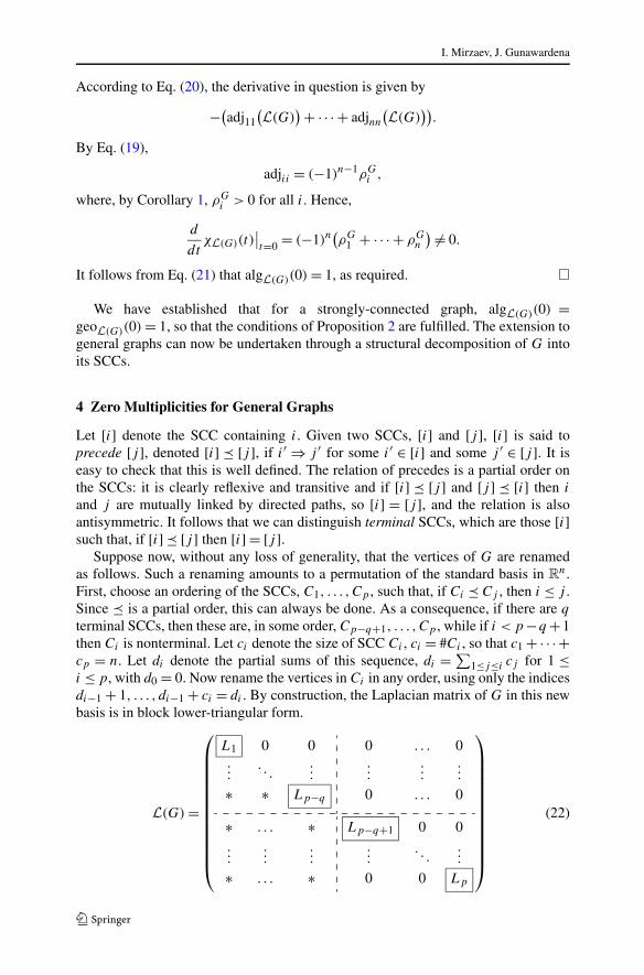
Suppose now, without any loss of generality, that the vertices of G are renamedas follows. Such a renaming amounts to a permutation of the standard basis in R
n.First, choose an ordering of the SCCs, C1, . . . ,Cp , such that, if Ci � Cj , then i ≤ j .Since � is a partial order, this can always be done. As a consequence, if there are q
terminal SCCs, then these are, in some order, Cp−q+1, . . . ,Cp , while if i < p−q +1then Ci is nonterminal. Let ci denote the size of SCC Ci , ci = #Ci , so that c1 + · · ·+cp = n. Let di denote the partial sums of this sequence, di = ∑
1≤j≤i cj for 1 ≤i ≤ p, with d0 = 0. Now rename the vertices in Ci in any order, using only the indicesdi−1 + 1, . . . , di−1 + ci = di . By construction, the Laplacian matrix of G in this newbasis is in block lower-triangular form.
L(G) =
⎛⎜⎜⎜⎜⎜⎜⎜⎜⎜⎜⎜⎜⎝
L1 0 0 0 . . . 0...
. . ....
......
...
∗ ∗ Lp−q 0 . . . 0
∗ . . . ∗ Lp−q+1 0 0...
......
.... . .
...
∗ . . . ∗ 0 0 Lp
⎞⎟⎟⎟⎟⎟⎟⎟⎟⎟⎟⎟⎟⎠
(22)
Laplacian Dynamics on General Graphs
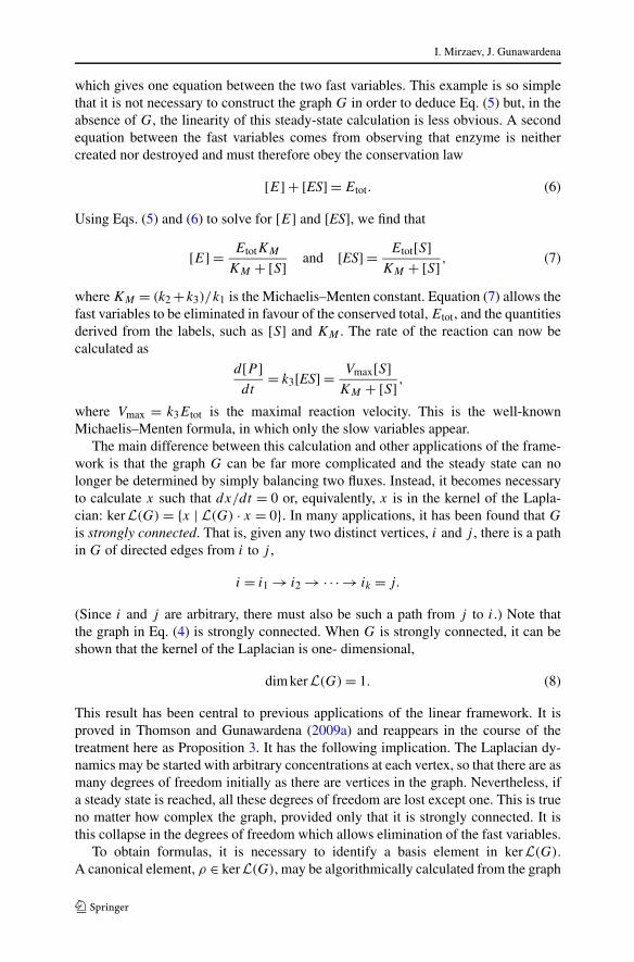
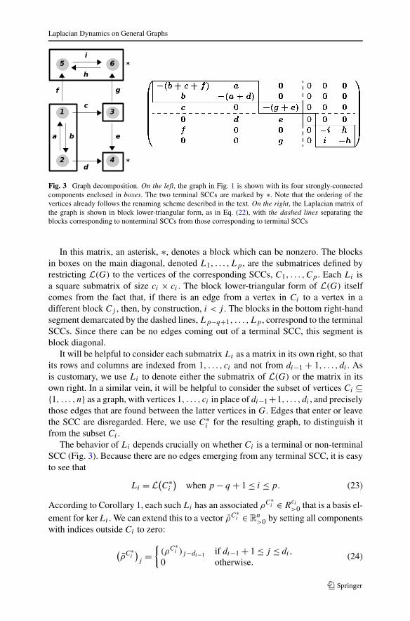
Fig. 3 Graph decomposition. On the left, the graph in Fig. 1 is shown with its four strongly-connectedcomponents enclosed in boxes. The two terminal SCCs are marked by ∗. Note that the ordering of thevertices already follows the renaming scheme described in the text. On the right, the Laplacian matrix ofthe graph is shown in block lower-triangular form, as in Eq. (22), with the dashed lines separating theblocks corresponding to nonterminal SCCs from those corresponding to terminal SCCs
In this matrix, an asterisk, ∗, denotes a block which can be nonzero. The blocksin boxes on the main diagonal, denoted L1, . . . ,Lp , are the submatrices defined byrestricting L(G) to the vertices of the corresponding SCCs, C1, . . . ,Cp . Each Li isa square submatrix of size ci × ci . The block lower-triangular form of L(G) itselfcomes from the fact that, if there is an edge from a vertex in Ci to a vertex in adifferent block Cj , then, by construction, i < j . The blocks in the bottom right-handsegment demarcated by the dashed lines, Lp−q+1, . . . ,Lp , correspond to the terminalSCCs. Since there can be no edges coming out of a terminal SCC, this segment isblock diagonal.
It will be helpful to consider each submatrix Li as a matrix in its own right, so thatits rows and columns are indexed from 1, . . . , ci and not from di−1 + 1, . . . , di . Asis customary, we use Li to denote either the submatrix of L(G) or the matrix in itsown right. In a similar vein, it will be helpful to consider the subset of vertices Ci ⊆{1, . . . , n} as a graph, with vertices 1, . . . , ci in place of di−1 +1, . . . , di , and preciselythose edges that are found between the latter vertices in G. Edges that enter or leavethe SCC are disregarded. Here, we use C∗
i for the resulting graph, to distinguish itfrom the subset Ci .
The behavior of Li depends crucially on whether Ci is a terminal or non-terminalSCC (Fig. 3). Because there are no edges emerging from any terminal SCC, it is easyto see that
Li = L(C∗
i
)when p − q + 1 ≤ i ≤ p. (23)
According to Corollary 1, each such Li has an associated ρC∗i ∈ R
ci
>0 that is a basis el-ement for kerLi . We can extend this to a vector ρ̄C∗
i ∈Rn>0 by setting all components
with indices outside Ci to zero:
(ρ̄C∗
i)j
={
(ρC∗i )j−di−1 if di−1 + 1 ≤ j ≤ di,
0 otherwise.(24)
I. Mirzaev, J. Gunawardena
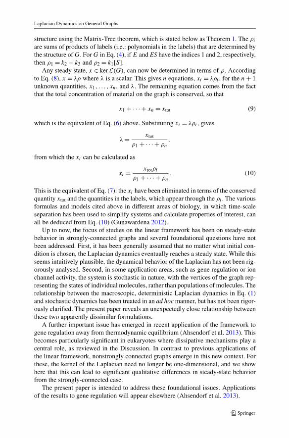
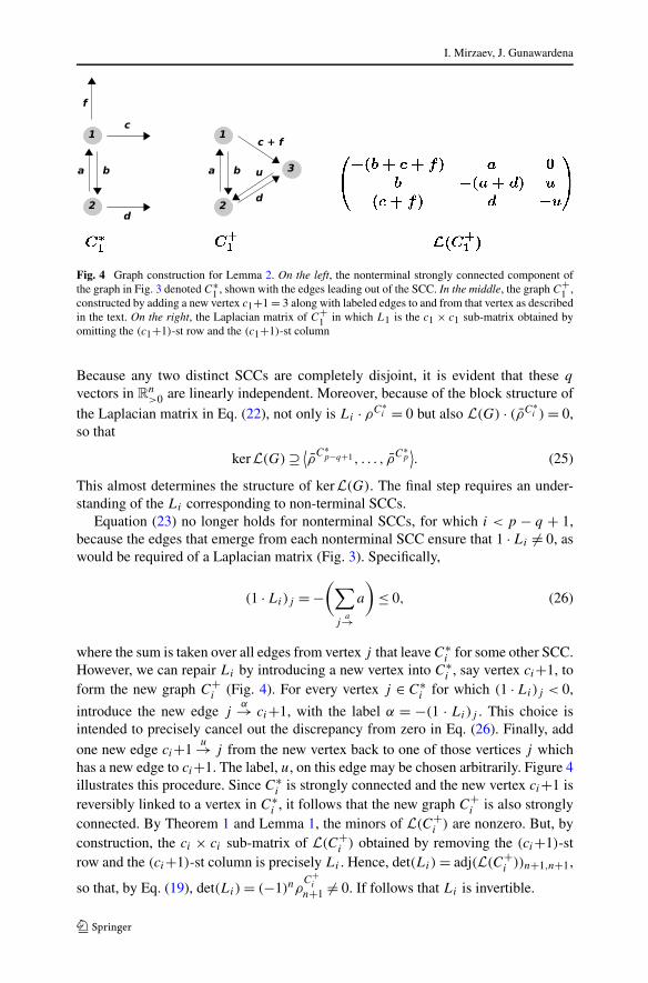
Fig. 4 Graph construction for Lemma 2. On the left, the nonterminal strongly connected component ofthe graph in Fig. 3 denoted C∗
1 , shown with the edges leading out of the SCC. In the middle, the graph C+1 ,
constructed by adding a new vertex c1+1 = 3 along with labeled edges to and from that vertex as describedin the text. On the right, the Laplacian matrix of C+
1 in which L1 is the c1 × c1 sub-matrix obtained byomitting the (c1+1)-st row and the (c1+1)-st column
Because any two distinct SCCs are completely disjoint, it is evident that these q
vectors in Rn>0 are linearly independent. Moreover, because of the block structure of
the Laplacian matrix in Eq. (22), not only is Li · ρC∗i = 0 but also L(G) · (ρ̄C∗
i ) = 0,so that
kerL(G) ⊇ ⟨ρ̄
C∗p−q+1 , . . . , ρ̄C∗
p⟩. (25)
This almost determines the structure of kerL(G). The final step requires an under-standing of the Li corresponding to non-terminal SCCs.
Equation (23) no longer holds for nonterminal SCCs, for which i < p − q + 1,because the edges that emerge from each nonterminal SCC ensure that 1 · Li �= 0, aswould be required of a Laplacian matrix (Fig. 3). Specifically,
(1 · Li)j = −(∑
ja→
a
)≤ 0, (26)
where the sum is taken over all edges from vertex j that leave C∗i for some other SCC.
However, we can repair Li by introducing a new vertex into C∗i , say vertex ci+1, to
form the new graph C+i (Fig. 4). For every vertex j ∈ C∗
i for which (1 · Li)j < 0,
introduce the new edge jα→ ci+1, with the label α = −(1 · Li)j . This choice is
intended to precisely cancel out the discrepancy from zero in Eq. (26). Finally, addone new edge ci+1
u→ j from the new vertex back to one of those vertices j whichhas a new edge to ci+1. The label, u, on this edge may be chosen arbitrarily. Figure 4illustrates this procedure. Since C∗
i is strongly connected and the new vertex ci+1 isreversibly linked to a vertex in C∗
i , it follows that the new graph C+i is also strongly
connected. By Theorem 1 and Lemma 1, the minors of L(C+i ) are nonzero. But, by
construction, the ci × ci sub-matrix of L(C+i ) obtained by removing the (ci+1)-st
row and the (ci+1)-st column is precisely Li . Hence, det(Li) = adj(L(C+i ))n+1,n+1,
so that, by Eq. (19), det(Li) = (−1)nρC+
i
n+1 �= 0. If follows that Li is invertible.
Laplacian Dynamics on General Graphs
Lemma 2 If a graph G is placed in the form required for Eq. (22) then any diagonalblock for a nonterminal SCC is invertible.
With Lemma 2 in hand, the rest is easy. Recall that q is the number of terminalstrongly-connected components of G.
Proposition 5 For any graph G,
kerL(G) = ⟨ρ̄
C∗p−q+1 , . . . , ρ̄C∗
p⟩, (27)
dim kerL(G) = q and geoL(G)(0) = q .
Proof We already know from Eq. (25) that the kerL(G) contains the span of thevectors in Eq. (27). If x ∈ kerL(G), so that L(G) · x = 0, it follows from the blockstructure of the matrix in Eq. (22) and Lemma 2 that xi = 0 for 1 ≤ i ≤ p − q . Sincethe bottom segment of the matrix is block diagonal, x must be in the span of the vec-tors in Eq. (27). This proves Eq. (27) and the other assertions follow immediately. �
Proposition 6 For any graph G, algL(G)(0) = q .
Proof From the block structure of the matrix in Eq. (22), the characteristic polyno-mial of L(G) can be written as the product
χL(G)(t) =p∏
i=1
χLi(t).
For 1 ≤ i ≤ p − q , Li is invertible by Lemma 2, so t does not divide χLi(t). For
p − q + 1 ≤ i ≤ p, each Li is the Laplacian of a strongly-connected graph, so, byProposition 4, t divides χLi
but t2 does not. Hence, tq divides χL(G)(t) but tq+1 doesnot, so that algL(G)(0) = q , as required. �
In the biological literature, dim kerL(G) was first determined for an arbitrarygraph in the work of Feinberg and Horn in Chemical Reaction Network Theory(Feinberg and Horn 1977, Appendix). The description of the basis elements ofkerL(G) using the Matrix-Tree theorem is given in Gunawardena (2012) but the useof Lemma 2, which greatly simplifies the argument, is new. Proposition 5 appears inAgaev and Chebotarev (2000). Proposition 6 is deduced in Chebotarev and Agaev(2002) using a more powerful variant of the Matrix-Tree theorem.
We can finally appeal to Proposition 2 to deduce the result towards which we havebeen working.
Theorem 2 If G is any graph, then the solution of the Laplacian dynamics dx/dt =L(G) · x converges to a steady state as t → ∞, for any initial condition x(0) ∈R
n.
I. Mirzaev, J. Gunawardena
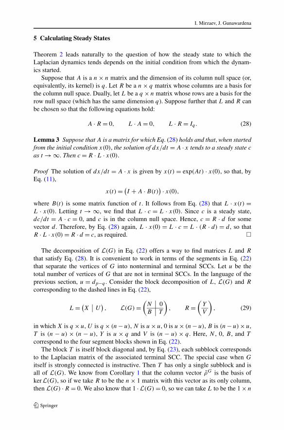
5 Calculating Steady States
Theorem 2 leads naturally to the question of how the steady state to which theLaplacian dynamics tends depends on the initial condition from which the dynam-ics started.
Suppose that A is a n × n matrix and the dimension of its column null space (or,equivalently, its kernel) is q . Let R be a n × q matrix whose columns are a basis forthe column null space. Dually, let L be a q × n matrix whose rows are a basis for therow null space (which has the same dimension q). Suppose further that L and R canbe chosen so that the following equations hold:
A · R = 0, L · A = 0, L · R = Iq . (28)
Lemma 3 Suppose that A is a matrix for which Eq. (28) holds and that, when startedfrom the initial condition x(0), the solution of dx/dt = A · x tends to a steady state c
as t → ∞. Then c = R · L · x(0).
Proof The solution of dx/dt = A · x is given by x(t) = exp(At) · x(0), so that, byEq. (11),
x(t) = (I + A · B(t)
) · x(0),
where B(t) is some matrix function of t . It follows from Eq. (28) that L · x(t) =L · x(0). Letting t → ∞, we find that L · c = L · x(0). Since c is a steady state,dc/dt = A · c = 0, and c is in the column null space. Hence, c = R · d for somevector d . Therefore, by Eq. (28) again, L · x(0) = L · c = L · (R · d) = d , so thatR · L · x(0) = R · d = c, as required. �
The decomposition of L(G) in Eq. (22) offers a way to find matrices L and R
that satisfy Eq. (28). It is convenient to work in terms of the segments in Eq. (22)that separate the vertices of G into nonterminal and terminal SCCs. Let u be thetotal number of vertices of G that are not in terminal SCCs. In the language of theprevious section, u = dp−q . Consider the block decomposition of L, L(G) and R
corresponding to the dashed lines in Eq. (22),
L = (X U
), L(G) =
(N 0B T
), R =
(Y
V
), (29)
in which X is q ×u, U is q × (n−u), N is u×u, 0 is u× (n−u), B is (n−u)×u,T is (n − u) × (n − u), Y is u × q and V is (n − u) × q . Here, N , 0, B , and T
correspond to the four segment blocks shown in Eq. (22).The block T is itself block diagonal and, by Eq. (23), each subblock corresponds
to the Laplacian matrix of the associated terminal SCC. The special case when G
itself is strongly connected is instructive. Then T has only a single subblock and isall of L(G). We know from Corollary 1 that the column vector ρ̄G is the basis ofkerL(G), so if we take R to be the n × 1 matrix with this vector as its only column,then L(G) · R = 0. We also know that 1 ·L(G) = 0, so we can take L to be the 1 × n
Laplacian Dynamics on General Graphs
matrix, which has 1n as its only row. The only issue with this choice of L and R isthat
L · R = 1 · ρ̄G = ρ̄G1 + · · · + ρ̄G
n �= 1,
so that the last requirement in Eq. (28) is not satisfied. However, this is easily reme-died by normalizing R to the total amount in the column, 1 · ρ̄G.
For a general graph G, Proposition 5 provides a specific basis for the column nullspace. Keeping in mind the need for normalization, let R be the n × q matrix whosej th column is given by
R∗j =(
1
1 · ρ̄C∗p−q+j
)ρ̄
C∗p−q+j . (30)
With this choice of R, any row of R whose index is not in a terminal SCC is zero,so that Y = 0, and each column of V has nonzero components only for those indiceswhich are in the corresponding terminal SCC. As for L, Eq. (28) requires that L ·R = In, which by block multiplication requires that U · V = Iq . Accordingly, letU be the q × (n − u) matrix given by first transposing V and then replacing eachnonzero element of V by 1. It is then easy to see that, because of the normalisationof R, U · V = Iq . Moreover, by Eq. (13) applied to each terminal SCC, U · T = 0. Itremains to determine X. Equation (28) requires that L · L(G) = 0, which by blockmultiplication requires that X · N + U · B = 0. We can now appeal once again toLemma 2, which tells us that N is invertible. Hence, we can solve uniquely for X toobtain X = −U · B · N−1. In summary, Eq. (28) is satisfied if
Y = 0, U · T = 0, U · V = I, X = −U · B · N−1. (31)
We deduce from Lemma 3 the following linear relationship between initial conditionsand their resulting steady states.
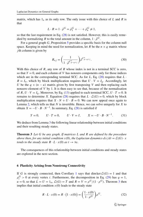
Theorem 3 Let G be any graph. If matrices L and R are defined by the procedureabove then, for any initial condition x(0), the Laplacian dynamics dx/dt = L(G) · xtends to the steady state R · L · x(0) as t → ∞.
The consequences of this relationship between initial conditions and steady statesare explored in the next section.
6 Plasticity Arising from Nonstrong Connectivity
If G is strongly connected, then Corollary 1 says that dim kerL(G) = 1 and thatρG
i > 0 at every vertex i. Furthermore, the decomposition in Eq. (29) has q = 1,u = 0, so that L = U = 1n, L(G) = T and R = V = ρG/(1 · ρG). Theorem 3 thenimplies that initial condition x(0) leads to the steady state
R · L · x(0) = R · (1 · x(0)) =
(1 · x(0)
1 · ρG
)ρG. (32)
I. Mirzaev, J. Gunawardena
The numerator of the scalar factor in Eq. (32) is the conserved quantity, or totalamount of x present initially, 1 · x(0) = xtot, and Eq. (32) corresponds to Eq. (10)in the Introduction. It does not matter on which vertices the initial concentration ofmaterial is placed. No matter how the material is distributed, the steady state that isreached depends only on the total amount that was present. Furthermore, changesin the values of the graph labels may alter the balance of material between differentvertices, but does not cause a qualitative change in the steady-state behavior.
In the general case, where G may no longer be strongly connected, it follows fromTheorem 3 that, if z = L · x(0) ∈ R
q , then the steady state corresponding to x(0) isgiven by the linear combination of the columns of R whose coefficients are the entriesin z. That is, using Eq. (30),
R · L · x(0) = z1
(ρ̄
C∗p−q+1
1 · ρ̄C∗p−q+1
)+ · · · + zq
(ρ̄C∗
p
1 · ρ̄C∗p
). (33)
Since L · L(G) = 0, the rows of the q × n matrix L provide a set of q conserva-tion laws for the Laplacian dynamics, which generalize the single conservation law,1 · L(G) = 0 for the case of a strongly-connected graph. The coefficients z1, . . . , zq
in Eq. (33) are the conserved quantities. Since the columns of R are non-zero onlyon vertices which lie in terminal SCCs, (R · L · x(0))i = 0 for 1 ≤ i ≤ u. For a non-strongly connected graph, no matter what initial condition is chosen, the resultingsteady state is zero on some vertex, indeed, on any vertex that is not in a terminalSCC. Moreover, if k is a vertex in the ith terminal SCC, Cp−q+i , then because theSCCs are pairwise disjoint, the steady state picks out just one of the summands in thelinear combination in Eq. (33):
(R · L · x(0)
)k=
(zi
1 · ρ̄C∗p−q+i
)(ρ̄
C∗p−q+i
)k,
for dp−q+i−1 + 1 ≤ k ≤ dp−q+i . This has a similar form to Eq. (32), with the con-served quantity zi appearing in the numerator of the scalar factor.
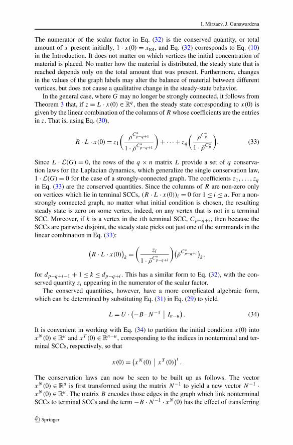
The conserved quantities, however, have a more complicated algebraic form,which can be determined by substituting Eq. (31) in Eq. (29) to yield
L = U · (−B · N−1 In−u
). (34)
It is convenient in working with Eq. (34) to partition the initial condition x(0) intoxN(0) ∈ R
u and xT (0) ∈ Rn−u, corresponding to the indices in nonterminal and ter-
minal SCCs, respectively, so that
x(0) = (xN(0) xT (0)
)t.
The conservation laws can now be seen to be built up as follows. The vectorxN(0) ∈ R
u is first transformed using the matrix N−1 to yield a new vector N−1 ·xN(0) ∈ R
u. The matrix B encodes those edges in the graph which link nonterminalSCCs to terminal SCCs and the term −B · N−1 · xN(0) has the effect of transferring
Laplacian Dynamics on General Graphs
the transformed vector, N−1 · xN(0), into a set of values on the terminal SCCs. Ac-cording to Eq. (34), these values are added to that part of the initial condition thatwas already on the vertices in the terminal SCCs, to form
−B · N−1 · xN(0) + xT (0).
Finally, the matrix U calculates the total value that is now present on each terminalSCC. Recalling the notation used in Eq. (24), the ith conserved quantity in Eq. (33),which corresponds to the ith terminal SCC, Cp−q+i , is given by
zi =dp−q+i∑
k=dp−q+i−1
(−B · N−1 · xN(0) + xT (0))k.
The expression on the right-hand side gives the corresponding conservation law forthe Laplacian dynamics:
d
dt
( dp−q+i∑k=dp−q+i−1
(−B · N−1 · xN(t) + xT (t))k
)= 0.
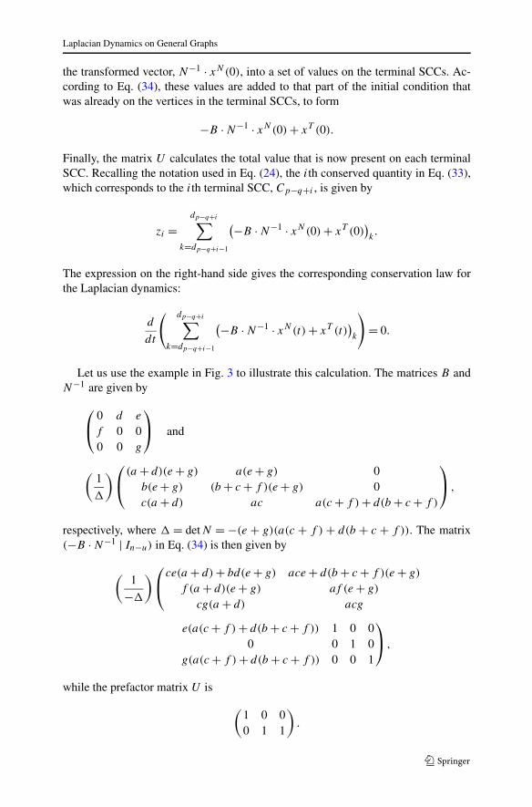
Let us use the example in Fig. 3 to illustrate this calculation. The matrices B andN−1 are given by
⎛⎝ 0 d e
f 0 00 0 g
⎞⎠ and
(1
�
)⎛⎝ (a + d)(e + g) a(e + g) 0
b(e + g) (b + c + f )(e + g) 0c(a + d) ac a(c + f ) + d(b + c + f )
⎞⎠ ,
respectively, where � = detN = −(e + g)(a(c + f ) + d(b + c + f )). The matrix(−B · N−1 | In−u) in Eq. (34) is then given by
(1
−�
)⎛⎝ce(a + d) + bd(e + g) ace + d(b + c + f )(e + g)
f (a + d)(e + g) af (e + g)
cg(a + d) acg
e(a(c + f ) + d(b + c + f )) 1 0 00 0 1 0
g(a(c + f ) + d(b + c + f )) 0 0 1
⎞⎠ ,
while the prefactor matrix U is
(1 0 00 1 1
).
I. Mirzaev, J. Gunawardena
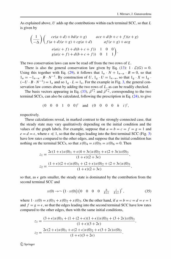
As explained above, U adds up the contributions within each terminal SCC, so that L
is given by
(1
−�
)(ce(a + d) + bd(e + g) ace + d(b + c + f )(e + g)
f (a + d)(e + g) + cg(a + d) af (e + g) + acg
e(a(c + f ) + d(b + c + f )) 1 0 0g(a(c + f ) + d(b + c + f )) 0 1 1
).
The two conservation laws can now be read off from the two rows of L.There is also the general conservation law given by Eq. (13): 1 · L(G) = 0.
Using this together with Eq. (29), it follows that 1u · N + 1n−u · B = 0, so that1u = −1n−u · B · N−1. By construction of U , 1q · U = 1n−u, so that 1q · X = 1q ·(−U · B · N−1) = 1u and so 1q · L = 1n. For the example in Fig. 3, the general con-servation law comes about by adding the two rows of L, as can be readily checked.
The basis vectors appearing in Eq. (33), ρ̄C∗3 and ρ̄C∗
4 , corresponding to the twoterminal SCCs, can also be calculated, following the prescription in Eq. (24), to give
(0 0 0 1 0 0 )t and (0 0 0 0 h i )t ,
respectively.These calculations reveal, in marked contrast to the strongly-connected case, that
the steady state may vary qualitatively depending on the initial condition and thevalues of the graph labels. For example, suppose that a = b = c = f = g = 1 ande = d = ε, where ε � 1, so that the edges leading into the first terminal SCC (Fig. 3)have low rates compared to the other edges, and suppose that the initial condition hasnothing on the terminal SCCs, so that x(0)4 = x(0)5 = x(0)6 = 0. Then
z1 = 2ε(1 + ε)x(0)1 + ε(4 + 3ε)x(0)2 + ε(2 + 3ε)x(0)3
(1 + ε)(2 + 3ε),
z2 = (1 + ε)(2 + ε)x(0)1 + (2 + ε)x(0)2 + (2 + 3ε)x(0)3
(1 + ε)(2 + 3ε),
so that, as ε gets smaller, the steady state is dominated by the contribution from thesecond terminal SCC and
x(0) →∼ (1 · x(0)
) (0 0 0 0 h
h+ii
h+i
)t, (35)
where 1 · x(0) = x(0)1 + x(0)2 + x(0)3. On the other hand, if a = b = c = d = e = 1and f = g = ε, so that the edges leading into the second terminal SCC have low ratescompared to the other edges, then with the same initial conditions,
z1 = (3 + ε)x(0)1 + (1 + (2 + ε)(1 + ε))x(0)2 + (3 + 2ε)x(0)3
(1 + ε)(3 + 2ε),
z2 = 2ε(2 + ε)x(0)1 + ε(2 + ε)x(0)2 + ε(3 + 2ε)x(0)3
(1 + ε)(3 + 2ε).
Laplacian Dynamics on General Graphs
As ε gets smaller, the steady state is dominated by the contribution from the firstterminal SCC and
x(0) →∼ (1 · x(0)
)(0 0 0 1 0 0 )t . (36)
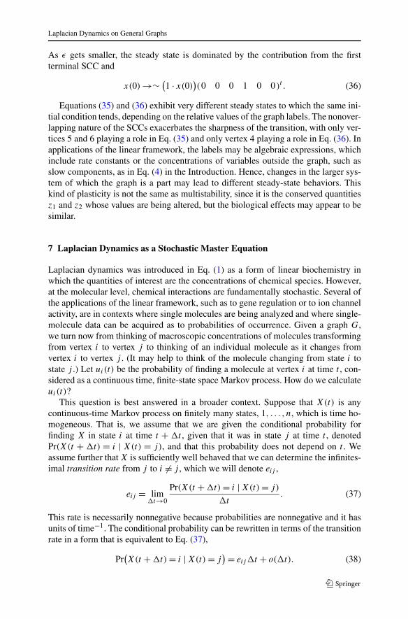
Equations (35) and (36) exhibit very different steady states to which the same ini-tial condition tends, depending on the relative values of the graph labels. The nonover-lapping nature of the SCCs exacerbates the sharpness of the transition, with only ver-tices 5 and 6 playing a role in Eq. (35) and only vertex 4 playing a role in Eq. (36). Inapplications of the linear framework, the labels may be algebraic expressions, whichinclude rate constants or the concentrations of variables outside the graph, such asslow components, as in Eq. (4) in the Introduction. Hence, changes in the larger sys-tem of which the graph is a part may lead to different steady-state behaviors. Thiskind of plasticity is not the same as multistability, since it is the conserved quantitiesz1 and z2 whose values are being altered, but the biological effects may appear to besimilar.
7 Laplacian Dynamics as a Stochastic Master Equation
Laplacian dynamics was introduced in Eq. (1) as a form of linear biochemistry inwhich the quantities of interest are the concentrations of chemical species. However,at the molecular level, chemical interactions are fundamentally stochastic. Several ofthe applications of the linear framework, such as to gene regulation or to ion channelactivity, are in contexts where single molecules are being analyzed and where single-molecule data can be acquired as to probabilities of occurrence. Given a graph G,we turn now from thinking of macroscopic concentrations of molecules transformingfrom vertex i to vertex j to thinking of an individual molecule as it changes fromvertex i to vertex j . (It may help to think of the molecule changing from state i tostate j .) Let ui(t) be the probability of finding a molecule at vertex i at time t , con-sidered as a continuous time, finite-state space Markov process. How do we calculateui(t)?
This question is best answered in a broader context. Suppose that X(t) is anycontinuous-time Markov process on finitely many states, 1, . . . , n, which is time ho-mogeneous. That is, we assume that we are given the conditional probability forfinding X in state i at time t + �t , given that it was in state j at time t , denotedPr(X(t + �t) = i | X(t) = j), and that this probability does not depend on t . Weassume further that X is sufficiently well behaved that we can determine the infinites-imal transition rate from j to i �= j , which we will denote eij ,
eij = lim�t→0
Pr(X(t + �t) = i | X(t) = j)
�t. (37)
This rate is necessarily nonnegative because probabilities are nonnegative and it hasunits of time−1. The conditional probability can be rewritten in terms of the transitionrate in a form that is equivalent to Eq. (37),
Pr(X(t + �t) = i | X(t) = j
) = eij�t + o(�t). (38)
I. Mirzaev, J. Gunawardena
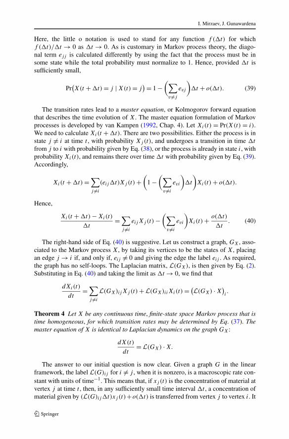
Here, the little o notation is used to stand for any function f (�t) for whichf (�t)/�t → 0 as �t → 0. As is customary in Markov process theory, the diago-nal term ejj is calculated differently by using the fact that the process must be insome state while the total probability must normalize to 1. Hence, provided �t issufficiently small,
Pr(X(t + �t) = j | X(t) = j
) = 1 −(∑
v �=j
evj
)�t + o(�t). (39)
The transition rates lead to a master equation, or Kolmogorov forward equationthat describes the time evolution of X. The master equation formulation of Markovprocesses is developed by van Kampen (1992, Chap. 4). Let Xi(t) = Pr(X(t) = i).We need to calculate Xi(t + �t). There are two possibilities. Either the process is instate j �= i at time t , with probability Xj(t), and undergoes a transition in time �t
from j to i with probability given by Eq. (38), or the process is already in state i, withprobability Xi(t), and remains there over time �t with probability given by Eq. (39).Accordingly,
Xi(t + �t) =∑j �=i
(eij�t)Xj (t) +(
1 −(∑
v �=i
evi
)�t
)Xi(t) + o(�t).
Hence,
Xi(t + �t) − Xi(t)
�t=
∑j �=i
eijXj (t) −(∑
v �=i
evi
)Xi(t) + o(�t)
�t. (40)
The right-hand side of Eq. (40) is suggestive. Let us construct a graph, GX , asso-ciated to the Markov process X, by taking its vertices to be the states of X, placingan edge j → i if, and only if, eij �= 0 and giving the edge the label eij . As required,the graph has no self-loops. The Laplacian matrix, L(GX), is then given by Eq. (2).Substituting in Eq. (40) and taking the limit as �t → 0, we find that
dXi(t)
dt=
∑j �=i
L(GX)ijXj (t) +L(GX)iiXi(t) = (L(GX) · X)
i.
Theorem 4 Let X be any continuous time, finite-state space Markov process that istime homogeneous, for which transition rates may be determined by Eq. (37). Themaster equation of X is identical to Laplacian dynamics on the graph GX :
dX(t)
dt= L(GX) · X.
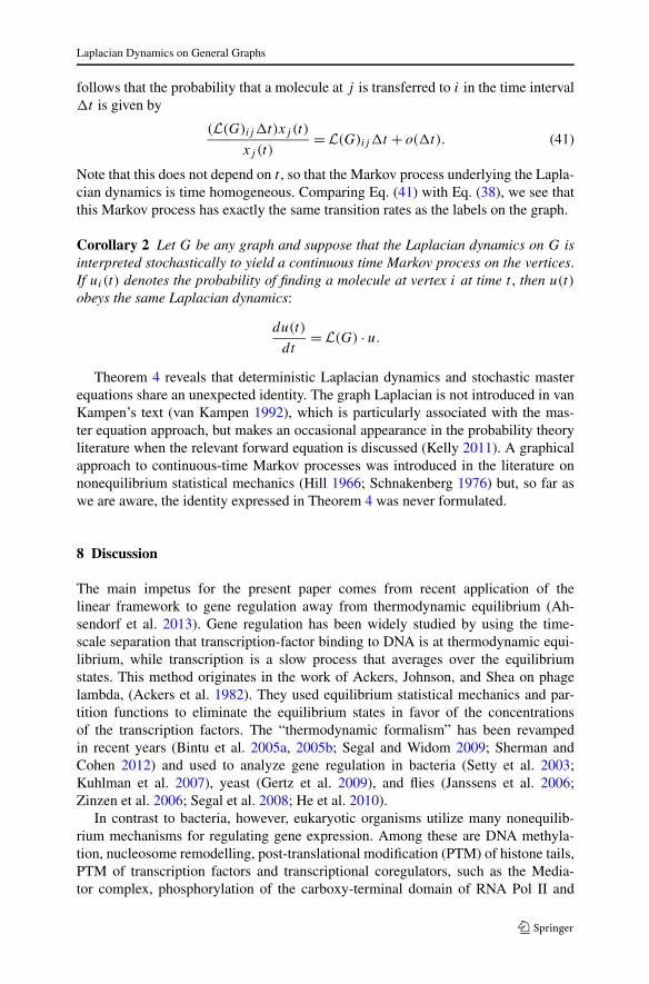
The answer to our initial question is now clear. Given a graph G in the linearframework, the label L(G)ij for i �= j , when it is nonzero, is a macroscopic rate con-stant with units of time−1. This means that, if xj (t) is the concentration of material atvertex j at time t , then, in any sufficiently small time interval �t , a concentration ofmaterial given by (L(G)ij�t)xj (t)+o(�t) is transferred from vertex j to vertex i. It
Laplacian Dynamics on General Graphs
follows that the probability that a molecule at j is transferred to i in the time interval�t is given by
(L(G)ij�t)xj (t)
xj (t)= L(G)ij�t + o(�t). (41)
Note that this does not depend on t , so that the Markov process underlying the Lapla-cian dynamics is time homogeneous. Comparing Eq. (41) with Eq. (38), we see thatthis Markov process has exactly the same transition rates as the labels on the graph.
Corollary 2 Let G be any graph and suppose that the Laplacian dynamics on G isinterpreted stochastically to yield a continuous time Markov process on the vertices.If ui(t) denotes the probability of finding a molecule at vertex i at time t , then u(t)
obeys the same Laplacian dynamics:
du(t)
dt= L(G) · u.
Theorem 4 reveals that deterministic Laplacian dynamics and stochastic masterequations share an unexpected identity. The graph Laplacian is not introduced in vanKampen’s text (van Kampen 1992), which is particularly associated with the mas-ter equation approach, but makes an occasional appearance in the probability theoryliterature when the relevant forward equation is discussed (Kelly 2011). A graphicalapproach to continuous-time Markov processes was introduced in the literature onnonequilibrium statistical mechanics (Hill 1966; Schnakenberg 1976) but, so far aswe are aware, the identity expressed in Theorem 4 was never formulated.
8 Discussion
The main impetus for the present paper comes from recent application of thelinear framework to gene regulation away from thermodynamic equilibrium (Ah-sendorf et al. 2013). Gene regulation has been widely studied by using the time-scale separation that transcription-factor binding to DNA is at thermodynamic equi-librium, while transcription is a slow process that averages over the equilibriumstates. This method originates in the work of Ackers, Johnson, and Shea on phagelambda, (Ackers et al. 1982). They used equilibrium statistical mechanics and par-tition functions to eliminate the equilibrium states in favor of the concentrationsof the transcription factors. The “thermodynamic formalism” has been revampedin recent years (Bintu et al. 2005a, 2005b; Segal and Widom 2009; Sherman andCohen 2012) and used to analyze gene regulation in bacteria (Setty et al. 2003;Kuhlman et al. 2007), yeast (Gertz et al. 2009), and flies (Janssens et al. 2006;Zinzen et al. 2006; Segal et al. 2008; He et al. 2010).
In contrast to bacteria, however, eukaryotic organisms utilize many nonequilib-rium mechanisms for regulating gene expression. Among these are DNA methyla-tion, nucleosome remodelling, post-translational modification (PTM) of histone tails,PTM of transcription factors and transcriptional coregulators, such as the Media-tor complex, phosphorylation of the carboxy-terminal domain of RNA Pol II and
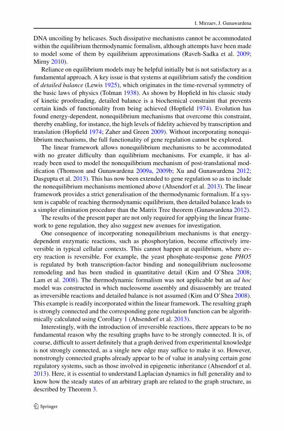
I. Mirzaev, J. Gunawardena
DNA uncoiling by helicases. Such dissipative mechanisms cannot be accommodatedwithin the equilibrium thermodynamic formalism, although attempts have been madeto model some of them by equilibrium approximations (Raveh-Sadka et al. 2009;Mirny 2010).
Reliance on equilibrium models may be helpful initially but is not satisfactory as afundamental approach. A key issue is that systems at equilibrium satisfy the conditionof detailed balance (Lewis 1925), which originates in the time-reversal symmetry ofthe basic laws of physics (Tolman 1938). As shown by Hopfield in his classic studyof kinetic proofreading, detailed balance is a biochemical constraint that preventscertain kinds of functionality from being achieved (Hopfield 1974). Evolution hasfound energy-dependent, nonequilibrium mechanisms that overcome this constraint,thereby enabling, for instance, the high levels of fidelity achieved by transcription andtranslation (Hopfield 1974; Zaher and Green 2009). Without incorporating nonequi-librium mechanisms, the full functionality of gene regulation cannot be explored.
The linear framework allows nonequilibrium mechanisms to be accommodatedwith no greater difficulty than equilibrium mechanisms. For example, it has al-ready been used to model the nonequilibrium mechanism of post-translational mod-ification (Thomson and Gunawardena 2009a, 2009b; Xu and Gunawardena 2012;Dasgupta et al. 2013). This has now been extended to gene regulation so as to includethe nonequilibrium mechanisms mentioned above (Ahsendorf et al. 2013). The linearframework provides a strict generalisation of the thermodynamic formalism. If a sys-tem is capable of reaching thermodynamic equilibrium, then detailed balance leads toa simpler elimination procedure than the Matrix Tree theorem (Gunawardena 2012).
The results of the present paper are not only required for applying the linear frame-work to gene regulation, they also suggest new avenues for investigation.
One consequence of incorporating nonequilibrium mechanisms is that energy-dependent enzymatic reactions, such as phosphorylation, become effectively irre-versible in typical cellular contexts. This cannot happen at equilibrium, where ev-ery reaction is reversible. For example, the yeast phosphate-response gene PHO5is regulated by both transcription-factor binding and nonequilibrium nucleosomeremodeling and has been studied in quantitative detail (Kim and O’Shea 2008;Lam et al. 2008). The thermodynamic formalism was not applicable but an ad hocmodel was constructed in which nucleosome assembly and disassembly are treatedas irreversible reactions and detailed balance is not assumed (Kim and O’Shea 2008).This example is readily incorporated within the linear framework. The resulting graphis strongly connected and the corresponding gene regulation function can be algorith-mically calculated using Corollary 1 (Ahsendorf et al. 2013).
Interestingly, with the introduction of irreversible reactions, there appears to be nofundamental reason why the resulting graphs have to be strongly connected. It is, ofcourse, difficult to assert definitely that a graph derived from experimental knowledgeis not strongly connected, as a single new edge may suffice to make it so. However,nonstrongly connected graphs already appear to be of value in analysing certain generegulatory systems, such as those involved in epigenetic inheritance (Ahsendorf et al.2013). Here, it is essential to understand Laplacian dynamics in full generality and toknow how the steady states of an arbitrary graph are related to the graph structure, asdescribed by Theorem 3.
Laplacian Dynamics on General Graphs
We have shown in this paper that the steady-state behavior of nonstrongly con-nected graphs is qualitatively different from that of strongly-connected graphs. Itcan exhibit considerable plasticity. A surprising amalgam of two distinct regulatorymodes has been revealed in yeast (Tirosh and Barkai 2008; Cairns 2009), wheremany genes incorporate, to varying degrees, the features of two extreme examples(Cairns 2009). One extreme consists of constitutively expressed genes with “open”promoters, which tend to have nucleosome-free regions and lack TATA boxes, whilethe other extreme consists of inducible genes with “covered” promoters, which haveTATA boxes and dynamically-shifting nucleosomes. At present there is insufficientquantitative analysis of different genes to know whether this amalgam can give riseto flexible responses due to nonstrong connectivity of the underlying graphs, but itremains an intriguing possibility for subsequent investigation.
Gene regulation is a single-molecule process—there is only one gene present—and stochasticity must be taken into account at the outset. Theorem 4 shows that thiscan be done with complete rigour while retaining the familiar biochemical intuitionfor molecules in solution. It may prove helpful in future work to exploit Theorem 4to translate the machinery of Markov process theory, as used to calculate averagesand higher moments of probability distributions, into the combinatorial language ofgraphs and trees. Such translation between different fields often leads to new insightsand may provide new tools for analysing fluctuations in gene expression.
It is of considerable topical importance to develop new methods for analysinggene regulation. The ENCODE project has recently provided a wealth of new dataabout the processes at work on DNA, including non-equilibrium processes such ashistone PTMs (Stamatoyannopoulos 2012). The linear framework provides a startingpoint from which such data can be formally represented in mathematical structures—labeled, directed graphs—from which the regulatory behavior of an individual genecan be inferred, without relying on the constraining assumption of thermodynamicequilibrium. The results of the present paper provide the mathematical foundationfor such biological analysis.
Acknowledgements We thank Arthur Jaffe for historical remarks on citations (Bott and Mayberry 1954;Jaffe 1965), David Perkinson for information about the proof in the Appendix, and an anonymous reviewerfor helpful comments. The work undertaken here was supported by the United States NSF under Grant0856285.
Appendix
We include for completeness a proof of the Matrix-Tree theorem as stated in Theo-rem 1. There are many versions of this and the one given here is adapted from DavidPerkinson’s handout,1 which is itself adapted from the proof in Tutte’s book (Tutte2001). This has the merits of being elementary, concise, and transparent. Let G be agraph on the vertices 1, . . . , n and let the symbols eij denote the labels on the edges:j → i, if, and only, if eij �= 0. The entries of L(G) are then given by Eq. (2).
1http://people.reed.edu/~davidp/412/handouts/matrix-tree.pdf.
I. Mirzaev, J. Gunawardena
The proof of Theorem 1 is in two steps, first for the special case of a principalminor, which is the essential part of the argument. Some additional notation willbe helpful. If A is any (not necessarily square) matrix let A[u,v] denote the matrixobtained from A by removing row u and column v. It is easier to work with thenegative Laplacian, L = −L(G), to keep control of the signs. Since the minor is thedeterminant of a (n − 1) × (n − 1) matrix, this change incurs a sign of (−1)n−1, sowe can rewrite Eq. (16) for the j th principal minor as
detL[j,j ] =∑
T ∈Θj (G)
( ∏k→l∈T
elk
), (42)
which is what we want to prove.
Proof The argument does not depend on j , so take j = 1 to simplify the notation.The determinant can be written in the standard form as
detL[1,1] =∑
π∈Sn−1
sign(π)Lπ(2)2 · · ·Lπ(n)n, (43)
where π : {2, . . . , n} → {2, . . . , n} is a permutation on {2, . . . , n}, Sn−1 is the symmet-ric group of all such permutations and sign(π) = ±1 is the sign of the permutation.A permutation can be uniquely expressed as a product of disjoint cycles, where thecycle (i1i2 · · · ik), with k > 1, is the permutation that sends iv to iv+1 for v < k andcycles around to send ik to i1. A permutation may also fix an element by sending j
to j and this is denoted by a degenerate cycle, (j). For example,
i 2 3 4 5 6 7π(i) 4 5 7 3 6 2
, π = (247)(35)(6).
A nonzero summand in Eq. (43), corresponding to the permutation π , can be writ-ten in terms of nonzero symbols eij �= 0 as follows. As mentioned above, π is aproduct of disjoint cycles. Each cycle gives rise to a product of nonzero symbols,
(i1i2 · · · ik) gives (−1)kei2i1ei3i2 · · · eikik−1ei1ik , (44)
where the signs arise because L is the negative of the Laplacian matrix defined byEq. (2). Each fixed point of π , π(j) = j , introduces into the overall product the sumof all the nondiagonal symbols in column j of L,∑
v �=j
evj , (45)
of which at least one symbol evj must be nonzero in order for the summand itself tobe nonzero. Each cycle of odd length contributes a sign of −1 through Eq. (44), whileeach cycle of even length contributes a sign of −1 to sign(π). The resulting overallproduct, when expanded out, is therefore a sum of monomials of the form
(−1)t ek22ek33 · · · eknn, (46)
where each symbol is nonzero, eki i �= 0, and t is the number of cycles in π .
Laplacian Dynamics on General Graphs
Monomials of the form in Eq. (46) have a natural interpretation in terms of thegraph G. They correspond to subgraphs of G in which there is exactly one outgo-ing edge from the vertices 2, . . . , n and no outgoing edge from vertex 1. Lets callthese special subgraphs. Given a special subgraph γ , it has an associated monomialeγ which is the product of the symbols on all the edges and it is evident that thiscorrespondence defines a bijection between special subgraphs and the monomials inEq. (46).
Special subgraphs have a distinctive structure: If we start at any vertex other than 1,then there is a unique path leading away from this vertex. Because G has only finitelymany vertices, this path must either intersect itself to form a cycle of edges or reachvertex 1 and stop. It follows that each connected component of a special subgrapheither contains an unique cycle or is a tree rooted at 1. (Recall that the connectedcomponents of a directed graph are the disjoint pieces into which the graph falls ifedge directions are ignored.) Of course, the cycle components may also contain tree-like spurs that lead to its unique cycle. Equation (44) shows that each cycle of edgesin G may be uniquely identified with a permutation cycle.
Suppose given a permutation π ∈ Sn−1 and a special subgraph γ . If all the cyclesof π appear as the cycles of cycle components of γ , then the symbols of any otheredges in γ , including those of any other cycle components of γ , can be constructedin π by using the elements fixed by π , since these introduce, through the terms inEq. (45), all the symbols needed for these remaining edges. It follows that eγ is oneof the monomials that appear when π is expanded into a sum of monomials throughEq. (46). Conversely, if eγ appears in the monomial expansion of π then the cyclesof π must occur among the cycles of cycle components of γ .
Given a special subgraph γ , we can now determine the multiplicity of eγ in thedeterminant in Eq. (43). Suppose that γ has s cycle components, where s > 0. Anypermutation π ∈ Sn−1 which uses exactly t of these cycles gives rise to eγ withmultiplicity (−1)t according to Eq. (46). There are
(st
)ways of choosing t cycle
components out of s. Considering all possibilities for t from t = 0 to t = s, the totalmultiplicity of eγ is
s∑t=0
(s
t
)(−1)t = (1 − 1)s = 0. (47)
This amazing cancellation is the heart of the Matrix-Tree theorem.The only remaining possibility is that γ has no cycle components, so that s = 0.
But then γ is a spanning tree rooted at 1. Moreover, eγ only appears as a monomialin the expansion of the identity permutation, whose monomial expansion is given by
n∏j=2
(∑v �=j
evj
). (48)
Evidently, eγ appears in Eq. (48) with multiplicity 1. Of course, Eq. (48) gives riseto monomials other than those coming from spanning trees rooted at 1 but theseother monomials disappear through cancellation because of Eq. (47). We are left withexactly the sum of monomials over rooted spanning trees in Eq. (42). �
I. Mirzaev, J. Gunawardena
To complete the proof of Theorem 1, it remains to deal with a non-principal mi-nor, detL[i,j ], which contributes the sign (−1)i+j to Eq. (16). This has nothing to dowith Laplacian matrices and depends only on the fact that 1 ·L(G) = 0. Some furthernotation will be helpful. Let A be a n× (n− 1) matrix and let Ai∗ denote its i-th row.We want to consider various (n − 1) × (n − 1) matrices made from these rows andwe will write these matrices by listing their rows in order. For instance, the (n− 1)×(n−1) submatrix of A in which the first row is omitted, is written [A2∗|A3∗| · · · |An∗].We will also use the convention that, in an ordered sequence, a bar over a term signi-fies its absence, so we can also write this same submatrix as [A1∗|A2∗| · · · |An∗].
Lemma 4 If A is any n × (n − 1) matrix for which 1 · A = 0, then
det[A1∗|A2∗| · · · |An∗
] = (−1)i−1 det[A1∗|A2∗| · · · |Ai∗| · · · |An∗
].
Proof Let B = [A1∗ +Ai∗|A2∗| · · · |Ai∗| · · · |An∗]. By construction, 1 ·B = 0, so thatdetB = 0. Because the determinant is multilinear,
det[A1∗|A2∗| · · · |Ai∗| · · · |An∗
] = (−1)det[Ai∗|A2∗| · · · |Ai∗| · · · |An∗
].
The determinant is also antisymmetric for interchange of rows, so that
det[Ai∗|A2∗| · · · |Ai∗| · · · |An∗
] = (−1)det[A2∗|Ai∗| · · · |Ai∗| · · · |An∗
].
It takes i − 2 successive row interchanges to bring Ai∗ back to where it originallywas in the list, from which the result follows. �
Now let A be the n × (n − 1) matrix obtained from L = −L(G) by removing thej th column. Then, using Lemma 4 twice, we see that
detL[i,j ] = det[A1∗| · · · |Ai∗| · · · |An∗
]= (−1)i−1 det
[A1∗| · · · |Ai∗| · · · |An∗
]= (−1)i+j−2 det
[A1∗| · · · |Aj∗| · · · |An∗
]= (−1)i+j detL[j,j ].
Combining this with Eq. (42) yields Eq. (16) and proves Theorem 1.
References
Ackers, G. K., Johnson, A. D., & Shea, M. A. (1982). Quantitative model for gene regulation by lambdaphage repressor. Proc. Natl. Acad. Sci. USA, 79, 1129–1133.
Agaev, R. P., & Chebotarev, P. Y. (2000). The matrix of maximum out forests of a digraph and its applica-tions. Autom. Remote Control, 61, 1424–1450.
Ahsendorf, T., Wong, F., Eils, R., & Gunawardena, J. (2013, in preparation). A framework for modellingeukaryotic gene regulation that accommodates non-equilibrium mechanisms.
Bintu, L., Buchler, N. E., Garcia, G. G., Gerland, U., Hwa, T., Kondev, J., Kuhlman, T., & Phillips, R.(2005a). Transcriptional regulation by the numbers: applications. Curr. Opin. Genet. Dev., 15, 125–135.
Laplacian Dynamics on General Graphs
Bintu, L., Buchler, N. E., Garcia, G. G., Gerland, U., Hwa, T., Kondev, J., & Phillips, R. (2005b). Tran-scriptional regulation by the numbers: models. Curr. Opin. Genet. Dev., 15, 116–124.
Bott, R., & Mayberry, J. P. (1954). Matrices and trees. In O. Morgenstern (Ed.), Economic activity analysis(pp. 391–400). New York: Wiley
Cairns, B. R. (2009). The logic of chromatin architecture and remodelling at promoters. Nature, 461, 193–198.
Chebotarev, P. (2010). Comment on ‘Consensus and cooperation in networked multi-agent systems’. Proc.IEEE, 98, 1353–1354.
Chebotarev, P., & Agaev, R. (2002). Forest matrices around the Laplacian matrix. Linear Algebra Appl.,356, 253–274.
Chebotarev, P. Y., & Agaev, R. P. (2009). Coordination in multiagent systems and Laplacian spectra ofdigraphs. Autom. Remote Control, 70, 469–483.
Chen, W. K. (1971). Applied graph theory. In Applied mathematics and mechanics, Amsterdam: North-Holland.
Chung, F. R. K. (1997). Spectral graph theory. Regional conference series in mathematics: Vol. 92. Provi-dence: Am. Math. Soc.
Colquhoun, D. (2006). The quantitative analysis of drug-receptor interactions: a short history. Trends Phar-macol. Sci., 27, 149–157.
Cornish-Bowden, A. (1995). Fundamentals of enzyme kinetics (2nd ed.). London: Portland Press.Dasgupta, T., Croll, D. H., Owen, J. A., Vander Heiden, M. G., Locasale, J. W., Alon, U., Cantley, L. C.,
& Gunawardena, J. (2013). A fundamental trade off in covalent switching and its circumvention inglucose homeostasis. Submitted.
Feinberg, M., & Horn, F. (1977). Chemical mechanism structure and the coincidence of the stoichiometricand kinetic subspace. Arch. Ration. Mech. Anal., 66, 83–97.
Gertz, J., Siggia, E. D., & Cohen, B. A. (2009). Analysis of combinatorial cis-regulation in synthetic andgenomic promoters. Nature, 457, 215–218.
Gunawardena, J. (2012). A linear framework for time-scale separation in nonlinear biochemical systems.PLoS ONE, 7, e36321.
He, X., Samee, M. A. H., Blatti, C., & Sinha, S. (2010). Thermodynamics-based models of transcriptionalregulation by enhancers: the roles of synergistic activation, cooperative binding and short-range re-pression. PLoS Comput. Biol., 6, e1000935.
Hill, T. L. (1966). Studies in irreversible thermodynamics IV. Diagrammatic representation of steady statefluxes for unimolecular systems. J. Theor. Biol., 10, 442–459.
Hill, T. L. (1985). Cooperativity theory in biochemistry: steady-state and equilibrium systems. Springerseries in molecular biology. New York: Springer.
Hirsch, M. W., & Smale, S. (1974). Differential equations, dynamical systems and linear algebra. Pureand applied mathematics. San Diego: Academic Press.
Hopfield, J. J. (1974). Kinetic proofreading: a new mechanism for reducing errors in biosynthetic processesrequiring high specificity. Proc. Natl. Acad. Sci. USA, 71, 4135–4139.
Horn, R. A., & Johnson, C. A. (1985). Matrix analysis. Cambridge: Cambridge University Press.Jaffe, A. (1965). Divergence of perturbation theory for bosons. Commun. Math. Phys., 1, 127–149.Janssens, H., Hou, S., Jaeger, J., Kim, A. R., Myasnikova, E., Sharp, D., & Reinitz, J. (2006). Quantitative
and predictive model of transcriptional control of the drosophila melanogaster even skipped gene.Nat. Genet., 38, 1159–1165.
van Kampen, N. G. (1992). Stochastic processes in physics and chemistry. Amsterdam: Elsevier.Kelly, F. P. (2011). Reversibility and stochastic networks. Cambridge: Cambridge University Press.Kenakin, T. (2005). New concepts in drug discovery: collateral efficacy and permissive antagonism. Nat.
Rev. Drug Discov., 4, 919–927.Kim, H. D., & O’Shea, E. K. (2008). A quantitative model of transcription factor-activated gene expression.
Nat. Struct. Mol. Biol., 15, 1192–1198.King, E. L., & Altman, C. (1956). A schematic method of deriving the rate laws for enzyme-catalyzed
reactions. J. Phys. Chem., 60, 1375–1378.Kirchhoff, G. (1847). Über die Auflösung der Gleichungen, auf welche man bei der Untersuchung der
linearen Verteilung galvanischer Ströme geführt wird. Ann. Phys. Chem., 72, 497–508.Koshland, D. E., Némethy, G., & Filmer, D. (1966). Comparison of experimental binding data and theo-
retical models in proteins containing subunits. Biochemistry, 5, 365–385.Kuhlman, T., Zhang, Z., Saier, M. H. Jr., & Hwa, T. (2007). Combinatorial transcriptional control of the
lactose operon of Escherichia coli. Proc. Natl. Acad. Sci. USA, 104, 6043–6048.
I. Mirzaev, J. Gunawardena
Lam, F. H., Steger, D. J., & O’Shea, E. K. (2008). Chromatin decouples promoter threshold from dynamicrange. Nature, 453, 246–250.
Lean, A. D., Stadel, J. M., & Lefkowitz, R. J. (1980). A ternary complex model explains the agonist-specific binding properties of the adenylate cyclase-coupled β-adrenergic receptor. J. Biol. Chem.,255, 7108–7117.
Lewis, G. N. (1925). A new principle of equilibrium. Proc. Natl. Acad. Sci. USA, 11, 179–183.Magnus, J. R., & Neudecker, H. (1988). Matrix differential calculus with applications in statistics and
econometrics. Chichester: WileyMerris, R. (1994). Laplacian matrices of graphs: a survey. Linear Algebra Appl., 198, 143–176.Michaelis, L., & Menten, M. (1913). Die kinetik der Invertinwirkung. Biochem. Z., 49, 333–369.Mirny, L. (2010). Nucleosome-mediated cooperativity between transcription factors. Proc. Natl. Acad. Sci.
USA, 107(22), 534–539.Monod, J., Wyman, J., & Changeux, J. P. (1965). On the nature of allosteric transitions: a plausible model.
J. Mol. Biol., 12, 88–118.Moon, J. W. (1970). Counting Labelled Trees. Canadian mathematical monographs: Vol. 1. Ottawa: Cana-
dian Mathematical Society.Nishikawa, T., & Motter, A. E. (2010). Network synchronization landscape reveals compensatory struc-
tures, quantization, and the positive effect of negative interactions. Proc. Natl. Acad. Sci. USA,107(10), 342–347.
Olfati-Saber, R., Fax, J. A., & Murray, R. M. (2007). Consensus and cooperation in networked multi-agentsystems. Proc. IEEE, 95, 215–233.
Olfati-Saber, R., & Murray, R. M. (2004). Consensus problems in networks of agents with switchingtopology and time-delays. IEEE Trans. Autom. Control, 49, 1520–1533.
Pecora, L. M., & Carroll, T. L. (1998). Master stability functions for synchronized coupled systems. Phys.Rev. Lett., 80, 2109–2112.
Raveh-Sadka, T., Levo, M., & Segal, E. (2009). Incorporating nucleosomes into thermodynamic modelsof transcription regulation. Genome Res., 19, 1480–1496.
Schnakenberg, J. (1976). Network theory of microscopic and macroscopic behaviour of master equationsystems. Rev. Mod. Phys., 48, 571–586.
Segal, E., Raveh-Sadka, T., Schroeder, M., Unnerstall, U., & Gaul, U. (2008). Predicting expression pattersfrom regulatory sequence in Drosophila segmentation. Nature, 451, 535–540.
Segal, E., & Widom, J. (2009). From DNA sequence to transcriptional behaviour: a quantitative approach.Nat. Rev. Genet., 10, 443–456.
Setty, Y., Mayo, A. E., Surette, M. G., & Alon, U. (2003). Detailed map of a cis-regulatory input function.Proc. Natl. Acad. Sci. USA, 100, 7702–7707.
Sherman, M. S., & Cohen, B. A. (2012). Thermodynamic state ensemble models of cis-regulation. PLoSComput. Biol., 8, e1002407.
Stamatoyannopoulos, J. (2012). What does our genome encode? Genome Res., 22, 1602–1611.Thomson, M., & Gunawardena, J. (2009a). The rational parameterisation theorem for multisite post-
translational modification systems. J. Theor. Biol., 261, 626–636.Thomson, M., & Gunawardena, J. (2009b). Unlimited multistability in multisite phosphorylation systems.
Nature, 460, 274–277.Tirosh, I., & Barkai, N. (2008). Two strategies for gene regulation by promoter nucleosomes. Genome
Res., 18, 1084–1091.Tolman, R. C. (1938). The principles of statistical mechanics. Oxford: Clarendon Press.Tutte, W. T. (1948). The dissection of equilateral triangles into equilateral triangles. Proc. Camb. Philol.
Soc., 44, 463–482.Tutte, W. T. (2001). Graph theory. Encyclopedia of mathematics and its applications: Vol. 21. Cambridge:
Cambridge University Press.Whitin, T. M. (1954). An economic application of ‘Matrices and trees’. In O. Morgenstern (Ed.), Economic
activity analysis (pp. 401–418). New York: WileyXu, Y., & Gunawardena, J. (2012). Realistic enzymology for post-translational modification: zero-order
ultrasensitivity revisited. J. Theor. Biol., 311, 139–152.Zaher, H. S., & Green, R. (2009). Fidelity at the molecular level: lessons from protein synthesis. Cell, 136,
746–762.Zinzen, R. P., Senger, K., Levine, M., & Papatsenko, D. (2006). Computational models for neurogenic
gene expression in the Drosophila embryo. Curr. Biol., 16, 1358–1365.


![On further ordering bicyclic graphs with respect to the ... · out that the Laplacian spectra radii of all these graphs are in the interval (n − 1;n]. In [16], Li et al. first](https://static.fdocuments.us/doc/165x107/5f0d0d097e708231d4386f53/on-further-ordering-bicyclic-graphs-with-respect-to-the-out-that-the-laplacian.jpg)