Lane Level Localization with Camera and Inertial ...

Lane Level Localization with Camera and Inertial Measurement Unit using anExtended Kalman Filter

by

Christopher Rose

A thesis submitted to the Graduate Faculty ofAuburn University

in partial fulfillment of therequirements for the Degree of

Master of Science

Auburn, AlabamaDecember 13, 2010

Keywords: Lane Departure Warning, Kalman Filter, Image Processing

Copyright 2010 by Christopher Rose

Approved by:

Thomas S. Denney, Chair, Professor of Electrical EngineeringDavid M. Bevly, Co-Chair, Associate Professor of Mechanical Engineering

Stanley Reeves, Professor of Electrical EngineeringCharles Stroud, Professor of Electrical Engineering

Abstract

This thesis studies a technique for combining vision and inertial measurement unit

(IMU) data to increase the reliability of lane departure warning systems. In this technique,

2nd-order polynomials are used to model the likelihood area of the location of the lane

marking position in the image as well as the lane itself. An IMU is used to predict the

drift of these polynomials and the estimated lane marking when the lane markings can not

be detected in the image. Subsequent frames where the lane marking is present results in

faster convergence of the model on the lane marking due to a reduced number of detected

erroneous lines.

A technique to reduce the effect of untracked lane markings has been employed which

bounds the previously detected 2nd-order polynomial with two other polynomials within

which lies the likelihood region of the next frame’s lane marking. Similarly, the slope at each

point on the lane marking model lies within a certain range with respect to the previously

detected 2nd-order polynomial. These bounds and slope employ similar characteristics as the

original line; therefore, the lane marking should be detected within the bounded area and

within the expected slope range given smooth transitions between each frame.

An inertial measurement unit can provide accelerations and rotation rates of a vehicle.

Using an extended Kalman filter, information from the IMU can be blended with the last

known coefficients of the estimated lane marking to approximate the lane marking coefficients

until the lane is detected. A measurement of the position within the lane can be carried out

by determining the number of pixels from the center of the image and the estimated lane

marking. This measurement value can then be converted to its real-world equivalent and

used to estimate the position of the vehicle within the lane. Also, the heading of the vehicle

ii

can be determined by examining the distance from the vanishing point of the camera and

the vanishing point of the lane markings.

iii

Acknowledgments

I would like to acknowledge the Federal Highway Administration for funding the project

that most of the work contained in this thesis is based upon. I would like to thank my parents

for their support. I would also like to thank all of the members of the GAVLAB for their

help. Specifically, I would like to thank John Allen and Jordan Britt - both of whom worked

with me on the Federal Highway project. Finally, I would like to thank Dr. David Bevly for

his advisement.

iv

Table of Contents

Abstract . . . . . . . . . . . . . . . . . . . . . . . . . . . . . . . . . . . . . . . . . . . ii

Acknowledgments . . . . . . . . . . . . . . . . . . . . . . . . . . . . . . . . . . . . . . iv

List of Figures . . . . . . . . . . . . . . . . . . . . . . . . . . . . . . . . . . . . . . . viii

1 Introduction . . . . . . . . . . . . . . . . . . . . . . . . . . . . . . . . . . . . . . 1

1.1 Vehicle Safety . . . . . . . . . . . . . . . . . . . . . . . . . . . . . . . . . . . 1

1.2 Limitations of GPS . . . . . . . . . . . . . . . . . . . . . . . . . . . . . . . . 2

1.3 Cameras . . . . . . . . . . . . . . . . . . . . . . . . . . . . . . . . . . . . . . 2

1.3.1 Image Acquisition . . . . . . . . . . . . . . . . . . . . . . . . . . . . . 2

1.3.2 Lane Detection using Vision . . . . . . . . . . . . . . . . . . . . . . . 4

1.4 Camera/IMU Solution . . . . . . . . . . . . . . . . . . . . . . . . . . . . . . 5

1.5 Thesis Contributions . . . . . . . . . . . . . . . . . . . . . . . . . . . . . . . 6

2 Background . . . . . . . . . . . . . . . . . . . . . . . . . . . . . . . . . . . . . . 8

2.1 Navigation Sensors . . . . . . . . . . . . . . . . . . . . . . . . . . . . . . . . 8

2.1.1 GPS . . . . . . . . . . . . . . . . . . . . . . . . . . . . . . . . . . . . 8

2.1.2 Inertial Measurement Unit . . . . . . . . . . . . . . . . . . . . . . . . 10

2.1.3 GPS/INS System . . . . . . . . . . . . . . . . . . . . . . . . . . . . . 12

2.1.4 Vision Systems . . . . . . . . . . . . . . . . . . . . . . . . . . . . . . 12

2.2 Lane Level Localization . . . . . . . . . . . . . . . . . . . . . . . . . . . . . 23

2.2.1 Kalman Filter . . . . . . . . . . . . . . . . . . . . . . . . . . . . . . . 23

2.2.2 Differential GPS . . . . . . . . . . . . . . . . . . . . . . . . . . . . . 24

2.2.3 Inertial / Vision Sensor Fusion . . . . . . . . . . . . . . . . . . . . . . 25

2.3 Conclusions . . . . . . . . . . . . . . . . . . . . . . . . . . . . . . . . . . . . 26

3 Vision System . . . . . . . . . . . . . . . . . . . . . . . . . . . . . . . . . . . . . 27

v

3.1 Lane Marking Line Selection . . . . . . . . . . . . . . . . . . . . . . . . . . . 29

3.1.1 Thresholding . . . . . . . . . . . . . . . . . . . . . . . . . . . . . . . 29

3.1.2 Edge Detection . . . . . . . . . . . . . . . . . . . . . . . . . . . . . . 35

3.1.3 Line Extraction and Selection . . . . . . . . . . . . . . . . . . . . . . 36

3.2 Least Squares Polynomial Interpolation . . . . . . . . . . . . . . . . . . . . . 38

3.3 Polynomial Boundary Curves . . . . . . . . . . . . . . . . . . . . . . . . . . 41

3.4 Lateral Displacement Measurement . . . . . . . . . . . . . . . . . . . . . . . 42

3.5 Heading Measurement . . . . . . . . . . . . . . . . . . . . . . . . . . . . . . 43

3.6 Linear Kalman Filter . . . . . . . . . . . . . . . . . . . . . . . . . . . . . . . 47

3.7 Performance in Different Environments . . . . . . . . . . . . . . . . . . . . . 49

3.7.1 Performance under Varying Lighting Conditions . . . . . . . . . . . . 49

3.7.2 Performance in a City . . . . . . . . . . . . . . . . . . . . . . . . . . 51

3.7.3 Performance in Heavy Precipitation . . . . . . . . . . . . . . . . . . . 52

3.8 Experimental Results - Vision System . . . . . . . . . . . . . . . . . . . . . . 54

3.8.1 Polynomial Coefficient State Estimation . . . . . . . . . . . . . . . . 54

3.8.2 Calculated Lateral Distance and True Lateral Distance . . . . . . . . 55

3.8.3 Calculated Heading and True Heading . . . . . . . . . . . . . . . . . 56

3.9 Conclusions . . . . . . . . . . . . . . . . . . . . . . . . . . . . . . . . . . . . 57

4 Vision/Inertial System . . . . . . . . . . . . . . . . . . . . . . . . . . . . . . . . 60

4.1 System Overview . . . . . . . . . . . . . . . . . . . . . . . . . . . . . . . . . 60

4.2 Extended Kalman Filter . . . . . . . . . . . . . . . . . . . . . . . . . . . . . 61

4.2.1 Road Frame . . . . . . . . . . . . . . . . . . . . . . . . . . . . . . . . 61

4.2.2 Filter Structure . . . . . . . . . . . . . . . . . . . . . . . . . . . . . . 62

4.3 Time Update . . . . . . . . . . . . . . . . . . . . . . . . . . . . . . . . . . . 63

4.3.1 Continuous Update . . . . . . . . . . . . . . . . . . . . . . . . . . . . 63

4.3.2 Vision System Time Update . . . . . . . . . . . . . . . . . . . . . . . 66

4.4 Measurement Update . . . . . . . . . . . . . . . . . . . . . . . . . . . . . . . 72

vi

4.5 Observability Analysis . . . . . . . . . . . . . . . . . . . . . . . . . . . . . . 73

4.6 Vision/IMU Experimental Results . . . . . . . . . . . . . . . . . . . . . . . . 75

4.6.1 Inputs and Bias Estimates . . . . . . . . . . . . . . . . . . . . . . . . 77

4.6.2 Impact of Measurements on State Estimates . . . . . . . . . . . . . . 79

4.6.3 Comparison with Truth . . . . . . . . . . . . . . . . . . . . . . . . . 81

4.7 Conclusions . . . . . . . . . . . . . . . . . . . . . . . . . . . . . . . . . . . . 85

5 Summary and Conclusions . . . . . . . . . . . . . . . . . . . . . . . . . . . . . . 88

5.1 Future Work . . . . . . . . . . . . . . . . . . . . . . . . . . . . . . . . . . . . 89

Bibliography . . . . . . . . . . . . . . . . . . . . . . . . . . . . . . . . . . . . . . . . 91

Appendices . . . . . . . . . . . . . . . . . . . . . . . . . . . . . . . . . . . . . . . . . 94

A Truth Data . . . . . . . . . . . . . . . . . . . . . . . . . . . . . . . . . . . . . . 95

A.1 Obtaining Truth Data . . . . . . . . . . . . . . . . . . . . . . . . . . . . . . 95

B Implementation . . . . . . . . . . . . . . . . . . . . . . . . . . . . . . . . . . . . 100

B.1 Vision System . . . . . . . . . . . . . . . . . . . . . . . . . . . . . . . . . . . 100

B.2 Vision/IMU Fusion . . . . . . . . . . . . . . . . . . . . . . . . . . . . . . . . 105

C Alternate EKF Structure . . . . . . . . . . . . . . . . . . . . . . . . . . . . . . . 107

C.1 Closely-Coupled EKF . . . . . . . . . . . . . . . . . . . . . . . . . . . . . . . 107

C.2 Lateral Acceleration . . . . . . . . . . . . . . . . . . . . . . . . . . . . . . . 108

vii

List of Figures

2.1 Intersecting Spheres . . . . . . . . . . . . . . . . . . . . . . . . . . . . . . . . 9

2.2 Pinhole Camera Model . . . . . . . . . . . . . . . . . . . . . . . . . . . . . . 12

2.3 Sample Image and Histogram . . . . . . . . . . . . . . . . . . . . . . . . . . 16

2.4 Example Initial Image . . . . . . . . . . . . . . . . . . . . . . . . . . . . . . 21

2.5 Hough Transform of Initial Image . . . . . . . . . . . . . . . . . . . . . . . . 22

3.1 Overview of System . . . . . . . . . . . . . . . . . . . . . . . . . . . . . . . . 27

3.2 Highway Image and Thresholded Image . . . . . . . . . . . . . . . . . . . . . 29

3.3 Intensity Image Histogram . . . . . . . . . . . . . . . . . . . . . . . . . . . . 30


3.5 Intensity Image for Darker Image . . . . . . . . . . . . . . . . . . . . . . . . 32

3.6 Image Channels . . . . . . . . . . . . . . . . . . . . . . . . . . . . . . . . . . 33

3.7 Highway Image and Averaged Inverted Saturation and Value Image . . . . . 33

3.8 Average Image Histogram . . . . . . . . . . . . . . . . . . . . . . . . . . . . 34


3.10 Darker Highway Image and Dynamically Thresholded Image . . . . . . . . . 35

3.11 Darker Highway Image and Dynamically Thresholded Image . . . . . . . . . 35

3.12 Various methods of edge detection . . . . . . . . . . . . . . . . . . . . . . . . 36

3.13 Hough Lines . . . . . . . . . . . . . . . . . . . . . . . . . . . . . . . . . . . . 37

3.14 Polynomial Boundary Curves . . . . . . . . . . . . . . . . . . . . . . . . . . 39

3.15 Lane Marking Interpolation . . . . . . . . . . . . . . . . . . . . . . . . . . . 40

viii

3.16 Polynomial Bounding Lines . . . . . . . . . . . . . . . . . . . . . . . . . . . 42

3.17 Determining distance . . . . . . . . . . . . . . . . . . . . . . . . . . . . . . . 43

3.18 Determining Heading . . . . . . . . . . . . . . . . . . . . . . . . . . . . . . . 45

3.19 Bird’s Eye View of Road for Determining Heading . . . . . . . . . . . . . . . 46

3.20 Night Scene and Edge Map . . . . . . . . . . . . . . . . . . . . . . . . . . . 50

3.21 Night Scene at the Track and Edge Map . . . . . . . . . . . . . . . . . . . . 50

3.22 Flash of light from sun peering through treetops during twilight . . . . . . . 51

3.23 City Street and Edge Map . . . . . . . . . . . . . . . . . . . . . . . . . . . . 51

3.24 City Stoplight Image and Edge Map . . . . . . . . . . . . . . . . . . . . . . 52

3.25 Shadows Created by Buildings at Intersections . . . . . . . . . . . . . . . . . 52

3.26 Precipitation - Day and Night . . . . . . . . . . . . . . . . . . . . . . . . . . 53

3.27 Coefficient B Measurement (Blue) and Filtered Estimate (Red) . . . . . . . . 55

3.28 Coefficient C Measurement (Blue) and Filtered Estimate (Red) . . . . . . . . 56

3.29 True Lateral Distance and Calculated Lateral Distance for Vision System OnFull Track Test Run . . . . . . . . . . . . . . . . . . . . . . . . . . . . . . . 57

3.30 Lateral Distance Error for Vision System On Full Track Test Run . . . . . . 58

3.31 True Heading and Measured Heading for Vision System On Full Track TestRun . . . . . . . . . . . . . . . . . . . . . . . . . . . . . . . . . . . . . . . . 59

3.32 Heading Error for Vision System On Full Track Test Run . . . . . . . . . . . 59

4.1 Loosely Coupled Sensor Fusion . . . . . . . . . . . . . . . . . . . . . . . . . 61

4.2 Road and Body Frame . . . . . . . . . . . . . . . . . . . . . . . . . . . . . . 62

4.3 Kalman filter time update coefficient change for the linear lane model . . . . 71

4.4 Longitudinal Acceleration and Bias . . . . . . . . . . . . . . . . . . . . . . . 78

4.5 Yaw Rate and Bias . . . . . . . . . . . . . . . . . . . . . . . . . . . . . . . . 79

4.6 Longitudinal Velocity Estimate vs. Measurement . . . . . . . . . . . . . . . 81

4.7 Heading Estimate and Measurement . . . . . . . . . . . . . . . . . . . . . . 82

ix

4.8 Lateral Distance Estimate and Measurement . . . . . . . . . . . . . . . . . . 83

4.9 Lateral Distance Truth vs. Estimate . . . . . . . . . . . . . . . . . . . . . . 84

4.10 Dead Reckoning Lane Estimation . . . . . . . . . . . . . . . . . . . . . . . . 85

4.11 Lateral Distance Error . . . . . . . . . . . . . . . . . . . . . . . . . . . . . . 86

4.12 Heading Truth vs. Estimate . . . . . . . . . . . . . . . . . . . . . . . . . . . 87

4.13 Heading Error . . . . . . . . . . . . . . . . . . . . . . . . . . . . . . . . . . . 87

A.1 Cubic Spline Interpolation of Survey Points to Reduce Error . . . . . . . . . 96

A.2 Determination of True Heading and Lateral Distance from GPS position . . 99

B.1 Initial Image Processing . . . . . . . . . . . . . . . . . . . . . . . . . . . . . 100

B.2 Hough Line Selection . . . . . . . . . . . . . . . . . . . . . . . . . . . . . . . 102

B.3 Line Processing . . . . . . . . . . . . . . . . . . . . . . . . . . . . . . . . . . 103

B.4 IMU/Camera Integration . . . . . . . . . . . . . . . . . . . . . . . . . . . . . 106

C.1 Closely Coupled Lateral Distance Estimate vs. Truth . . . . . . . . . . . . . 108

C.2 Closely Coupled Heading Estimate vs. Truth . . . . . . . . . . . . . . . . . . 109

C.3 Lateral Acceleration . . . . . . . . . . . . . . . . . . . . . . . . . . . . . . . 110

x

Chapter 1

Introduction

1.1 Vehicle Safety

Motor vehicle crashes are the leading cause of death among Americans from 1 to 34

years of age. In 2008, 37,261 people died from accidents on the United States’ highways. Of

those deaths, 19,794 (53%) were due to road departure. Road departures are defined by the

Federal Highway Administration (FHWA) as a non-intersection crash which occurs after a

vehicle has crossed an edge line or a center line, or has left the traveled path. 24% of crashes

in 2008 were the result of running off the right side of the road, 10% due to running off

the left side of the road, and 17% due to crossovers. Certainly, fewer lane departures would

result in fewer crashes on the road [1].

One cause for road departure is driver distraction. 5,870 people were killed and 515,000

people were injured in 2008 due to distracted driving, according to crash report records.

Distracted driving consists of focusing attention on activities other than driving such as

cell phone use, texting, eating, drinking, conversing with passengers, and interacting with

in-vehicle technologies and portable electronic devices. The National Motor Vehicle Crash

Causation Survey (NMVCCS) was a nationwide survey on 5,471 crashes involving light

passenger vehicles with a focus on factors related to events before the crash occurred. Re-

searchers in this survey were allowed permission to be on the scene of the crash to assess

the critical event of the crash, such as running off the edge of the road, failure to stay in the

proper lane, or loss of control of the vehicle. For crashes where the driver was deemed re-

sponsible for the crash, 18% were reported to have involved driver distraction [2]. Avoidance

of these types of crashes would save many lives.

1

1.2 Limitations of GPS

The Global Positioning System (GPS) is often used today in applications for vehicle

navigation, consumer path-finding applications, military use, and surveying. Each of these

systems are limited in environments where line to sight exists to GPS satellites. However,

some areas such as heavily forested or urban streets (urban canyon) generally do not provide

line of sight to satellites. In these areas, GPS is not available and must normally be combined

with an inertial navigation system to provide information during these portions where GPS

is not available.

The accuracy of a typical GPS system is less than 10 meters [3]. For lane level positioning

(localization within a lane), this accuracy is insufficient for a typical lane width of 3.66 meters.

Error associated with integration error in a GPS/Inertial Navigation System (INS) system

can lead to large errors if GPS cannot reconfigure the Inertial Measurement Unit (IMU)

due to shadowed environments. Differential GPS, where known base stations broadcast

corrections to GPS signals, can provide accuracies into the centimeter range, but line of

sight to the base station and satellites is needed [3].

Even with differential GPS accuracy, position with respect to the world is not helpful

without knowledge of the position of the lane markings themselves. Maps with the position

of the lane markings can be used with differential GPS for lane level positioning as long as

any errors associated with the GPS drift from day to day are insignificant.

1.3 Cameras

1.3.1 Image Acquisition

A simple image formation model is based on the amount of source illumination on the

scene and the amount of illumination reflected by objects in the scene. If f(x, y) is the value

of a point in an image, then

2

f(x, y) = i(x, y)r(x, y) (1.1)

where i is the illumination from the source and r is the reflectance of an object in the image.

The minimum value of f and the maximum value of f create an interval known as the

grayscale. This interval is usually normalized in the range [0, 1] where 0 is black and 1 is

white. Any sensor which creates images usually produces a continuous voltage waveform

whose amplitude and spatial behavior are related to the phenomenon being sensed. These

sensors include computerized axial tomography (CAT) imaging, magnetic resonance imaging

(MRI), and typical digital cameras. Each sensor output must be sampled and quantized in

order to create a digital image. A typical digital camera has an array of sensors called charge-

coupled devices (CCD). The array produces outputs that are proportional to the integral of

the light received at each CCD. The light is focused using a lens to collect the information

from the scene [4].

Color in images is represented in many different models. One of the more well known

color models is the red-green-blue (RGB) color model, in which each color is represented

as a combination of red, green, and blue. This model is typically represented as a cube,

where each axis represents the strength of the red, green, and blue intensities. Color images

are obtained by using filters sensitive to red, green, and blue. When combined, these three

images form a color image. A more intuitive color model is the Hue, Saturation, Intensity

(HSI) color model which is similar to the way humans view color. The hue channel in this

color model contains the pure color information obtained from the image. The saturation

channel contains information on the amount of white light diluted into that pure color.

The intensity channel describes the intensity component of the image and can essentially be

considered a grayscale image. The geometric representation of the HSI color model can be

gleaned from the RGB color model by creating a cylindrical representation of the RGB model

where the vertical axis corresponds to intensity, the angle corresponds to hue, and the radial

distance from the origin corresponds to the amount of saturation. In this representation,

3

the circle corresponding to zero height (zero intensity) is fully black, and for this reason the

model is sometimes represented as an inverted cone, where the point of the cone corresponds

to black [4].

1.3.2 Lane Detection using Vision

Camera vision has already been implemented in lane departure warning (LDW) systems

in commercial vehicles. These systems detect when the vehicle has left or is about to leave

a lane and emit a warning for the driver. One such system, by Lee et al. [5], incorporates

perception-net to determine the lateral offset and time to lane crossing (TLC), which warns

the driver when a lane departure is or may soon take place. A fuzzy evolutionary algorithm

was used by Kim and Oh [6] to determine the lateral offset and TLC using a selected

hazard level for lane departure warning. Another LDW system, by Jung and Kelber [7],

used a linear-parabolic model to create a LDW system using lateral offset based on the near

field and far field. For the near field close to the camera’s position in a forward looking

camera, a linear function was used to capture the straight appearance of the road close

to the car. For the far field, a parabolic model was used to model the curves of the road

ahead. In their following paper [8], Jung and Kelber used their system with the linear-

parabolic model to compute the lateral offset without camera parameters. Hsiao and others

[9] avoided the use of the Hough transform and instead relied on peak and edge finding, edge

connection, line-segment combination, and lane boundary selection for their LDW system.

In [10], optical flow was used to achieve lane recognition under adverse weather conditions.

Feng [11] used an improved Hough transform to obtain the road edge in a binary image,

followed by establishment of an area of interest based on the prediction result of a Kalman

filter. In [12], an extended Kalman filter was used to model the lane markings to search

within a specified area in the image so that far lane boundaries are searched with a smaller

area than closer lane boundaries, thus reducing the impact of noise.

4

Three dimensional road modeling has become a popular method to reduce the errors

associated with lane detection in image space. The clothoid is an often used model for

three-dimensional reconstruction due to its linearly changing arc length. Dickmanns and

Mysliwetz [13] used the clothoid parameters to recognize horizontal and vertical road pa-

rameters in a recursive manner. Khosla [14] used two contiguous clothoid segments with

different geometries but with continuous curvature across each clothoid, which gives a closed

form parametric expression for the model. However, Swartz [15] argues that the clothoid

model for the road is unsuitable for sensor fusion due to the “sloshing” effect of the estimated

values between the clothoid parameters.

Knowledge of the lane geometry in front of the vehicle gives information to the driver or

autonomous navigation system, such as the distance within the lane, whether or not a turn is

located ahead, the road structure ahead for mapping, or map matching to identify the current

location of the vehicle. However, camera systems have limitations due to non-ideal visual

conditions. Additional road markings on the ground, such as that of a crosswalk, turn arrow,

or merged lane, can introduce rogue lines into the image and shift the estimated lines beyond

that of the actual lane marking. Phantom lines detected from the Hough transform that are

not readily apparent in the image itself can arise unexpectedly. Dashed lane markings of the

center road can reduce its detection rate and lead to gaps in the measurement data for that

lane marking.

1.4 Camera/IMU Solution

Often, environmental conditions prevent a clear view of the lane markings. The amount

of light, objects in the road, and even loss of the lane marking itself can lead to periods in

which the lane is no longer detectable. During these conditions, the camera systems cannot

give a good indication of the vehicle’s position within the lane. However, an IMU can provide

indications of the vehicle’s dynamics within the lane (assuming a straight road) similar to

5

its role in a GPS/INS setup. This thesis will outline how a camera and IMU system was

developed for lane positioning.

1.5 Thesis Contributions

This thesis studies a technique for combining vision and IMU data to increase the

reliability of lane departure warning systems. In this technique, 2nd-order polynomials are

used to model the likelihood area of the location of the lane marking position in the image

as well as the lane itself. An IMU is used to predict the drift of these polynomials and the

estimated lane marking when the lane markings can not be detected in the image. Subsequent

frames where the lane marking is present results in faster convergence of the model on the

lane marking due to a reduced number of detected erroneous lines.

A technique to reduce the effect of untracked lane markings has been employed which

bounds the previously detected 2nd-order polynomial with two other polynomials within

which lies the likelihood region of the next frame’s lane marking. These bounds employ

similar characteristics as the original line; therefore, the lane marking is detected within the

bounded area given smooth transitions between each frame.

An IMU can provide accelerations and rotation rates of a vehicle. Using an extended

Kalman filter, information from the IMU can be blended with the last known coefficients

of the estimated lane marking to approximate the lane marking coefficients until the lane is

detected. A measurement of the position within the lane can be carried out by determining

the number of pixels from the center of the image and the estimated lane marking. This

measurement value can then be converted to its real-world equivalent and used to estimate

the position of the vehicle within the lane.

Structure from motion and visual odometry both require large states for tracking land-

mark points from image to image. These landmark points are replaced with just six states

in the presented filter for the lane model (aL, bL, cL, aR, bR, cR). The use of this lane model

allows for consecutive frames with independent features — the tracked landmarks, such as

6

trees, grass, asphalt, etc., in typical structure from motion and visual odometry filters, do

not need to coexist from frame to frame as long as the lane markings are visible. As such,

most landmark trackers have upper limits in terms of speed of the camera (longitudinally or

laterally) with which the algorithm functions due to the need to track the individual land-

marks across consecutive frames. To increase this upper limit, the number of frames taken

per second from the camera would need to be increased.

Specific contributions of this thesis include the development of a system for lane tracking

using vision and fusion of that vision system with other sensors for lane tracking during

failures of the camera to detect the system. Within the image processing algorithm, a

selection process for valid lines of the image was developed using polynomial bounds and

slope selection. Lateral distance within the lane and heading were determined from the

camera image. An extended Kalman filter was used to fuse the image processing with

inertial measurements from an IMU and with longitudinal measurements from GPS. With

this filter, the lane markings were tracked in the image even in the absence of detection from

the image itself. This thesis includes an analysis of experimental results with real data and

will show that the sensor fusion improves the performance of the system for lane tracking

even in periods where lanes cannot be detected by the camera.

Chapter 1 introduced the problem of vehicle safety and lane localization. Chapter

2 describes the background of various components of the system that were not actively

researched in the development of this filter. Chapter 3 presents a sequential overview of the

image processing involved in detecting the lane markings, finding the heading and lateral

distance within the lane from the camera, and presents experimental results of the algorithm.

Chapter 4 shows the extension of the image processing by including the IMU inputs for

lane tracking when the camera does not detect the lane markings. It also includes the

experimental results for the lane tracking system with an analysis of the performance and

drawbacks of the system. Finally Chapter 5 summarizes the work presented and discusses

future work.

7

Chapter 2

Background

2.1 Navigation Sensors

Many navigation systems combine an IMU and GPS in order to determine the location

of a vehicle. The IMU provides high data rates at the cost of integration drift while GPS

provides more accurate measurements at slower rates. Similarly, cameras provide passive,

accurate measurements at lower rates. At low velocities, cameras can track very accurately,

but higher speeds create motion blur and limitations of camera sampling rates [16]. Inertial

sensors, however, have large measurement uncertainty at slow motion and lower relative

uncertainty at high velocities [16]. IMU’s and cameras, then, are complementary, and each

possesses its own respective strengths.

2.1.1 GPS

GPS provides positioning data across the world. Satellites in orbit around the earth

send ranging signals to receivers about their location. With enough satellites, a receiver is

able to determine its approximate location. The determination of a receiver’s location is

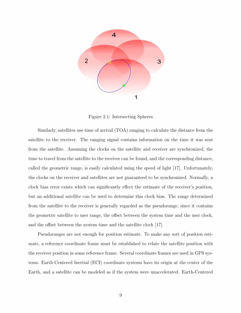
based on the concept of intersecting spheres, where each sphere represents the distance from

a satellite. Fig. 2.1 shows the concept of intersecting spheres. Two intersecting spheres,

spheres 1 and 2 in Fig. 2.1, create a circle, shown in blue. An additional sphere, sphere

3, creates two points, shown as yellow and green, located on the plane of intersection of

the original two spheres. Generally for land based applications, the correct point lies near

the surface of the earth, and the other point can be ignored. For aviation applications, an

additional satellite, sphere 4, may be needed to determine which of the two points is correct,

shown as the yellow point as the intersection of all of the spheres [17].

8

1

2 3

4

Figure 2.1: Intersecting Spheres

Similarly, satellites use time of arrival (TOA) ranging to calculate the distance from the

satellite to the receiver. The ranging signal contains information on the time it was sent

from the satellite. Assuming the clocks on the satellite and receiver are synchronized, the

time to travel from the satellite to the receiver can be found, and the corresponding distance,

called the geometric range, is easily calculated using the speed of light [17]. Unfortunately,

the clocks on the receiver and satellites are not guaranteed to be synchronized. Normally, a

clock bias error exists which can significantly effect the estimate of the receiver’s position,

but an additional satellite can be used to determine this clock bias. The range determined

from the satellite to the receiver is generally regarded as the pseudorange, since it contains

the geometric satellite to user range, the offset between the system time and the user clock,

and the offset between the system time and the satellite clock [17].

Pseudoranges are not enough for position estimate. To make any sort of position esti-

mate, a reference coordinate frame must be established to relate the satellite position with

the receiver position in some reference frame. Several coordinate frames are used in GPS sys-

tems. Earth-Centered Inertial (ECI) coordinate systems have its origin at the center of the

Earth, and a satellite can be modeled as if the system were unaccelerated. Earth-Centered

9

Earth-Fixed reference frame (ECEF) rotates with the earth in order to more easily compute

the latitude, longitude, and height parameters of most GPS receivers [17].

GPS has limitations, however. For positioning within a lane, the location of the lane

markings themselves must be known. Knowledge of location with respect to the world using

GPS means little for determining the location within a lane if the lane location is not known.

Also, a GPS signal will either be degraded or completely lost without line-of-sight to the

GPS satellites. In some environments such as urban canyons, the number of visible satellites

can fall below the required number of satellites (four), and a position cannot be estimated.

Many solutions for this problem have been proposed, such as the use of IMU’s to obtain a

solution when GPS is not available [17].

2.1.2 Inertial Measurement Unit

IMU’s typically have three orthogonal accelerometers and three orthogonal gyroscopes

to measure accelerations and rotation rates in three dimensions. The position and orientation

can be found by integrating these measurements.

Gyroscopes

Gyroscopes operate on the principle of the conservation of angular momentum. The

mechanical gyroscope is essentially a spinning wheel on an axle. Once spinning, the gyroscope

resists changes to its orientation. The net force on the gyroscope is due to all of the particles

in the spinning wheel which results in a moment due to Coriolis acceleration of

M = Iw × p (2.1)

where I is the moment of inertia of the spinning wheel, p is the angular velocity of the

spinning wheel, and w is the angular velocity of the gyroscope. As the orientation of the gy-

roscope changes, it creates an opposing moment which can be measured. This measurement

is proportional to the angular rate [16].

10

Since a spinning wheel on an axle is unreasonable for most real-world applications, the

principle of the mechanical gyroscope is applied in the vibrating structure gyroscope. This

gyroscope has no spinning disk and is based on producing radial linear motion and measuring

the Coriolis effect induced by rotation. A flexing beam is made to vibrate in a plane, and

rotation about the axis of that beam induces a Coriolis force that moves the beam sideways.

This movement can be measured and used to determine the rotation rate of the gyroscope.

Most real-world applications use these MEMS gyroscopes with a single piece of silicon [16].

One of the main factors in the quality of any inertial system is the drift of the gyroscopes.

This drift is caused by manufacturing deficiencies such as mass unbalances in the rotating

mass of the gyroscope and by nonlinearities in the pickoff circuits of fiber-optic gyroscopes.

As accuracy of the gyroscope improves, more expensive manufacturing techniques are needed,

and the cost of the IMU increases greatly [17].

Accelerometer

Accelerometers are based on the acceleration of a mass on an elastic element and measure

specific force. A viscous damper provides damping proportional to the relative velocity of

the proof mass and the sensor body. The dynamics of the system are described as

x(t) + 2ζωnx(t) + ω2nx(t) = −y(t) (2.2)

where y(t) is acceleration of the sensor body, x(t) is displacement, ωn is natural frequency,

and ζ is damping ratio. Three types of accelerometers are prevalent: capacitive, piezoelectric,

and piezo-resistive. Because piezoelectric sensors lack a DC response, they are unsuitable

for an inertial navigation system. In piezo-resistive accelerometers, a piezoresistor measures

the position of the proof mass. In a capacitive accelerometer, the proof mass position is

measured by measuring the change in capacitance [16].

11

2.1.3 GPS/INS System

GPS and IMU’s are complementary systems. GPS gives bounded accuracy but slow

update rates, while IMU’s provide high data rates at the cost of integration drift. In a

GPS/INS solution, the GPS is used to calibrate the IMU to counter the integration drift

and bound the error. When GPS is not available, the IMU can give an estimate of the

position using dead reckoning until GPS measurements are once again available. IMU data

can also be used to verify validity of GPS measurements. GPS pseudorange measurements

can be compared to the 6-sigma deviation limit to exclude anomalous satellite data [17].

2.1.4 Vision Systems

Camera models are used to describe the projection of a three-dimensional scene onto

a two-dimensional image. The pinhole camera model, shown in Fig. 2.2, considers a single

center of projection where all rays originating from each world point converge. The image,

then, is the projection of all points in the world to that point. The pinhole camera model

ignores lens distortion and assumes there is no skew. A world point P , represented in three

dimensions by (X, Y, Z), is projected onto the image, represented by (u, v), through point p

to the center of projection.

X

Y

Z

Center of projection

Virtual Image Plane

uv

Focal length

Optical axis

pP

Figure 2.2: Pinhole Camera Model

12

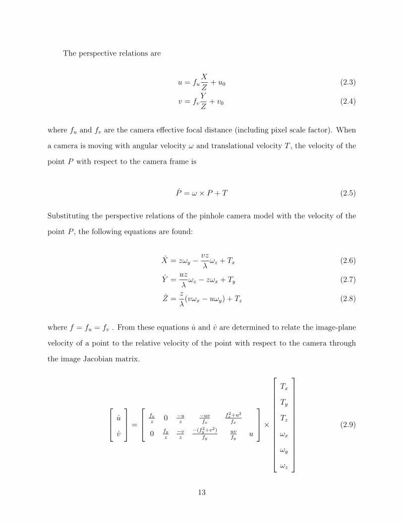
The perspective relations are

u = fuX

Z+ u0 (2.3)

v = fvY

Z+ v0 (2.4)

where fu and fv are the camera effective focal distance (including pixel scale factor). When

a camera is moving with angular velocity ω and translational velocity T , the velocity of the

point P with respect to the camera frame is

P = ω × P + T (2.5)

Substituting the perspective relations of the pinhole camera model with the velocity of the

point P , the following equations are found:

X = zωy −vz

λωz + Tx (2.6)

Y =uz

λωz − zωx + Ty (2.7)

Z =z

λ(vωx − uωy) + Tz (2.8)

where f = fu = fv . From these equations u and v are determined to relate the image-plane

velocity of a point to the relative velocity of the point with respect to the camera through

the image Jacobian matrix.

u

v

=

fxz

0 −uz

−uvfx

f2x+u2

fx

0 fyz

−vz

−(f2y+v2)fy

uvfy

u

×

Tx

Ty

Tz

ωx

ωy

ωz

(2.9)

13

Velocity in the image plane is the sum of six motion components, which makes it impossible

to distinguish rotational from translational motion with a single point. The translational

components of image-plane velocity have the range z which represents the effect of range on

apparent velocity — a slow, close object appears to move at the same speed as a distant fast

object [1].

Camera systems have already been developed which can detect lanes or predict lane

departures and warn the driver. These camera systems detect the location of the lane

markings and determine a possible time to lane crossing. If the approach to a lane marking

is too fast or the vehicle has crossed the lane marking, a warning will sound, which alerts

the driver. These scenarios warn the driver about a possible lane departure to prevent

an accident. A typical industry lane departure warning system from Mobileye can warn the

driver up to 0.5 seconds before unintentionally departing from the lane or the road altogether

[18]. This thesis will outline a strategy for lane detection using a single camera.

Thresholding

Images often have objects or features that may not be desired for certain applications.

The presence of shadows, extraneous objects, and varying illumination within the image can

cause problems when extracting features from the image. One solution to this problem is

the use of a threshold to separate the image into dark and light pixels based on either the

gray level of the point or the local property of the point. A global threshold depends only on

the gray level values, whereas a local threshold depends on both the gray level and a local

property of the point. Similarly, an adaptive threshold depends on the spatial coordinates

of the pixel in addition to the aforementioned properties [4].

A basic global threshold attempts to separate the desired objects within the image

from the background. The success of this endeavor depends highly on the selection of the

threshold. A threshold set too low results in background pixels being counted as object

14

pixels, whereas a threshold set too high can result in the opposite situation. One simple

heuristic approach to determining the threshold is by inspecting the histogram [4].

Troughs within the histogram are often indicative of the threshold, where one peak is

the pixels of the object while the other peak is the background pixels. To determine this

threshold, an initial threshold estimate is used to segment the image into two groups. The

average gray level values of each of these groups is then used to calculate a new estimate for

the threshold value using

T =1

2(u1 + u2) (2.10)

where T is the new estimate for the threshold, u1 is the average gray level value for one group,

and u2 is the average gray level value for the second group. This procedure is then repeated

until successive calculations of T result in fewer differences. This method essentially results

in finding the trough when two peaks are present in a histogram [4].

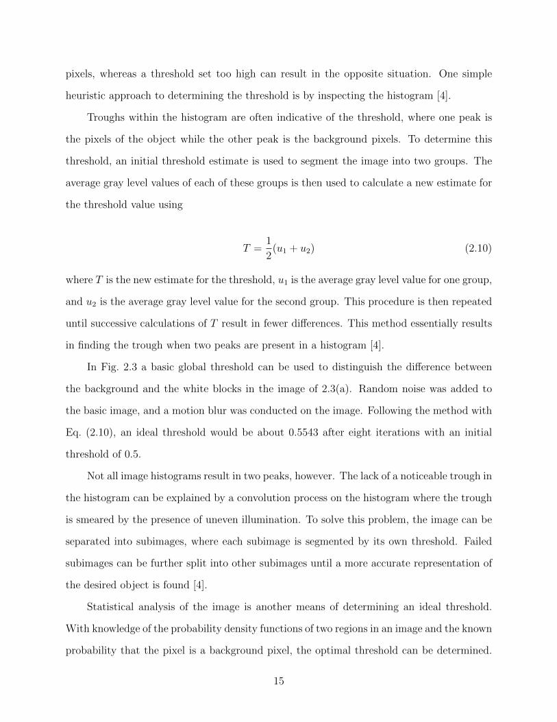
In Fig. 2.3 a basic global threshold can be used to distinguish the difference between

the background and the white blocks in the image of 2.3(a). Random noise was added to

the basic image, and a motion blur was conducted on the image. Following the method with

Eq. (2.10), an ideal threshold would be about 0.5543 after eight iterations with an initial

threshold of 0.5.

Not all image histograms result in two peaks, however. The lack of a noticeable trough in

the histogram can be explained by a convolution process on the histogram where the trough

is smeared by the presence of uneven illumination. To solve this problem, the image can be

separated into subimages, where each subimage is segmented by its own threshold. Failed

subimages can be further split into other subimages until a more accurate representation of

the desired object is found [4].

Statistical analysis of the image is another means of determining an ideal threshold.

With knowledge of the probability density functions of two regions in an image and the known

probability that the pixel is a background pixel, the optimal threshold can be determined.

15

(a) Original Image (b) Histogram of Image

Figure 2.3: Sample Image and Histogram

The threshold value for which the error of classifying a background pixel as an object pixel

is minimized using the following equation:

P1p1(T ) = P2p2(T ) (2.11)

where P1 is the probability of occurrence of one class of pixels, P2 is the probability of the

other class of pixels, p1 is the probability density function of the first class of pixels, p2 is

the probability density function of the second class of pixels, and T is the optimal thresh-

old. Under the assumption of Gaussian probability density functions, the total probability

density function can be characterized by the sum of the probability density functions of

the background and object pixels. The optimal threshold can be solved using the following

equation which arises from the knowledge of the variance σ2 and the mean µ:

AT 2 +BT + C = 0 (2.12)

16

where

A = σ21 − σ2

2 (2.13)

B = 2(µ1σ22 − µ2σ

21) (2.14)

C = σ21µ

22 − σ2

2µ22 + 2σ2

1σ22 ln

(σ2P1

σ1P2

)(2.15)

Solving the quadratic equation can result in a solution with two thresholds. If the variances

of each class of pixels are equal, then a single threshold is sufficient and the equation simplifies

to:

T =µ1 + µ2

2+

σ2

µ1 − µ2

(lnP2

P1

)(2.16)

If P1 = P2 or σ = 0, the optimal threshold is the average of the means, as explained above

[4].

Edge Detection

Edge detection is often used as a means of extracting features from an image. A simple

strategy for edge detection is the use of gradients to distinguish edges of features. A gradient

for an image f(x, y) is as follows:

∇f =

Gx

Gy

=

∂f∂x

∂f∂y

(2.17)

The gradient of an image is based on obtaining the partial derivatives of ∂f∂x

and ∂f∂y

for

each pixel in an image. Generally, a mask is created in order to compute the gradient at

each point in an image. The Roberts cross-gradient operators [4] are used to implement a

17

first-order partial derivative at a point and are as follows:

Gx = z9 − z5 (2.18)

Gy = z8 − z6 (2.19)

where z9 is the lower right index, z5 is the upper left index, z8 is the lower left index, and z6

is the upper right index in a 2 x 2 array. 3 x 3 matrix operations are more widely used for

gradient determination and include the Prewitt Eq. (2.20) and Sobel Eq. (2.21) masks for

the horizontal and vertical directions.

−1 −1 −1

0 0 0

1 1 1

−1 0 1

−1 0 1

−1 0 1

(2.20)

−1 −2 −1

0 0 0

1 2 1

−1 0 1

−2 0 2

−1 0 1

(2.21)

Several variations on these masks exist, such as that for detecting discontinuities in the

diagonal directions [4].

Canny [19] edge detection is a procedure for designing edge detectors for arbitrary edge

profiles. The detector uses adaptive thresholding with hysteresis to eliminate streaking of

edge contours. The thresholds are set according to the noise in the image, and several opera-

tor widths are used to deal with different signal-to-noise ratios. In addition, researchers have

developed a method for efficient generation of highly directional masks at several orientations

and their integration into a single description [19].

18

Hough Transform and Line Extraction

Edge detection creates images where, ideally, the edges of images are present as pix-

els while other features are ignored. Due to noise, breaks in the edge from nonuniform

illumination, and other spurious intensity discontinuities, the actual edges often have gaps.

Techniques called edge linking provide a means of rebuilding the edges using strength of the

response of the gradient operator and the direction of the gradient vector; thus each pixel is

calculated and linked points stored [4].

Another method to fill gaps involves linking points not by looking in the local area of

each point, but by determining first if they lie on a curve of a specified shape. By checking

each pair of points, a list of possible lines can be developed. The distance from each point

to each line is checked and points are allocated to each line. However, this strategy is

computationally intensive. The number of lines based on n points is n(n−1)2

with n(n(n−1))2

comparisons of every point to all lines. Unfortunately, this strategy is inappropriate for most

real-time applications [4].

The Hough transform [20] is a means of linking edges that avoids the aforementioned

computationally intensive procedure. Hough’s original patent was based on plotting the

parameters of point-slope form - namely, slope a and y-intercept b for the line equation

y = ax + b. Thus, in this plot a single line represents a coordinate point in x-y coordinate

space. The intersection of two lines in a-b space represents the parameters (a′, b′) for a line

that contains both corresponding points in x-y space for each intersecting line. Thus, every

line in a-b space that intersects at point (a′, b′) is a point on the line characterized by (a′, b′)

in x-y space [4].

The a-b parameter space is subdivided into accumulator cells within the expected range

of the slope and intercept values. For every point in the x-y plane, its parameter a equals each

of the allowed subdivision values on the a-axis and b is solved for using the point-slope form

of the line. If a choice of a results in the solution b, then the accumulator cell is incremented.

Cells with high values result in lines with many points. More subdivisions in the ab-plane

19

results in higher accuracy at the cost of higher computation time. The computation required

for the Hough transform involves nK computations, where n is the number of points and K

is the number of increments used to divide the a axis. Thus, this method has a much lower

computational complexity than checking each pair of points individually [4].

The problem with Hough’s original procedure for calculating the Hough transform is

that the slope approaches infinity as lines become more vertical. An alternative and more

generally accepted method for calculating the Hough transform is the use of the radial

descriptions ρ and θ rather than the slope-intercept parameters. The normal representation

of a line is

x cos θ + y sin θ = ρ (2.22)

Using these parameters and if θ exists over the interval [0, π], then the normal parameters for

a line are unique. Like Hough’s original procedure, every line in the x-y plane corresponds

to a unique point in the θ-ρ plane. Each point in the x-y plane corresponds to a sinusoidal

curve in the θ-ρ plane defined by

ρ = xi cos θ + yi sin θ (2.23)

where (xi,yi) is a point in the x-y plane. The θ-ρ plane curves intersect at colinear points in

the x-y plane. Similarly, points lying on the same curve in the θ-ρ plane correspond to lines

that intersect at the same point in the x-y plane [21].

Like Hough’s original transform, acceptable error in θ and ρ is user-defined and the θ-ρ

plane is divided into a grid. Each region in the grid is treated as a two-dimensional array of

accumulators. For each point (xi, yi) in the picture plane, the corresponding curve is entered

in the array by incrementing the count in each cell along the curve. Each cell then records

the total number of curves passing through it. Cells containing high counts correspond to

likely lines in the x-y plane. Computation to calculate the Hough transform grows linearly

20

with the number of figure points. When n is large compared to the number of values of

θ uniformly spaced from [0, π], the Hough transform is preferable to considering all lines

between n(n−1)2

pairs of points [21].

Figures 2.4 and 2.5 show a sample image and its Hough transform, respectively. The

presence of a vertical line with the Hough transform shows that the Hough algorithm used is

not Hough’s original procedure but the revised version using ρ and θ. Two lines are present

within Fig. 2.4 labeled A and B. The origin of this image is located at the top left corner of

the image with the positive axes pointing to the right and down.

Figure 2.4: Example Initial Image

Fig. 2.5 shows the Hough transform of Fig. 2.4. Each point on the lines in Fig. 2.4 creates

a sinusoidal line in Fig. 2.5. As the sinusoids intersect, the points in the Hough transform

become more brightly lit, which is the result of incrementing each bin in the accumulator.

The two brightly lit points in Fig. 2.5 labeled A and B correspond to the similarly-labeled

lines in Fig. 2.4. Since intersecting sinusoidal curves in Hough space correspond with colinear

points in x-y space, the brightly lit areas in Fig. 2.5 represent the lines. The location of the

21

brightly lit points in θ-ρ space corresponds to the location of the lines in the image. The

length of the lines, then, can be determined from the “wings” of the sinusoidal curves in the

Hough transform. Larger “wings” corresponds to longer lines in the x-y image. The location

of the brightly lit point A is at (0,49), and the corresponding line in x-y space must have a

θ of 0 and a normal distance from the origin of about 49. Line A in Fig. 2.4 obviously fits

this requirement. Similarly, the brightly lit point B corresponds to a θ of 45 degrees and a

ρ of 190. Line B corresponds to that ρ and θ.

Figure 2.5: Hough Transform of Initial Image

An extension to the well-studied Hough transform is the probabilistic Hough transform

[22]. In the voting process of the Hough transform, a limited number of polls can replace

the full scale voting for all edge points in an image. A small subset of the edge points can

often provide sufficient input to the Hough transform, thus reducing execution time at the

cost of negligible performance loss. The limit on how many edge points can be ignored as

inputs to the Hough transform is dependent on the application [22].

22

2.2 Lane Level Localization

2.2.1 Kalman Filter

The Kalman filter [23] is a well studied recursive algorithm for optimally estimating a

process with noisy measurements. The measurements are assumed to be zero-mean Gaussian

and white. Two stages are generally described as the steps in the Kalman filter — the time

update and the measurement update. The time update equations are as follows:

x−k = Axk−1 +Buk−1 (2.24)

P−k = APk−1AT +Q (2.25)

where A is the state transition matrix, B is the control input matrix, x−k is the estimate of

the state matrix after the time update, x−k−1 is the estimate of the state before the update,

P is the error covariance matrix, and Q is the process noise covariance. The time update

produces an estimate of the state after the time step and an estimate of the performance of

the estimate through the P matrix.

The measurement update equations are as follows:

Kk = P−k HT (HP−k H

T +R)−1 (2.26)

xk = x−k +Kk(zk −Hx−k ) (2.27)

Pk = (I −KkH)P−k (2.28)

where K is the Kalman gain, H is the measurement transition matrix, and I is the identity

matrix. The measurement update calculates the Kalman gain, which is used for weighting the

measurement residuals. An inaccurate measurement will be weighted less in the calculation

of the state estimate than a more accurate measurement. Hx−k is an estimate of the state

prior to a measurement, and zk is the measurement. Finally, the error covariance matrix P

is updated with knowledge of the Kalman gain.

23

For nonlinear systems, the Kalman filter is often modified into the extended Kalman

filter, which uses system models to project the state through each timestep in the time

update and the measurement estimate in the measurement update. The system model must

be known to approximate the nonlinear function for propagation into the next time step.

The equations for the time update in the extended Kalman filter are as follows:

x−k = f(xk−1, uk−1, 0) (2.29)

P−k = AkPk−1ATk +WkQk−1W

Tk (2.30)

where W is the process Jacobian.

For the measurement update, the equations are


T + VkRkVTk ))−1 (2.31)

xk = x−k +Kk(zk − h(x−k , 0)) (2.32)

Pk = (I −KkHk)P−k (2.33)

where V is the measurement Jacobian.

2.2.2 Differential GPS

Differential GPS provides better accuracy than GPS alone. Reducing measurement

errors and improving satellite geometry improves GPS position estimates. The worst error

sources are common for users who are in close proximity on the surface of the earth. These

errors also do not change quickly. Thus if the error in a local area is known, corrections

can be made to the receivers in that area. These corrections are known as differential

corrections. Signals from additional satellites provide more estimates for user position and

generally result in a better navigation solution. Pseudo-satellites, also known as pseudolites,

act as additional satellite signals to improve the position estimate [3].

24

Local-area differential GPS uses a reference station which receives GPS signals and

transmits the differential corrections for a local area. Maritime DGPS has a horizontal

positioning accuracy of 1 to 3 meters at a distance of 100 km from the reference station.

The Nationwide Differential GPS, or NDGPS, provides local area differential GPS over land

and currently covers at least 90% of the continental United States [3].

Wide-area differential GPS provides differential corrections over much larger areas such

as continents or oceans. Measurements from a network of reference stations are used to pro-

cess the measurement errors into their constituent parts. Each receiver can then determine

its corrections based on the position estimate of the unaugmented GPS. The Wide Area

Augmentation System (WAAS) broadcasts corrections to North America on L1 to provide

GPS position with an accuracy less than 10 meters [3].

Centimeter-level accuracy is possible using a reference station with a known location

within tens of kilometers from the receiver. This kind of accuracy is ideal for lane level

positioning at the cost of requiring carrier GPS measurements. Like all forms of GPS, line

of sight to the reference station and satellites is required. In difficult environments, such as

urban canyons or heavily forested areas, the reference stations and satellites may not have

line of sight to the receivers. Differential GPS, then, is not a reliable form of lane level

positioning in these difficult environments [3].

2.2.3 Inertial / Vision Sensor Fusion

A common strategy for combining inertial and visual sensors is the structure from motion

(SfM) problem. Structure from motion estimates the 3-D position of points in the scene with

respect to a fixed coordinate frame and the pose of the camera [16]. Features within the

image are tracked from frame to frame, and the change in camera pose and world coordinates

for each feature is estimated. These features can be either points [24] or lines [25]. Ansar

[26] presented a general framework for a linear solution to the pose estimation problem with

points and lines. For 3-D reconstruction, the range to each point must be known, since

25

slow moving objects nearby can appear to move at the same speed as far away fast moving

objects. The most common approach to this problem is the use of stereo vision, where the

differences in each image can be used to determine the distance to points in the image. For

a single camera, 3D motion estimation can be determined over the course of multiple frames

[27]. One limitation of an inertial/vision system using this technique is the need to track

features across multiple frames. If a feature is not present within successive images, tracking

fails and the system cannot estimate ego (self) motion. As such, most inertial/vision systems

have a limit with respect to motion at which they can operate. However, most applications

involving inertial and vision systems, such as that of a mobile robot or robotic arm, do not

approach this limit under normal conditions.

2.3 Conclusions

This chapter has presented an overview of methods and strategies used in the work in

this thesis but were not actively researched. The chapter began with an overview of navi-

gation sensors. GPS is discussed first and is followed with a description of gyroscopes and

accelerometers present within an IMU. GPS/INS systems and their complementary charac-

teristics are described. Vision systems, specifically those concerning lane departure warning

systems, are then discussed as well as the pinhole camera model. Various methods for lane

level localization are presented in the following section. The equations of the Kalman filter

are discussed next as a common strategy for determining lane level location, and differential

GPS is mentioned for its ability to obtain centimeter level accuracy. Finally, research in in-

ertial and vision sensor fusion is presented with a discussion of their complementary features

and several strategies used in vision / INS systems.

26

Chapter 3

Vision System

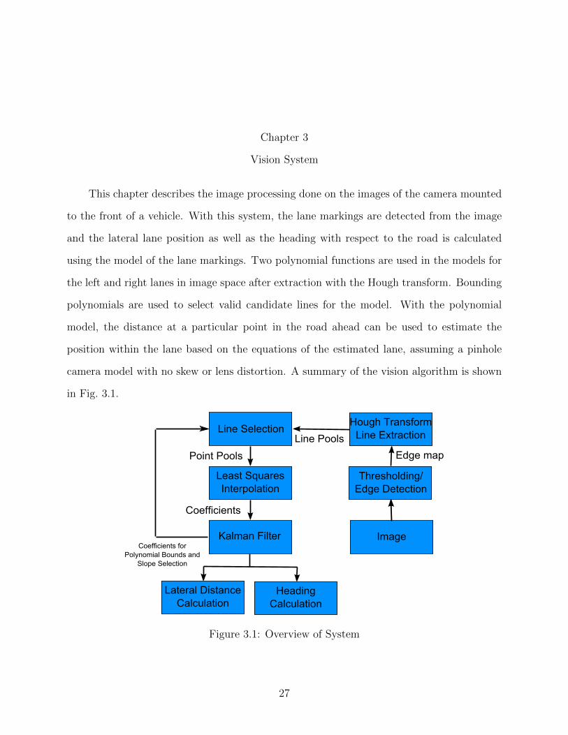
This chapter describes the image processing done on the images of the camera mounted

to the front of a vehicle. With this system, the lane markings are detected from the image

and the lateral lane position as well as the heading with respect to the road is calculated

using the model of the lane markings. Two polynomial functions are used in the models for

the left and right lanes in image space after extraction with the Hough transform. Bounding

polynomials are used to select valid candidate lines for the model. With the polynomial

model, the distance at a particular point in the road ahead can be used to estimate the

position within the lane based on the equations of the estimated lane, assuming a pinhole

camera model with no skew or lens distortion. A summary of the vision algorithm is shown

in Fig. 3.1.

Image

Thresholding/Edge Detection

Line SelectionHough Transform

Line Extraction

Least SquaresInterpolation

Lateral Distance Calculation

HeadingCalculation

Kalman FilterCoefficients for

Polynomial Bounds andSlope Selection

Edge map

Line Pools

Point Pools

Coefficients

Figure 3.1: Overview of System

27

The bounding polynomials reduce the effect of erroneous lines at far distances from the

current estimated line. Due to the necessity of nearby line detections, the detected lines from

the lane markings must not be far from the last estimated lane curve in the image. Assuming

smooth driving and a relatively high frame rate, the distance between the last estimated lane

curve and the new estimated lane curve should not increase significantly. This technique also

allows for the detection of road shape in the lane ahead, which can be useful for navigation

of autonomous vehicles, anticipation of future driver actions, or verification of the location

of the vehicle with maps. This technique does not currently extend beyond image space

and requires no other information other than the information from the frame image and the

calibration for the lateral distance measurement.

Another method for ignoring erroneous lines is to compare the slope of each individual

line with the slope of the estimated polynomial. Like the bounding polynomials, the slope

of each valid lane line does not change significantly from frame to frame. Each lane line is

then compared with the estimated lane in order to exclude erroneous lines that are contained

within the polynomial bounds.

A Kalman filter whose states are the coefficients of the polynomial for the estimated

lane marking is used in this research to reduce the impact of erroneous detected lane marking

lines. Some erroneous lane markings, such as those road exits, vegetation, and other objects

in the road, arise in individual frames and are not present in successive images. When these

erroneous lane marking estimations are detected, the Kalman filter reduces the impact of

these intermittent erroneous lane markings by filtering their effect on the current estimate

of the lane marking. However, lane tracking will be lost if the lane itself is unseen in the

image or if an erroneous object (such as the edge of a car or guardrail) is tracked as a lane

over successive images.

28

3.1 Lane Marking Line Selection

Typically the scene from a forward-looking camera consists of the road ahead. Much

of the image taken directly from the camera that does not include portions of the road has

been cropped, such as the sky and hood of the vehicle. Trees, other cars, guardrails, urban

sidewalks, and any feature in the image not pertaining to the lane markings is referred to as

noise in the image. Nevertheless, possible sources of noise are still present such as the grass

and edge of the forest. The quality of the estimate of the lane marking lines depends on the

ability to ignore these noise features and retain the actual lane marking lines.

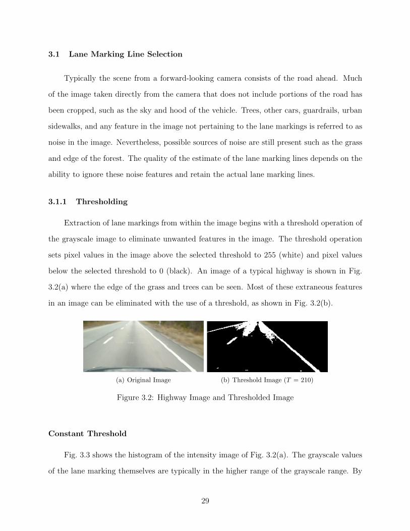
3.1.1 Thresholding

Extraction of lane markings from within the image begins with a threshold operation of

the grayscale image to eliminate unwanted features in the image. The threshold operation

sets pixel values in the image above the selected threshold to 255 (white) and pixel values

below the selected threshold to 0 (black). An image of a typical highway is shown in Fig.

3.2(a) where the edge of the grass and trees can be seen. Most of these extraneous features

in an image can be eliminated with the use of a threshold, as shown in Fig. 3.2(b).

(a) Original Image (b) Threshold Image (T = 210)

Figure 3.2: Highway Image and Thresholded Image

Constant Threshold

Fig. 3.3 shows the histogram of the intensity image of Fig. 3.2(a). The grayscale values

of the lane marking themselves are typically in the higher range of the grayscale range. By

29

setting the threshold within this higher range, the lane markings should be extracted from

the rest of the image, since lane markings are typically white or yellow. The selected constant

threshold is set just below the typical yellow value in a RGB color image at T = 210 to retain

both yellow and white lane markings. The resulting image of the road appears as white lines

over a black background, as seen in Fig. 3.2(b). For an ideal scenario, a constant threshold

provides good elimination of unwanted features while retaining the lane marking lines.

Figure 3.3: Intensity Image Histogram

However, different lighting conditions and environmental factors can eliminate the lane

marking lines from the image and create histograms in which a constant threshold will result

in thresholding which either eliminates the lane markings from the thresholded image or

eliminates the lane markings due to their inclusion as other features. Brightly lit scenes will

eliminate the lane marking lines from the thresholded image due to pixel values around the

lane markings being higher than the threshold, such as seen in the distance in Fig. 3.2(b)

where blobs mask the inner border lane marking.

Similarly, a poorly lit scene can eliminate the lane markings completely if the pixels

of the lane marking lines have grayscale values below that of the threshold. Fig. 3.4 is

30

one such example, where dusk reduces the brightness of the image and the lane markings

are not well illuminated except where the headlights shine, as shown in Fig. 3.4(a). Fig.

3.5 shows the histogram of the darker image in Fig. 3.4(a). The grouping of pixels in the

histogram are lower in grayscale value than that of the histogram of Fig. 3.3, and a smaller

fraction of pixels in the image has grayscale values above the threshold. As such, the actual

lane marking grayscale values are lower as well. The corresponding thresholded image with

the threshold value from the ideal condition of Fig. 3.2, T=210, results in the thresholded

image in Fig. 3.4(b), where the lane marking lines are almost completely eliminated. Since

the entire image has lower grayscale values, a lower threshold will extract the lane markings

well, but this value must be manually changed over the course of a long journey over different

lighting conditions or changed at the start of a short journey to compensate for the time

of day. Due to this problem, the constant threshold approach is not appropriate for robust

image processing in different lighting conditions.

(a) Darker Original Image (b) Threshold Image (T = 210)


Dynamic Threshold

Due to differences in lighting conditions throughout the day, a more dynamic threshold

is desired in order to capture the lane markings regardless of the illumination of the scene.

In the HSI color model, white lane markings have high intensity values but low saturation

values, as seen in Fig. 3.6. To extract white lines from the image, the saturation channel of

a color image is inverted, as seen in Fig. 3.6(d).

31

Figure 3.5: Intensity Image for Darker Image

This operation results in lane marking lines which are closer in value to the lane markings

present in the intensity channel. By averaging this inverted saturation channel and the

intensity channel, information beyond that of only the grayscale range is present in the new

image, as shown in Fig. 3.7(b).

The histogram of images changes significantly depending on the brightness and time

of day. To compensate for this problem, statistical values of the histogram can be used

to determine where the threshold can be set independent of the brightness conditions. A

simple low pass filter results in fewer anomalies in the image histogram; nevertheless, the

intensity image’s histogram does not have a peak which is easily determined. Fortunately,

the averaged inverted saturation and intensity image has a histogram with peaks that are

more pronounced in a much more Gaussian appearance, as shown in Fig. 3.8, compared with

the histogram of the intensity image in Fig. 3.3.

The following equation is used to determine the threshold value.

T = µ+Kσ (3.1)

32

(a) Original Image (b) Value channel

(c) Saturation channel (d) Inverted Saturation channel

Figure 3.6: Image Channels

(a) Original Image (b) Average of Inverted Saturation Chan-nel and Value Channel

Figure 3.7: Highway Image and Averaged Inverted Saturation and Value Image

where T is the threshold, µ is the mean of the image, σ is the standard deviation of the

image, and K is a value chosen based on the expected noise in the image. For Fig. 3.7(b), a

K value of 1.5 was chosen. With a mean of 196, a standard deviation of 33, and a K of 1.5,

the threshold is 245, and the resulting thresholded image is shown in Fig. 3.9(b). The blob

near the horizon in Fig. 3.2(b) has been removed while maintaining the presence of dashed

lane markings.

The darker image in Fig. 3.10(a) is tested with this system to analyze its performance

under different lighting conditions. Following the same procedure for the typical highway

image, the calculation for the threshold results in a threshold value of 182. This new threshold

creates a new thresholded image within which the lane markings are clearly visible, as shown

33

Figure 3.8: Average Image Histogram

(a) Original Image (b) Threshold Image


in Fig. 3.10. The constant threshold value which is ideal for the daytime image in Fig. 3.2(a)

eliminates the lane markings as shown in Fig. 3.4(b), which shows that the dynamic threshold

system outperforms that of the constant threshold system.

Despite this advantage in dealing with variable brightness in images, several factors can

cause problems during thresholding. Images with severe intensities, such as those images with

the sun as seen in Fig. 3.11, can cause the dynamic threshold to be set higher than desired,

thus eliminating the threshold from the image completely, as shown in Fig. 3.11(b). Certainly,

a new value of K in the threshold calculation would result in a better representation of the

lane markings in the thresholded image, as seen in Fig. 3.11(c). Although the blob from

34

(a) Darker Original Image (b) Threshold Image

Figure 3.10: Darker Highway Image and Dynamically Thresholded Image

the reflection of the sun is still present in the thresholded image of Fig. 3.11(c), the lane

markings are present. However, the need to change K during different lighting conditions

creates the same problems as that for a constant threshold.

(a) Bright Image with Sun (b) Threshold Image (K = 1.5)

(c) Threshold Image (K = 1)

Figure 3.11: Darker Highway Image and Dynamically Thresholded Image

3.1.2 Edge Detection

Following thresholding, an edge detection method is used to extract the edges of each

thresholded feature, or blob. The resulting image after edge detection appears as an outline

of the thresholded image, shown in Fig. 3.12. Several edge detection methods can be used

for this purpose, as shown in Fig. 3.12. The Laplacian of Gaussian method shown in Fig.

3.12(f) results in an edge map with larger blobs for the dashed lane marking in the far

35

distance. The Roberts edge detection method loses the sides of the solid right lane marking

in the far field, as shown in Fig. 3.12(e). Similarly, the Prewitt and Sobel edge detection

methods in Figures 3.12(d) and 3.12(c), respectively, have very little distance between the

two edges of the right lane marking, which can complicate detection of the lane marking lines

extracted using the Hough transform, which is discussed in 3.1.3. Canny edge detection was

determined to produce the best edge map of the system for lane tracking extraction with

ample space between the edges of the lane marking and adequate interpretation of the dashed

lane marking lines, as seen in Fig. 3.12(b).

(a) Original Image (b) Canny Edge Detection

(c) Sobel Edge Detection (d) Prewitt Edge Detection

(e) Roberts Edge Detection (f) Laplace Edge Detection

Figure 3.12: Various methods of edge detection

3.1.3 Line Extraction and Selection

One common feature extraction technique in lane departure warning systems is the use

of the Hough transform. The lines extracted from the Hough transform are representative

36

of all of the extracted features within the image. The Hough transform is conducted on the

edge map following edge detection, and the Hough lines, shown in Fig. 3.13 as red and blue

lines, are typically portions of the lines from edge detection. Every Hough line is classified

as either a left lane marking line or a right lane marking line. Lines corresponding to the

left lane marking are assumed to have a positive slope, while lines corresponding to the right

lane marking have a negative slope.

The lines detected through the Hough transform are not always the lane markings’

edges. To eliminate unwanted lines, two strategies are employed. One of these strategies uses

polynomial bounding curves, which reject lines based on their location within the image. The

other strategy uses slope comparison to eliminate lines based on their slope. Fig. 3.13 shows

the classification of lines as accepted as lane marking lines (blue) or rejected as extraneous

image features (red). For clarity, the following text describes both of these methods in

reference to a single lane marking.

Figure 3.13: Hough Lines

Polynomial Bounding Curves

The location of the lane from frame to frame (at 10Hz) does not change significantly in

a normal driving scenario. As such, the lines from the lane marking should be close within

the image to the last estimated lane marking. Two additional curves, called polynomial

bounding curves, for each lane marking are used as a means to bound the expected position

of the new lane marking within the image. These polynomial bounding curves are set at

a specific distance from the last estimated lane marking. Fig. 3.14 shows these polynomial

bounding curves as black lines offset from the estimated lane marking lines in yellow. As the

37

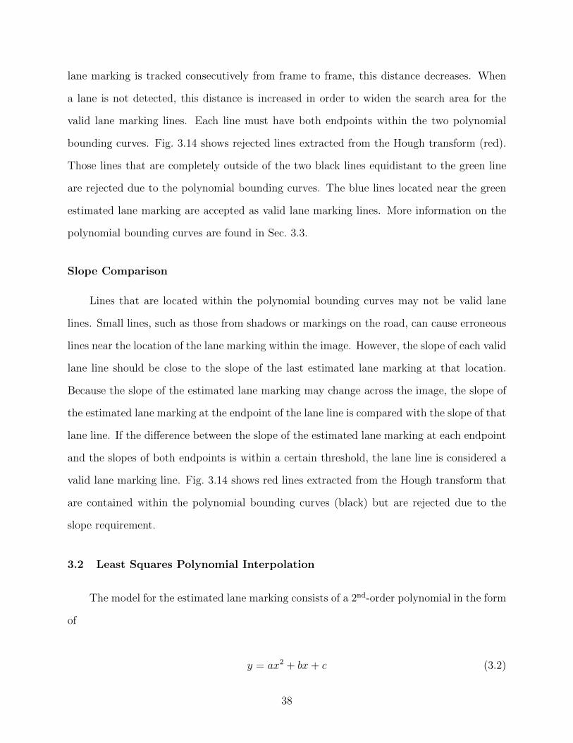
lane marking is tracked consecutively from frame to frame, this distance decreases. When

a lane is not detected, this distance is increased in order to widen the search area for the

valid lane marking lines. Each line must have both endpoints within the two polynomial

bounding curves. Fig. 3.14 shows rejected lines extracted from the Hough transform (red).

Those lines that are completely outside of the two black lines equidistant to the green line

are rejected due to the polynomial bounding curves. The blue lines located near the green

estimated lane marking are accepted as valid lane marking lines. More information on the

polynomial bounding curves are found in Sec. 3.3.

Slope Comparison

Lines that are located within the polynomial bounding curves may not be valid lane

lines. Small lines, such as those from shadows or markings on the road, can cause erroneous

lines near the location of the lane marking within the image. However, the slope of each valid

lane line should be close to the slope of the last estimated lane marking at that location.

Because the slope of the estimated lane marking may change across the image, the slope of

the estimated lane marking at the endpoint of the lane line is compared with the slope of that

lane line. If the difference between the slope of the estimated lane marking at each endpoint

and the slopes of both endpoints is within a certain threshold, the lane line is considered a

valid lane marking line. Fig. 3.14 shows red lines extracted from the Hough transform that

are contained within the polynomial bounding curves (black) but are rejected due to the

slope requirement.

3.2 Least Squares Polynomial Interpolation

The model for the estimated lane marking consists of a 2nd-order polynomial in the form

of

y = ax2 + bx+ c (3.2)

38

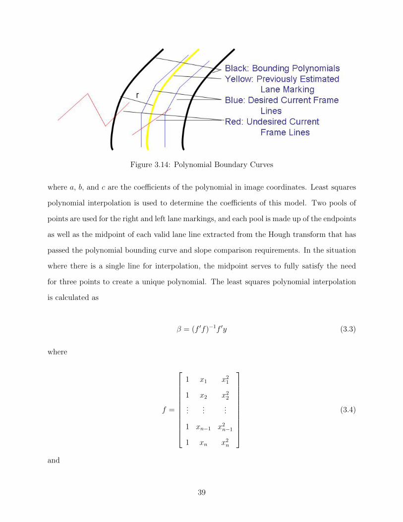
Figure 3.14: Polynomial Boundary Curves

where a, b, and c are the coefficients of the polynomial in image coordinates. Least squares

polynomial interpolation is used to determine the coefficients of this model. Two pools of

points are used for the right and left lane markings, and each pool is made up of the endpoints

as well as the midpoint of each valid lane line extracted from the Hough transform that has

passed the polynomial bounding curve and slope comparison requirements. In the situation

where there is a single line for interpolation, the midpoint serves to fully satisfy the need

for three points to create a unique polynomial. The least squares polynomial interpolation

is calculated as

β = (f ′f)−1f ′y (3.3)

where

f =

1 x1 x21

1 x2 x22...

......

1 xn−1 x2n−1

1 xn x2n

(3.4)

and

39

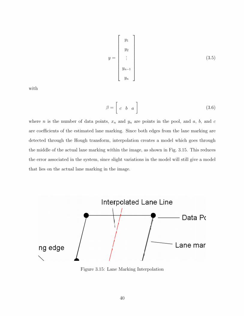
y =

y1

y2...

yn−1

yn

(3.5)

with

β =

[c b a

](3.6)

where n is the number of data points, xn and yn are points in the pool, and a, b, and c

are coefficients of the estimated lane marking. Since both edges from the lane marking are

detected through the Hough transform, interpolation creates a model which goes through

the middle of the actual lane marking within the image, as shown in Fig. 3.15. This reduces

the error associated in the system, since slight variations in the model will still give a model

that lies on the actual lane marking in the image.

Figure 3.15: Lane Marking Interpolation

40

3.3 Polynomial Boundary Curves

As previously mentioned, polynomial boundary curves, shown in Fig. 3.16 as the black

lines, are used to eliminate faulty lane marking lines from consideration into the lane estima-

tion using least squares interpolation. Each of these curves is calculated using the estimated

lane marking polynomial model by creating three sample points based on the lane marking

model and interpolating them into the 2nd order polynomials. The three sample points for

the right boundary curve are formed using the following equations:

xrb = xest + r sin(tan−1(2axest + b)) (3.7)

yrb = yest − r cos(tan−1(2axest + b)) (3.8)

where xrb is the x value of the desired point on the right side boundary curve, xest is the

x location of the point on the estimated lane marking curve, r is the normal distance from

the estimated lane marking curve to the boundary line, and a and b are coefficients of the

estimated lane marking curve. Similarly, the left boundary curve is calculated as follows:

xlb = xest + r sin(tan−1(2axest + b)) (3.9)

ylb = yest − r cos(tan−1(2axest + b)) (3.10)

where xlb is the x value of the desired point on the left side boundary curve and ylb is the

y value of the desired point on the left side boundary curve. Each point is normal to the

lane model at a certain distance from the estimated lane model. If consecutive lane lines

are found, this distance is decreased. If no lane lines are lost, this distance is increased to

expand the search area.

41

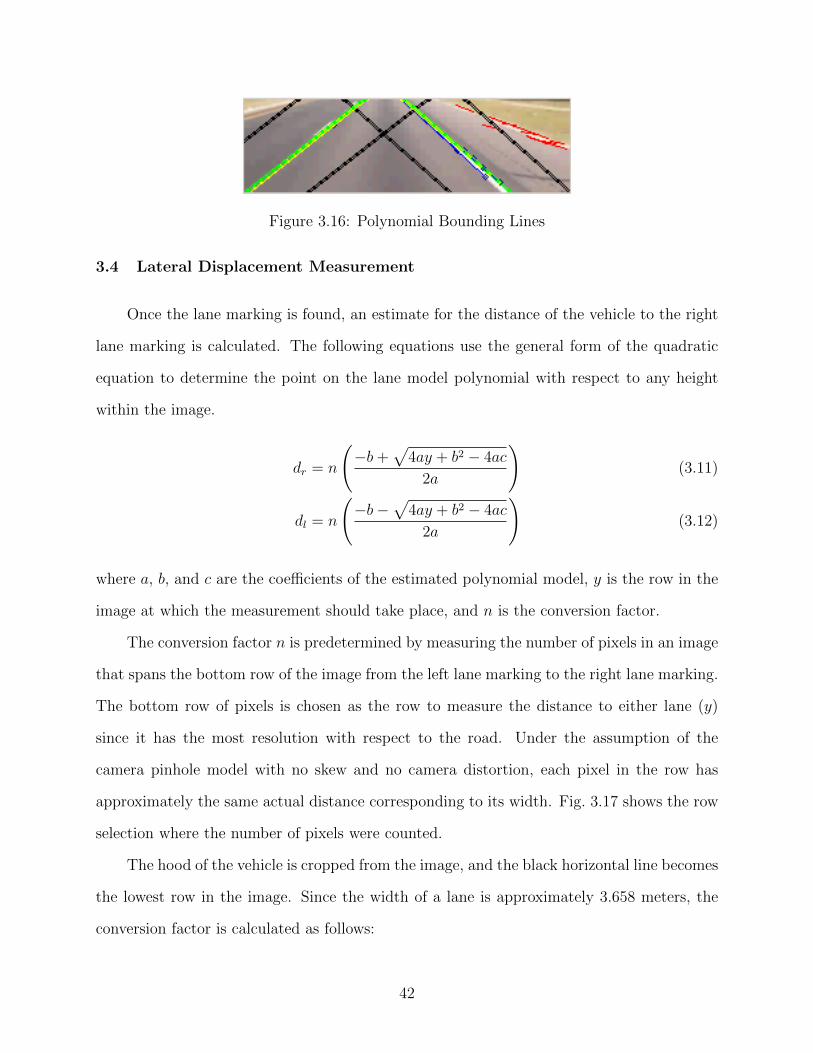
Figure 3.16: Polynomial Bounding Lines

3.4 Lateral Displacement Measurement

Once the lane marking is found, an estimate for the distance of the vehicle to the right

lane marking is calculated. The following equations use the general form of the quadratic

equation to determine the point on the lane model polynomial with respect to any height

within the image.

dr = n

(−b+

√4ay + b2 − 4ac

2a

)(3.11)

dl = n

(−b−

√4ay + b2 − 4ac

2a

)(3.12)

where a, b, and c are the coefficients of the estimated polynomial model, y is the row in the

image at which the measurement should take place, and n is the conversion factor.

The conversion factor n is predetermined by measuring the number of pixels in an image

that spans the bottom row of the image from the left lane marking to the right lane marking.

The bottom row of pixels is chosen as the row to measure the distance to either lane (y)

since it has the most resolution with respect to the road. Under the assumption of the

camera pinhole model with no skew and no camera distortion, each pixel in the row has

approximately the same actual distance corresponding to its width. Fig. 3.17 shows the row

selection where the number of pixels were counted.

The hood of the vehicle is cropped from the image, and the black horizontal line becomes

the lowest row in the image. Since the width of a lane is approximately 3.658 meters, the

conversion factor is calculated as follows:

42

Figure 3.17: Determining distance

n =wlpc

(3.13)

where n is the conversion factor, wl is the standard width of a lane or 3.658 meters, and pc

is the pixel count of the lane. The conversion factor n is then in units of meters per pixel

and can be multiplied with the corresponding pixel count on the bottom row of pixels to

determine lateral distance.

3.5 Heading Measurement

Following the approach of [28], the heading, ψ is determined from the camera based on

the vanishing point of the measured lane markings and the vanishing point of the camera.

The vanishing point of the measured lane markings is the point in the image where the lane

markings meet given a straight road. Parallel lines, such as lane markings, converge to the

43

vanishing point at the horizon. The vanishing point of the image is the location in the image

where the camera is perceived to point and is constant across each image given no change

in pitch. When a vehicle has a non-zero heading in the road, the vanishing point of the

camera is offset from the vanishing point of the image. The amount of offset can be used to

determine the heading in the image.

The vanishing point of the measured lane markings is based on the coefficients of the

polynomial lane marking model. The approach for determining the vanishing point when

two lane markings are detected is a simple determination of the intersection of the lane

markings. When a single lane is detected, the following formula is used to determine the

vanishing point in the image given a constant or assumed value for the horizon line:

Pl =−b+

√4ay + b2 − 4ac

2a(3.14)

Pr =−b−

√4ay + b2 − 4ac

2a(3.15)

where a, b, and c are the coefficients of the estimated polynomial model, Pl is the vanishing

point when only the left lane marking is detected, Pr is the vanishing point when only the

right lane marking is detected, and y is the known row in the image of the horizon line. Since

the vanishing point must be within the image, the determination for Pl or Pr is simple, the

polynomials for roads are very straight.

Fig. 3.18 shows the schematic with the lane markings, horizon, and vanishing points.

Point ~P1P2 represents the horizon, where P1 is the left boundary of the image on the horizon

line and P2 is the right boundary of the image on the horizon line. The distance ~OP

determines the relationship to the heading angle, ψ. To determine the heading, two pairs

of similar triangles are formed, where the center of projection is the common point between

the two triangles. One pair consists of a triangle with the center of projection as one of its

points and ~OP as its opposite side. The other triangle in the pair is the triangle formed at

infinite distance on the horizon, shown in Fig. 3.19 as ar, br, and cr.

44

POP1 P2image vanishing point lane marking vanishing point

Horizon Line

Lane

mar

king

Lane marking

M1 M2

Figure 3.18: Determining Heading

The second pair of similar triangles consists of a triangle whose point is once again

the center of projection but the opposite side is now an entire row in the image. The

corresponding other triangle is composed of dr, er, and fr in Fig. 3.19 and has an angle,

Θ known as the visual angle since it is the angle of view in the image. Notice that the

corresponding lines in the image plane for dr and fr are ~M1P1 and ~M2P2, as shown in Fig.

3.18. Right triangles are formed by dividing the similar triangles by r, which in turn divides

cr and er by two as shown in Fig. 3.19. The corresponding similar triangle for the image plane

divides a horizon line ~P1P2 into ~OP2. The relationship between the parallel lane marking

lines and the corresponding vanishing points in the image plane is based on equivalent ratios

in similar triangles and is shown in Eq. (3.16).

er2br2

=~OP

~OP2

(3.16)

45

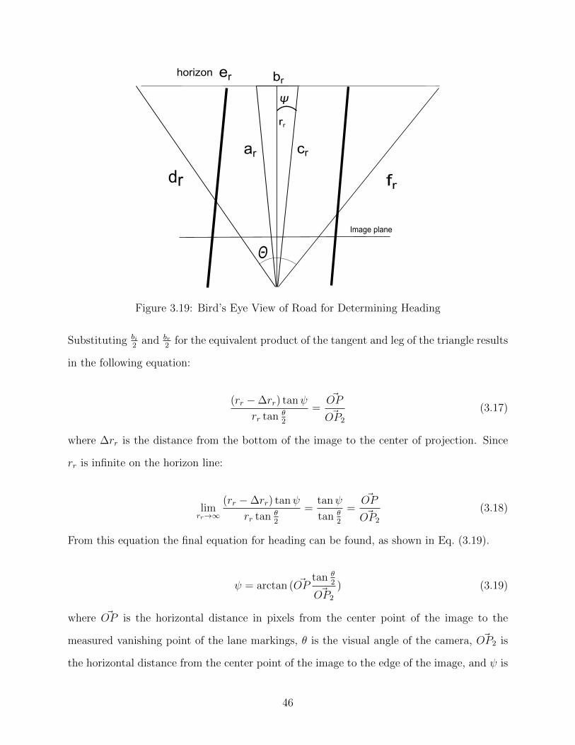
ψ

Θ

horizon

ar

br

rr

cr

dr

er

fr

Image plane

Figure 3.19: Bird’s Eye View of Road for Determining Heading

Substituting bi2

and br2

for the equivalent product of the tangent and leg of the triangle results

in the following equation:

(rr −∆rr) tanψ

rr tan θ2

=~OP

~OP2

(3.17)

where ∆rr is the distance from the bottom of the image to the center of projection. Since

rr is infinite on the horizon line:

limrr→∞

(rr −∆rr) tanψ

rr tan θ2

=tanψ

tan θ2

=~OP

~OP2

(3.18)

From this equation the final equation for heading can be found, as shown in Eq. (3.19).

ψ = arctan ( ~OPtan θ

2

~OP2

) (3.19)

where ~OP is the horizontal distance in pixels from the center point of the image to the

measured vanishing point of the lane markings, θ is the visual angle of the camera, ~OP2 is

the horizontal distance from the center point of the image to the edge of the image, and ψ is

46

the heading angle. Point O is the vanishing point of the image, and point P is the vanishing

point for the lane markings.

One drawback of the heading measurement is the requirement that the lane marking

lines be fairly straight. Since the measurement relies on the assumption that the vanishing

point of the lane markings corresponds to a point on the road axis with which to base the

measurement of the heading, a curved road will shift the vanishing point of the lane marking

away from the road frame. Future work is required to modify the algorithm to determine

the heading on a curved road.

3.6 Linear Kalman Filter

As explained earlier, lane marking lines from the Hough transform that are considered

valid and match both the location and slope requirements may not be real lane marking

lines. This is due to the fact that objects on the road which lie parallel to and near the

lane marking line may be detected as lane marking lines. Also, failure to fully detect the

lane marking lines can create groupings of points for interpolation that create erroneous lane

marking models.

To compensate for these error sources, a linear Kalman filter has been created which

filters coefficient measurements from the camera. Details of the Kalman filter can be found

in Sec. 2.2.1. The states of the filter are as follows:

x =

[aL bL cL aR bR cR

]T(3.20)

Both the A and H matrices are merely 6x6 eye matrices due to the lack of dynamics

in the system and the simple filtering purpose of the algorithm. Alternatively, a weighted

least squares algorithm would serve the same purpose. The coefficient states are initialized

so that the estimated lane model lies close to the typical location of the image in a regular

highway driving environment. The measurement covariance noise matrix, R, is as follows:

47

R =

σ2a 0 0 0 0 0

0 σ2b 0 0 0 0

0 0 σ2c 0 0 0

0 0 0 σ2a 0 0

0 0 0 0 σ2b 0

0 0 0 0 0 σ2c

(3.21)

Values chosen for σ2a, σ

2b , and σ2

c are provided in Appendix B.1. Modifying these values

changes the rate at which the lane marking model shifts within the image to the lane model

determined from polynomial interpolation.

The process covariance noise matrix, Q, is as follows:

R =

0.001 0 0 0 0 0

0 0.001 0 0 0 0

0 0 0.001 0 0 0

0 0 0 0.001 0 0

0 0 0 0 0.001 0

0 0 0 0 0 0.001

(3.22)

Due to the lack of dynamics in the system, the time update of the filter merely propagates

the current states and updates the P matrix. The time update equations are shown in Eqns.

(3.23) and (3.24).

x−k = Axk−1 (3.23)

P−k = APk−1AT +Q (3.24)

where A is the state transition matrix, B is the control input matrix, x is the estimate of

the state matrix after the time update, x is the estimate of the state before the update, P

is the error covariance matrix, and Q is the process noise covariance.

48

The measurement update calculates the gain K and compares the estimate of the state

with the measurement to generate a new state estimate. The P matrix is then once again

updated with the gain K and new P matrix. The equations for the measurement update

are listed in Equations (3.25-3.27).


T +R)−1 (3.25)

xk = x−k +Kk(zk −Hx−k ) (3.26)

Pk = (I −KkH)P−k (3.27)

The Kalman filter reduces the impact of erroneous lane curve measurements or shifts of the

polynomial model within the image. Results will be shown in Sec. 3.8.1.

3.7 Performance in Different Environments

The performance of the vision algorithm can change significantly depending on the

ability of the lane markings to be seen in the camera image, the time of day, and the

weather. This section describes some advantages and disadvantages of the vision system in

various environments. Numerical results can be found in Sec. 3.8.

3.7.1 Performance under Varying Lighting Conditions

Due to the various lighting scenarios that occur while a vehicle is on the road, a robust

vision system is desired for lane tracking. Sec. 3.1.1 has already discussed some aspects of

how lighting conditions effect the vision system. Fig. 3.20 shows a night scene with traffic

and overhead street lights. The lights from ongoing traffic, shown in Fig. 3.20(a) flushes out

the lane markings similar to the sun’s effect on the image as described in Sec. 3.1.1, and

the system fails in detecting the lane, as shown by the lack of lines in the edge map in Fig.

3.20(b). The glare from the headlights is shown as a circular blob in the edge map. The

other features in the edge map are primarily from the vehicle ahead and its brake lights.

49

(a) Night Scene (b) Night Scene Edge Map

Figure 3.20: Night Scene and Edge Map

Another night scenario where no street lights are shown and no oncoming traffic is shown

in Fig. 3.21. This image was taken on the National Center for Asphalt Technology (NCAT)

test track. As seen in Fig. 3.21(b), the lane markings are shown within the illumination of the

headlights. Unfortunately, the headlights also create another blob at the center of the image

where the illuminated ground is bright enough to exceed the threshold for thresholding.

Typically, circular blobs like the one shown in Fig. 3.21(b) do not impact the system other

than preventing features from being seen. Since the Hough transform is searching for lines

rather than curves, rarely will a line be extracted from the blob. When desired features are

outside of these blobs, the vision system can ignore the blobs and track the desired features.

(a) Night Scene at the Track (b) Night Scene at the Track Edge Map

Figure 3.21: Night Scene at the Track and Edge Map

Twilight has its own difficulties as well. With the sun so low in the sky, the image

may detect either the sun or bright flashes of sun, as seen in Fig. 3.22, which prevents lane

tracking. Commercial LDW systems will actually turn off in the presence of the sun in the

image due to the difficulty in detecting lanes.

50

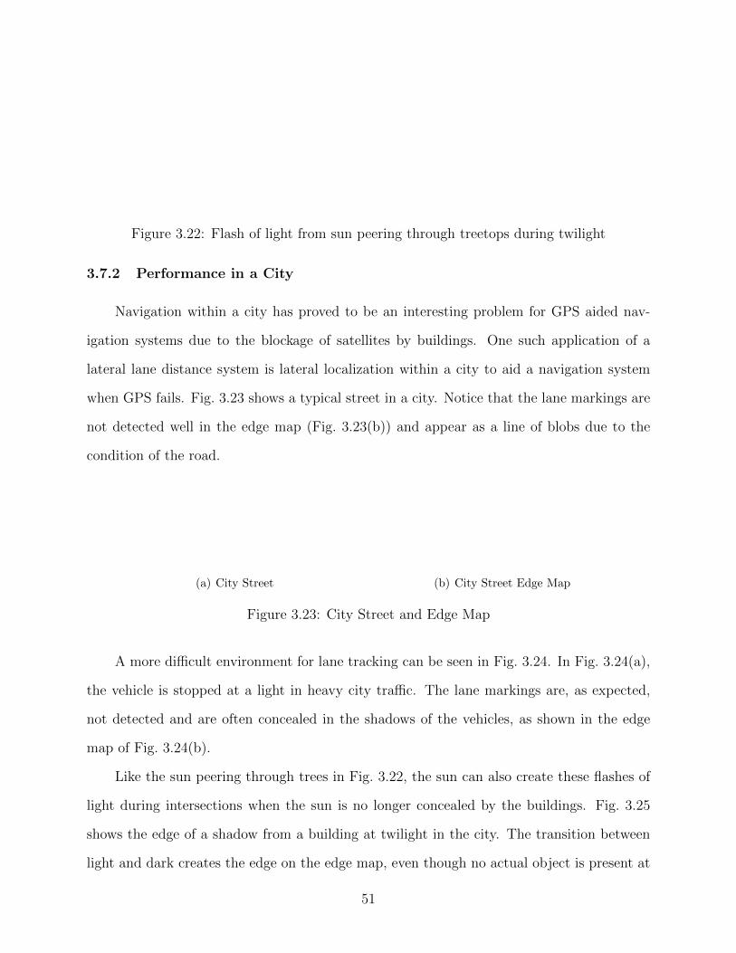
Figure 3.22: Flash of light from sun peering through treetops during twilight

3.7.2 Performance in a City

Navigation within a city has proved to be an interesting problem for GPS aided nav-

igation systems due to the blockage of satellites by buildings. One such application of a

lateral lane distance system is lateral localization within a city to aid a navigation system

when GPS fails. Fig. 3.23 shows a typical street in a city. Notice that the lane markings are

not detected well in the edge map (Fig. 3.23(b)) and appear as a line of blobs due to the

condition of the road.

(a) City Street (b) City Street Edge Map

Figure 3.23: City Street and Edge Map

A more difficult environment for lane tracking can be seen in Fig. 3.24. In Fig. 3.24(a),

the vehicle is stopped at a light in heavy city traffic. The lane markings are, as expected,

not detected and are often concealed in the shadows of the vehicles, as shown in the edge

map of Fig. 3.24(b).

Like the sun peering through trees in Fig. 3.22, the sun can also create these flashes of

light during intersections when the sun is no longer concealed by the buildings. Fig. 3.25

shows the edge of a shadow from a building at twilight in the city. The transition between

light and dark creates the edge on the edge map, even though no actual object is present at

51

(a) City Stoplight (b) City Stoplight Edge Map

Figure 3.24: City Stoplight Image and Edge Map

that location in the image. Also, once the vehicle get closer to the lit portion of the road,

the threshold will exceed the 255 grayscale value due to the dynamic threshold, and the edge

map will have no edges.

(a) Building Shadows (b) Shadows created by Buildings at Intersection

Figure 3.25: Shadows Created by Buildings at Intersections

Cities are difficult environments for lane detection systems. Lane markings are often

faint due to the difficulty in repainting them and lack of funds to do so. In addition, the

frequent stop and go traffic can cause erroneous tracking of other objects or blockage of the

lane markings by other vehicles. Fortunately, vehicle speeds in cities are usually low due

to congestion, and less speed means fewer fatalities. As such, most lane departure warning

systems are designed for highway scenarios and will not function below certain speeds.

3.7.3 Performance in Heavy Precipitation

Much like the performance of the vision algorithm in varying lighting conditions, the

lane markings in heavy rain are obscured from view. Heavy precipitation blocks the visibility

of the lane markings in the road. To account for this loss in visibility, drivers often slow their

speeds in order to more easily see the lane markings on wet roads. Similarly, the camera

52

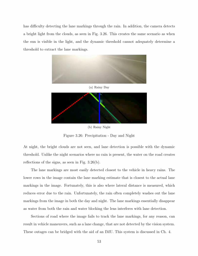
has difficulty detecting the lane markings through the rain. In addition, the camera detects

a bright light from the clouds, as seen in Fig. 3.26. This creates the same scenario as when

the sun is visible in the light, and the dynamic threshold cannot adequately determine a

threshold to extract the lane markings.

(a) Rainy Day

(b) Rainy Night

Figure 3.26: Precipitation - Day and Night

At night, the bright clouds are not seen, and lane detection is possible with the dynamic

threshold. Unlike the night scenarios where no rain is present, the water on the road creates

reflections of the signs, as seen in Fig. 3.26(b).

The lane markings are most easily detected closest to the vehicle in heavy rains. The

lower rows in the image contain the lane marking estimate that is closest to the actual lane

markings in the image. Fortunately, this is also where lateral distance is measured, which

reduces error due to the rain. Unfortunately, the rain often completely washes out the lane

markings from the image in both the day and night. The lane markings essentially disappear

as water from both the rain and water blocking the lens interferes with lane detection.

Sections of road where the image fails to track the lane markings, for any reason, can

result in vehicle maneuvers, such as a lane change, that are not detected by the vision system.

These outages can be bridged with the aid of an IMU. This system is discussed in Ch. 4.

53

3.8 Experimental Results - Vision System

The experimental results from the vision algorithm were conducted to determine the

accuracy of the lateral distance and heading measurements from the vision algorithm only.

In this test run, a Hyundai Sonata was equipped with a forward-looking camera that was

mounted on a conventional roof rack. The Sonata was driven on the right lane around the

full extent of the NCAT test track to simultaneously acquire RTK GPS coordinates and

frame grabs from the camera. Each distance from the camera images was compared with

the truth measurements from GPS to determine the accuracy of the system. Methodology

for obtaining truth data can be found in Appendix A. The accuracy of the coefficient states

can be seen by visual inspection. Simply, if the polynomial models lie on the lane markings

in the images, then the coefficients are being estimated correctly. In this test run, the quality

of the lane markings is not ideal - the lane markings disappear on some segments of the track

and are faint in others. As such, in several frames, no lane marking is detected. Also, at

one part of the track the asphalt creates a distinct line between light colored asphalt and

dark colored asphalt that is near the dashed left lane markings, and the left lane marking

estimate tracks this line.

3.8.1 Polynomial Coefficient State Estimation

Each of the coefficient states are estimated through the measurement update using the

polynomial coefficients obtained by the vision algorithm. The Kalman filter of the vision

system reduces the effect of any erroneous or noisy polynomial model coefficients. Fig. 3.27

shows the coefficient b of the right lane polynomial, and Fig. 3.28 shows the coefficient c of

the right lane polynomial for frames in which the right lane markings were detected. The lane

models failed to pass the requirement for 2nd-order interpolation (as explained in Appendix

B.1) and so the a coefficient remained at zero throughout the run. The effect of the Kalman

filter in both graphs is easily seen.

54

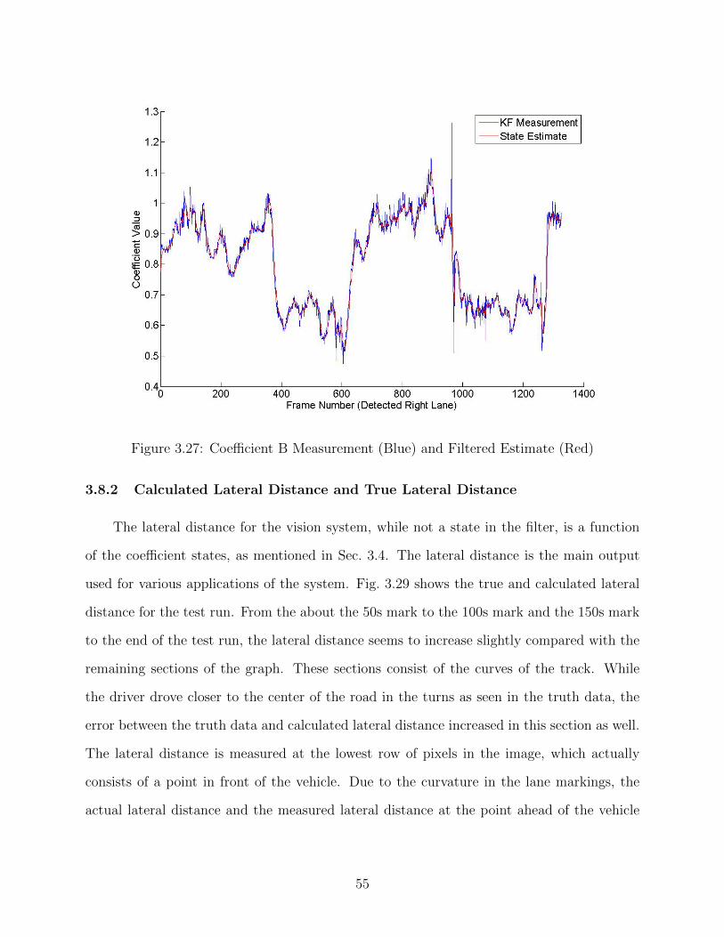
Figure 3.27: Coefficient B Measurement (Blue) and Filtered Estimate (Red)

3.8.2 Calculated Lateral Distance and True Lateral Distance

The lateral distance for the vision system, while not a state in the filter, is a function

of the coefficient states, as mentioned in Sec. 3.4. The lateral distance is the main output

used for various applications of the system. Fig. 3.29 shows the true and calculated lateral

distance for the test run. From the about the 50s mark to the 100s mark and the 150s mark

to the end of the test run, the lateral distance seems to increase slightly compared with the

remaining sections of the graph. These sections consist of the curves of the track. While

the driver drove closer to the center of the road in the turns as seen in the truth data, the

error between the truth data and calculated lateral distance increased in this section as well.

The lateral distance is measured at the lowest row of pixels in the image, which actually

consists of a point in front of the vehicle. Due to the curvature in the lane markings, the

actual lateral distance and the measured lateral distance at the point ahead of the vehicle

55

Figure 3.28: Coefficient C Measurement (Blue) and Filtered Estimate (Red)

is slightly different. Therefore, the error in the system increases due to the curvature of the

lane markings.

The lateral distance error is seen in Fig. 3.30. The maximum error in the system on a

straightaway is about 20 cm. As mentioned previously, most of the error in Fig. 3.30 arises

in the turns of the track. The error is expected to increase if the vehicle maneuvered more

within the lane.

3.8.3 Calculated Heading and True Heading

The heading, like the lateral distance, is not a state in the filter but can be used as a

measure of the accuracy of the system. Unlike the lateral distance calculation, the heading is

not typically used as a judge of quality of the system due to sideslip. However, the heading is

needed in the EKF with the inertial inputs of the IMU in the vision/IMU section. Fig. 3.31

shows the heading calculation compared with truth. Like the lateral distance calculation, the

56

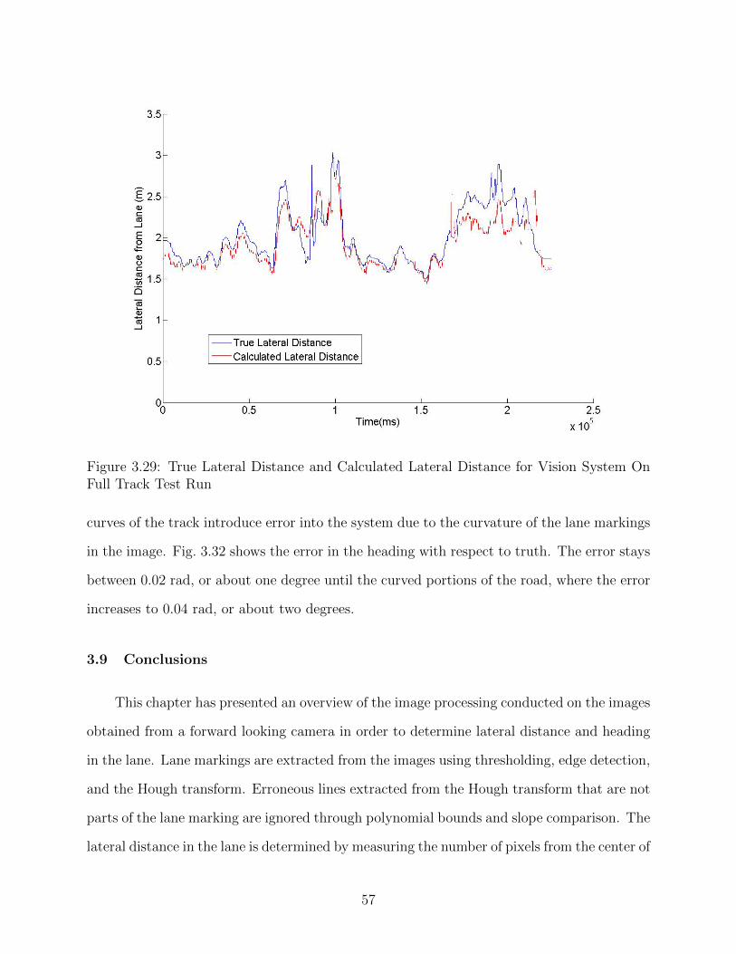
Figure 3.29: True Lateral Distance and Calculated Lateral Distance for Vision System OnFull Track Test Run

curves of the track introduce error into the system due to the curvature of the lane markings

in the image. Fig. 3.32 shows the error in the heading with respect to truth. The error stays

between 0.02 rad, or about one degree until the curved portions of the road, where the error

increases to 0.04 rad, or about two degrees.

3.9 Conclusions

This chapter has presented an overview of the image processing conducted on the images

obtained from a forward looking camera in order to determine lateral distance and heading

in the lane. Lane markings are extracted from the images using thresholding, edge detection,

and the Hough transform. Erroneous lines extracted from the Hough transform that are not

parts of the lane marking are ignored through polynomial bounds and slope comparison. The

lateral distance in the lane is determined by measuring the number of pixels from the center of

57

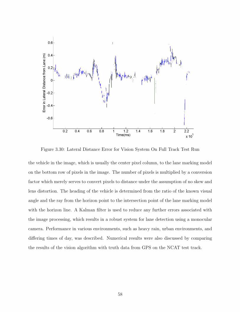
Figure 3.30: Lateral Distance Error for Vision System On Full Track Test Run

the vehicle in the image, which is usually the center pixel column, to the lane marking model

on the bottom row of pixels in the image. The number of pixels is multiplied by a conversion

factor which merely serves to convert pixels to distance under the assumption of no skew and

lens distortion. The heading of the vehicle is determined from the ratio of the known visual

angle and the ray from the horizon point to the intersection point of the lane marking model

with the horizon line. A Kalman filter is used to reduce any further errors associated with

the image processing, which results in a robust system for lane detection using a monocular

camera. Performance in various environments, such as heavy rain, urban environments, and

differing times of day, was described. Numerical results were also discussed by comparing

the results of the vision algorithm with truth data from GPS on the NCAT test track.

58

Figure 3.31: True Heading and Measured Heading for Vision System On Full Track TestRun

Figure 3.32: Heading Error for Vision System On Full Track Test Run

59

Chapter 4

Vision/Inertial System

This chapter describes the implementation of the inertial/vision system for tracking

lane marking lines and the vehicle’s location within the lane. A camera system can track the

lane markings well in ideal conditions. However, vision-only lane departure warning systems

are limited by the quality of the frame image and the information contained within each

frame. Objects on the road and other vehicles can lead to faulty tracking due to detection

of features similar to road markings. Additional road markings on the ground, such as that

of a crosswalk, turn arrow, or merged lane, can introduce rogue lines into the image and

shift the estimated lines beyond that of the actual lane markings. Blurry frames, adverse

weather conditions, faint lane markings, and shadows can ruin detection of lines. Dashed

lane markings from the center of the road can reduce the lane marking detection rate and

lead to gaps in the tracking of the lane model. Other vehicles on the road, especially in an

urban environment, and faint road markings can interfere with tracked lane markings. The

addition of inertial data into the system can fill in the gaps when vision fails to track the

lane marking lines.

4.1 System Overview

A loosely coupled approach has been implemented which adds the inputs of an inertial

measurement unit (IMU) to an extended Kalman filter (EKF) for determining the lateral

distance within the lane even when vision measurements, specifically heading ψ and lateral

distance d, are not available. Fig. 4.1 shows the overall vision / inertial system. The Kalman

filter from the vision system is used to generate the lateral distance, d, and heading, ψ, as

60

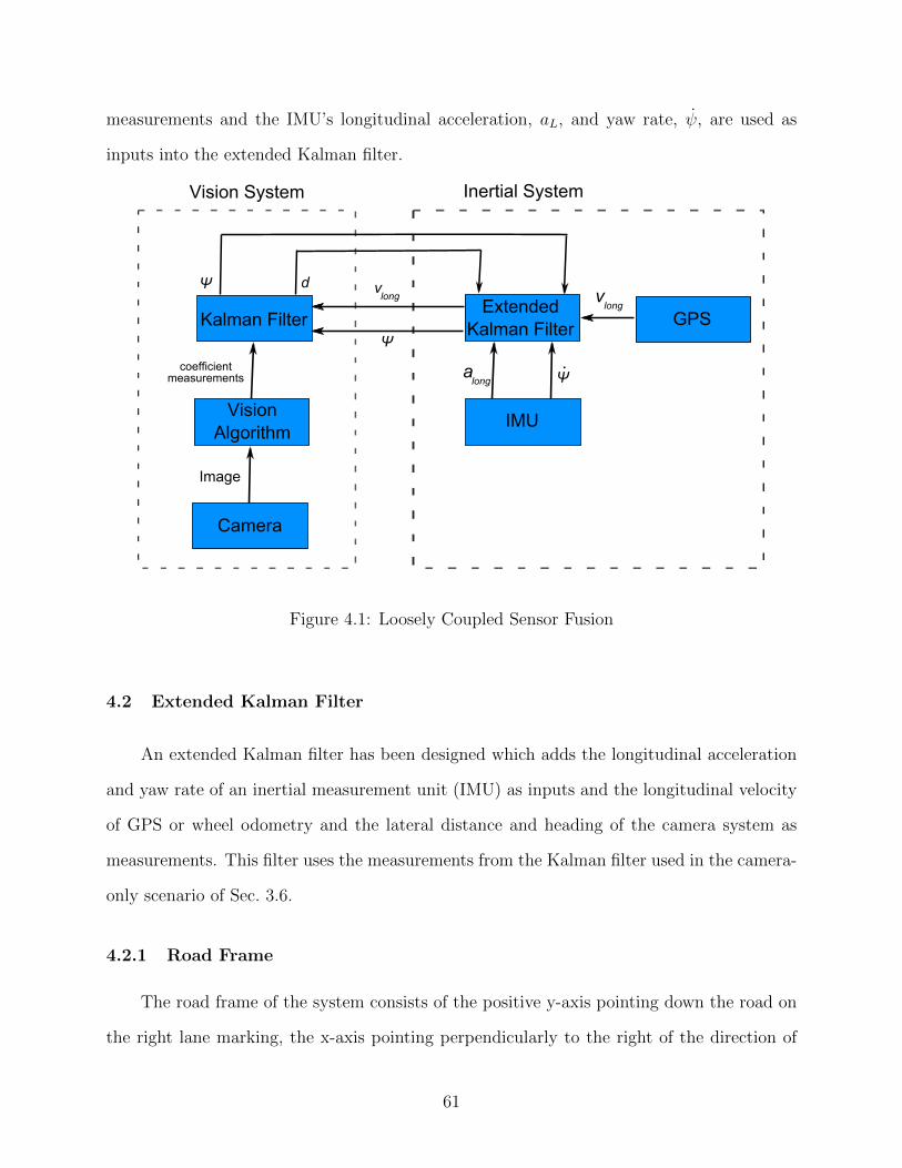
measurements and the IMU’s longitudinal acceleration, aL, and yaw rate, ψ, are used as

inputs into the extended Kalman filter.

Kalman Filter

coefficient measurements

dΨ

ExtendedKalman Filter

Vision Algorithm

Camera

IMU

Vision System Inertial System

Ψ.a

long

Image

vlong

Ψ

GPSvlong

Figure 4.1: Loosely Coupled Sensor Fusion

4.2 Extended Kalman Filter

An extended Kalman filter has been designed which adds the longitudinal acceleration

and yaw rate of an inertial measurement unit (IMU) as inputs and the longitudinal velocity

of GPS or wheel odometry and the lateral distance and heading of the camera system as

measurements. This filter uses the measurements from the Kalman filter used in the camera-

only scenario of Sec. 3.6.

4.2.1 Road Frame

The road frame of the system consists of the positive y-axis pointing down the road on

the right lane marking, the x-axis pointing perpendicularly to the right of the direction of

61

motion, and the z-axis pointing down and perpendicular to the road plane, as seen in Fig.

4.2. The distance py is the lateral displacement from the right lane marking and is typically

measured as a negative distance. As such, a positive distance measurement means that the

vehicle has driven off of the road.

Ψ

p

z

y

x

y

Figure 4.2: Road and Body Frame

4.2.2 Filter Structure

The states for the extended Kalman filter consist of the lateral distance py, the longi-

tudinal velocity vx, the longitudinal acceleration bias bx, the yaw ψ, and the yaw rate bias

bψ, as shown in Eq. 4.1.

62

x =

[py vx bx ψ bψ

]T(4.1)

These states were chosen to minimize the error associated with noise from the IMU

outputs and to minimize integration error. Other filter structures that were studied can be

found in Appendix C.

4.3 Time Update

The time update of the extended Kalman filter updates the vehicle states with the IMU

inputs. Additionally, the lateral velocity state is sent to the vision Kalman filter for updating

the lane marking model. The following section describes the time update for the EKF states

and Sec. 4.3.2 describes the velocity propogation to the vision Kalman filter for the time

update.

4.3.1 Continuous Update

Equations of Motion

The first time update equation consists of the propogation of the state estimate through

time.

x−k = f(xk−1, uk−1, 0) (4.2)

The function f is typically a group of nonlinear equations which uses the dynamics of the

system involved in the time domain to approximate the state at the new time k. Usually the

function results in dead reckoning of the system, where the inputs u and the previous state

xk−1 provide an estimate which is corrupted by error. The error in the estimate gradually

increases as time increases.

63

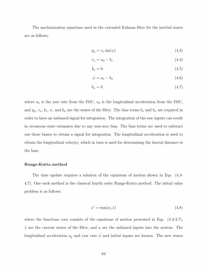
The mechanization equations used in the extended Kalman filter for the inertial states

are as follows:

py = vx sin(ψ) (4.3)

vx = u2 − bx (4.4)

bx = 0 (4.5)

ψ = u1 − bψ (4.6)

bψ = 0 (4.7)

where u1 is the yaw rate from the IMU, u2 is the longitudinal acceleration from the IMU,

and py, vx, bx, ψ, and bψ are the states of the filter. The bias terms bx and bψ are required in

order to have an unbiased signal for integration. The integration of the raw inputs can result

in erroneous state estimates due to any non-zero bias. The bias terms are used to subtract

out these biases to obtain a signal for integration. The longitudinal acceleration is used to

obtain the longitudinal velocity, which in turn is used for determining the lateral distance in

the lane.

Runge-Kutta method

The time update requires a solution of the equations of motion shown in Eqs. (4.3-

4.7). One such method is the classical fourth order Runge-Kutta method. The initial value

problem is as follows:

x′ = eom(u, x) (4.8)

where the functions eom consists of the equations of motion presented in Eqs. (4.3-4.7),

x are the current states of the filter, and u are the unbiased inputs into the system. The

longitudinal acceleration ay and yaw rate ψ and initial inputs are known. The new states

64

xk+1 is determined using the average of certain slopes, h1, h2, h3, h4, multiplied by the time

interval ∆t.

xn = xn−1 +1

6∆t(h1 + 2h2 + 2h3 + h4) (4.9)

tn = tn−1 + ∆t (4.10)

Each of the slopes h1, h2, h3, and h4 are determined as

h1 = eom(u, xk−1) (4.11)

h2 = eom

(1

2(uk − uk−1) + u, xk−1 +

1

2h1∆t

)(4.12)

h3 = eom

(1

2(uk − uk−1) + u, xk−1 + h2∆t

)(4.13)

h4 = eom(u, xk−1 + h3∆t) (4.14)

where u are the inputs to the system, the longitudinal acceleration ay and yaw rate ψ, xk−1

is the a priori estimate of the system, and eom are the differential equations of motion.

The slope of the function at the beginning of the interval from the known point xk−1 to the

unknown point xk is h1. The slope at the midpoint of the interval using the prior slope h1

to determine the value of x at the point un + 12∆t using Euler’s method is h2. Similarly, h3

is the slope at the midpoint using the slope h2. Finally, h4 is the slope at the end of the

interval using the value determined from h3. The slopes are averaged, where the slopes at

the midpoint are given more weight in the following manner:

H =1

6(h1 + 2h2 + 2h3 + h4) (4.15)

as seen in Eq. (4.9). With this method, the error in the system per step is on the order of

h5 with the accumulated error on the order h4.

65

The second step in the extended Kalman filter time update equations is the propagation

of the error covariance, P−k through time.

P−k = AkPk−1ATk +Q (4.16)

The error covariance P−k is implemented as a discrete matrix and determined by the

Jacobian matrix of the partial derivatives of the equations of motion with respect to x, as

follows:

A[i,j] =δf[i]δx[j]

(xk−1, uk−1, 0) (4.17)

The A matrix for the system, then, is as follows:

A =

1 ∆t sin(ψ) 0 vlong cos(ψ) 0

0 1 ∆t 0 0

0 0 1 0 0

0 0 0 1 ∆t

0 0 0 0 1

(4.18)

The Jacobian matrix A is calculated at each time step, and the process noise covariance

matrix Q is tuned after experimentation.

4.3.2 Vision System Time Update

The time update for the vision system in the combined INS/vision system is different

than that of the linear vision system alone. The discrete update of the linear Kalman filter

is used to propagate the coefficient states to the next time step. As described in Sec. 3.6, the

linear Kalman filter has no dynamics in the system, and the state transition matrix, A, is

merely an identity matrix with the same number of rows and columns as the number of states.

Knowledge of the system dynamics between images can provide an idea of the movement

66

of the lane marking model in the image plane. The linear Kalman filter’s time update can

be modified to account for any changes in the lane marking model between measurement

updates. This modification results in a nonlinear function which must be solved using an

extended Kalman filter.

For lane marking estimates with a small x2 coefficient a the equations for each coefficient

were determined from the change in the x coefficient b of the polynomial based on the lateral

velocity in the image. Small a values occur when the estimated lane marking polynomial

appears straight, such as the case when driving on a straight road. Due to the slope selection

criteria for determining valid lane markings, curved roads will results in high numbers of valid

lane marking lines in order to capture the curve of the road. When fewer valid lane markings

are present, a straight road can be assumed. For these situations, the a coefficient can be

assumed to be zero and a line model used.

The number of pixels shifted in image space is determined by

m =vx sin(ψ)∆t

n(4.19)

where n is the conversion factor from real to image space, vx is the estimated longitudinal

velocity from the EKF, ∆t is the time step, and m is the number of pixels in the horizontal

shift. Since the conversion factor n only applies to the bottom (or closest to the vehicle)

row in the image, the horizontal shift is based on this bottom row. Like the lateral distance

measurement from the camera, the bottom row of the image was chosen due to its projection

of the nearest location in the image and as such the most precise measurement in the image.

The equation for the straight line model is

y = bx+ c (4.20)

Since the slope of the line model changes based on the lateral distance in the image, the slope

term b should change, but the y-intercept should stay constant. The y-intercept represents

67

the vanishing point in the image, where all parallel lines converge. The linear lane model can

then be assumed to rotate around the vanishing point as the vehicle slides back and forth in

the lane.

The change in the slope of the linear lane model is a function of the shift of the road

in image space m and the rate at which the slope of the straight line model changes due to

perspective as that shift occurs. When the vehicle is directly over the lane marking, as is

the case when py = 0, the slope of the right lane model line is infinity. As the vehicle moves

laterally, the slope of the right lane model gradually decreases until the lane model aligns

with the horizon. The restriction of the image size and the knowledge that the lane marking

will never reach the horizon line due to other objects and the geometry of the lane itself

allows for the use of a conversion factor similar to the n conversion factor used in measuring

the lateral distance in the lane in Sec. 3.4. The equation for the number of radians per pixel,

r is then:

r =2q

w(4.21)

where w is the width of the image and q is the change in the slope in radians of the lane

marking model from the vertical lane marking line to the point at which the lane marking

line intercepts the edge of the image. This radial conversion factor can be multiplied with

the shift of pixels m to obtain the change in slope of the system.

The straight line model is rewritten to compensate for the change in image axes as

x =1

by − c

b(4.22)

Eq. (4.22) can then be written to shift the lane markings as

x =

(1

b− rm

)y − c

b(4.23)

Changing the function back to the standard y = bx+ c form results in the equation

68

y =b

1− brmx+

c

1− rmb(4.24)

This equation gives the new coefficients for the lane marking line model in image space after

the vehicle has moved laterally within the lane.

b =b

1− brm(4.25)

c =c

1− brm(4.26)

For situations where the road is not straight, a horizontal shift of the polynomial is

used for tracking the lane marking lines when measurement updates from the camera are

not available. The derivation for each coefficient change for a horizontal shift begins with

the equation for a horizontal shift of m pixels in the image.

y = a(x−m)2 + b(x−m) + c (4.27)

Each of the coefficient terms were collected in the following manner:

y = ax2 + (b− 2am)x+ (c+ am− bm) (4.28)

Thus the equations for the discrete update for each coefficient in the Kalman filter for the

horizontal shift of the vision system are as follows:

a = a (4.29)

b = b− 2am (4.30)

c = c+ am− bm (4.31)

Each updated coefficient is the coefficient of the new, horizontally shifted polynomial.

69

Equations (4.25)-(4.26) give the coefficients for a linear lane marking line after a lateral

displacement when the vanishing point of the camera and the vanishing point of the lane

marking lines do not shift in the image. Essentially the vehicle is sliding back and forth

within the lane. With a change in heading, the vanishing point of the image differs from the

vanishing point of the lane marking lines. This phenomenon is used in Sec. 3.5 to measure the

heading of the vehicle. Similarly, the change in heading can be counteracted by employing

Eqn. (3.19) to determine the shift of the vanishing point of the lane markings with respect

to the image plane. The shift in pixels of the lane marking vanishing point is

~OP =tan ψtan θ~OP2

(4.32)

where ~OP is the shift in pixels of the lane marking vanishing point, ψ is the change in

heading, θ is the visual angle of the camera, and ~OP2 is the width of half of the image. ~OP

can then be used in place of m in Eqns. (4.29-4.31) to shift the lane markings horizontally

to approximately coincide with the shift of the lane markings due to the change in heading.

Fig. 4.3 shows the changes in the coefficients during the time update for the Kalman

filter of the vision system for the linear lane model. The green line is the a priori lane

marking estimation line. This line’s slope is changed as shown by label 1 to become the red

line estimation. If the change in heading is significant, the next step, identified by label 2

in the figure, shifts the linear lane model to account for the change in the vanishing point

of the lane markings (the purple vertical line’s intersection with the horizon line) and the

vanishing point of the camera (the blue vertical line’s intersection with the horizon line).

Since the update rate of an IMU (about 50Hz) is greater than that of the camera (about

10Hz), the polynomial model can shift between measurement updates and appear to shift

slightly from frame to frame. This impact is more pronounced in situations where the camera

algorithm fails to detect a lane marking, and the estimated model can appear to move with

the missed lane markings. Since the region of interest for each lane marking lies between

70

Prior to shiftSlope shiftHeading shift

1

2

horizon

dash

ed la

ne m

arki

ng

solid lane marking

solid lane marking

Figure 4.3: Kalman filter time update coefficient change for the linear lane model

the polynomial bounding lines from the estimated lane marking model, the region of interest

will shift along with the lane model estimate. This allows for fast convergence and lane

identification when a lane marking can once again be detected by the vision algorithm.

The error covariance matrix P must also take into consideration the new dynamics of

the coefficients arising from the knowledge of the lateral velocity in the system. The Jacobian

matrix A incorporates this additional information in the computation of P , as shown in Eq.

(4.33).

71

A =

1 0 0 0 0 0

0 −1(1−bL∗r∗m)2

0 0 0 0

0 −cL(1−bL∗r∗m)

−cL(1−bL∗r∗m)2

0 0 0

0 0 0 1 0 0

0 0 0 0 −1(1−bR∗r∗m)2

0

0 0 0 0 −cR(1−bL∗r∗m)

−cR(1−bR∗r∗m)2

(4.33)

where r is the radians per pixel as described in Eqn. (4.21), m is the distance per pixel as

described in Eqn. (4.19), and A is the state transition matrix derived through the Jacobian

of the coefficient changes.

4.4 Measurement Update

The measurement update serves to correct the states of the filter from any errors ac-

cumulated during the time updates. The vision system updates the heading ψ and lateral

distance py states, while the velocity measurement updates the longitudinal velocity state,

vx. Bias states are not updated.

The H matrix relates the measurements to the states and is as follows:

H =

1 0 0 0 0

0 1 0 0 0

0 0 0 1 0

(4.34)

Each state, other than the bias terms, has a corresponding measurement. The measurement

noise covariance matrix R is as follows:

R =

σ2px 0 0

0 σ2vlong

0

0 0 σ2ψ

(4.35)

72

where σ2px is the variance of the lateral position measurement, σ2

vlongis the variance of

the longitudinal velocity measurement, and σ2ψ is the variance of the heading measurement

from the camera. The values used in the filter are listed in Appendix B.2.

The gain equation in the time update is


T + VkRkVTk ))−1 (4.36)

The state update equation is

xk = x−k +Kk(zk − h(x−k , 0)) (4.37)

The error covariance matrix, P , is updated as follows:

Pk = (I −KkHk)P−k (4.38)

4.5 Observability Analysis

A system is observable if its current state can be determined using the outputs. A

simple test for observability is if the observability matrix, O, shown below is full rank.

O =

C

CA

CA2

...

CAn−1

(4.39)

The A matrix for the extended filter is as follows:

73

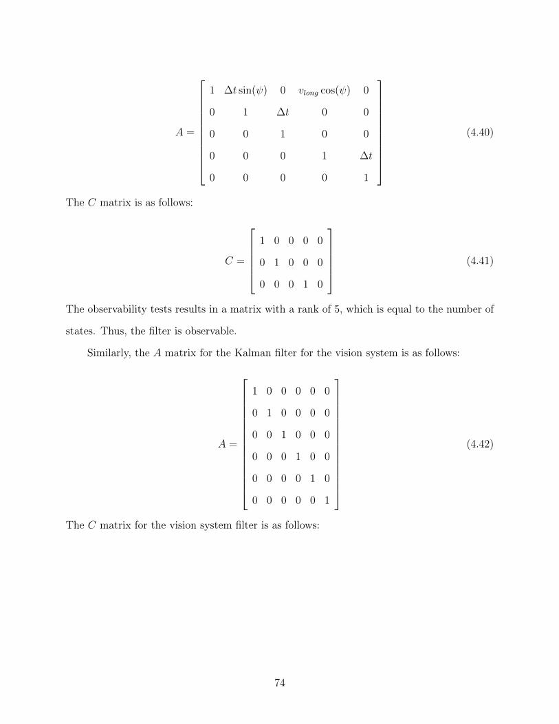
A =

1 ∆t sin(ψ) 0 vlong cos(ψ) 0

0 1 ∆t 0 0

0 0 1 0 0

0 0 0 1 ∆t

0 0 0 0 1

(4.40)

The C matrix is as follows:

C =

1 0 0 0 0

0 1 0 0 0

0 0 0 1 0

(4.41)

The observability tests results in a matrix with a rank of 5, which is equal to the number of

states. Thus, the filter is observable.

Similarly, the A matrix for the Kalman filter for the vision system is as follows:

A =

1 0 0 0 0 0

0 1 0 0 0 0

0 0 1 0 0 0

0 0 0 1 0 0

0 0 0 0 1 0

0 0 0 0 0 1

(4.42)

The C matrix for the vision system filter is as follows:

74

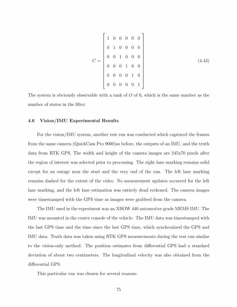
C =

1 0 0 0 0 0

0 1 0 0 0 0

0 0 1 0 0 0

0 0 0 1 0 0

0 0 0 0 1 0

0 0 0 0 0 1

(4.43)

The system is obviously observable with a rank of O of 6, which is the same number as the

number of states in the filter.

4.6 Vision/IMU Experimental Results

For the vision/IMU system, another test run was conducted which captured the frames

from the same camera (QuickCam Pro 9000)as before, the outputs of an IMU, and the truth

data from RTK GPS. The width and height of the camera images are 245x70 pixels after

the region of interest was selected prior to processing. The right lane marking remains solid

except for an outage near the start and the very end of the run. The left lane marking

remains dashed for the extent of the video. No measurement updates occurred for the left

lane marking, and the left lane estimation was entirely dead reckoned. The camera images

were timestamped with the GPS time as images were grabbed from the camera.

The IMU used in the experiment was an XBOW 440 automotive grade MEMS IMU. The

IMU was mounted in the center console of the vehicle. The IMU data was timestamped with

the last GPS time and the time since the last GPS time, which synchronized the GPS and

IMU data. Truth data was taken using RTK GPS measurements during the test run similar

to the vision-only method. The position estimates from differential GPS had a standard

deviation of about two centimeters. The longitudinal velocity was also obtained from the

differential GPS.

This particular run was chosen for several reasons:

75

• approximated straight road conditions of a highway

• taken at night under low light conditions

• faded section of lane markings

• double lane change maneuver

The straight road measurements are needed since the road frame is a non inertial road

frame. Due to the turns in a road, the IMU will detect changes in orientation, but the

road frame itself will not turn since the vehicle should always remain parallel to the lane

markings. To counteract this problem, the vision system would have to detect the curvature

of the road and rotate the measurements of the IMU. Due to the difficulties of detecting the

road curvature, this task is left for future work. All tests, then, are conducted on straight

roadways.

Low light conditions offer several problems as well as benefits, which were discussed in

Sec. 3.7.1. In this run, the low light reduces much of the noise associated with objects off of

the road. During the lane change maneuver, however, the vision system fails in tracking the

lanes as the vehicle moves toward the left lane despite the lane markings still being visible

in the image. If the test run been executed in the daylight, the vision algorithm could track

the lane marking until the lane marking went outside of the image boundaries.

The faded section of lane markings provides an idea of the drift of the IMU in the

system. With the dead reckoning from the IMU providing the lateral distance estimates,

the solution drifts away from truth. If the vision system fails to detect lane markings over a

significant period of time, the filter can report a lateral distance estimate that is outside of

the lane markings even though the vehicle is still between lane markings. The system must

periodically be updated with measurements in order to prevent this drift from occurring.

The double lane change maneuver shows the ability of the system to provide estimates

of lane position during dynamic maneuvers of the vehicle. During the lane change, the lane

markings are no longer detected. Following the lane change, the vehicle immediately changes

76

lanes back to the original lane. In a typical highway scenario with a lane departure warning

system, this maneuver represents a situation where the vehicle in the right lane wishes to

pass a vehicle in the left lane. However, the use of the turn signals would indicate to the

system that the lane change is intentional, and that the driver remains in control of the

vehicle.

The solution during the double lane change maneuver is solely based on the dead reck-

oning navigation from the IMU. In this scenario, a camera-only solution would fail to detect

the lane change as the lane markings fade as they lose the illumination of the headlights.

In addition, the vision only solution will report an erroneous lateral distance as the vehicle

travels in the left hand lane. Since their is no distinction in the vision system between the

left lane or the right lane, the solid left lane marking will provide a lateral lane measure-

ment. This lateral distance measurement will report the vehicle as in the right lane when

in actuality the vehicle is in the left lane. Therefore, a detected lane change without lane

markings tracked by the camera shows the greatest benefit of the vision/IMU system over

the camera-only solution.

4.6.1 Inputs and Bias Estimates

This section describes the inputs of the IMU into the time update of the extended

Kalman filter as well as the biases that act on those inputs. The inputs from the IMU must

capture the dynamics of the lane change maneuver while providing minimal drift error during

the lane marking outage in order to successfully track the lane markings. The Kalman filter

requires a zero mean input in order to function properly, and the bias state subtracts the

bias from the raw data to obtain a zero mean signal. Therefore, a well estimated bias term

results in a close to zero mean input signal.

77

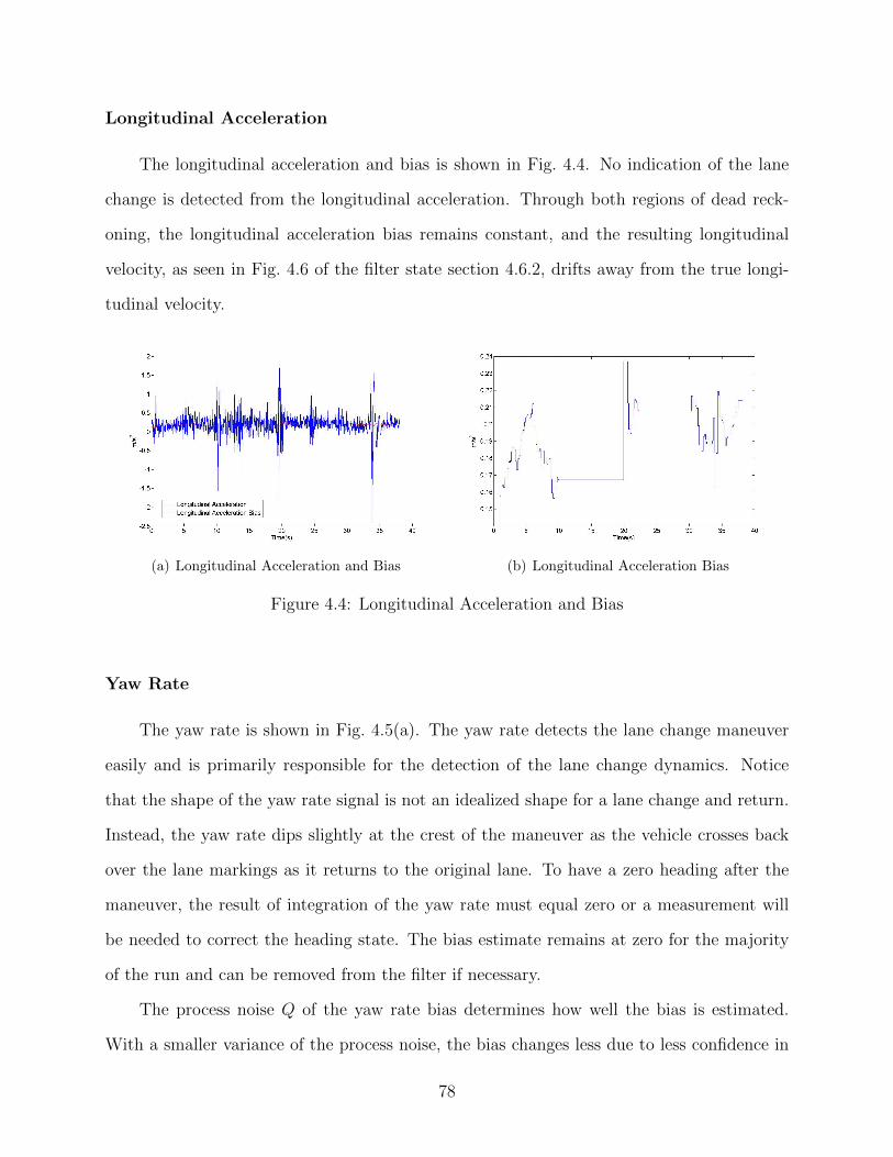
Longitudinal Acceleration

The longitudinal acceleration and bias is shown in Fig. 4.4. No indication of the lane

change is detected from the longitudinal acceleration. Through both regions of dead reck-

oning, the longitudinal acceleration bias remains constant, and the resulting longitudinal

velocity, as seen in Fig. 4.6 of the filter state section 4.6.2, drifts away from the true longi-

tudinal velocity.

(a) Longitudinal Acceleration and Bias (b) Longitudinal Acceleration Bias

Figure 4.4: Longitudinal Acceleration and Bias

Yaw Rate

The yaw rate is shown in Fig. 4.5(a). The yaw rate detects the lane change maneuver

easily and is primarily responsible for the detection of the lane change dynamics. Notice

that the shape of the yaw rate signal is not an idealized shape for a lane change and return.

Instead, the yaw rate dips slightly at the crest of the maneuver as the vehicle crosses back

over the lane markings as it returns to the original lane. To have a zero heading after the

maneuver, the result of integration of the yaw rate must equal zero or a measurement will

be needed to correct the heading state. The bias estimate remains at zero for the majority

of the run and can be removed from the filter if necessary.

The process noise Q of the yaw rate bias determines how well the bias is estimated.

With a smaller variance of the process noise, the bias changes less due to less confidence in

78

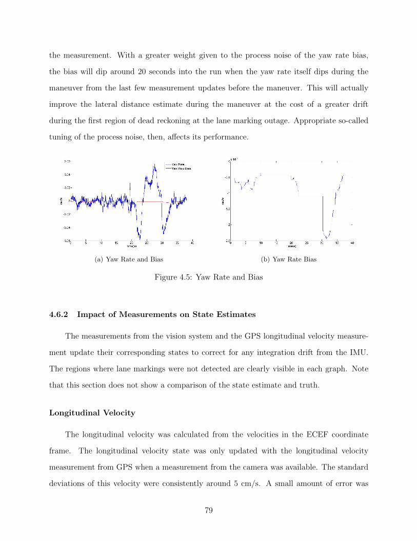
the measurement. With a greater weight given to the process noise of the yaw rate bias,

the bias will dip around 20 seconds into the run when the yaw rate itself dips during the

maneuver from the last few measurement updates before the maneuver. This will actually

improve the lateral distance estimate during the maneuver at the cost of a greater drift

during the first region of dead reckoning at the lane marking outage. Appropriate so-called

tuning of the process noise, then, affects its performance.

(a) Yaw Rate and Bias (b) Yaw Rate Bias

Figure 4.5: Yaw Rate and Bias

4.6.2 Impact of Measurements on State Estimates

The measurements from the vision system and the GPS longitudinal velocity measure-

ment update their corresponding states to correct for any integration drift from the IMU.

The regions where lane markings were not detected are clearly visible in each graph. Note

that this section does not show a comparison of the state estimate and truth.

Longitudinal Velocity

The longitudinal velocity was calculated from the velocities in the ECEF coordinate

frame. The longitudinal velocity state was only updated with the longitudinal velocity

measurement from GPS when a measurement from the camera was available. The standard

deviations of this velocity were consistently around 5 cm/s. A small amount of error was

79

introduced due to the presence of velocities in the vertical and lateral directions with respect

to the vehicle due to the calculation of the longitudinal velocity using the magnitude of the

total velocity in the ECEF frame.

vlong =√v2x + v2y + v2z (4.44)

Since the vehicle is primarily moving forward, the velocities in the vertical and lateral direc-

tions with respect to the vehicle should be very small.

The longitudinal velocity is shown in Fig. 4.6. During the test, the vehicle’s cruise control

was set to 30 miles per hour, or about 13 m/s. During the first lane marking outage, the

longitudinal velocity was corrected by the first measurement update after the lane markings

were detected, as seen by the drop in the graph at 20s from about 13.2 m/s to 12.7 m/s.

During the lane change maneuver, the dead reckoned estimate was closer to the measured

value around 30s into the test where the estimate of 13.1 m/s falls to only 13 m/s. During

the dynamic maneuver the longitudinal velocity was better estimated.

Heading

The heading measurements from the camera and the corresponding heading state are

shown in Fig. 4.7. The heading measurements are very noisy, and as such the variance in

the measurement covariance matrix is large. Therefore, the EKF does not weigh the heading

measurement from the camera much and mostly relies on inertial inputs from the IMU.

Notice, however, after the lane change maneuver that the camera heading measurement

does increase as the lane markings are detected before the vehicle ends the maneuver.

Lateral Distance

Probably the most important state from the filter is the lateral distance state since many

of the applications for this system, such as lane departure warning and lateral localization

systems, primarily use the lateral distance estimate. Due to the accuracy of the camera

80

Figure 4.6: Longitudinal Velocity Estimate vs. Measurement

lateral distance detection, the measurement can be trusted by the EKF and used to correct

the integration drift by the IMU. Fig. 4.8 shows the lateral distance measurements and the

estimated state. The estimated and measured lateral distance measurements are close as

expected until the measurement updates drop out during the lane marking outage, where

the estimate drifts away from the last measured lateral distance. Similarly, the estimate of

the lateral distance during the double lane change maneuver drifts away from the truth due

to integration error, as seen in 4.6.3.

4.6.3 Comparison with Truth

In order to determine how well the system works, the lateral distance and heading

estimates, px and ψ, were compared with truth values obtained using the methods presented

in Sec. 4.5(a). The truth for longitudinal velocity was essentially the same velocity used as

a measurement.

81

Figure 4.7: Heading Estimate and Measurement

Lateral Distance

Fig. 4.9 shows the lateral distance estimate compared with the truth for lateral distance.

The estimated solution remains close to truth except for the following three places: the region

where no lane markings were present from 10s to 20s, the lane change maneuver from 23s to

33s, and the exit to the skid pad at the NCAT test track where the lane markings disappear

from 36s to the end of the test. Each of these regions resulted in no camera measurements,

and dead reckoning from the IMU was used for lane estimation. As such the integration

drift is seen.

In Fig. 4.11, the error in the system with respect to truth is shown. Notice that the

error grows in the three regions of dead reckoning where no measurements from the camera

or GPS are presented. For the first dead reckoning region where the vehicle was moving

straight but no lane markings were detected, the drift resulted in error of about 60 cm. This

drift was small enough for the dead-reckoned estimate of the lane markings not to exceed

82

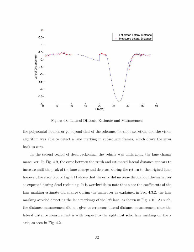
Figure 4.8: Lateral Distance Estimate and Measurement

the polynomial bounds or go beyond that of the tolerance for slope selection, and the vision

algorithm was able to detect a lane marking in subsequent frames, which drove the error

back to zero.

In the second region of dead reckoning, the vehicle was undergoing the lane change

maneuver. In Fig. 4.9, the error between the truth and estimated lateral distance appears to

increase until the peak of the lane change and decrease during the return to the original lane;

however, the error plot of Fig. 4.11 shows that the error did increase throughout the maneuver

as expected during dead reckoning. It is worthwhile to note that since the coefficients of the

lane marking estimate did change during the maneuver as explained in Sec. 4.3.2, the lane

marking avoided detecting the lane markings of the left lane, as shown in Fig. 4.10. As such,

the distance measurement did not give an erroneous lateral distance measurement since the

lateral distance measurement is with respect to the rightmost solid lane marking on the x

axis, as seen in Fig. 4.2.

83

Figure 4.9: Lateral Distance Truth vs. Estimate

At about 30s into the test run, the vehicle had returned to the original lane. The

coefficient states for the vision system return from the values in Fig. 4.10 to the typical lane

values, and the vision system detects lane markings. At this point, the measurement update

reduces the error in the lateral distance, as seen in Fig. 4.11. In the third portion of the test

run where dead reckoning occurs, the lateral distance again drifts until the test was stopped.

Heading

Unlike the lateral distance state, the heading state was less susceptible to integration

drift. While the lateral distance state had error due to integration from both the integration

of the yaw rate and the longitudinal acceleration, the heading state had integration error

from only the yaw rate. In addition, the noise present in the yaw rate is smaller than that

in the longitudinal acceleration, and less drift occurs, as shown by Fig. 4.12.

84

Figure 4.10: Dead Reckoning Lane Estimation

Since the variance of the measurement in the R matrix of the heading measurements is

less than that of the lateral distance measurement, the impact of the heading measurement

is lessoned, as shown in the error plot of Fig. 4.13. The maximum error from the heading

estimate is about 0.015 rad, or less than one degree. It is worth noting that the error in the

truth measurement due to sideslip was also determined to be less than one degree, which

means that the error in the system could be due to the error from sideslip in the truth

measurement during the last change.

By reducing the process noise covariance on the yaw rate bias state, the error in the

lateral distance during the maneuver can be decreased as the yaw rate bias decreases and

better estimates the bias through the maneuver. However, this change also results in a more

dynamic yaw rate bias before the dead reckoning during the lane marking outage, and the

error during the lane marking outage increases.

4.7 Conclusions

This chapter has presented the framework for the vision / inertial system. As discussed

in Ch. 3, the vision system alone can fail to detect lane markings in the image, and the

lateral position cannot be estimated. By fusing data from an IMU with the camera data,

along with a longitudinal measurement provided by GPS, these outages can be bridged.

The details of the extended Kalman filter were discussed, including both the time update

and measurement update as well as the various inputs and outputs of the system. Also, an

observability analysis was conducted. Experimental results showed the ability of the system

85

Figure 4.11: Lateral Distance Error

to provide lateral distance measurements during lane marking outages while the vehicle was

moving straight and during a double lane change maneuver. The drift of the lateral estimate

due to integration error was as expected.

86

Figure 4.12: Heading Truth vs. Estimate

Figure 4.13: Heading Error

87

Chapter 5

Summary and Conclusions

This thesis has presented a method of lateral displacement estimation using a single

monocular camera for a vehicle traveling on a road. The forward facing monocular camera is

used to track lane markings and determine the distance in the lane with respect to the right

lane marking. Considerable work has been done to make the system more robust, including

the addition of an inertial measurement unit (IMU) and Global Positioning System (GPS)

for longitudinal velocity to estimate the movement of the vehicle when the camera fails to

track the lane markings. The vision system alone as well as the vision/IMU system has

been presented, along with experimental data with differential GPS truth data to verify the

system.

The vision system was shown to provide lateral distance measurement of less than 20

centimeters on straightaways, and less than 50 centimeters on curved roads. The vision/IMU

system was shown to track lane markings during brief periods where the camera fails to de-

tect lane markings. The system was able to track an entire lane change and return maneuver

without lane marking measurements using only the inertial measurements. Subsequent mea-

surements by the vision system corrected the drift of the IMU inputs. Results from the

inertial/vision system showed similar results for the vision system with lateral distance error

of less than 20 centimeters when the lane markings were detected. During the periods of

lane marking outages, the lateral distance error was shown to be less than 50 centimeters

during both the straight driving scenario and the double lane change scenario.

A contribution of this thesis includes the integration of vision and inertial data for

the goals of determining lateral lane position and lane tracking. While the fusion of vision

and inertial data and the detection of lanes on a roadway are well studied problems, the

88

combination of vision and inertial data specifically for lane detection and tracking has not

been researched extensively. Therefore, the tracking of the lane markings through the periods

of lane marking tracking failure using manipulations of the coefficient of the model is an

original idea. Another contribution of the paper is the use of a polynomial model rather

than points for tracking. By tracking the coefficients of the polynomial models rather than

points, no limit is cast on the driver for vehicle speed. Point tracking requires subsequent

frames to contain those points, whereas the polynomial model presented in this thesis only

requires that the lane marking remain between the polynomial bounds without significant

slope changes. The drawback of this system is the inability to track longitudinal motion of the

vehicle, and GPS was used as a replacement. This drawback is alleviated by the significant

presence of longitudinal sensors aboard vehicles today such as wheel speed sensors that can

replace the role of GPS in the system.

5.1 Future Work

Future work involves implementing the system in real time. Currently, the vision system

has been implemented in real time, but the vision/IMU system relies on recorded data for

inputs into the program. The vision / IMU system was primarily tested and run using C++,

so the move into a real-time implementation entails interfacing with the IMU and cutting

the dependence on reading in data files.

Other work involves the use of the system in curves and in curved roads. The current

system assumes a straight road, and as such the a coefficients in the lane estimation poly-

nomial have little to no real worth. On curved roads, the a coefficient becomes much more

important as it contains the information on the amount that the road curves, assuming a

correct estimation of the road in the image plane. With knowledge of the road curvature,

the heading term can be corrected to counter the non-inertial coordinate frame problem.

Another problem with the algorithm on curved roads lies in the measurement of the lateral

distance and heading. The measurement of lateral distance of the vehicle actually occurs

89

in front of the vehicle due to the view of the camera of the road ahead. On a curved road,

the lateral distance of the vehicle and the lateral distance at the point of measurement is

different as the lane marking arcs through the curve. Due to this error in measurement, a

bias term related to the amount of curvature is present in the lateral distance measurement.

The a coefficient once more can be used to determine the offset to account for the curvature

in the road. The heading measurement relies on the vanishing point of the lane markings

for a measurement. In a curved road, the lane markings curve away. Since the coordinate

system lies on the near lane marking, the heading can be approximated by creating phantom

lane markings that extends from the nearby lane marking that does not appear curved. The

vanishing point of these lane markings, then, will provide the heading measurement.

This work can be extended to a more general framework for an unstructured environment

with no lane markings. Tracking of the line points from the Hough transform as states in

the extended Kalman filter can provide an estimate of orientation. Similarly, translation of

the vehicle in three dimensions can be estimated with the addition of another camera to

provide range measurements to each landmark point. A six-degree-of-freedom estimate of

both orientation and position then can be determined using vision and inertial data.

90

Bibliography

[1] N. N. C. for Statistics and Analysis, “Traffic safety facts.” Online, 2008. DOT HS 811162.

[2] D. Ascone, T. Lindsey, and C. Varghese, “An examination of driver distraction asrecorded in NHTSA databases.” Online, September 2009.

[3] P. Misra and P. Enge, Global Positioning System: Signals, Measurements, and Perfor-mance. Ganga-Jamuna Press, 2nd ed., 2006.

[4] R. Gonzalez and R. Woods, Digital Image Processing. Tom Robbins, 2 ed., 2001.

[5] S. Lee, W. Kwon, and J.-W. Lee, “A vision based lane departure warning system,” inProc. IEEE/RSJ Int. Conf. Intelligent Robots and Systems IROS ’99, vol. 1, pp. 160–165, 1999.

[6] S.-Y. Kim and S.-Y. Oh, “A driver adaptive lane departure warning system based onimage processing and a fuzzy evolutionary technique,” in Proc. IEEE Intelligent VehiclesSymp, pp. 361–365, 2003.

[7] C. R. Jung and C. R. Kelber, “A lane departure warning system based on a linear-parabolic lane model,” in Proc. IEEE Intelligent Vehicles Symp, pp. 891–895, 2004.

[8] C. R. Jung and C. R. Kelber, “A lane departure warning system using lateral offset withuncalibrated camera,” in Proc. IEEE Intelligent Transportation Systems, pp. 102–107,2005.

[9] P.-Y. Hsiao and C.-W. Yeh, “A portable real-time lane departure warning system basedon embedded calculating technique,” in Proc. VTC 2006-Spring Vehicular TechnologyConf. IEEE 63rd, vol. 6, pp. 2982–2986, 2006.

[10] A. Gern, R. Moebus, and U. Franke, “Vision-based lane recognition under adverseweather conditions using optical flow,” in Proc. IEEE Intelligent Vehicle Symp, vol. 2,pp. 652–657, 2002.

[11] Y. Feng, W. Rong-ben, and Z. Rong-hui, “Based on digital image lane edge detectionand tracking under structure environment for autonomous vehicle,” in Proc. IEEE IntAutomation and Logistics Conf, pp. 1310–1314, 2007.

[12] A. Takahashi and Y. Ninomiya, “Model-based lane recognition,” in Proc. IEEE Intelli-gent Vehicles Symp., pp. 201–206, 1996.

91

[13] E. D. Dickmanns and B. D. Mysliwetz, “Recursive 3-D road and relative ego-staterecognition,” IEEE Transactions on Pattern Analysis and Machine Intelligence, vol. 14,no. 2, pp. 199–213, 1992.

[14] D. Khosla, “Accurate estimation of forward path geometry using two-clothoid roadmodel,” in Proc. IEEE Intelligent Vehicle Symp, vol. 1, pp. 154–159, 2002.

[15] D. A. Schwartz, “Clothoid road geometry unsuitable for sensor fusion clothoid parametersloshing,” in Proc. IEEE Intelligent Vehicles Symp, pp. 484–488, 2003.

[16] P. Corke, J. Lobo, and J. Dias, “An introduction to inertial and visual sensing,” in TheInternational Journal of Robotics Research, vol. 26, pp. 519–535, June 2007.

[17] E. Kaplan, ed., Understanding GPS: Principles and Applications. Artech House Pub-lishers, 1996.

[18] Mobileye, “Accident prevention and mitigation system effectiveness report.” Online,July 2009.

[19] J. Canny, “A computational approach to edge detection,” IEEE Transactions on PatternAnalysis and Machine Intelligence, no. 6, pp. 679–698, 1986.

[20] P. Hough, “Method and means for recognizing complex patterns,” 1962.

[21] R. Duda and P. Hart, “Use of the Hough transformation to detect lines and curves inpictures,” Tech. Rep. 36, Artificial Intelligence Center, April 1971.

[22] N. Kiryati, Y. Eldar, and A. Bruckstein, “A probabilistic Hough transform,” in PatternRecognition, vol. 24, pp. 303–316, Pergamon Press, Inc., 1991.

[23] R. Kalman, “A new approach to linear filtering and prediction problems,” in Transactionof the ASME - Journal of Basic Engineering, pp. pp. 35–45, March 1960.

[24] J. Shi and C. Tomasi, “Good features to track,” in Proc. CVPR ’94. IEEE ComputerSociety Conf Computer Vision and Pattern Recognition, pp. 593–600, 1994.

[25] H. Rehbinder and B. K. Ghosh, “Pose estimation using line-based dynamic vision andinertial sensors,” IEEE Transactions on Automatic Control, vol. 48, no. 2, pp. 186–199,2003.

[26] A. Ansar and K. Daniilidis, “Linear pose estimation from points or lines,” IEEE Trans-actions on Pattern Analysis and Machine Intelligence, vol. 25, no. 5, pp. 578–589, 2003.

[27] T. J. Broida, S. Chandrashekhar, and R. Chellappa, “Recursive 3-D motion estimationfrom a monocular image sequence,” IEEE Transactions on Aerospace and ElectronicSystems, vol. 26, no. 4, pp. 639–656, 1990.

[28] E. C. Yeh, J.-C. Hsu, and R. H. Lin, “Image-based dynamic measurement for vehiclesteering control,” in Proc. Intelligent Vehicles ’94 Symp, pp. 326–332, 1994.

92

[29] J. Allen and D. Bevly, “Relating local vision measurements to global navigation satel-lite systems using waypoint based maps,” in Proc. IEEE/ION Position Location andNavigation Symp. (PLANS), pp. 1204–1211, 2010.

[30] C. Rose and D. Bevly, “Vehicle lane position estimation with camera vision usingbounded polynomial interpolated lines,” in Proceedings of the ION Technical Meeting,January 2009.

[31] C. Rose and D. Bevly, “Camera and inertial measurement unit sensor fusion for lanedetection and tracking using polynomial bounding curves,” in Proceedings of the IONGNSS, September 2009.

[32] M. S. Corporation, “Carsim.” Software.

93

Appendices

94

Appendix A

Truth Data

Truth data was acquired with 2cm RTK GPS measurements at the National Center for

Asphalt Technology (NCAT) Test Track of Auburn University. The NCAT test track is a

1.7 mile oval track in Opelika, AL, which is primarily used for asphalt testing to monitor

road degradation over time. To degrade the road within a reasonable timeframe for experi-

mentation, semi-trailer trucks which are heavily weighted down are driven around the track

for sixteen hours, five days a week. The road conditions for the track, then, are similar to

the road conditions for a typical highway.

A.1 Obtaining Truth Data

Lane markings, when present on the track, were surveyed using RTK GPS on the outer

lane marking and middle lane marking. These lane markings were nonexistent in some areas

and faint in others due to the degradation of the lane markings from the trucks. The lane

markings also diverged from their normal path when the road branched to other parts of

the NCAT track; a situation similar to highway exits. Also, the asphalt differed at various

intervals on the track due to other work being done at the NCAT track.

Due to the lack of sufficient survey points around the track, the true distance data

for each run (as explained in Sec. A.1) shows a noticeable jaggedness at each curve of the

track. Since the lane marking between each survey point is assumed to be straight, and

the lane marking between survey points is actually curved at the curves of the track, error

is introduced into the truth data. As the vehicle passes one survey point and approaches

another, the error increases as the actual curve in the road reaches its maximum distance

from the assumed straight lane marking line. To counteract this error, a cubic spline was

95

conducted on the survey points on the curve, which essentially provides more survey points

around the curve of the track. Additional error with this strategy is introduced due to

any failure to interpolate the correct curve of the lane markings. However, this error is

significantly less than the error due to fewer survey points. Fig. A.1 shows the survey points

and the interpolated points obtained through the cubic spline.

Figure A.1: Cubic Spline Interpolation of Survey Points to Reduce Error

True Lateral Distance

The lateral distance used to quantify the system performance is only as accurate as

the survey points and differential GPS data taken during the test. The survey recorded

the outside lane markings, the middle of the lane, and the middle lane markings (usually

dashed). Position estimates from GPS during the run were timestamped and recorded in the

Earth-Centered Earth-Fixed coordinate frame and were rotated into the North-East-Down

96

(NED) coordinate frame. Each of these position estimates have standard deviations of about

two centimeters.

Each GPS point from the test was compared with every outside lane survey point to

determine the two survey points that are closest to the test point using the simple distance

formula with the North and East coordinates. With knowledge of the nearest two survey

points (labeled in Fig. A.2), (Ns1,Es1) and (Ns2,Es2), and the GPS test point, (Nt,Et), the

lateral distance is as determined as follows:

ptruth =√

(Et − Enorm)2 + (Nt −Nnorm)2 (A.1)

(Nnorm,Enorm) is the point (blue dot in Fig. A.2) on the line between the survey points

(Ns1,Es1) and (Ns2,Es2) at the shortest distance from the GPS point (Nt,Et) and the line

(shown in Fig. A.2 as the green line) between the survey points and is calculated as

Nnorm = Ns1 + u(Ns2 −Ns1) (A.2)

Enorm = Es1 + u(Es2 − Es1) (A.3)

where

u =((Et − Es1)(Es2 − Es1) + (Nt −Ns1)(Ns2 −Ns1))√

(Es1 − Es2)2 + (Ns1 −Ns2)2(A.4)

The true lateral distance is shown in the discussion on the lateral distance state results in

Sec. 4.6.3.

True Heading

True heading was calculated from the GPS survey data and the GPS point taken from

the vehicle during the test run. Each GPS point from the test was compared with every

outside lane survey point to determine the two survey points that are closest to the test point

97

using the simple distance formula using the North and East coordinates. With knowledge

of the nearest two survey points (shown in Fig. A.2 as the yellow-green line), (Ns1,Es1) and

(Ns2,Es2), and the GPS test point and the last GPS test point (shown in Fig. A.2 by an

orange line), (Nt1,Et1) and (Nt2,Et2), the lateral heading is as determined as follows:

ψtruth = arctanm2 −m1

1 +m1m2

(A.5)

where

m1 =Ns2 −Ns1

Es2 − Es1(A.6)

m2 =Nt2 −Nt1

Et2 − Et1(A.7)

As a vehicle changes lane, the heading of the vehicle and the direction of motion of the

vehicle may not be equal. This phenomenon is called sideslip. The presence of sideslip can

cause errors in the truth measurement due to the assumption in the truth calculation for

heading that the motion of the vehicle is the same as its heading. If the vehicle is sliding

across the road, the GPS test data will show that the heading of the vehicle is in the direction

of motion rather than the direction in which the vehicle was facing. A quick simulation in

CarSim [32] has shown that the heading error in a typical lane change due to sideslip is no

more than one degree.

98

closest survey point

clos

est s

urve

y po

int

Survey Point

Normal Point

Test Run Point

Ψtruth

shift p truth

Figure A.2: Determination of True Heading and Lateral Distance from GPS position

99

Appendix B

Implementation

B.1 Vision System

This appendix presents the practical implementation of the system. The vision system

was written for real time processing in C++ and uses the Open Source Computer Vision

library (OpenCV) for the image processing operations in Fig. B.1. The matrix operations

use the Boost libraries. At the end of the image processing operations, a pool of possible

lane marking lines is extracted from the image.

Get Framefrom Video File / Camera

Split to HSV

AveragingFunction

Rotate Image

Thresholding

Edge Detection

Probabilistic Hough Transform

Line Extraction

Figure B.1: Initial Image Processing

100

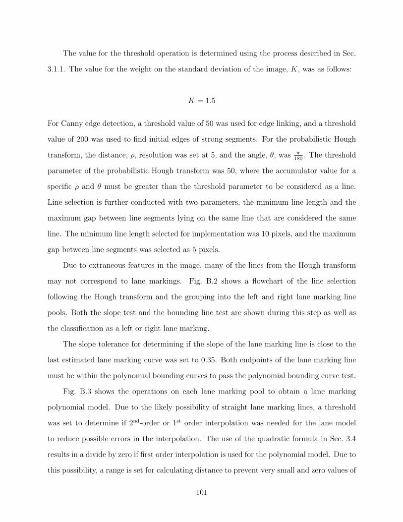
The value for the threshold operation is determined using the process described in Sec.

3.1.1. The value for the weight on the standard deviation of the image, K, was as follows:

K = 1.5

For Canny edge detection, a threshold value of 50 was used for edge linking, and a threshold

value of 200 was used to find initial edges of strong segments. For the probabilistic Hough

transform, the distance, ρ, resolution was set at 5, and the angle, θ, was π180

. The threshold

parameter of the probabilistic Hough transform was 50, where the accumulator value for a

specific ρ and θ must be greater than the threshold parameter to be considered as a line.

Line selection is further conducted with two parameters, the minimum line length and the

maximum gap between line segments lying on the same line that are considered the same

line. The minimum line length selected for implementation was 10 pixels, and the maximum

gap between line segments was selected as 5 pixels.

Due to extraneous features in the image, many of the lines from the Hough transform

may not correspond to lane markings. Fig. B.2 shows a flowchart of the line selection

following the Hough transform and the grouping into the left and right lane marking line

pools. Both the slope test and the bounding line test are shown during this step as well as

the classification as a left or right lane marking.

The slope tolerance for determining if the slope of the lane marking line is close to the

last estimated lane marking curve was set to 0.35. Both endpoints of the lane marking line

must be within the polynomial bounding curves to pass the polynomial bounding curve test.

Fig. B.3 shows the operations on each lane marking pool to obtain a lane marking

polynomial model. Due to the likely possibility of straight lane marking lines, a threshold

was set to determine if 2nd-order or 1st order interpolation was needed for the lane model

to reduce possible errors in the interpolation. The use of the quadratic formula in Sec. 3.4

results in a divide by zero if first order interpolation is used for the polynomial model. Due to

this possibility, a range is set for calculating distance to prevent very small and zero values of

101

Hough lines

Slope Positive?

slope within toleranceof slope of estimated left

lane marking?

both endpoints between left bounding lines?

slope within toleranceof slope of estimated right lane marking?

both endpoints between right bounding lines?

yes

add to left laneline pool

add to right laneline pool

set left lane found flag

set right lanefound flag

no

no

no

yes

yesyes

yes

no

no

Figure B.2: Hough Line Selection

a from causing errors due to divide by zero and overflow conditions of the computer. Within

the range, Eq. (B.1) is used to calculate the distance to the lane marking.

d =y − cb

(B.1)

where d is the distance, y is the row in the image, b is the x coefficient of the polynomial,

and c is the vertical axis intercept. This range is currently set at (−.00001, .00001). The

second diamond block of Fig. B.3 describes how the distance to the lane marking is used

to determine if the estimated lane polynomial is a reasonable estimation for the location

of a lane marking. Since the estimated lane markings should measure a distance that is

reasonable for location within a lane, any estimate of distance within the lane that is far

beyond the lane width and visual angle of the vehicle can be assumed to be a bad estimate.

102

Check threshold of pool size for second order

interpolation

Left or right lanemarking pool

Is the distance calculationof lane model withinreasonable limits?

Accept lane coefficientsCalculate distance

Calculate yawMeasurement update

below

First OrderInterpolation

above

Second OrderInterpolation

a, b, c

yes no

Reject lane coefficients

Figure B.3: Line Processing

Generally this scenario occurs when the system tracks a long white object in the image that

appears like a lane marking but moves to a more horizontal appearance in the image.

The measurement update in the Kalman filter requires all six states of both coefficients

to be measured in order for the system to be observable. However, the left or right lane

markings may not be detected by the vision system and no measurement is made. To

counter this, the H matrix is defined as

H =

1 0 0 0 0 0

0 1 0 0 0 0

0 0 1 0 0 0

(B.2)

when only the right lane marking is detected,

103

H =

0 0 0 1 0 0

0 0 0 0 1 0

0 0 0 0 0 1

(B.3)

when only the left lane marking is detected, and

H =

1 0 0 0 0 0

0 1 0 0 0 0

0 0 1 0 0 0

0 0 0 1 0 0

0 0 0 0 1 0

0 0 0 0 0 1

(B.4)

when both lane markings are detected. The measurement update, then, only changes the

states when a measurement is made. Additionally, since no dynamics are present in the

system, the time update only serves to modify the P matrix. The states, then, only change

when a lane is detected by the vision system.

With two lane markings, the lane with which to choose the distance and yaw must be

chosen. Generally three scenarios are present for lane marking structure within an image.

• dashed left lane marking, solid right lane marking

• dashed right lane marking, solid left lane marking

• both dashed lane markings

For all situations, the solid lane marking is the more easily tracked lane marking and will give

the better estimate of lane marking position and vehicle yaw within the image. Dashed lane

markings can give intermittent measurements of lane position or yaw, but these estimates

can be bad due to bad interpolation from parts of the dashed lane marking. On lane changes

and changes in road structure, the valid lane marking can switch between the left and right

104

lane markings. The determination for distance and yaw, then, should use the lane marking

with the most consistent lane marking from frame to frame. Since the distance measurement

is the distance in the lane with respect to the right lane marking, the typical width of the

lane can be used to determine the lateral distance when only the left marking is found. For

yaw, the intersection of two parallel lines (the lane marking measurements) should be the

location of the horizon line in the image. With just one lane, the typical location of the

horizon can be used instead. The intersection of the lane marking measurement and the

typical location of the horizon can be used to determine yaw. Ideally, both lane markings

would be tracked well and the distance and yaw measurements can be determined from both.

However, rarely are both lane markings solid.

B.2 Vision/IMU Fusion

The vision/IMU system is simulated using real data from an IMU, gps, and vision

measurements. Implementation of the vision / IMU sensor fusion expands the states in the

vision-only Kalman filter to include the states for the IMU, as described in Sec. 4.2. The

measurements of lateral distance and yaw are used for updating the lateral distance and yaw

states in the measurement update. Along with these two measurements are the six states

for the coefficients as used in the Kalman filter for the vision-only system. The data from

GPS, the camera timestamp, and the IMU are read from data files into the system. When

the IMU has the most recent timestamp, the time update for the extended Kalman filter is

called followed by the time update for the vision only system to shift the polynomials based

on the inertial data. When the camera has the most recent timestamp, the vision processing

is conducted, and a measurement update is called using the yaw and lateral distance of the

camera as well as the longitudinal velocity from the most recent gps data. An alternate

strategy is to process the GPS measurements separately from the camera measurements in

different measurement updates, but without a longitudinal velocity measurement from gps,

the system is unobservable.

105

Vision Processing

GPSMeasurement Update

Logged Data

Cameraor

IMUTime Update camera IMU

model coefficientslateral distance

yaw

longitudinalvelocity

longitudinal accelerationyaw rate

Figure B.4: IMU/Camera Integration

Much of the additional code developed for this project was for aiding the research process,

such as creating processed video, histograms, and writing data to text files for later plotting.

106

Appendix C

Alternate EKF Structure

C.1 Closely-Coupled EKF

The structure of the extended Kalman filter is an expansion on the linear filter presented

in Sec. 3.6. The states of the left and right lane models, aL, bL, cL, aR, bR, and cR, make up the

first six states of the filter. Lateral position py, which is updated through the measurement

of distance from the images, and lateral velocity vy are the next two states. The lateral

acceleration bias, bay, and yaw, ψ, make up the final two states of the filter.

x =

[aL bL cL aR bR cR py vlong blong ψ bψ

]T(C.1)

The difference in performance between the closely coupled and loosely coupled versions of

the filter is small. As seen in Fig. C.1, the most significant difference between the closely

coupled filter and the results seen for the loosely coupled filter in Fig. 4.9 is during the first

lane marking outage, where the estimate does not drift significantly compared with the drift

of the loosely coupled algorithm. While this appears significantly better than the loosely

coupled version, more likely the filter is merely better tuned for that particular segment of

the run in the closely coupled filter, and the bias is better estimated.

Fig. C.2 shows the closely coupled heading estimate compared with truth. Again, the

results are very similar to the loosely coupled version.

One significant difference, however, is the computation time for inverting the matrix

needed in the calculation for the gain in the measurement update, shown in Eq. (C.2).


T +R)−1 (C.2)

107

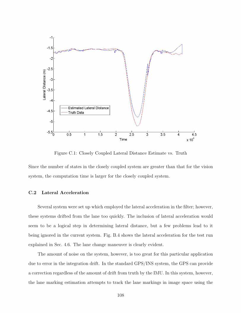
Figure C.1: Closely Coupled Lateral Distance Estimate vs. Truth

Since the number of states in the closely coupled system are greater than that for the vision

system, the computation time is larger for the closely coupled system.

C.2 Lateral Acceleration

Several system were set up which employed the lateral acceleration in the filter; however,

these systems drifted from the lane too quickly. The inclusion of lateral acceleration would

seem to be a logical step in determining lateral distance, but a few problems lead to it

being ignored in the current system. Fig. B.4 shows the lateral acceleration for the test run

explained in Sec. 4.6. The lane change maneuver is clearly evident.

The amount of noise on the system, however, is too great for this particular application

due to error in the integration drift. In the standard GPS/INS system, the GPS can provide

a correction regardless of the amount of drift from truth by the IMU. In this system, however,

the lane marking estimation attempts to track the lane markings in image space using the

108

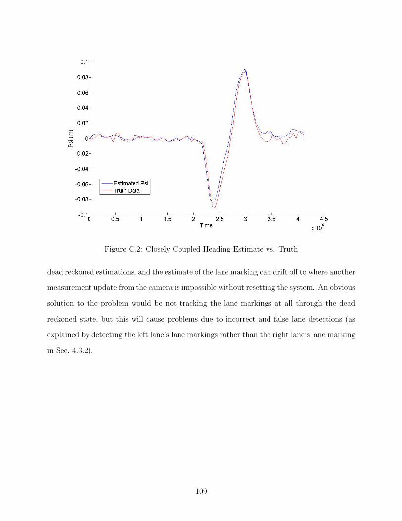
Figure C.2: Closely Coupled Heading Estimate vs. Truth

dead reckoned estimations, and the estimate of the lane marking can drift off to where another

measurement update from the camera is impossible without resetting the system. An obvious

solution to the problem would be not tracking the lane markings at all through the dead

reckoned state, but this will cause problems due to incorrect and false lane detections (as

explained by detecting the left lane’s lane markings rather than the right lane’s lane marking

in Sec. 4.3.2).

109

Figure C.3: Lateral Acceleration

110

Lane Level Localization with Camera and Inertial ...

Documents

Transcript of Lane Level Localization with Camera and Inertial ...