Landscape, vegetation characteristics, and group identityin an urban and suburban watershed: why the 60s matter

Christopher G. Boone & Mary L. Cadenasso &

J. Morgan Grove & Kirsten Schwarz &

Geoffrey L. Buckley

Published online: 20 November 2009# The Author(s) 2009. This article is published with open access at Springerlink.com

Abstract As highly managed ecosystems, urban areas should reflect the social character-istics of their managers, who are primarily residents. Since landscape features develop overtime, we hypothesize that present-day vegetation should also reflect social characteristics ofpast residents. Using an urban-to-suburban watershed in the Baltimore MetropolitanRegion, this paper examines the relationship between demographics, housing character-istics, and lifestyle clusters from 1960 and 2000 with areas of high woody and herbaceousvegetation cover in 1999. We find that 1960 demographics and age of housing are betterpredictors of high woody or tree coverage in 1999 than demographics and housingcharacteristics from 2000. Key variables from 1960 are percent in professional occupations(+), percent of pre-WWI housing (−), percent of post-WWII housing (+), and populationdensity (−). Past and present demographic and housing variables are poor predictors of highherbaceous cover in 1999. Lifestyle clusters for 2000 are very good predictors of highherbaceous coverage in 1999, but lifestyle clusters from 1960 and 2000 are poor predictorsof high woody vegetation coverage. These findings suggest that herbaceous or grassy areas,typically lawns, are good reflections of contemporary lifestyle characteristics of residentswhile neighborhoods with heavy tree canopies have largely inherited the preferredlandscapes of past residents and communities. Biological growth time scales of trees and

Urban Ecosyst (2010) 13:255–271DOI 10.1007/s11252-009-0118-7

C. G. Boone (*)School of Human Evolution & Social Change, School of Sustainability, Arizona State University, P.O.Box 875502, Tempe, AZ 85287-5502, USAe-mail: cgboone@asu.edu

M. L. CadenassoDepartment of Plant Sciences, University of California-Davis, Davis, CA, USA

J. M. GroveNorthern Research Station, USDA Forest Service, Baltimore, MD, USA

K. SchwarzEcology and Evolution, Rutgers University, New Brunswick, NJ, USA

G. L. BuckleyDepartment of Geography, Ohio University, Athens, OH, USA

woody vegetation means that such vegetation may outlast the original inhabitants whodesigned, purchased, and planted them. The landscapes we see today are therefore legaciesof past consumption patterns.

Keywords Urban landscapes . Social predictors . Legacies . Baltimore

Introduction

Urban ecosystems are highly managed in order to meet primarily the needs and wishes ofpeople (Dow 2000; Grimm et al. 2008). As such, the vegetation landcover in cities typicallyreflects, in addition to the biophysical potential and limitations of the site, the culture andvalues of people and decision makers who plant and care for trees, shrubs, gardens, andgrass (Spirn 1984; Burgi et al. 2004). Vegetation in cities can serve fundamental purposesof providing food (fruits and vegetables), shade, or play and recreation areas. Economistshave also demonstrated that lush and well maintained trees and yards can add value tohomes (Luttik 2000; Mansfield et al. 2005).

Landscaping and gardening can help build connections with “nature,” serve as hobbies,and satisfy a yearning for beauty. They can also convey status or serve as external markersof who lives inside the dwelling beyond the front yard. Some research, described below,also shows that landscaping reflects more than individual character. Even on privateproperty, the choice of landscaping may mirror the vegetation patterns of surroundingproperties and the neighborhood as a whole. Pressure to conform and the status associatedwith a well-kept yard, which Troy et al. (2007) term an “ecology of prestige,” can result inneighborhoods swathed in similar green lawns and trees. Landscaping firms also fuel thedesire to keep up with the neighbors (Robbins 2007). Even when residents who callthemselves environmentalists and understand the negative ecological consequences offertilizing lawns, the pressure is great enough that they will do so regardless.

Urban landscapes typically have very little productive value in terms of economicreturns to consumers; rather they are more often forms of consumption. Similar to othertypes of consumption, landscapes should reflect the status and characteristics of theconsumer at both the individual or household level as well as the neighborhood. However,landscapes, especially woody vegetation, are not instant—they depend on biological growthtime scales that may outlast the original inhabitants who designed, purchased, and plantedthem. The landscapes we see today are therefore legacies of past consumption patterns. Thispaper addresses the question of whether socio-demographic and housing characteristics ofthe past are significant predictors of urban landcover of the present, using the Gwynns FallsWatershed in Metropolitan Baltimore as a case study.

Social predictors of urban landscapes

Urban landscapes are heterogeneous, a patchwork of built and vegetation land covers,multiple land uses, and social groupings. Because urban landscapes are highly managed, itfollows that the patchwork of cities should reflect the characteristics, preferences, resources,efforts, and influences of their managers, including homeowners. Existing research showsthat the distribution of trees and grassy lawns in cities are, like most urban characteristics,uneven, and that those patterns are related to social characteristics of neighborhoods.

As one would expect, scarcity of tree and grass cover is typically a function ofpopulation density. As population densities increase, vegetation cover tends to decline as

256 Urban Ecosyst (2010) 13:255–271

built-residential uses out-compete non-built land uses (Nowak et al. 1996; Iverson andCook 2000). However, population density alone cannot explain the variation in vegetationcover in cities. Suburbs usually contain more green cover than downtown cores, but withinurban areas, the leafiest and greenest areas are often also the wealthiest (Talarchek 1990;Martin et al. 2004; Jensen et al. 2004; Mennis 2006). This association between wealth andvegetation has been observed for cities in the United States and elsewhere (Escobedo et al.2006; Kirkpatrick et al. 2007; Conway and Hackworth 2007). These findings suggest thatgreater wealth provides residents and neighborhoods with more resources to plant and takecare of vegetation, and the greenness of wealthy communities may be self-reinforcing, as itattracts more wealthy residents. Trees and green spaces also increase property values, whichincreases tax bases for planning and maintenance of public spaces, and may attract furtherhigh-income buyers to the neighborhood.

Although income is an important predictor of vegetation, other social characteristicssuch as education and ethnicity are strongly associated with greenspace in cities. A study ofurban forest canopy cover in 60 cities in central Indiana, for instance, found that tree coverwas significantly and positively correlated with percent of persons holding a college degree(Heynen and Lindsey 2003). Landscapes also reflect dominant cultures. In a study ofvegetation characteristics and ethnicity in Toronto, homeowners of British heritage weremore likely to have shade trees on their properties than persons of Chinese ancestry (Fraserand Kenney 2000).

Others have pointed to lifestyles, typologies of neighborhoods or individuals based on acombination of socioeconomic and housing characteristics, as key determinants ofvegetation. In a study of vegetation on private property parcels in Baltimore, Troy et al.(2007) found that lifestyle categories were strongly correlated with what they term realizedstewardship, or the percent of potential pervious surface on properties that is vegetated.Specifically they found that a well-educated but less wealthy lifestyle category has 52% lessrealized stewardship than the well-educated and higher income lifestyle group. Even thoughthe population densities are similar, the first lifestyle group tends to be younger and morelikely to live in rental or multi-unit housing than the second lifestyle group. Other studieshave found that renters live in areas with lower urban tree canopy cover than homeowners(Emmanuel 1997; Perkins et al. 2004). Renter is a social class and a housing characteristic,both of which tend to result in less commitment to long term property maintenance, short-term or temporary timelines for residents, and relatively weak political power to demandcity services, such as street trees.

Vegetation characteristics of properties are also the result of a neighborhood effect.Property owners often mimic the landscaping practices and preferences of theirneighbors (Zmyslony and Gagnon 2000). Grove et al. (2006) describe this phenomenonof mimicry as an ecology of prestige, the phenomenon in which household patterns ofconsumption and expenditure on environmentally relevant goods and services aremotivated by group identity and perceptions of social status associated with differentlifestyles (Grove et al. 2005; Law et al. 2004). This theory suggests that a household’sland management decisions are influenced by the desire to uphold the prestige of itscommunity and outwardly express its membership in a given lifestyle group. Conceptionsof luxury and prestige, however, are highly variable, even within the same income ordemographic group. Lifestyle variables may only be weakly correlated with socio-economic status, such as family size, marriage status, and life stage. However, lifestylecan play a critical role in determining where households choose to locate and how theymanage their properties (Timms 1971; Knox 1994; Short 1996; Gottdiener andHutchinson 2000; Kaplan et al. 2004).

Urban Ecosyst (2010) 13:255–271 257

Legacy effects on urban landscapes

In newly-built suburbs, the vegetation cover may be an expression of the current social andhousing characteristics of the resident or neighborhood, although it is more likely theperception of what the developer believes will satisfy buyers. Newly-built neighborhoodsare also more likely to have new vegetation, such as small saplings, especially if the landwas formerly agricultural or the developer clears forests for construction. In longestablished neighborhoods, where residents have come and gone, existing vegetation mayreflect the tastes and wishes of past residents. People moving into older homes thus inheritpast social preferences of landscapes. Even in newly-built suburbs, legacies from past landuses, such as woodlands or agricultural fields, may put their stamp on current landscapes(Dow 2000). A central question of this research is whether past social and housingcharacteristics are better predictors of woody and herbaceous vegetation than current socialand housing characteristics. Some prior research, though limited, suggests that pastinhabitants and age of housing are significant predictors of current vegetation in urban areas(Heynen and Lindsey 2003; Martin et al. 2004). In a pioneering study, Grove (1996) foundthat 1970 social characteristics were the best predictors of 1990 vegetation in the GwynnsFalls Watershed of Baltimore. Using a parcel-level analysis, age of housing was also foundto be an important predictor of vegetation abundance in Baltimore City (Grove et al. 2006;Troy et al. 2007). Amount of realized stewardship, or percent cover of potentially vegetatedsurface per parcel, shows an inverted-U relationship with age of housing, peaking in 1950(Troy et al. 2007). This article builds on Grove’s (1996) analysis of the Gwynns FallsWatershed by using an updated and high resolution land cover layer of vegetation, censusdata from 2000, and by examining, in addition to demographics and housing, theassociation between lifestyle and vegetation cover. Group identity, we argue, is a powerfulforce in defining neighborhood characteristics, including its vegetation.

Group identity

Group identity can be expressed in a number of material ways, from gang colors, touniforms, to flags. It can also be manifest in the landscape, as generations of socialscientists have shown (Sauer 1925; Cosgrove 1998). The study of the cultural landscape iswell established, albeit with a bias toward the rural rather than urban. A trained scholar canpick out remnants of past cultures, even from very fragmentary evidence; the shape of abarn, the construction of a fence, or shards of pottery are used to identify folkways that bindtogether individuals into groups through a common way of doing something (Anderson2001). When studying the urban environment, making the linkage between the legacies ofculture, or group identity, and landscape can tell us more about the dynamics of urbanecology compared to purely contemporary associations (Dow 2000; Cadenasso et al. 2006).In this paper we argue that group dynamics are key to understanding behavior that impactslandscape management at the neighborhood level.

Identifying what constitutes a group is a difficult endeavor, something that has keptlegions of social scientists busy for decades (Côté and Levine 2002). Single variables likerace, income, or education can go a long way in teasing apart the elements of groupidentity, but given their colinearity, a number of methods have been derived to search forthe bundle of variables that tell us what makes groups different and separate from oneanother. Part of group identity is defined by where people live (Weiss 2000). Similarindividuals or households cluster geographically. These clusters may be self-reinforcing byattracting similar people to certain neighborhoods, strengthening a sense of neighborhood

258 Urban Ecosyst (2010) 13:255–271

or group identity, and at the same time shunning those that do not share that group’s identity(Massey and Denton 1993). Cities are, however, dynamic places and such patterns can shiftover time. Every reader can think of a neighborhood that has changed in socialcharacteristics, sometimes slowly and sometimes surprisingly quickly. On the other hand,many neighborhoods and the characteristics of people who inhabit them can remainremarkably stable. In neighborhoods there is a high amount of fixed, social, and evenemotional capital, sometimes referred to as attachment to place. Such investments will becarefully guarded and defended, in extreme cases through violence and intimidation. Insubtler ways neighborhoods retain their identity because the sense of group membership isso strong that few outsiders feel welcome. As disagreeable as clustering (or put anotherway, segregation) may seem to some, it is a powerful force that shapes patterns andprocesses of urban landscapes.

Methods

Lifestyle clusters

Marketers are wise to the linkages between consumption patterns and group identity asexpressed through shared traits, including location. They have found that targetedmarketing for many products is more efficient and effective than a shotgun approach.Given the very real value of this information, companies have seized on the opportunity toprovide such information to vendors. In 1976, the Claritas Corporation (now owned by theNielson Company) developed the PRIZM* (Potential Rating Index for Zip Codes) marketsegmentations and sells this product as a marketing tool. The segmentation uses factor andcluster analyses of census data, and releases its results using census geographic units—thecensus block group, census tract—and at the zip code level. Point of purchase data is thenmatched to the lifetsyle clusters, so that the company can tell vendors what types ofproducts are likely to sell well in particular zip codes or census tracts. For this study, we usePRIZM lifestyle classifications at the census tract level for 2000 and generate pseudo-PRIZM lifestyle clusters for 1960, described below. These data are overlaid onto avegetation layer derived from 1999 orthoimagery.

Land cover classification

To overcome limitations of using the Anderson land classification system in urban areas,we use a new classification developed by Cadenasso et al. (2007) that describes biophysicalheterogeneity of urban landscapes at fine scales. This classification is called HERCULES(High Ecological Resolution Classification for Urban Landscapes and EnvironmentalSystems) and is built using a logic of land cover. HERCULES describes variation in threeurban physical elements—buildings, vegetation, and surfaces (Ridd 1995). Within thesethree elements, variation in the building type and cover, vegetation type and cover, and typeand cover of surfaces, determines a patch boundary and classification.

To create a HERCULES patch layer, high resolution digital aerial imagery was used.The imagery was collected for the Gwynns Falls watershed in October 1999. It is threeband color infrared, with green (510–600 nm), red (600–700 nm), and near infrared (800–900 nm) bands. Pixel size for the imagery is 0.6 m. Land cover patches, using theHERCULES system, were digitized and the proportion cover of each component estimatedvia visual interpretation. The patch layer can be queried for variation in any one feature or

Urban Ecosyst (2010) 13:255–271 259

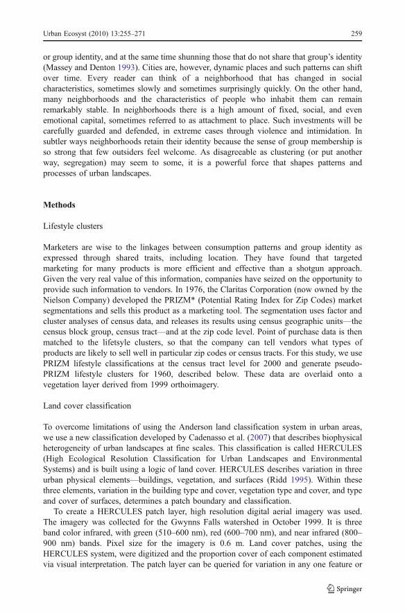
combination of two or more features. In the analysis presented here, patches that containedgreater than 75% cover of woody vegetation or fine vegetation were used (Fig. 1). Wechose only these categories in order to examine associations between population andhousing characteristics and patches with a high percentage of woody (coarse) vegetationand a high percentage of herbaceous (fine) vegetation cover.

0 2 41 Kilometers

0 20 4010 km

>75% fine vegetation

>75% coarse vegetation

Baltimore City

Baltimore County

Howard County

Middle Bran

Baltimore

Washington, DC

Pennsylvania

Maryland

Virginia

WV

DE

Fig. 1 Patches that contain greater than 75% coverage of coarse woody vegetation and fine herbaceousvegetation according to HERCULES classification for the Gwynns Falls watershed, 1999

260 Urban Ecosyst (2010) 13:255–271

Lifestyle clusters, 1960

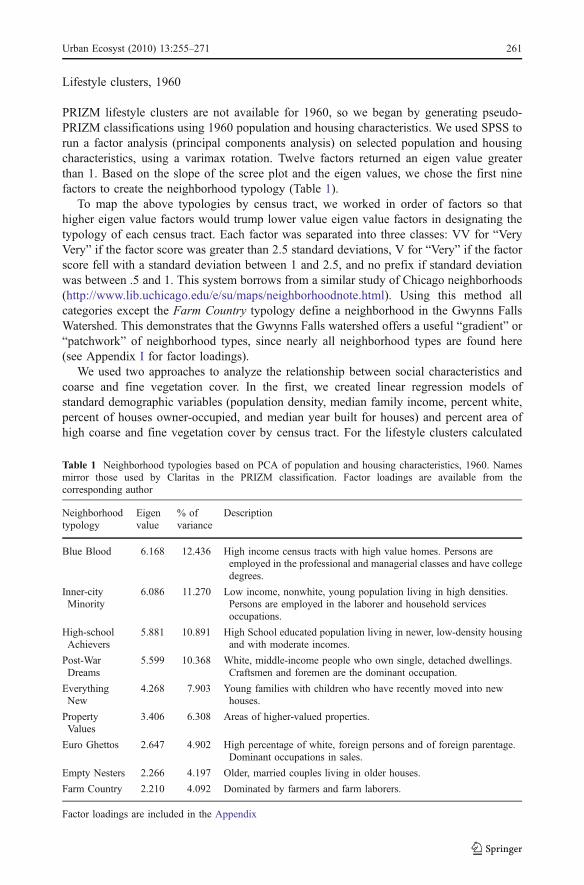
PRIZM lifestyle clusters are not available for 1960, so we began by generating pseudo-PRIZM classifications using 1960 population and housing characteristics. We used SPSS torun a factor analysis (principal components analysis) on selected population and housingcharacteristics, using a varimax rotation. Twelve factors returned an eigen value greaterthan 1. Based on the slope of the scree plot and the eigen values, we chose the first ninefactors to create the neighborhood typology (Table 1).

To map the above typologies by census tract, we worked in order of factors so thathigher eigen value factors would trump lower value eigen value factors in designating thetypology of each census tract. Each factor was separated into three classes: VV for “VeryVery” if the factor score was greater than 2.5 standard deviations, V for “Very” if the factorscore fell with a standard deviation between 1 and 2.5, and no prefix if standard deviationwas between .5 and 1. This system borrows from a similar study of Chicago neighborhoods(http://www.lib.uchicago.edu/e/su/maps/neighborhoodnote.html). Using this method allcategories except the Farm Country typology define a neighborhood in the Gwynns FallsWatershed. This demonstrates that the Gwynns Falls watershed offers a useful “gradient” or“patchwork” of neighborhood types, since nearly all neighborhood types are found here(see Appendix I for factor loadings).

We used two approaches to analyze the relationship between social characteristics andcoarse and fine vegetation cover. In the first, we created linear regression models ofstandard demographic variables (population density, median family income, percent white,percent of houses owner-occupied, and median year built for houses) and percent area ofhigh coarse and fine vegetation cover by census tract. For the lifestyle clusters calculated

Table 1 Neighborhood typologies based on PCA of population and housing characteristics, 1960. Namesmirror those used by Claritas in the PRIZM classification. Factor loadings are available from thecorresponding author

Neighborhoodtypology

Eigenvalue

% ofvariance

Description

Blue Blood 6.168 12.436 High income census tracts with high value homes. Persons areemployed in the professional and managerial classes and have collegedegrees.

Inner-cityMinority

6.086 11.270 Low income, nonwhite, young population living in high densities.Persons are employed in the laborer and household servicesoccupations.

High-schoolAchievers

5.881 10.891 High School educated population living in newer, low-density housingand with moderate incomes.

Post-WarDreams

5.599 10.368 White, middle-income people who own single, detached dwellings.Craftsmen and foremen are the dominant occupation.

EverythingNew

4.268 7.903 Young families with children who have recently moved into newhouses.

PropertyValues

3.406 6.308 Areas of higher-valued properties.

Euro Ghettos 2.647 4.902 High percentage of white, foreign persons and of foreign parentage.Dominant occupations in sales.

Empty Nesters 2.266 4.197 Older, married couples living in older houses.

Farm Country 2.210 4.092 Dominated by farmers and farm laborers.

Factor loadings are included in the Appendix

Urban Ecosyst (2010) 13:255–271 261

for 1960 and the PRIZM classes for 2000, since they are categorical, we created dummyvariables and regressed them against the percent coverage of census tracts for high and lowcoarse vegetation and for high fine vegetation (for 1999).

Results

Legacy effects: Population and housing characteristics

The first set of analyses test the relationships between population and housing character-istics and coarse vegetation cover. We find that past social and housing characteristics arebetter than present social and housing characteristics for predicting current coarsevegetation cover in the Gwynns Falls Watershed. Using the 1960 census tract data,bivariate analyses show a positive and significant relationship between percent of area withhigh coarse vegetation cover from 1999 and (i) percent in professional occupations; and (ii)percent houses built between 1950 and 60. The relationship is negative and significant for(iii) percent houses built before 1940; (iv) population density; and (v) percent nonwhite.Using 2000 census data, only median family income (+) and population density (−) aresignificantly correlated with percent coverage of high coarse vegetation (Table 2).

Using linear regression, we find that the best model for predicting the percent coverageof high coarse vegetation in 1999 are variables from the 1960 census, including percent inprofessional occupations (+) and percent of houses built before 1940 (−). This model has anadjusted R2 of .342, with a standardized beta coefficient of .306 (sig. .018) for percentprofessional, and −.347 (.008 significance) for percent of housing built before 1940. Thebest model using 2000 census data returned an adjusted R2 of .222, with a standardized betacoefficient of −.405 (sig. .000) for population density, and .112 (.045 significance) formedian family income.

Troy et al. (2007) have shown an inverted-U relationship between age of housing and“realized stewardship” at the parcel level. Simply put, the amount of coarse canopy cover islow on properties of older houses, highest for houses built around 1950, and lower fornewer houses. For newer homes, this in part may be a function of growing periods of trees,but may also be a function of changing lifestyle choices, from one of small houses on largelots to large houses on smaller lots. Older neighborhoods, built before the widespread use ofthe automobile, also tend to have higher densities, reducing the opportunities for extensivetree canopies. In Baltimore, this is typified by the iconic row houses that face directly on

Table 2 Correlation coefficients (Spearman’s rho) for 1960 and 2000 census data and percent of high coarsevegetation cover in 1999 by census tract

Independent variables % CT coverage of high coarse vegetation class (1999)

% professional occupations (1960) .542**

% houses built 1950–60 (1960) .510**

% houses built before 1940 (1960) −.556**Population density (1960) −.510**% nonwhite (1960) −.372**Median family income (2000) .334**

Population density (2000) −.466**

**significant at the p<.0001 level

262 Urban Ecosyst (2010) 13:255–271

the street with little or no setback from the sidewalk. Planting trees under these conditionsis difficult and costly, and increases morbidity and mortality rates of trees (Nowak et al.2004). Street tree planting can be more than a technical challenge; in some neighborhoodstrees are seen as a nuisance (Buckley 2010).

We find in this study that the age of housing 40 years ago continues to affect coarsevegetation cover today. In census tracts that had a greater percentage of newer housing(built between 1950 and 1960), the percentage of present-day coarse vegetation cover tendsto be larger than for census tracts that had older housing (built before 1940). This could be afactor of tree death and households not replanting, or it could be that trees were not plantedto the same degree in older neighborhoods as in newer communities.

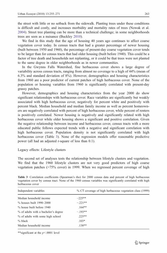
In the Gwynns Falls Watershed, fine herbaceous cover shows a large degree ofvariability across census tracts, ranging from almost no coverage to a high of 44% (mean of6.3% and standard deviation of 8%). However, demographics and housing characteristicsfrom 1960 are a poor predictor of current patches of high herbaceous cover. None of thepopulation or housing variables from 1960 is significantly correlated with present-daygrassy patches.

However, demographics and housing characteristics from the year 2000 do showsignificant relationships with herbaceous cover. Race variables are significantly but weaklyassociated with high herbaceous cover, negatively for percent white and positively withpercent black. Median household and median family income as well as percent homeown-ers are negatively correlated with percent of high herbaceous cover, while percent of rentersis positively correlated. Newer housing is negatively and significantly related with highherbaceous cover while older housing shows a significant and positive correlation. Giventhe negative relationship between income and herbaceous cover, census tracts with a moreeducated public follows expected trends with a negative and significant correlation withhigh herbaceous cover. Population density is not significantly correlated with highherbaceous cover (Table 3). None of the regression models offer reasonable predictivepower (all had an adjusted r-square of less than 0.1).

Legacy effects: Lifestyle clusters

The second set of analyses tests the relationship between lifestyle clusters and vegetation.We find that the 1960 lifestyle clusters are not very good predictors of high coarsevegetation patches (>75% cover) in 1999. When we regressed percent coverage of high

Table 3 Correlation coefficients (Spearman’s rho) for 2000 census data and percent of high herbaceousvegetation cover by census tract. None of the 1960 census variables was significantly correlated with highherbaceous cover

Independent variables % CT coverage of high herbaceous vegetation class (1999)

Median household income −225**% houses built 1990–2000 −.221**% house built before 1940 .164**

% of adults with a bachelor’s degree −.193**% of adults with some high school .225**

% black .103*

Median household income .138**

**significant at the p<.0001 level

Urban Ecosyst (2010) 13:255–271 263

coarse vegetation against dummy variables for neighborhood typology, the model returnedan adjusted R2 of only .057. Descriptive statistics show that, of the neighborhoods thatcontain high coarse vegetation patches, Post-War Dreams had the highest mean value(15.9%) of coverage, followed by the Very High School Achievers (14.1%) and High SchoolAchiever (13.5%) neighborhoods. The lifestyle clusters were better, however, at predictingthe lack of coarse vegetation patches. The model returned an adjusted R2 of .234 (sig. .000).But only two (Property Values and Very Inner-City Minority) of the twelve dummyvariables were significant. The descriptive statistics show that High School Achievers(28.3%) and Very High School Achievers (19.6%) had the highest mean percentage of lowcoarse vegetation coverage, followed by Property Values (19.6%). Lack of coarsevegetation does not, of course, equate with lack of vegetation. These three neighborhoodtypes also contain the highest mean percentage of fine vegetation (mainly grass).

The 2000 lifestyle clusters from PRIZM are also not very good predictors of highcoarse or woody vegetation coverage. The model returned an adjusted R2 of .041. Of the31 PRIZM classes that contained a patch of high coarse vegetation cover, Mid-City Mixhad the highest mean percentage (23.6%), followed by Inner Cities (22.9%) and Upstarts& Seniors (10.9%). Similar to the 1960 lifestyle clusters, PRIZM classifications are betterat predicting a lack of coarse vegetation patches. This model generated an adjusted R2 of.297 (sig. .000). PRIZM classes with the highest mean values of low coarse vegetationcoverage are Executive Suites (19.6%), Kids and Cul-de-Sacs (13.8%), and NewBeginnings (12.1%).

PRIZM classes are, however, much better at predicting high fine vegetation coverage(grass and herbaceous cover). The model generates an adjusted R2 of .361 (sig .000).Descriptive statistics show that the highest mean values are for Mid-City Mix (25.5%), NewEmpty Nests (21.7%), and Suburban Sprawl (10.4%). Lifestyle clusters for 1960 are not asstrong in predicting present-day coverage of fine vegetation. That model returned anadjusted R2 of .150 (sig. 000), better than for the coarse vegetation model but weaker thanthe PRIZM classes model.

Discussion

When it comes to understanding present tree canopy patterns in the Gwynns FallsWatershed, the 1960s matter. Using population and housing characteristics, we find thatneighborhoods that had a high percentage of professionals and a low percentage of pre-WWII houses in 1960 are now the leafiest neighborhoods in the watershed. Neighborhoodsthat have high median incomes and low population densities in 2000 are also goodpredictors of high coarse vegetation, but the 1960 characteristics are more significant.

Lifestyle clusters in 1960 are not very good at predicting the amount of coarsevegetation in 2000, but are better at predicting the lack of it. The same holds true for thePRIZM classes for the year 2000. However, PRIZM classifications are very good predictorsof fine vegetation coverage (e.g. grass and fine herbaceous cover). 1960 lifestyle clustersare better at predicting fine vegetation than coarse vegetation coverage, but are not as strongas PRIZM classes. Neither the 1960 nor the 2000 demographics are good predictors of highfine vegetation coverage. In summary, 1960 demographics are better predictors of high treecover, while current lifestyle classes are better predictors of high grass cover in the GwynnsFalls Watershed (Table 4). These results suggest that lawns are better connected to lifestylethan trees, while demographics and housing, especially those from decades ago, are betterpredictors of trees than grass.

264 Urban Ecosyst (2010) 13:255–271

The association between demographics, lifestyle clusters, and vegetation patterns issimply that—an association—but it points to social and housing characteristics that shouldbe investigated further. Those in professional occupations in 1960 may have been theindividuals who planted and cared for trees, or it could be that professionals were attractedto already leafy districts of the city. Since part of the canopy cover is in parks, it is possiblethat professionals were attracted to neighborhoods close to parks, or lobbied for theirmaintenance and care. An analysis of historic landcover patterns may provide clues.

The social and housing legacies on the landscape must also be placed in their appropriatecontexts (Conway and Urbani 2007). Timing of growth is important not only for permittingbiological growth and senescence of trees or other vegetation, but also corresponds withparticular cultural and legal milieus. Post-WWII housing differed markedly from pre-warhousing, with a greater emphasis on detached single family homes for a growing middleclass, fueled by federal mortgage subsidies and federally funded highways (Hayden 2003).The detached home set in a landscaped garden was not unique to this era, but the scale ofdevelopment was significantly greater in the 1950s than the 1930s. New building codes thatrequired minimum set-backs from streets, and zoning laws that forbade mixed-usedevelopment helped to move Baltimore housing away from its iconic row houseneighborhoods to neighborhoods of houses in a sea of green grass.

Place histories matter as well. In the well-treed neighborhood of Mount Royal, forinstance, a long history of racial segregation likely contributed to the distribution of treeswe see today. Owing to a neighborhood improvement association that actively promotedtree planting and a restrictive covenant that reserved properties within the area for whiteoccupancy only, a disproportionate share of amenities—in this case trees—flowed intoMount Royal while a host of disamenities such as polluting industries and undesirablecommercial development was redirected elsewhere (Buckley 2010). Larger socio-spatialtrends, such as white and middle-class flight, the tide of suburbanization, and massiveeconomic restructuring from an industrial to a service economy all left their imprint on thesocial and landscape configurations of the watershed.

Linking social characteristics to vegetation patterns has very practical applications. In 2006,the City of Baltimore declared that it would double its tree canopy cover over the next twentyyears. This ambitious goal is one of many efforts across the United States to reestablish treesand parks in cities as natural amenities that provide multiple ecological and social benefits.Baltimore has a long history of street tree planting; it was one of the first cities in the country toestablish a City Forestry Division after passing a Tree Ordinance in 1912. Then as now, themunicipal administration recognized that trees would beautify the city, clean the air, increaseproperty values, regulate extremes of temperature, and reduce loads on stormwater systems.

What may have been forgotten is that trees in the city were not universally loved andadmired. Newspaper accounts from the 1950s and 1960s reveal that some residents,

Table 4 Strength of associations between 1960 and 2000 demographics/housing and lifestyle with patchesof high coarse and high fine vegetation in 1999

Independent variable group High coarse vegetationcover in 1999 (Trees)

High fine vegetationcover in 1999 (Grass)

1960 Demographics/housing Best Poor

Lifestyle Poor Fair

2000 Demographics/housing Good Fair

Lifestyle Poor Best

Urban Ecosyst (2010) 13:255–271 265

especially those living in East Baltimore, were hardly enamored with the idea of havingstreet trees planted in their neighborhoods. As long-time city forester Charles Younglamented in a 1955 interview: “I was under the impression that all people like to have treesplanted in front of their houses until I started planting trees in front of houses” (Evening Sun24 May 1955). Some East Baltimoreans’ disdain for trees was carried to an extreme. “I justdon’t like trees,” confessed one resident in 1967. “I don’t like greenery. I like clean,uncluttered concrete” (Evening Sun 25 April 1967). More recently in New York City, aninitiative to plant one-million trees in the city’s boroughs has prompted pockets ofresistance. Some residents have protested that street trees will worsen their allergies, dropbranches on their cars, or that the roots will penetrate their foundations. A public relationscampaign to ease some of those concerns has not convinced all New Yorkers of the valuesof street trees. That residents are responsible for raking leaves does not help matters(Dominus 2008). These stories suggest that simply planting trees does not mean Baltimoreor New York will achieve its goals. Because households are responsible for much of a city’svegetation, the success of such efforts will depend, in part, on understanding the socialpredictors of vegetation (Yaoqi et al. 2007).

Baltimore’s goal of doubling its tree canopy cannot be carried out without trees beingplanted and cared for on private land in addition to public land (City of BaltimoreRecreation and Parks 2007). Annual tree mortality rates in Baltimore are close to 7%, partlydue to neglect, and new young trees are particularly susceptible (Nowak et al. 2004). Thatbeing the case, it is imperative to know why trees thrive in some communities and not inothers, beyond the physical properties of the sites. Stormwater management, includingreduction of impervious surfaces and protection of the Chesapeake from fertilizer runoff,will be most effective if managers understand relationships between social characteristicsand vegetation cover (Cadenasso et al. 2007; Pickett et al. 2008). Since the vast majority ofland is privately owned, it is the decisions of individuals and households, which oftenreflect characteristics of neighborhoods, that are crucial to understand. As the 1960s matterfor understanding the present distribution of trees in Baltimore, the 2000s will matter forcity managers as they attempt to green the city over the next 40 years.

Acknowledgments Research for this article was supported through awards from the National ScienceFoundation Long-Term Ecological Research program (DEB 0423476), the National Science Foundation Humanand Social Dynamics program (SBE–HSD 0624159), and the U.S. Department of Agriculture Forest Service(06JV11242300039). The authors thank the anonymous reviewers for their insightful comments and suggestions.

Open Access This article is distributed under the terms of the Creative Commons AttributionNoncommercial License which permits any noncommercial use, distribution, and reproduction in anymedium, provided the original author(s) and source are credited.

Appendix I: Factor loadings for PCA of 1960 population and housing characteristicsby census tract

Blue BloodEigen value: 6.168Percent of Variance: 12.436Characteristics: High income census tracts with high value homes. Persons areemployed in the professional and managerial classes and have college degrees.Factor loadings:[.900] percent of families with annual incomes greater than $25,000

266 Urban Ecosyst (2010) 13:255–271

[.879] percent of all housing units with value of more than $35 K[.838] percent of families with annual income less between $15,000 and $25,000[.801] percent of all housing units with value of between $25 and 35 K[.819] percent of persons over 25 years of age with 4 years or more of college education[.608] percent of employed civilians 14 and over, professional, technical, and kindred workers[.429] percent of employed civilians 14 and over, managers, officials, and proprietors

[−.522] percent of persons over 25 years of age with 8 years or less education[−.491] percent of employed civilians 14 and over, operatives and kindred workers,including mine

Inner-city MinorityEigen value: 6.086Percent of Variance: 11.270Characteristics: Low income, nonwhite, young population living in high densities.Persons are employed in the laborer and household services occupations.Factor loadings:[.802] percent of population nonwhite[.801] percent of population between 5 and 19 years[.763] percent of employed civilians 14 and over, private household workers[.750] percent of population under 5 years[.630] percent of employed civilians 14 and over, laborers, except farm and mine[.564] percent of families with annual income less between $1,000 and $5,000[.517] percent of families with annual income less than $1,000[.455] population density, persons per square kilometer

[−.767] percent of population between 20 and 64 years[−.674] percent of population white

High School AchieversEigen value: 5.881Percent of Variance: 10.891Characteristics: High School educated population living in newer, low-densityhousing and with moderate incomes.Factor loadings:[.720] percent of all housing units with value of between $10 and 12.5 K[.688] percent of persons over 25 years of age with 4 years of high school education[.662] percent of houses moved into between 1954 and 1957[.513] percent of all housing units with value of between $12.5 and 15 K[.495] percent of families with annual income less than $1,000[.479] percent of houses built between 1950 and 1960

[−.800] percent of all housing units with value of under $5,000[−.623] percent of all housing units with value of between $5 and 7.5 K[−.553] percent of families with annual income less between $1,000 and $5,000[−.543] percent of families with annual income less than $1,000[−.528] percent of houses built before 1940[−.503] percent of employed civilians 14 and over, laborers, except farm and mine[−.461] population density, persons per square kilometer[−.432] percent of houses moved into before 1940

Urban Ecosyst (2010) 13:255–271 267

Post-War DreamsEigen Value: 5.599Percent of Variance: 10.368Characteristics: White, middle-income populations who own single, detached dwell-ings. Craftsmen and foremen are the dominant occupation.Factor loadings:[.852] percent of households in single unit dwellings[.817] percent of households in owner-occupied units[.605] percent of employed civilians 14 and over, craftsmen, foremen, and kindred workers[.453] percent of families with annual income less between $5,000 and $10,000[.420] percent of population white[.402] percent of households with married couple and children under 18 years

[−.732] percent of households in rented units[−.592] percent of employed civilians 14 and over, service workers, except household[−.453] percent of population 65 and older

Everything NewEigen Value: 4.268Percent of Variance: 7.903Characteristics:Young families with children who have recently moved in to new houses.Factor loadings:[.905] percent of households with married couple and children under 6 years[.818] percent of households with married couple and children under 18 years[.661] percent of houses moved into between 1958 and 1960[.574] percent of houses moved into between 1954 and 1957[.567] percent of houses built between 1950 and 1960[.499] percent of population under 5 years[.405] percent of households with married couple living in own household[−.492] percent of houses moved into before 1940[−.434] percent of houses moved into between 1940 and 1953[−.429] percent of houses built before 1940

Property ValuesEigen value: 3.406Percent of Variance: 6.308Characteristics: Areas of higher-valued properties.Factor loadings:[.743] percent of all housing units with value of between $17.5 and 20 K[.735] percent of all housing units with value of between $15 and 17.5 K[.608] percent of all housing units with value of between $20 and 25 K

[−.618] percent of all housing units with value of between $5 and 7.5 K

Euro GhettosEigen value: 2.647Percent of Variance: 4.902Characteristics: High percentage of white, foreign persons and of foreign parentage.Dominant occupations in sales.Factor loadings:

268 Urban Ecosyst (2010) 13:255–271

[.837] percent of population foreign born[.808] percent of population of foreign or mixed parents[.619] percent of employed civilians 14 and over, sales workers[.336] percent of population white

Empty NestersEigen value: 2.266Percent of Variance: 4.197Characteristics: Older, married couples living in older houses.Factor loadings:[.692] percent of households with married couple living in own household[.657] percent of population 65 and older[.475] percent of houses built before 1940

Farm CountryEigen value: 2.210Percent of Variance: 4.092Characteristics: Dominated by farmers and farm laborers.Factor loadings:[.897] percent of employed civilians 14 and over, farmers and farm managers[.894] percent of employed civilians 14 and over, farm laborers

References

Anderson TG (2001) The creation of an ethnic culture complex region: Pennsylvania Germans in CentralOhio, 1790–1850. Hist Geogr 29:135–157

Buckley GL (2010) America’s forest legacy: a century of saving trees in the old line state. Center forAmerican Places, Santa Fe (in press)

Burgi MA, Hersperger AM, Schneeberger N (2004) Driving forces of landscape change—current and newdirections. Landscape Ecol 19:857–868

Cadenasso ML, Pickett STA, Grove JM (2006) Dimensions of ecosystem complexity: heterogeneity,connectivity, and history. Ecol Complex 3:1–12

Cadenasso ML, Pickett STA, Schwarz K (2007) Spatial heterogeneity in urban ecosystems: reconceptualiz-ing land cover and a framework for classification. Front Ecol Environ 5:80–88

City of Baltimore Recreation and Parks (2007) Tree Baltimore, doubling Baltimore’s tree canopy one tree ata time: urban forest management plan. Available online: http://www.ci.baltimore.md.us/government/recnparks/downloads/TreeBaltimore%20Urban%20Forest%20Management%20Plan.pdf

Conway TM, Hackworth J (2007) Urban pattern and land cover variation in the greater Toronto area.Canadian Geographer-Geographe Canadien 51:43–57

Conway TM, Urbani L (2007) Variations in municipal urban forestry policies: a case study of Toronto,Canada. Urban Forestry & Urban Greening 6:181–192

Cosgrove DE (1998) Social formation and symbolic landscape. University of Wisconsin Press,Madison

Côté JE, Levine C (2002) Identity formation, agency, and culture: a social psychological synthesis. Erlbaum,Mahwah

Dominus S (2008) For urban tree planters, concrete is the easy part. New York Times 21 April 2008.Available online: http://www.nytimes.com/2008/04/21/nyregion/21bigcity.html?_r=1

Dow K (2000) Social dimensions of gradients in urban ecosystems. Urban Ecosyst 4:255–275Emmanuel R (1997) Urban vegetational change as an indicator of demographic trends in cities: the case of

Detroit. Environ & Plann B 24:415–426Escobedo FJ, Nowak DJ, Wagner JE, Luz De la Maza C, Rodríguez M, Crane DE, Hernández J (2006) The

socioeconomics and management of Santiago de Chile’s public urban forests. Urban Forestry & UrbanGreening 4:105–114

Urban Ecosyst (2010) 13:255–271 269

Fraser EDG, Kenney WA (2000) Cultural background and landscape history as factors affecting perceptionsof the urban forest. J Arboric 26:106–112

Gottdiener M, Hutchinson R (2000) The new urban sociology. McGraw-Hill Higher Education, New YorkGrimm NB, Faeth SH, Golubiewski NE, Redman CL, Wu J, Bai X, Briggs JM (2008) Global change and the

ecology of cities. Science 5864:756Grove JM (1996) The relationship between patterns and processes of social stratification and vegetation of an

urban–rural watershed. Dissertation, Yale UniversityGrove JM, Cadenasso ML, Burch WR, Pickett STA, O’Neil-Dunne JPM, Schwarz K, Wilson M, Troy AR,

Boone CG (2005) Data and methods comparing social structure and vegetation structure of urbanneighborhoods in Baltimore, Maryland. Soc Nat Resour 19:117–136

Grove JM, Troy AR, O’Neil-Dunne JPM, Burch WR, Cadenasso ML, Pickett STA (2006) Characterizationof households and its implications for the vegetation of urban ecosystems. Ecosystems 9:578–597

Hayden D (2003) Building suburbia: green fields and urban growth, 1820–2000. Pantheon Books, New YorkHeynen NC, Lindsey G (2003) Correlates of urban forest canopy cover: implications for local public works.

Public Works Manag Policy 8:33–47Iverson LR, Cook EA (2000) Urban forest cover of the Chicago region and its relation to household density

and income. Urban Ecosyst 4:105–124Jensen RJ, Gatrell J, Boulton J, Harper B (2004) Using remote sensing and geographic information systems

to study urban quality of life and urban forest amenities. Ecol Soc 9:5Kaplan DH, Wheeler JO, Holloway SR (2004) Urban geography. Wiley, New YorkKirkpatrick JB, Daniels GD, Zagorski T (2007) Explaining variation in front gardens between suburbs of

Hobart, Tasmania, Australia. Landsc Urban Plan 79:314–322Knox PL (1994) Urbanization: an introduction to urban geography. Prentice Hall, Englewood CliffsLaw NL, Band LE, Grove KM (2004) Nitrogen input from residential lawn care practices in suburban

watersheds in Baltimore County, MD. J Environ Plan Manag 47:737–755Luttik J (2000) The value of trees, water and open space as reflected by house prices in the Netherlands.

Landsc Urban Plan 48:161–167Mansfield C, Pattanayak SK, McDow W, McDonald R, Halpin P (2005) Shades of green: measuring the

value of urban forests in the housing market. J Forest Econ 11:177–199Martin CA, Warren PS, Kinzig AP (2004) Neighborhood socioeconomic status is a useful predictor of

perennial landscape vegetation in residential neighborhoods and embedded small parks of Phoenix, AZ.Landsc Urban Plan 69:355–368

Massey DS, Denton NA (1993) American apartheid: segregation and the making of the underclass.Cambridge Harvard University Press, Cambridge

Mennis J (2006) Socioeconomic-vegetation relationships in urban, residential land: the case of Denver,Colorado. Photogramm Eng Remote Sensing 72:911–921

Nowak DJ, Rowntree RA, McPherson EG, Sisinni SM, Kerkmann ER, Stevens JC (1996) Measuring andanalyzing urban tree cover. Landscape and Urban Planning 1:49–57

Nowak DJ, Kuroda M, Crane DE (2004) Tree mortality rates and tree population projections in Baltimore,Maryland, USA. Urban Forestry & Urban Greening 2:139–147

Perkins HA, Heynen N, Wilson J (2004) Inequitable access to urban reforestation: the impact of urbanpolitical economy on housing tenure and urban forests. Cities 21:291–299

Pickett STA, Cadenasso ML, Grove JM, Groffman PM, Band LE, Boone CG, Burch WR, Grimmond CSB,Hom J, Jenkins JC, Law NL, Nilon CH, Pouyat RV, Szlavecz K, Warren PS, Wilson MA (2008) Beyondurban legends: an emerging framework of urban ecology, as illustrated by the Baltimore ecosystemstudy. Bioscience 58:139–150

Ridd MK (1995) Exploring a V-I-S (vegetation-impervious-surface-soil) model for urban ecosystem analysisthrough remote sensing: comparative anatomy for cities. Int J Remote Sens 16:2165–2185

Robbins P (2007) Lawn people: how grasses, weeds, and chemicals make us who we are. Temple UniversityPress, Philadelphia

Sauer CO (1925) The morphology of landscape. Univ Calif Publ Geogr 2:19–54Short JR (1996) The urban order. Blackwell, CambridgeSpirn AW (1984) The granite garden: urban nature and human design. Basic Books, New YorkTalarchek GM (1990) The urban forest of New Orleans—an exploratory analysis of relationships. Urban

Geogr 11:65–86Timms D (1971) The urban mosaic: towards a theory of residential differentiation. Cambridge University

Press, CambridgeTroy AR, Grove JM, O’Neil-Dunne JPM, Pickett STA, Cadenasso ML (2007) Predicting opportunities for

greening and patterns of vegetation on private urban lands. Environ Manage 40:394–412

270 Urban Ecosyst (2010) 13:255–271

Weiss MJ (2000) The clustered world: how we live, what we buy, and what it all means about who we are.Little, Brown and Company, New York

Yaoqi Z, Hussain A, Deng J, Letson N (2007) Public attitudes toward urban trees and supporting urban treeprograms. Environ Behav 39:797–814

Zmyslony J, Gagnon D (2000) Path analysis of spatial predictors of front-yard landscape in an anthropogenicenvironment. Landscape Ecol 15:357–371

Note

*PRIZM is a registered product of Claritas Incorporated.

Urban Ecosyst (2010) 13:255–271 271