Utah State UniversityDigitalCommons@USU

All Graduate Theses and Dissertations Graduate Studies

12-2018

Landscape Planning for Climate Change Resiliencein the Southern RockiesJeffrey D. HaightUtah State University

Follow this and additional works at: https://digitalcommons.usu.edu/etd

Part of the Ecology and Evolutionary Biology Commons

This Thesis is brought to you for free and open access by the GraduateStudies at DigitalCommons@USU. It has been accepted for inclusion in AllGraduate Theses and Dissertations by an authorized administrator ofDigitalCommons@USU. For more information, please contactdylan.burns@usu.edu.

Recommended CitationHaight, Jeffrey D., "Landscape Planning for Climate Change Resilience in the Southern Rockies" (2018). All Graduate Theses andDissertations. 7289.https://digitalcommons.usu.edu/etd/7289

LANDSCAPE PLANNING FOR CLIMATE CHANGE RESILIENCE IN

THE SOUTHERN ROCKIES

by

Jeffrey D. Haight

A thesis submitted in partial fulfillment

of the requirements for the degree

of

MASTER OF SCIENCE

in

Ecology

Approved:

______________________ _____________________

Edward Hammill, Ph.D Thomas Edwards, Ph.D

Major Professor Committee Member

______________________ _____________________

Jacopo Baggio, Ph.D Richard Inouye, Ph.D.

Committee Member School of Graduate Studies

UTAH STATE UNIVERSITY

Logan, Utah

2018

ii

Copyright © Jeffrey D. Haight 2018

All rights reserved

iii

ABSTRACT

Landscape Planning for Climate Change

Resilience in the Southern Rockies

by

Jeffrey D. Haight

Utah State University, 2018

Major Professor: Edward Hammill

Department: Watershed Sciences

Climate change is impacting natural systems with unprecedented intensity, widely

altering the physiology and ecology of species, communities, and ecosystems that are of

concern to conservation. While efforts to protect these diverse ecological resources across

broad landscapes already exist, the success of those efforts will depend in part on their

ability to help buffer against the impacts of climate change. Doing so first requires

knowledge of landscape factors that contribute to the resilience of regional biodiversity,

particularly those influencing the ability to adapt to climate shifts. Within the context of

landscape conservation, those factors often take two key forms: areas with minimal

exposure and vulnerability to climate shifts (climate refugia) and areas critical for

connecting populations across the landscape (connectivity corridors). Though robust

methods for assessing climate refugia and corridors have already been developed, they

have typically been applied on a case-by-case basis for individual species or ecosystems.

Unfortunately, this individualized strategy is unfeasible and inefficient across the highly

iv

biodiverse regional scales at which much conservation planning occurs. Furthermore,

actions to maximize resilience to climate change impacts cannot continue to ignore the

wider range of socioecological factors that threaten species persistence, such as human

land development. In this thesis, I have explored how coarse-filter metrics associated

with climate change resilience could be systematically integrated into existing systems

for protected area conservation, using the Southern Rockies Landscape Conservation

Cooperative as a case study. I first modeled climate change exposure and connectivity

throughout the region, identifying the areas that are generally less vulnerable to climate

change impacts. I then used these metrics as the basis for simulating the priority of

protecting certain areas as either climate refugia or corridors that also house multiple

species in need of conservation. Initial evaluation of climate change exposure and

connectivity revealed consistent patterns in climate vulnerability that varied considerably

across the region, providing a robust foundation for prioritizing conservation actions. By

subsequently combining these metrics with the distributions of threatened species and

other ecological resources of interest, climate change impacts can drive landscape

conservation decisions in a manner that still aligns with ongoing management needs and

objectives. This work highlights that adequately protecting ecological resources from the

pressures of climate change will require more thorough spatial assessment of additional

factors contributing to the success of conservation efforts, especially those related to

human actions. I believe that the strategies for spatial prioritization I have outlined

provide landscape managers with a framework for explicitly basing their decisions on

climate change in a manner that accounts for wider conservation objectives, limitations,

and needs. (88 pages)

v

PUBLIC ABSTRACT

Landscape Planning for Climate Change

Resilience in the Southern Rockies

Jeffrey D. Haight

The unique species, ecosystems and landscapes of the Western United States are

experiencing unprecedented pressures from climate change, creating new challenges for

conservation. As temperatures rise and patterns of precipitation shift, plant and wildlife

species have been shifting their ranges to new areas in search of more suitable climates,

building groupings of species that are historically unfamiliar. These climate-driven

migrations place an additional burden on species that are already threatened from habitat

loss and other human-related activities. The impacts of climate change are of particular

concern in landscapes that have long been conserved and managed based on the

ecological features that define them, including national parks, wildlife refuges, and

wilderness areas. With many of these existing protected areas experiencing ecological

shifts due to climate change, there is a growing need to identify the places within wider

regions that will help species cope with impacts of changing climatic conditions. In some

cases, those places are those where the pressures of climate change are least pronounced,

what are referred to as “climate refugia.” At other times, helping plants and wildlife cope

involves aiding their movement across the landscape in response to climate shifts, by

preserving the connectivity between critical habitats and other highly important areas.

While many efforts have been made to assess the potential of different areas as climate

refugia and corridors, these practices have usually been carried out looking at individual

species or ecosystems at a relatively local scale. Unfortunately, many of the decisions to

vi

conserve new parts of the landscape occur across much broader regions that span a

multitude of species and ecosystems, ranging from individual states to entire continents.

As a consequence, assessing climate refugia and corridors on a case-by-case basis for

every ecological feature is neither feasible nor an efficient use of the limited resources

available for conservation. Additionally, when deciding which areas are best suited for

protecting native species and ecosystems from the impacts of climate change, one cannot

ignore the existence of the other prevalent threats to conservation, such as habitat loss or

invasive species. In this thesis, I have explored methods for widely incorporating climate

change into the complex process of identifying high priority areas for conservation across

broad regions. As a case study for this work, I chose the Southern Rockies Landscape

Conservation Cooperative, a collaborative public and private effort for conserving and

managing the ecological characteristics of a distinct region spanning seven states in the

US Intermountain West. After broadly measuring climate change impact and connectivity

in a manner that was not tied to any particular species, I simulated climate refugia and

corridors that simultaneously represented the ranges of 31 separate wildlife species.

Though further research is needed to better understand the full suite of threats to species

persistence, the means already exist for conservation decision makers to account for

climate change in their actions. I believe that my work supports that decision making

process, providing a framework for identifying areas that are most critical for aiding

diverse species and ecosystems in their responses to the pressures of climate change.

vii

ACKNOWLEDGMENTS

I could not have asked for a better group of people to guide me through this

research experience. I would like to start off by giving special thanks to my major

advisor, Dr. Edd Hammill, for providing with this opportunity and for being my mentor

and role model. I am hugely grateful for his unwavering positive guidance, for reminding

me to remain confident in my work, and for showing me how to enjoy living the life of a

scientist. Many thanks also go to my two committee members, Drs. Tom Edwards and

Jacopo Baggio, whose instruction and advice will I take with me wherever I may end up.

I extend additional appreciation to my numerous other colleagues, research

collaborators, and funders who made this work possible in the first place. At the Utah

Division of Wildlife Resources and The Nature Conservancy, in particular, Jimi Gragg,

Eric Edgley, Stephen Hansen, and Joel Tuhy provided financial support and gave me a

vital sounding board for the research ideas in this thesis. Extra thanks to the support from

the USU Climate Adaptation Science fellowship program, the Ecology Center, and the

students and faculty in both, who have all greatly enriched my experience. Lastly, thank

you to the Department of Watershed Sciences, for being one of the best academic

communities around.

Of course, I truly could not have done any of this without the constant support of

my friends and family, near and far. Thank you to my friends; not only did you help keep

me sane through this endeavor, but you made the last couple of years a blast. We have

had adventure after awesome adventure and fantastic conversations, both intellectually

stimulating and remarkably ridiculous. I look forward to having much more of both in the

future. Finally, a thousand thanks to my family for the lifetime of love and support that

viii

has laid the foundation for all my accomplishments. I hope that I have made you proud.

Jeffrey Haight

ix

CONTENTS

Page

ABSTRACT ...................................................................................................................... iii

PUBLIC ABSTRACT ........................................................................................................v

ACKNOWLEDGMENTS ............................................................................................... vii

LIST OF TABLES ..............................................................................................................x

LIST OF FIGURES .......................................................................................................... xi

CHAPTER

1. INTRODUCTION .........................................................................................1

2. QUANTIFYING METRICS OF CLIMATIC RESILIENCE

WITHIN THE STATE OF UTAH ...........................................................14

3. IDENTIFYING POTENTIAL CLIMATE REFUGIA FOR

CONSERVATION ON THE BASIS OF ASSESSED CLIMATE

VULNERABILITIES ...............................................................................41

4. SUMMARY AND CONCLUSION ............................................................62

REFERENCES .................................................................................................................66

APPENDICES ..................................................................................................................74

x

LIST OF TABLES

Table Page

1 Protected Area Coverage in the Southern Rockies Region ...............................13

2 Marxan parameters for each conservation scenario ............................................51

xi

LIST OF FIGURES

Figure Page

1 Spatial Extent of the Southern Rockies Landscape Conservation

Cooperative in the Western United States ........................................................10

2 EPA Level III Ecoregions of the Southern Rockies LCC .................................11

3 Protected areas of the Southern Rockies LCC ..................................................12

4 Modeling domain and inputs for climate connectivity mapping ......................23

5 Sensitivity of climate velocity estimates to a range of climate match

thresholds, based on a) mean annual temperature and b) mean annual

precipitation.......................................................................................................26

6 Relative forward climate velocities in the Southern Rockies under four

climate projections, calculated using changes in mean annual temperature

alone ..................................................................................................................27

7 Quantile pattern comparison between the two most similar maps of

climate velocity based on mean annual temperature (2050s RCP 8.5

and 2080s RCP 4.5) ..........................................................................................27

8 Relative forward climate velocities in the Southern Rockies under four

climate projections, calculated using changes in mean annual precipitation

alone ..................................................................................................................29

9 Quantile pattern comparison between the two most similar maps of

climate velocity based on mean annual precipitation (2050s RCP 4.5

and 2080s RCP 4.5) ..........................................................................................30

10 Mean climate velocities for the Southern Rockies calculated using

different climate metrics ...................................................................................30

11 Analog-based climate velocities based on a) mean annual temperature, b)

mean annual precipitation, and c) a multiplicative combination of both

climate metrics ..................................................................................................32

12 Similarity between climate velocity patterns generated using contrasting

metrics a) temperature vs. precipitation, b) temperature vs. multivariate,

and c) precipitation vs. multivariate ..................................................................33

13 Modeled climate corridors under present climate conditions ...........................35

xii

14 Least-cost paths (corridors) by efficiency, represented using the ratio

between cost-weighted distance (CWD) and the Euclidean distance of the

path ....................................................................................................................36

15 Overall in climate-based movement costs between present and projected

future conditions (2050 RCP 4.5) .....................................................................37

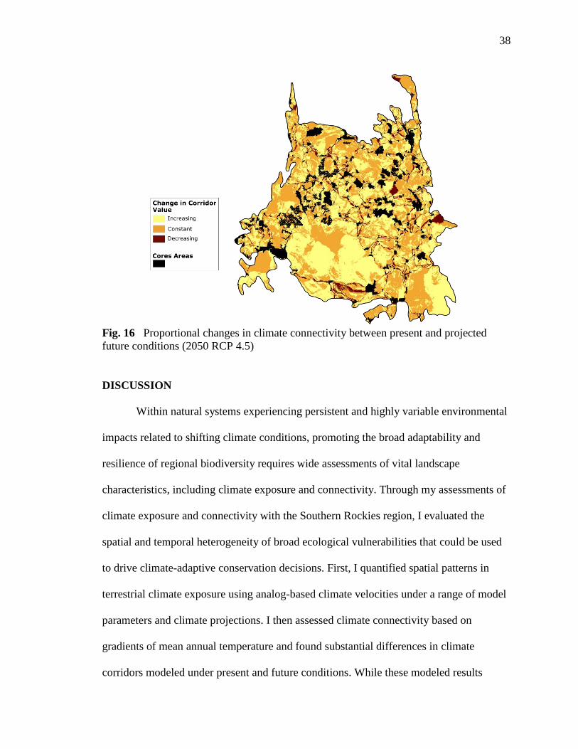
16 Proportional changes in climate connectivity between present and

projected future conditions (2050 RCP 4.5) .....................................................38

17 Spatial distributions of four Marxan inputs: a) conservation targets

(species of concern), b) risk (human land modification), c) climate

exposure, and d) climate connectivity ...............................................................50

18 Marxan outputs for conservation scenario #1 for minimizing climate

exposure: a) selection frequency and b) least-exposure run solution ...............53

19 Marxan outputs for conservation scenario #2 for maximizing climate

connectivity: a) selection frequency and b) most-connectivity run solution ....54

20 Adjoining high priority areas (climate corridors and climate refugia) .............55

21 Change in conservation priority (selection frequency) when accounting for

risk and ignoring risk in scenarios for a) minimizing climate exposure and

b) maximizing connectivity ..............................................................................56

22 Optimal climate refugia distribution relative to currently protected

planning units ....................................................................................................57

23 Protected planning unit characteristics versus the entire Southern

Rockies region, comparing a) climate exposure and b) modeled

conservation priority .........................................................................................57

24 The a) exposure cost and b) modeled conservation priority of the 50

largest contiguous protected areas, each over 250 km2 ....................................58

CHAPTER 1

INTRODUCTION

Natural systems are experiencing unprecedented pressures from never before

experienced rates of climate change. As patterns in climatic conditions shift and intensify,

species and ecosystems around the world have already started to respond physiologically

and ecologically to these changes (Walther et al., 2002). These numerous responses

include changes in species phenology (Parmesan & Yohe, 2003), restructuring of

community composition (Brown et al., 1997), and altitudinal and latitudinal shifts in

species ranges (Harsch et al., 2009; Chen et al., 2011). Furthermore, the impact of

climatic changes are not uniformly distributed across the landscape, varying along with

physiographical and ecological patterns such as latitude, altitude, and vegetation cover

(IPCC, 2014). Due in part to this heterogeneity of climate change impact, managers of

protected natural systems are confronted with the challenge of conserving species,

ecosystems, and other biological resources in an uncertain and rapidly changing world.

While current practices in global conservation continue to mandate the

identification and protection of areas primarily for their biological value, it has been

increasingly recommended that these conservation paradigms be adapted to explicitly

account for the impacts of climatic change (Hannah et al., 2002a; Heller & Zavaleta,

2008; CBD, 2016a, 2016b). However, in practice, the decisions made in designating

areas for conservation are still largely driven by the representation of current, static

ecological features, such as current species ranges or habitat types (Pressey et al., 2007;

Jones et al., 2016). This process has often failed to take into account the dynamic

biophysical nature of these systems, ignoring both their past and future proclivities for

2

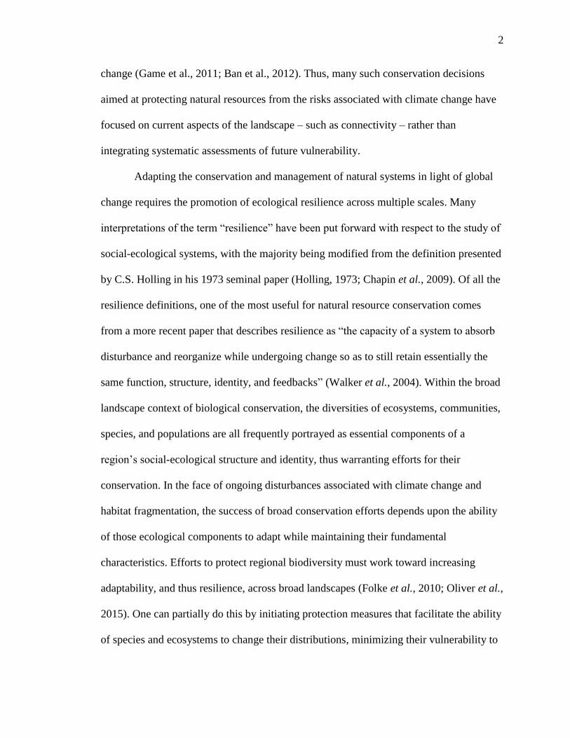
change (Game et al., 2011; Ban et al., 2012). Thus, many such conservation decisions

aimed at protecting natural resources from the risks associated with climate change have

focused on current aspects of the landscape – such as connectivity – rather than

integrating systematic assessments of future vulnerability.

Adapting the conservation and management of natural systems in light of global

change requires the promotion of ecological resilience across multiple scales. Many

interpretations of the term “resilience” have been put forward with respect to the study of

social-ecological systems, with the majority being modified from the definition presented

by C.S. Holling in his 1973 seminal paper (Holling, 1973; Chapin et al., 2009). Of all the

resilience definitions, one of the most useful for natural resource conservation comes

from a more recent paper that describes resilience as “the capacity of a system to absorb

disturbance and reorganize while undergoing change so as to still retain essentially the

same function, structure, identity, and feedbacks” (Walker et al., 2004). Within the broad

landscape context of biological conservation, the diversities of ecosystems, communities,

species, and populations are all frequently portrayed as essential components of a

region’s social-ecological structure and identity, thus warranting efforts for their

conservation. In the face of ongoing disturbances associated with climate change and

habitat fragmentation, the success of broad conservation efforts depends upon the ability

of those ecological components to adapt while maintaining their fundamental

characteristics. Efforts to protect regional biodiversity must work toward increasing

adaptability, and thus resilience, across broad landscapes (Folke et al., 2010; Oliver et al.,

2015). One can partially do this by initiating protection measures that facilitate the ability

of species and ecosystems to change their distributions, minimizing their vulnerability to

3

climate shifts.

In the field of conservation planning for climate change resilience, the broadest

level of decision making takes place when determining where and how to implement a

few key strategies for minimizing the overall impact of climate changes (Lawler, 2009;

Game et al., 2011; Jones et al., 2016). The first of these strategies has been to promote

resilience simply by preserving areas across diverse geophysical settings, such as broad

elevational and latitudinal gradients (Lawler, 2009). By protecting landscapes with

heterogeneous topography and geology, one captures much of the variation in climatic

and edaphic characteristics, providing organisms with the conditions necessary for them

to shift and adapt to variably shifting climates. Another major strategy of adaptation-

minded conservation targets the expansion of protected areas to incorporate climate

change refugia (Ashcroft, 2010; Gonzalez et al., 2010; Morelli et al., 2016). These

refugia serve as areas relatively buffered from climate impacts, enabling the persistence

of physical, ecological, and cultural resources. Rather than simply aim to maintain a

series of different refugia, a third main adaptation strategy involves enhancing landscape

connectivity. It is generally supported that the ability for organisms to move easily across

landscapes enhances the capacity for species to adapt to uncertain climatic changes and

their impacts (Heller & Zavaleta, 2008; Hannah, 2011; Beier, 2012).

While numerous robust methods for quantifying climate vulnerability exist,

generalizable data on climatic sensitivities and adaptive capacities that can be applied

across multiple species and ecosystems are frequently lacking. Thus, especially when

operating on broad scales that span multiple distinct ecological features, estimating

climate vulnerability primarily involves measuring climate exposure. Using climate

4

model projections that depict potential changes in temperature, precipitation, and other

biologically important climate metrics, one can derive simple approximations of climate

exposure based on overall magnitudes of change, such as increases in averaged

temperature variables (Parmesan & Yohe, 2003; Taylor et al., 2012a). However, other

methods for explicitly quantifying the intensity of climate change, such as the velocity of

climate change (hereafter “climate velocity”), can increase the biological-relevance of

abiotic climate exposure assessments (Loarie et al., 2009; Corlett & Westcott, 2013;

Burrows et al., 2014; Carroll et al., 2015). Climate velocity represents the minimum

speed at which an organism living in a certain area would theoretically have to travel in

order to maintain constant climate conditions in the future, given some projected long-

term shift in climate parameters (Loarie et al., 2009). While values of climate velocity

can be used as proxy measures of climate exposure for identifying potential climate

refugia, it is important to recognize that such abiotic measures ignore the actual presence

of ecological features of interest to conservation, including the distributions of threatened

species, cultural resources, and landscape facets (Morelli et al., 2016; Carroll et al.,

2017).

In efforts to reduce ecological vulnerabilities to climate shifts, the broad ability of

individual species to move across current and potential future landscapes – i.e. landscape

connectivity – must additionally be quantified, maintained, and enhanced (Heller &

Zavaleta, 2008; Beier, 2012). The importance of landscape connectivity for keeping

species, populations, communities, and ecosystems robust to the impacts of

environmental change has been readily observed across many systems (Tischendorf &

Fahrig, 2000a, 2000b; Prugh et al., 2008; Taylor et al., 2012b; Ayram et al., 2016).

5

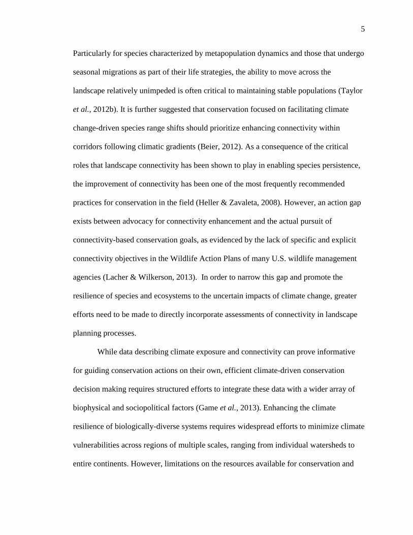
Particularly for species characterized by metapopulation dynamics and those that undergo

seasonal migrations as part of their life strategies, the ability to move across the

landscape relatively unimpeded is often critical to maintaining stable populations (Taylor

et al., 2012b). It is further suggested that conservation focused on facilitating climate

change-driven species range shifts should prioritize enhancing connectivity within

corridors following climatic gradients (Beier, 2012). As a consequence of the critical

roles that landscape connectivity has been shown to play in enabling species persistence,

the improvement of connectivity has been one of the most frequently recommended

practices for conservation in the field (Heller & Zavaleta, 2008). However, an action gap

exists between advocacy for connectivity enhancement and the actual pursuit of

connectivity-based conservation goals, as evidenced by the lack of specific and explicit

connectivity objectives in the Wildlife Action Plans of many U.S. wildlife management

agencies (Lacher & Wilkerson, 2013). In order to narrow this gap and promote the

resilience of species and ecosystems to the uncertain impacts of climate change, greater

efforts need to be made to directly incorporate assessments of connectivity in landscape

planning processes.

While data describing climate exposure and connectivity can prove informative

for guiding conservation actions on their own, efficient climate-driven conservation

decision making requires structured efforts to integrate these data with a wider array of

biophysical and sociopolitical factors (Game et al., 2013). Enhancing the climate

resilience of biologically-diverse systems requires widespread efforts to minimize climate

vulnerabilities across regions of multiple scales, ranging from individual watersheds to

entire continents. However, limitations on the resources available for conservation and

6

conflicts between competing management priorities typically make it unfeasible and

unrealistic to provide protections to all the least-vulnerable areas within any given

landscape. This forces managers to make tough decisions about where to prioritize the

allocation of limited resources, decisions often based on current management needs and

constraints rather than potential climate change vulnerabilities. While one can carry out

this process of selecting priority areas through a variety of methods, such as the

consultation of expert opinions, personal biases with respect to the direction of

management actions may produce inefficient paths for meeting conservation objectives.

As an alternative method to expert-led decision making process, systematic

landscape management (SLM) approaches can be utilized to improve the efficiency and

efficacy of spatial conservation efforts (Wilson et al. 2006). Systematic spatial

prioritization tools based on the concept of landscape complementarity, such as the

software program Marxan (Ball et al. 2009), are particularly suited for this task of

identifying of priority areas for conservation. These SLM strategies can be applied

toward achieving a variety of conservation goals, such as the protection of threatened

species or ecosystems. With Marxan in particular, this is done through an iterative

process that selects areas (“planning units”) that capture the spatial distribution of one’s

predefined conservation targets (e.g. species ranges) while also minimizing some “cost”

value across the landscape. This process produces networks of priority protected areas

characterized by a near-optimum balance between competing costs and conservation

goals. While the cost variable to be minimized in this model is frequently an economic

cost of restoring and managing the areas identified, one can alternatively seek to

minimize other values, such as the ecological “cost” of being more vulnerable to climate

7

shifts. Marxan further enables the conservation practitioner to directly incorporate a

broader suite of relevant biophysical and sociopolitical factors through the inclusion of

risk, the probability of a potential protected area failing to protect its targets.

Despite the versatility of SLM approaches and their potential for reconciling

competing interests in conservation efforts aimed at enhancing climate change resilience,

relatively little work has yet been done to explicitly address climate change impacts and

uncertainties in the field of systematic conservation prioritization (Jones et al., 2016).

Furthermore, very little climate-minded spatial prioritization research has addressed

human responses to climate change - such as land use changes driven by climate, and

their direct and indirect influences on conservation success (Faleiro et al., 2013;

Chapman et al., 2014; Jones et al., 2016). Given the ubiquitous roles that human actions

play in the viability of ecological systems, efforts to effectively conserve natural

resources in the face of climate change must continue to recognize the presence of

people. Strategies for SLM can adapt robust decision making frameworks for targeting

the protection of regional biodiversity in the face of widespread and rapid environmental

change.

Here I test the utility of spatial prioritization techniques for streamlining the

broad-scale conservation planning process in a manner that explicitly accounts for

multiple overlapping objectives, especially reduction of highly variable climate change

risks. Beginning in Chapter 2, I quantify broad metrics of climate change vulnerability

across my study region using two main metrics: climate velocity and climate gradient

connectivity. This fundamental assessment of vulnerability provides the basis for

proceeding with conservation prioritization driven by spatial heterogeneity in climate

8

impact. In Chapter 3, I use a Marxan decision framework to combine my vulnerability

estimates with threatened species ranges, existing protected areas, and land use risks. The

aim of the third Chapter is to spatially prioritize new areas based on their capacity for

maximizing regional resilience to climate shifts, and to assess the potential for existing

protected areas to withstand the dynamic impacts of climate change. I hope that the

decision making framework I describe will provide conservation practitioners with the

means to systematically and dynamically integrate ecological assessments of climate

vulnerability with the various social, economic, and political factors that also contributing

to long-term environmental resilience.

Study Region

For the purposes of this study, I conducted my analyses across the entire

landscape of the Southern Rockies region, as delineated by the Southern Rockies

Landscape Conservation Cooperative (Figure 1; Southern Rockies Landscape

Conservation Cooperative, 2018). The Landscape Conservation Cooperatives (LCC)

Network is an association of 22 landscape-scale collaborative partnerships between

governmental and non-governmental agencies and stakeholders that aim to address

conservation issues crossing jurisdictional boundaries within regions of broad ecological

similarity (Landscape Conservation Cooperatives, 2014). The ecologically-defined extent

and broad scale of these interdisciplinary endeavors also makes them particularly

applicable as regions for the practice of climate-driven systematic landscape

management. As one of these partnerships, the Southern Rockies LCC was established

for the collective conservation and management of a vast, topographically diverse region

spanning seven states (Arizona, Colorado, Idaho, Nevada, New Mexico, Utah, and

9

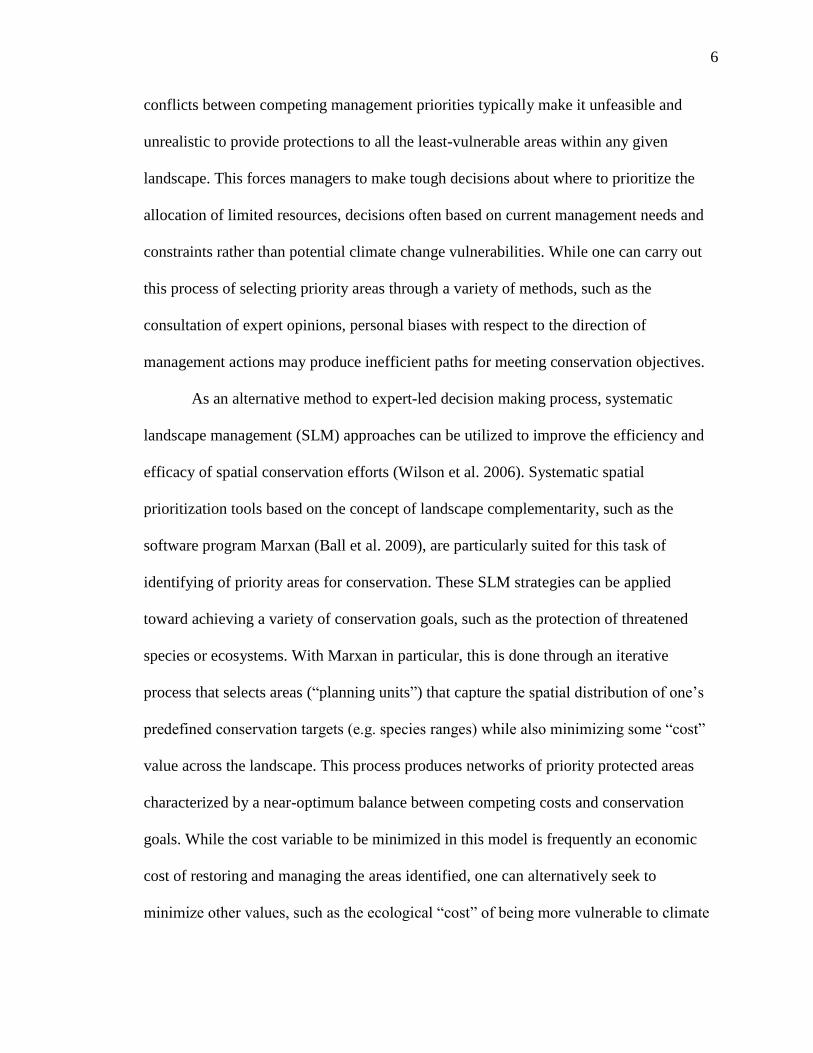
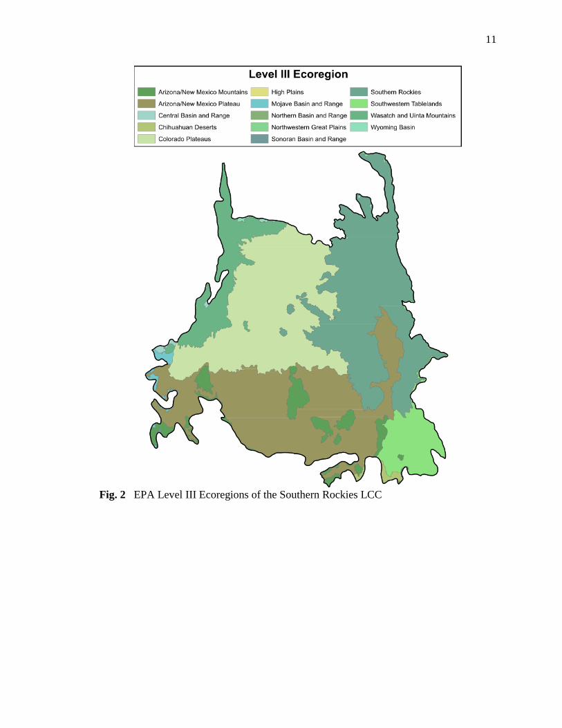
Wyoming). The ecosystems of the Southern Rockies LCC can be divided into more than

a dozen distinct regions ranging from the lowland Sonoran and Mojave deserts to the

highlands of the Southern Rocky Mountains, though the mountainous areas of Arizona,

Colorado, New Mexico, and Utah are most widely represented (Figure 2; Omernik &

Griffith, 2014). Though management priorities vary within the Southern Rockies LCC,

conservation efforts within the region primarily focus on five focal resources: cultural

resources, mule deer and elk, native fish, streamflow, and sagebrush-steppe ecosystems.

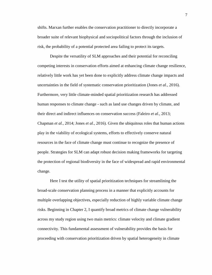
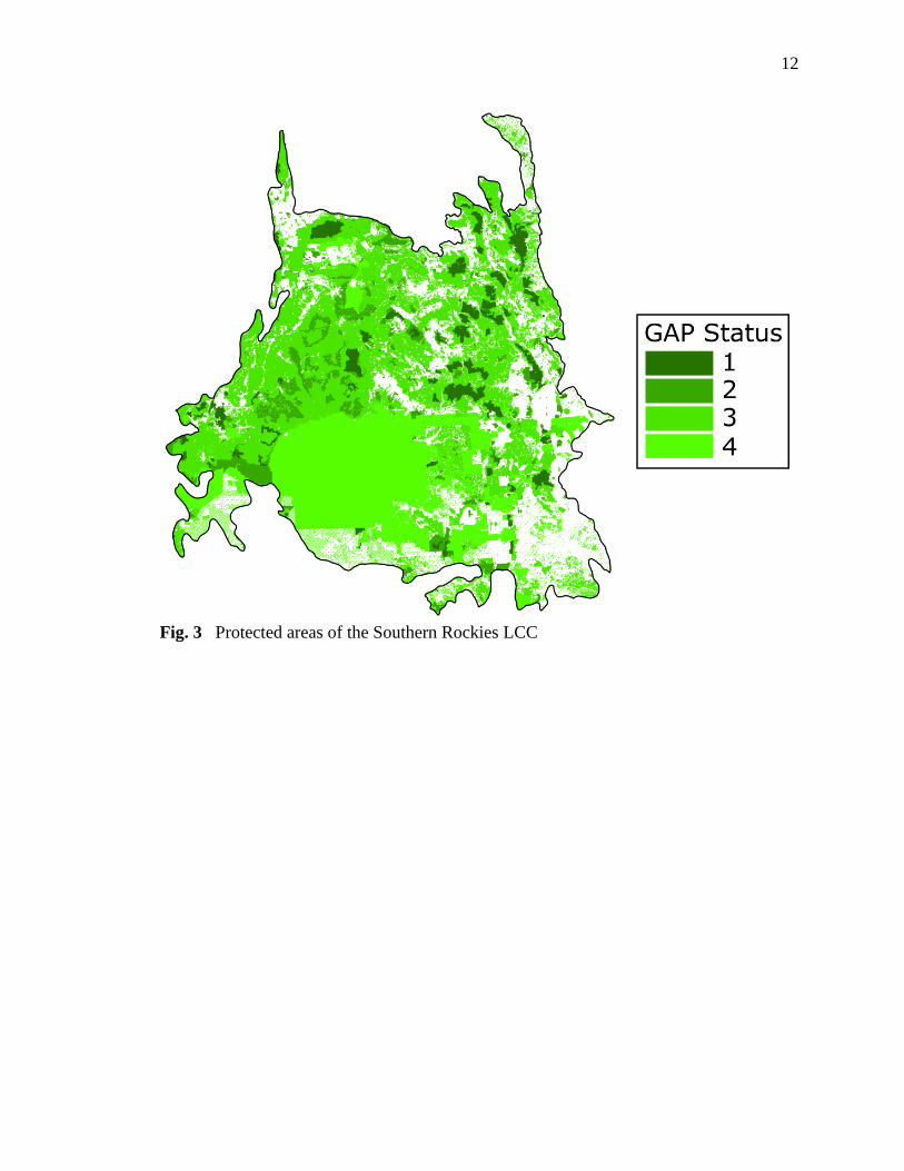
With 81.7105% of its extent listed within the USGS Protected Areas Database of

the United States (PADUS), the Southern Rockies region already receives widespread

landscape management. However, these areas receive different levels of protection,

allowing for varying degrees of management intensity, changes to ecological disturbance

regimes, and extractive uses (Figure 3). Of the PADUS areas, generally only those

designated with a GAP Status of 1 or 2 meet the global definition of a protected area by

the International Union for Conservation of Nature (IUCN). While these protected areas

(GAP Status 1 or 2) cover more than 67,000 square kilometers, they account for only

11.46% of the entire Southern Rockies region (Table 1). To reduce potential edge effects

when conducting certain analyses - namely the comparison of climate velocity results and

the modeling of climate connectivity – this study region was broadened to include the

geographic extent of a 100 kilometer buffer surrounding the Southern Rockies.

10

Fig. 1 Spatial Extent of the Southern Rockies Landscape Conservation Cooperative

(green) in the Western United States

11

Fig. 2 EPA Level III Ecoregions of the Southern Rockies LCC

12

Fig. 3 Protected areas of the Southern Rockies LCC

13

Table 1 USGS protected area GAP Status definitions and their coverage within the

Southern Rockies LCC

GAP

Status

Definition

(https://gapanalysis.usgs.gov/blog/iucn-

definitions/)

Area

Covered

(km2)

Percent of

Region

Covered

1

“An area having permanent protection from

conversion of natural land cover and a mandated

management plan in operation to maintain a natural

state within which disturbance events (of natural

type, frequency, intensity, and legacy) are allowed

to proceed without interference or are mimicked

through management.”

29,424 5.0527

2

“An area having permanent protection from

conversion of natural land cover and a mandated

management plan in operation to maintain a

primarily natural state, but which may receive uses

or management practices that degrade the quality

of existing natural communities, including

suppression of natural disturbance.”

37,636 6.4629

3

“Area having permanent protection from

conversion of natural land cover for the majority of

area. Subject to extractive uses of either broad,

low-intensity type (eg. Logging) or localized

intense type (eg. Mining). Confers protection to

federally listed endangered and threatened species

throughout the area.”

267,835 45.9929

4 “No known public/private institutional

mandates/legally recognized easements.” 140,938 24.202

14

CHAPTER 2

METRICS FOR PROMOTING CLIMATE CHANGE RESILIENCE

WITHIN THE SOUTHERN ROCKIES

ABSTRACT

In order for conservation to effectively adapt to climate change, it first requires a

broader understanding of how climate change impacts are likely distributed. Assessing

climate change risks and vulnerabilities across broad landscapes containing an array of

species, communities, and ecosystems requires estimates of climate change resilience that

are generally applicable across all relevant ecological features. Using broader metrics of

climate change exposure and connectivity, I evaluated the areas of the Southern Rockies

region based on their relative ability to enable the persistence of the region’s ecological

resources under a variety of projected climate shifts. Modeling climate velocities revealed

high spatial heterogeneity in climate exposure within the study regions. Though velocity-

based climate exposure varied depending on the bioclimatic variable used to calculate

them, the general spatial distribution of exposure was relatively consistent across multiple

future climate scenarios, with just the absolute value of velocity changing. Although the

absolute velocity changed, relative differences in velocity among locations remained the

constant, supporting the robustness of these metrics. Simulated climate connectivity

corridors provided further means for assessing the variability of adaptive capacity

throughout the region. With careful consideration of the assumptions of each, these proxy

metrics of climate change resilience demonstrate high potential for aiding in conservation

decision-making that spans multiple systems.

15

INTRODUCTION

Protecting multiple ecological resources from the dynamic impacts of climate

change requires conservation measures that promote the ability of those resources to

adapt to shifting climate across the landscape (Hannah et al., 2002b; Lawler, 2009;

Hannah, 2011). When seeking to quantify that adaptability, one must first understand the

distributions of climatic change impacts that influence vulnerabilities. Within this

context, vulnerability is typically defined as a function of exposure to climate shifts,

sensitivity to those shifts, and adaptive capacity (Dawson et al., 2011). Many climate-

adaptive strategies proposed and implemented in conservation are based on adequately

assessing the vulnerability of specific conservation targets, from individual taxa to broad

ecosystem types (Settele et al., 2014). When it comes to the protection of sensitive

species (a commonly sought after objective in conservation), climate vulnerability has

been assessed using an assortment of correlative, mechanistic, and trait-based approaches

(Pacifici et al., 2015). Of these approaches, those dealing with the modeling of past and

future species distribution shifts and climate change refugia – areas where species are less

vulnerable to climate shifts – have been the most extensively studied (Schloss et al.,

2012; Settele et al., 2014; Hannah et al., 2016; Jones et al., 2016; Morelli et al., 2016).

However, understanding the climatic vulnerabilities of each individual species or

ecosystem is time consuming and costly, typically making it difficult to apply this

approach across broad landscapes (Schloss et al., 2012). In order to more rapidly begin to

account for the pressures of climate change in the landscape conservation process, it may

be more prudent to focus on understanding less system-dependent differences in climatic

change exposure and adaptive capacity across landscapes.

16

Climate velocities represent a biologically relevant method for quantifying

climate change exposure in a way that is independent of the presence of specific taxa or

ecosystems. Instead, climate velocity uses the distributions of pre-defined climate

variables to calculate the rate at which any organism in a given area would theoretically

have to travel in order to get track climate shifts (Loarie et al., 2009). Fundamentally,

these velocities can be quantified simply using spatial and temporal gradients in climate

conditions (Loarie et al., 2009; Burrows et al., 2011, 2014; Dobrowski et al., 2013). For

additional ecological relevance, climate velocities can be also assessed on the basis of

future climate analogs, land units that are expected to have future climate conditions that

match with the conditions of areas within the present landscape (Carroll et al., 2015;

Hamann et al., 2015). Across an entire landscape of gridded climate cells, analog-based

climate velocity is calculated by taking each individual cell, pairing it with the nearest

cell projected to have matching climate in the future, and then dividing the geographic

distance between those two cells by the time difference between present and future time

periods (Hamann et al., 2015).

In order to broadly reduce climate change vulnerabilities, one should also promote

connectivity, the ability of organisms to move across the landscape (Lawler, 2009;

Hannah, 2011). When evaluating landscape connectivity within the context of enabling

multiple species to shift their ranges in response to climate change impacts, it is often

recommended that protected corridors between core areas follow climatic gradients

(Beier, 2012; Nuñez et al., 2013). While landscape connectivity models based on

individual target species ranges and movement patterns can provide targeted insight into

the ability of that species to move within current landscapes, the mapping of climate-

17

based connectivity can further aid in identifying areas critical for reducing climatic

vulnerabilities, particularly where climate conditions are very different between core

areas (Beier, 2012). Given the careful parameterization of the models of climate

connectivity, the corridors resulting from such models can provide a greater

understanding of where capacity for adapting to climate change can be most effectively

enhanced.

Despite the oft-stated importance of accounting for climate exposure and

connectivity in landscape conservation and management, the processes for evaluating

these multiple metrics associated with climate change resilience have not been widely

implemented in an integrative manner that can be applied toward broad conservation

decision-making. Here I specifically assess the landscape condition of the Southern

Rockies region based on climate velocities and on climate gradient connectivity between

major protected areas. To incorporate climate change uncertainties into my assessments, I

repeated my analyses across multiple projected climate conditions, including two

representative concentration pathways (RCP 4.5 and 8.5) and two time future time

periods from the Coupled Model Intercomparison Project Phase 5 (CMIP5) of the 5th

IPCC Assessment Report (IPCC, 2014). By comparing relative patterns of climate

exposure and connectivity across an array of modeling parameters, I was further able to

evaluate the robustness of the simulation models that I utilized.

METHODS

Climate Data

Spatial data depicting the current and projected climate conditions across North

America were obtained online from the climate database of the AdaptWest Project (Wang

18

et al., 2016). All of these climate datasets were developed using the ClimateNA software

package, which uses an approach based on localized elevation adjustments to downscale

broad-scale past, present, and future climate datasets to a finer (1 km) resolution at

multiple timescales. In addition to providing downscaled, monthly point-estimates for

both temperature and precipitation, the software produces a set of 27 derived climatic

variables of potential biological relevance, including chilling degree days, growing

degree days, and mean temperature of the warmest month. I primarily used two of these

bioclimatic variables – mean annual temperature (MAT) and mean annual precipitation

(MAP) – in my subsequent analyses. These two metrics were chosen to broadly

characterize climate conditions due to their close spatial correlation with other related

variables of ecological significance within North America, including summer

temperatures (Jones & Kelly, 1983; Koenig, 2002).

To reduce potential uncertainties associated with the use of climate predictions for

conservation management applications, my analyses of climate exposure and connectivity

were repeated under a range of scenarios that incorporate four climate projections.

Current climate conditions represent average recorded values from a 1981-2010 reference

climate period. Future climate data was obtained for two time periods: 2041-2070 and

2071-2100 (hereafter referred to as 2050s and 2080s, respectively). All future climate

projections are based on an average ensemble of 15 general circulation models (GCMs) –

CanESM2, ACCESS1.0, IPSL-CM5A-MR, MIROC5, MPI-ESM-LR, CCSM4,

HadGEM2-ES, CNRM-CM5, CSIRO Mk 3.6, GFDL-CM3, INM-CM4, MRI-CGCM3,

MIROC-ESM, CESM1-CAM5, GISS-E2R – included in the Coupled Model

Intercomparison Project Phase 5 (CMIP5) of the 5th IPCC Assessment Report (IPCC,

19

2014; Wang et al., 2016). This model ensemble was built from climate projections under

two distinct representative concentration pathways: RCP 4.5 and RCP 8.5. Whereas the

scenario under RCP 4.5 is characterized by a stabilization of radiative forcing and

represents a “middle-of-the-road” case for changing climate, RCP 8.5 corresponds to a

scenario where climate conditions are the result of continued acceleration of greenhouse

gas emissions in the absence of an effective climate change policy, and is often referred

to as “business as usual” (Riahi et al., 2011; Thomson et al., 2011).

Climate Exposure

To demonstrate the process of evaluating landscape components based on their

relative climate exposure, I calculated analog-based climate velocities for all of North

America. In order to compare changes in exposure of different climate variables, I

calculated climate velocities using mean annual temperature and mean annual

precipitation – both individually and in combination. All calculations and analyses were

conducted using R Version 3.3.2 (R Core Team, 2016) and ESRI ArcGIS. R-code used

for the calculation of climate velocities was adapted from R script algorithms provided by

Hamann et al. (2015) as part of the AdaptWest Project (Hamann et al., 2015). This

analog-based method of calculating climate velocity requires that the user set a threshold

value for each climate variable, a threshold that determines how similar the climate

values of current and future areas must be in order to be considered analogs of one

another (e.g. within 0.5°C). A smaller climate threshold indicates an increased precision

for a particular climate metric, and will tend to increase the distance that organisms

would need to travel in order to reach a future analog climate, resulting in greater climate

velocities (Hamann et al., 2015).

20

To investigate the relationship between climate threshold and the distance

between analogs, and thus determine an appropriate threshold both for mean annual

temperature and for mean annual precipitation, I repeated forward velocity calculations

under a range of threshold values within a single climate projection (2080s RCP 4.5). The

sensitivity of temperature-based velocity was tested using 12 thresholds between ±

0.025°C and 1°C and tests for the sensitivity of precipitation-based velocity were

conducted using 10 thresholds between ± 1 mm and 50 mm. From the results of this

sensitivity analysis, I selected a single threshold for each climate variable that was used

to obtain all remaining velocity results.

For each of mean annual temperature, mean annual precipitation, and the

multivariate combination of the two, I produced forward climate velocity raster datasets

for all of North American under all four combined climate projections (2050s RCP 4.5,

2050s RCP 8.5, 2080s RCP 4.5, and 2080s RCP 8.5) and compared their spatial

distributions. I then clipped every continental dataset down to the buffered extent of the

Southern Rockies and its immediate surroundings. All areas for which climate velocity

values could not be calculated – i.e. pixels with “no analog” climate – were reassigned

values equal to the maximum velocity within the clipped spatial extent. Similarities in the

patterns of velocity-based climate exposure estimates were quantitatively compared by

looking at the spatial concordance between values, using the following process. First, I

subset each of the two maps of climate velocity being compared into 10 rasters based on

the quantiles of their individual values. Then, working one quantile at a time (10%, 20%,

etc.), I overlaid each pair of split rasters and calculated the total number and percentage

of overlapping pixels. The resulting overlap between paired quantiles was then used to

21

represent the spatial agreement between the two maps. This process was repeated to make

three pairwise comparisons between velocity maps based on contrasting climate metrics

(temperature, precipitation, multivariate), eighteen comparisons of velocity under the four

climate projection (six for each climate metric).

Climate Connectivity

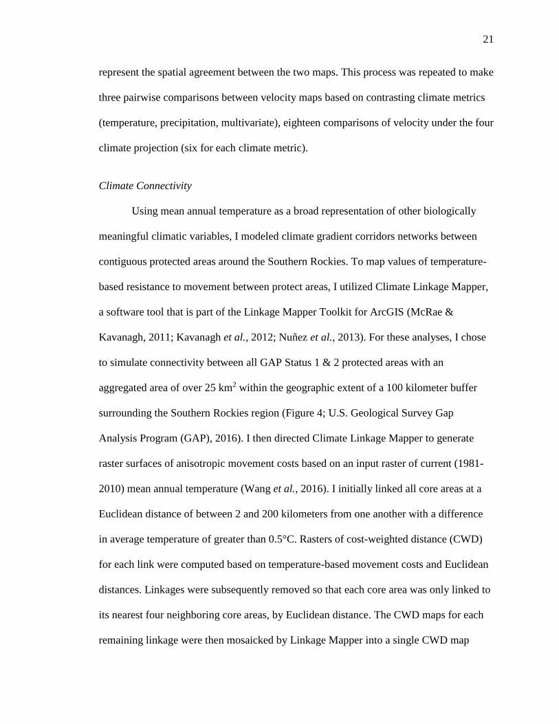
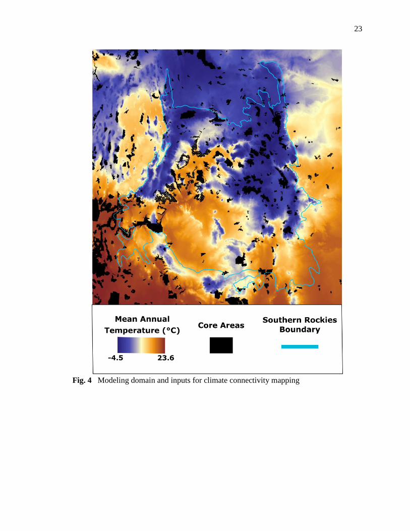
Using mean annual temperature as a broad representation of other biologically

meaningful climatic variables, I modeled climate gradient corridors networks between

contiguous protected areas around the Southern Rockies. To map values of temperature-

based resistance to movement between protect areas, I utilized Climate Linkage Mapper,

a software tool that is part of the Linkage Mapper Toolkit for ArcGIS (McRae &

Kavanagh, 2011; Kavanagh et al., 2012; Nuñez et al., 2013). For these analyses, I chose

to simulate connectivity between all GAP Status 1 & 2 protected areas with an

aggregated area of over 25 km2 within the geographic extent of a 100 kilometer buffer

surrounding the Southern Rockies region (Figure 4; U.S. Geological Survey Gap

Analysis Program (GAP), 2016). I then directed Climate Linkage Mapper to generate

raster surfaces of anisotropic movement costs based on an input raster of current (1981-

2010) mean annual temperature (Wang et al., 2016). I initially linked all core areas at a

Euclidean distance of between 2 and 200 kilometers from one another with a difference

in average temperature of greater than 0.5°C. Rasters of cost-weighted distance (CWD)

for each link were computed based on temperature-based movement costs and Euclidean

distances. Linkages were subsequently removed so that each core area was only linked to

its nearest four neighboring core areas, by Euclidean distance. The CWD maps for each

remaining linkage were then mosaicked by Linkage Mapper into a single CWD map

22

representing the temperature-based cost-of-movement. Areas with low movement cost

were then interpreted as having high value as climate gradient corridors (i.e. high

connectivity), while areas with high movement costs corresponded to low connectivity.

To evaluate the potential effect of climate shifts on connectivity between existing

protected areas in the Southern Rockies, I additionally modeled corridors and flow under

two projected future distributions of mean annual temperature (2050s RCP 4.5 and RCP

8.5), which I then compared to current corridors. Overall differences in model outputs

(resistance values) under each climate projection were used to infer potential changes in

climate connectivity under alternative future conditions. Projected increases in an area’s

resistance values corresponded to decreases in the value of that area as a climate corridor.

23

Fig. 4 Modeling domain and inputs for climate connectivity mapping

24

RESULTS

Climate Exposure

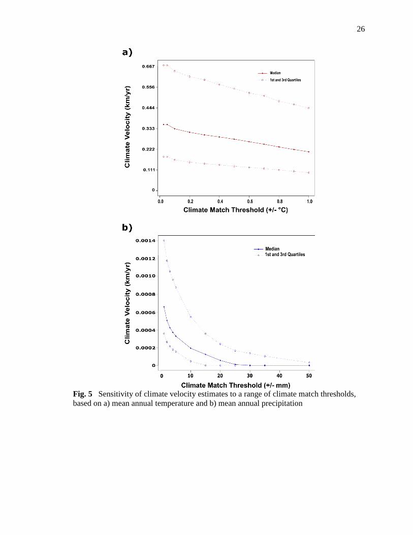
Forward climate velocity values modeled under a range of climate-match

thresholds for the 2080s RCP 4.5 climate projection revealed that velocities within the

buffered extent of the Southern Rockies study region respond in a relatively linear

fashion at large thresholds, with more rapid increases at small values (Figure 5). Tests of

temperature-based climate velocity showed that velocities within the study region

increase linearly as temperature threshold was reduced, with a slight inflection point at

around 0.2 °C (Figure 5a). Tests of the sensitivity of precipitation-based velocity were

conducted using 10 thresholds between ± 1 mm and 50 mm. Unlike the relatively linear

relationship between temperature and distance-to-match, as the precipitation threshold

was decreased, velocities increased exponentially (Figure 5b). Based on these analyses, I

chose to use ± 0.2°C for mean annual temperature and ± 5 mm for mean annual

precipitation in all subsequent univariate and multivariate velocity calculations, while

also aiming to determine the possible effects of these thresholds during later assessments

of relative exposure and priority.

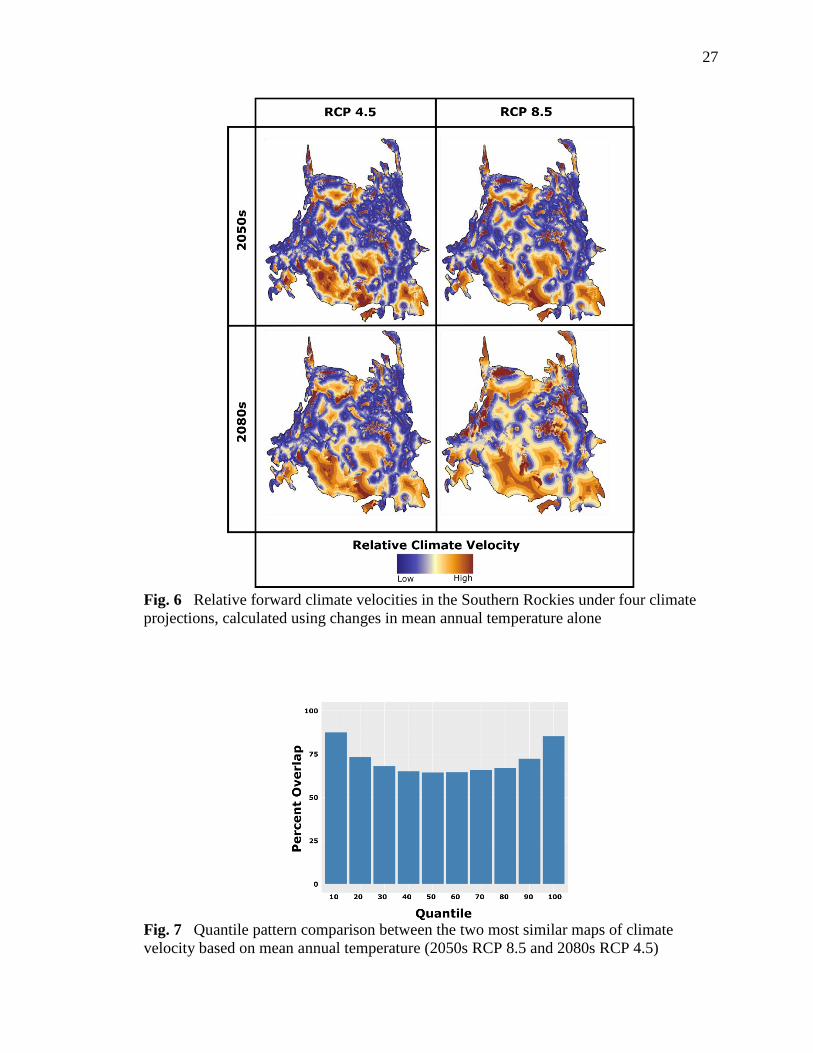
When used in isolation, mean annual temperature generated climate velocities that

varied considerably over the study region, but demonstrated similar spatial patterns in

exposure under all four climate projections (Figure 6). This spatial variation across the

study area suggests that certain areas will always be relatively severely impacted, while

others will be relatively lightly impacted by future changes in mean annual temperature.

The lowest absolute climate velocities based on mean annual temperature were seen

using the 2080s RCP 4.5 projection (mean = 0.0054, SD = 0.0063), while the highest are

25

observed in the 2050s RCP 8.5 projection (mean = 0.0131, SD = 0.0157). While

velocities under all four projections demonstrated a high degree of similarity in their

patterns – measured using percent overlap between 10th quantiles – considerable

differences were observable (Figure 7). In particular, the velocity results of the 2080 RCP

8.5 projection showed the least pattern similarity to other climate projections, especially

with the 2050 RCP 4.5 (mean quantile overlap = 19.67%). Quantile overlap was greatest

between the 2050 RCP 8.5 and 2080 RCP 4.5 projections (mean = 71.28%). However,

the areas with the highest and lowest climate velocity (top and bottom quantiles) appear

to have retained the highest amount of spatial overlap (Figure 7). Therefore, although

these sensitivity analyses comparing across climate projections shows some quantitative

differences in velocities, the relative exposure and importance of different areas remains

consistent.

26

Fig. 5 Sensitivity of climate velocity estimates to a range of climate match thresholds,

based on a) mean annual temperature and b) mean annual precipitation

27

Fig. 6 Relative forward climate velocities in the Southern Rockies under four climate

projections, calculated using changes in mean annual temperature alone

Fig. 7 Quantile pattern comparison between the two most similar maps of climate

velocity based on mean annual temperature (2050s RCP 8.5 and 2080s RCP 4.5)

28

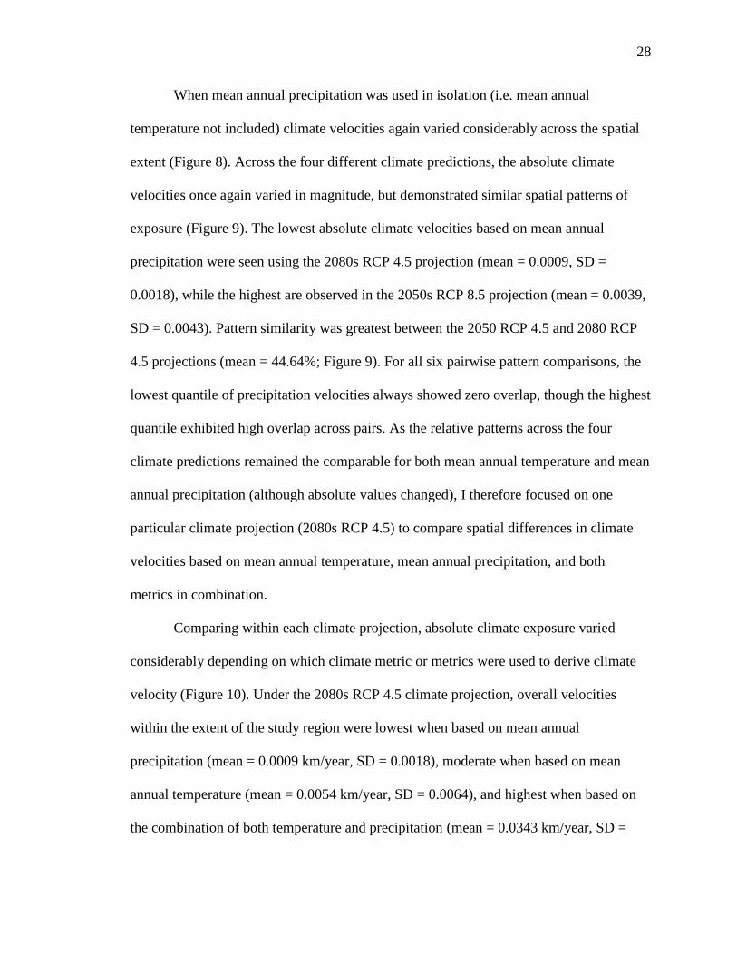
When mean annual precipitation was used in isolation (i.e. mean annual

temperature not included) climate velocities again varied considerably across the spatial

extent (Figure 8). Across the four different climate predictions, the absolute climate

velocities once again varied in magnitude, but demonstrated similar spatial patterns of

exposure (Figure 9). The lowest absolute climate velocities based on mean annual

precipitation were seen using the 2080s RCP 4.5 projection (mean = 0.0009, SD =

0.0018), while the highest are observed in the 2050s RCP 8.5 projection (mean = 0.0039,

SD = 0.0043). Pattern similarity was greatest between the 2050 RCP 4.5 and 2080 RCP

4.5 projections (mean = 44.64%; Figure 9). For all six pairwise pattern comparisons, the

lowest quantile of precipitation velocities always showed zero overlap, though the highest

quantile exhibited high overlap across pairs. As the relative patterns across the four

climate predictions remained the comparable for both mean annual temperature and mean

annual precipitation (although absolute values changed), I therefore focused on one

particular climate projection (2080s RCP 4.5) to compare spatial differences in climate

velocities based on mean annual temperature, mean annual precipitation, and both

metrics in combination.

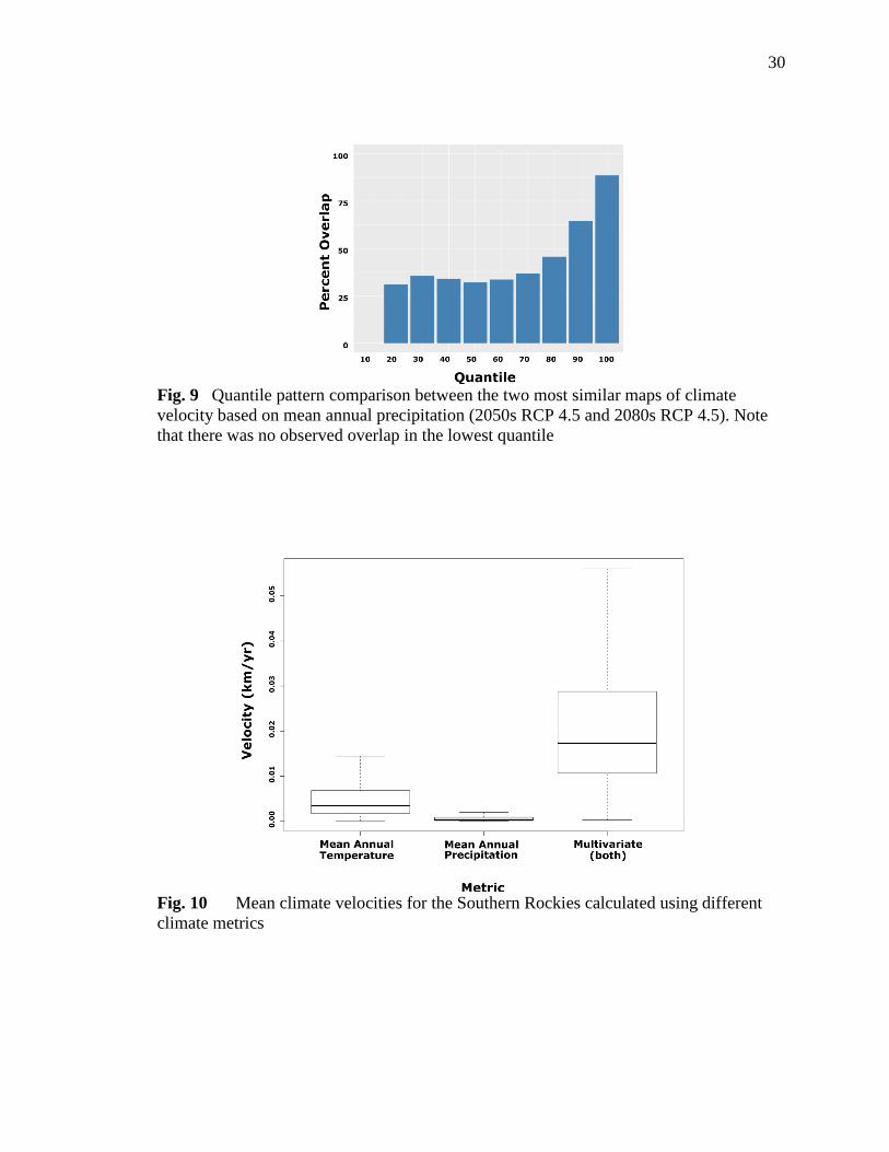
Comparing within each climate projection, absolute climate exposure varied

considerably depending on which climate metric or metrics were used to derive climate

velocity (Figure 10). Under the 2080s RCP 4.5 climate projection, overall velocities

within the extent of the study region were lowest when based on mean annual

precipitation (mean = 0.0009 km/year, SD = 0.0018), moderate when based on mean

annual temperature (mean = 0.0054 km/year, SD = 0.0064), and highest when based on

the combination of both temperature and precipitation (mean = 0.0343 km/year, SD =

29

0.0716). Across the entire study region, climate velocities were generally greater when

derived from two metrics simultaneously than when either of the metrics were treated in

isolation. This was to be expected given that the criteria for two areas being climate

analogs have been greatly narrowed, since they are now being dictated by two climate

parameters whose relative velocities have very distinct spatial patterns (Figures 11a and

11b).

Fig. 8 Relative forward climate velocities in the Southern Rockies under four climate

projections, calculated using changes in mean annual precipitation alone

30

Fig. 9 Quantile pattern comparison between the two most similar maps of climate

velocity based on mean annual precipitation (2050s RCP 4.5 and 2080s RCP 4.5). Note

that there was no observed overlap in the lowest quantile

Fig. 10 Mean climate velocities for the Southern Rockies calculated using different

climate metrics

31

When climate velocities were based on climate analogs of both mean annual

temperature and mean annual precipitation together, the spatial distribution of climate

velocities was substantially different than that observed when treating either metric in

isolation (Figure 11c). When both climate metrics used simultaneously in calculating

velocities, the patterns of exposure are seemingly composed of a combination of the high

velocity areas seen when each of the individual metrics are used. For example, in Figure

11c, the high climate velocities observed for the Uinta Mountains and the Colorado

Rockies appear to correspond with the high velocity areas seen in Figure 11a, while the

high velocities seen in the southern parts of the region also line up with those in Figure

11b. However, pattern similarity between velocity maps was generally low, with the

greatest being between temperature-based velocity and the multivariate velocity (mean

quantile overlap = 13.66%; Figure 12). Similarity was even lower between temperature

velocity and precipitation velocity (mean = 9.56%) and between precipitation velocity

and multivariate velocity (mean = 8.40%). This would suggest that differences in mean

annual temperature drive the patterns of multivariate velocity more strongly than

differences in mean annual precipitation. Generally, the differences in the distribution of

high and low velocity areas observed among the three maps indicate the potential

importance of guiding climate-related management decisions using the variable or

variables that are most appropriate for one’s particular question.

32

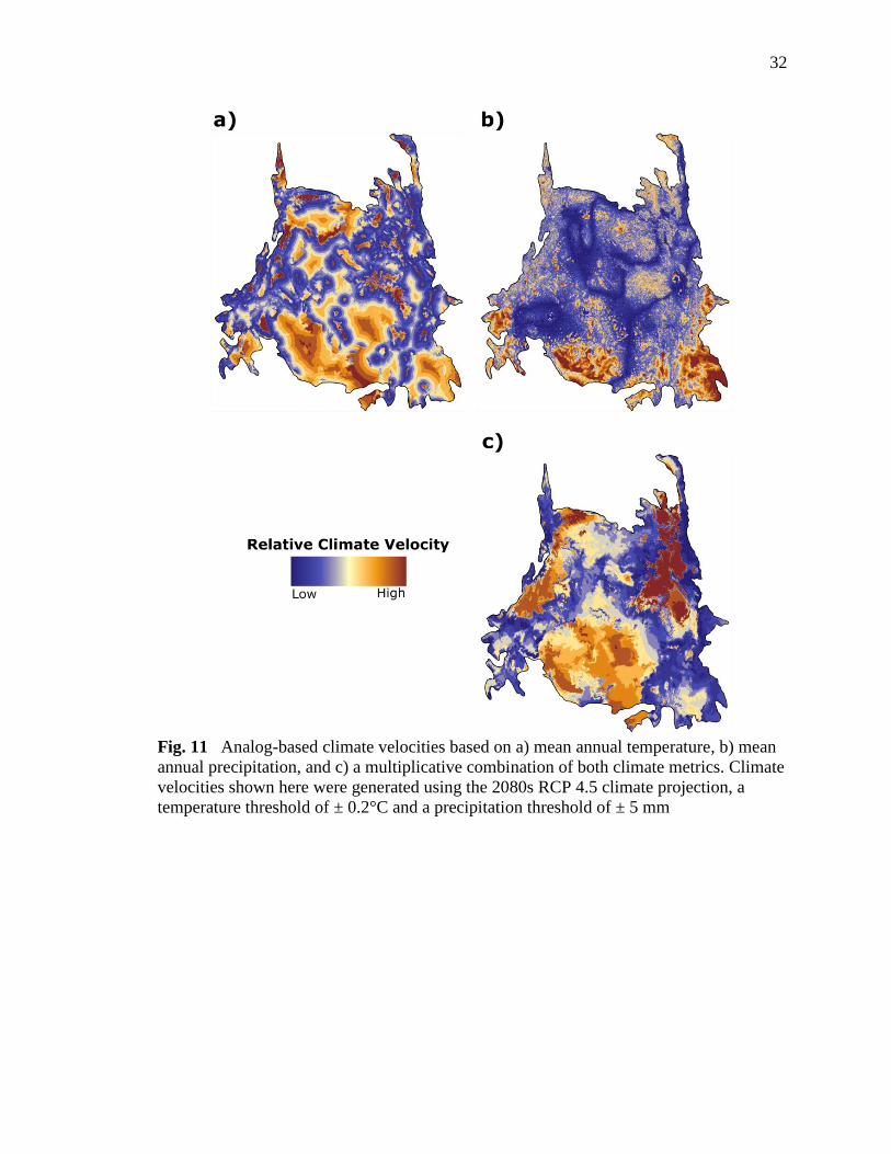
Fig. 11 Analog-based climate velocities based on a) mean annual temperature, b) mean

annual precipitation, and c) a multiplicative combination of both climate metrics. Climate

velocities shown here were generated using the 2080s RCP 4.5 climate projection, a

temperature threshold of ± 0.2°C and a precipitation threshold of ± 5 mm

33

Fig. 12 Similarity between climate velocity patterns generated using contrasting metrics

a) temperature vs. precipitation, b) temperature vs. multivariate, and c) precipitation vs.

multivariate

34

Climate Connectivity

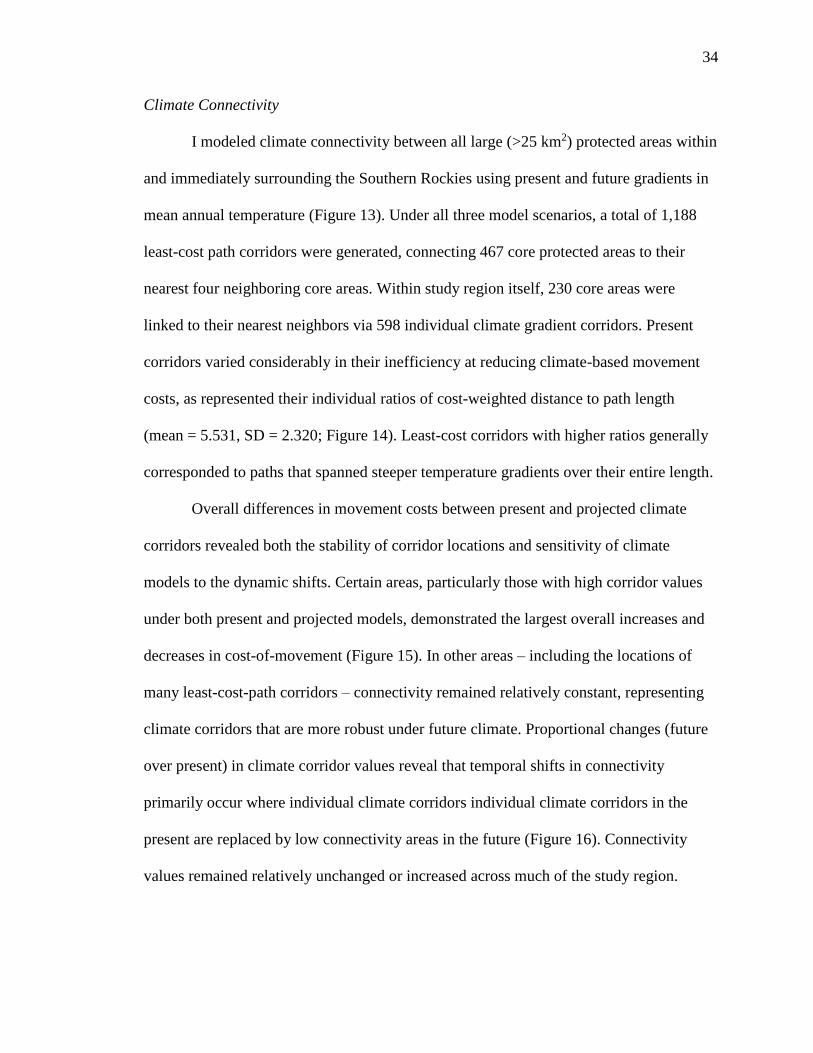
I modeled climate connectivity between all large (>25 km2) protected areas within

and immediately surrounding the Southern Rockies using present and future gradients in

mean annual temperature (Figure 13). Under all three model scenarios, a total of 1,188

least-cost path corridors were generated, connecting 467 core protected areas to their

nearest four neighboring core areas. Within study region itself, 230 core areas were

linked to their nearest neighbors via 598 individual climate gradient corridors. Present

corridors varied considerably in their inefficiency at reducing climate-based movement

costs, as represented their individual ratios of cost-weighted distance to path length

(mean = 5.531, SD = 2.320; Figure 14). Least-cost corridors with higher ratios generally

corresponded to paths that spanned steeper temperature gradients over their entire length.

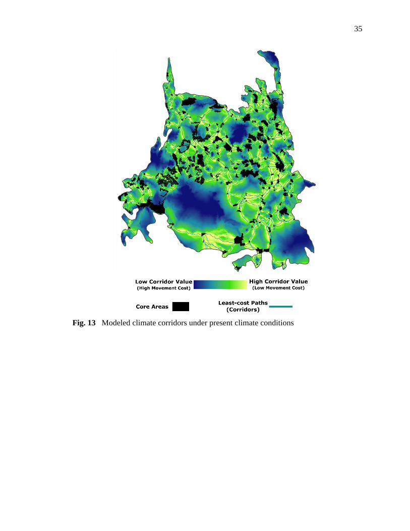
Overall differences in movement costs between present and projected climate

corridors revealed both the stability of corridor locations and sensitivity of climate

models to the dynamic shifts. Certain areas, particularly those with high corridor values

under both present and projected models, demonstrated the largest overall increases and

decreases in cost-of-movement (Figure 15). In other areas – including the locations of

many least-cost-path corridors – connectivity remained relatively constant, representing

climate corridors that are more robust under future climate. Proportional changes (future

over present) in climate corridor values reveal that temporal shifts in connectivity

primarily occur where individual climate corridors individual climate corridors in the

present are replaced by low connectivity areas in the future (Figure 16). Connectivity

values remained relatively unchanged or increased across much of the study region.

35

Fig. 13 Modeled climate corridors under present climate conditions

36

Fig. 14 Least-cost paths (corridors) by efficiency, represented using the ratio between

cost-weighted distance (CWD) and the Euclidean distance of the path

37

Fig. 15 Overall in climate-based movement costs between present and projected future

conditions (2050 RCP 4.5). Red areas correspond to large increases in costs (decreases in

corridor value), whereas blue corresponds to decreases in costs (increases in corridor

value)

38

Fig. 16 Proportional changes in climate connectivity between present and projected

future conditions (2050 RCP 4.5)

DISCUSSION

Within natural systems experiencing persistent and highly variable environmental

impacts related to shifting climate conditions, promoting the broad adaptability and

resilience of regional biodiversity requires wide assessments of vital landscape

characteristics, including climate exposure and connectivity. Through my assessments of

climate exposure and connectivity with the Southern Rockies region, I evaluated the

spatial and temporal heterogeneity of broad ecological vulnerabilities that could be used

to drive climate-adaptive conservation decisions. First, I quantified spatial patterns in

terrestrial climate exposure using analog-based climate velocities under a range of model

parameters and climate projections. I then assessed climate connectivity based on

gradients of mean annual temperature and found substantial differences in climate

corridors modeled under present and future conditions. While these modeled results

39

demonstrated sensitivity to certain inputs – especially climate variables – they were also

validated through their robustness across multiple uncertain climate projections.

When making conservation decisions based on any sort of broad landscape-scale

analyses such as these, it is critical to remain mindful of the fundamental assumptions of

one’s methodological approaches. For one, assessments of climate exposure and

connectivity based on climate predictions depend on the use of only a select few climate

variables – such as mean annual temperature and precipitation – that are assumed to be

the closest approximations of many other more biologically-meaningful variables. Since

it can be readily demonstrated that patterns in climate shifts and their impacts vary

depending on which aspect of climate is being looked at, practitioners of landscape

climate assessment and conservation prioritization must be careful about which climate

variables they select. On this note, one must keep in mind that certain climate variables,

particularly temperature-based variables, have much lower uncertainty due to the greater

degree of agreement between the predictions of global and regional climate models of

temperature, relative to those for precipitation (Hawkins & Sutton, 2009; Flato et al.,

2013). This suggests that temperature variables would be more reliable as a basis for

management actions. Secondly, conducting analyses at broad spatial resolutions of 1 km2

and larger ignores much of the finer scale variation in climate vulnerability. Through the

use of coarser spatial resolutions, one cannot determine the presence or absence of small-

scale climate microrefugia, though large-scale macrorefugia can still be identified

(Ashcroft, 2010). Thirdly, it is important to note the considerable differences between the

four climate projections that were used to calculate climate velocity and connectivity.

Vulnerability assessments utilizing climate model projections over longer time periods

40

(e.g. the 2080s) are inherently less certain than those for shorter time periods (e.g. the

2050s) and do not align as well with shorter time-scales of ecology and human decision

making (Chapman et al., 2014). Additionally, there is considerable uncertainty of human

behavior in the trajectories that will lead to the contrasting emissions scenarios (RCP 4.5

vs. RCP 8.5). However, validating exposure and connectivity models under multiple

climate projections has served to evaluate the robustness of these models to uncertain

future conditions. These assumptions, among many others, highlight some areas of

caution that must be carefully considered by managers when making decisions about

where best to undergo new conservation actions.

Despite the caveats associated with the use of generalized landscape approaches

for guiding conservation making, they provide important information that can be helpful

for natural systems managers looking to prepare their systems for the ongoing impacts of

rapid climate change. Across Utah, the Intermountain West, and regions around the

world, biological systems are expected to respond to climate change over vast spatial

scales. In order to conserve the diversity of those systems, greater efforts must be made to

explicitly incorporate the distribution of climate change impacts into conservation efforts.

Moving forward, I believe that the use of systematic landscape planning strategies based

on climate vulnerability and connectivity will provide an efficient method for prioritizing

conservation actions in a manner that is directly applicable to aiding real-world

management efforts to tackle the impacts of climate change.

41

CHAPTER 3

SYSTEMATICALLY INCORPORATING CLIMATE RESILIENCE METRICS INTO

LANDSCAPE CONSERVATION

ABSTRACT

In the face of climate change, protected area conservation must explicitly account

for variability in the vulnerability of ecological systems to multiple shifting

environmental conditions. When prioritizing conservation across broad landscapes, it is

often prudent to focus on areas where low levels of climate exposure (refugia) and high

levels of connectivity (corridors) enhance the resilience of the overall system. While

broad metrics of exposure and connectivity can alone aid in identifying priority areas,

they often fail to account for the distributions of species and other ecological features

necessary for meeting management goals. Frameworks for spatially prioritizing

conservation to account for climate change impacts must be able to simultaneously

address management goals (e.g. species protection) and the factors affecting the

likelihood of achieving those goals. By integrating a wider variety of social-ecological

variables, systematic landscape planning strategies can be utilized to efficiently identify

priority areas for potential conservation. I estimated climate exposure and climate

connectivity within the US Southern Rockies region. I then used the software Marxan to

prioritize areas of minimal climate exposure and maximal connectivity, while

additionally accounting for the presence of species of interest, protected areas, and

environmental risks. Lastly, I evaluated the adaptability of existing protected areas by

comparing their characteristics with those of optimized climate refugia. This model

framework successfully identified priority climate refugia and corridors that also

42

contained the ranges of the region’s threatened wildlife species. Explicitly accounting for

the presence of human development as a risk to conservation success served to further

identify the highest priority areas. While some optimized climate refugia fell within

existing protected areas, the extent of the refugia aligned more closely with areas of

lowest exposure. While climate exposure and modeled priority were similar between the

entire protected area system and the overall region, they varied considerably within and

between individual protected areas. These results highlight the need for more thorough

spatial assessment of factors contributing to ecological vulnerabilities and likelihoods of

conservation success. I hope that the results and framework that I outline here will aid

managers in efficiently allocating conservation resources with the goal of promoting

ecological resilience.

INTRODUCTION

Though the establishment and management of widespread networks of protected

areas remains a central strategy for the conservation of ecological resources, it is unclear

how well these largely static systems will be able to bear the impacts of climate change

(Game et al., 2011; Ban et al., 2012). With individual protected areas already

experiencing unprecedented ecological shifts driven by climate change, their ability to

maintain climate characteristics within their borders appears compromised (Marris,

2011). Given that many of these smaller-scale protected landscapes will continue to

change, preserving biodiversity and other natural resources across wider regions

necessitates enhancement of landscape characteristics that allow for species to adapt,

making them more resilient to the impacts of climate (Hobbs et al., 2014).

While it remains important to consider whether current protected area systems can

43

survive the impacts of climate change, promoting regional climate resilience requires

evaluating new areas for potential conservation. Although present protected areas

demonstrate clear value to conservation here and now, it is likely that that value will

change in the future, and that better conservation outcomes could be produced through

altering protected area networks (Fuller et al., 2010). For instance, in the process of

evaluating landscape-level climate change resilience, it may be found that existing

protected areas contain optimal climate refugia. However, certain other protected areas

could alternatively exhibit the highest potential for being impacted by climate change,

with better climate refugia falling outside their current borders. In order to maintain or

even increase conservation values across broad regions, protected area systems could be

adapted to incorporate areas of limited climate vulnerability, namely the climate refugia

and corridors that enable organisms to seek out new, more suitable climates (Hannah,

2011).

The distributions of metrics closely associated with climate change vulnerability,

such as climate exposure and connectivity, play central roles in conservation decision

making processes designed to account for climate change. While numerous methods for

broadly evaluating climate change vulnerability already exist, they are typically

implemented on a case-by-case basis and their outputs require additional synthesis in

order to make the information more usable for decision makers. In the previous chapter I

demonstrated how estimations of climate velocities and connectivity can be used to

broadly assess vulnerability to climate change across entire landscapes. However, these

generalized metrics are notably limited in their ecological specificity in that they are

primarily based on abiotic parameters of climate change. For them to effectively guide

44

conservation decisions, these coarse filter metrics must be subsequently combined with

the biotic features that are of interest to conservation, such as threatened species (Beier,

2012). Otherwise, any landscape conservation efforts driven purely by climate impact

metrics may fail to meet conservation targets for actual species and ecosystems, as

evidenced by suboptimal results in the global protection of threatened species (Venter et

al., 2014). Thus, methodological frameworks are required for explicitly guiding

conservation based on ecological goals while also reducing climate vulnerabilities,

especially when those goals conflict with one another (Reside et al., 2017).

In having to reconcile multiple overlapping goals and management priorities,

whether climate-driven or not, conservation decisions must efficiently prioritize where

conservation actions should occur in order to make effective use of limited resources.

Fortunately, tools from the field of spatial prioritization – including the software package

Marxan (Ball et al., 2009) - have long been utilized for this purpose of simultaneously

achieving multiple conservation targets while incurring minimal costs (Wilson et al.,

2006). However, as addressed in Chapter 1, efforts to spatially prioritize conservation

based on climate change and its impacts have been rather limited (Jones et al., 2016).

While many of these studies have dealt with spatially prioritizing based on reducing

climate exposure, assessing climate refugia, and protecting diverse ecological landscapes

(Game et al., 2011; Ban et al., 2012; Levy & Ban, 2013; Carroll et al., 2017), significant

research gaps are evident. Notably, few studies have either incorporated multiple

conservation objectives or explicitly accounted for a multitude of stressors and risks

associated with climate change (Jones et al., 2016). There is an apparent need for

conservation decision frameworks that can integrate climate-related impacts with

45

contrasting management objectives across different systems.

In addition to explicitly and efficiently accounting for multiple competing

management targets, spatial prioritization for climate change must be able to account for

a wider variety of social, economic, and political risks, particularly on the sub-national

and regional scales at which landscape conservation planning occurs. Climate change is

one factor among many influencing the ability to conserve ecological resources. In order

to bridge gaps between climate-based conservation theory and practice, one must still

account for the anthropogenic activities that constrain conservation success (Heller &

Zavaleta, 2008). Despite this need, the direct and indirect effects associated with people

and their responses to climate change have been relatively understudied, particularly

when it comes to spatial prioritization (Faleiro et al., 2013; Chapman et al., 2014; Jones

et al., 2016). Given the undeniable global prevalence of anthropogenic influences on

biodiversity, new methods for spatially prioritizing conservation based on climate change

must be able to account for the risks to conservation success, particularly associated with

people (Game et al., 2013).

Especially in landscapes where vulnerabilities to climate change are highly

variable, strategies for systematic landscape planning can be utilized to efficiently meet

multiple conservation goals in a manner that explicitly integrates those vulnerabilities

with additional factors affecting conservation success. Based on the prior assessments of

metrics influencing climate vulnerability (exposure and connectivity), I used the software

program Marxan to systematically construct arrays of potential conservation networks

aimed at enhancing climate change resilience across the Southern Rockies region. I

further assessed how the characteristics of the resulting high priority conservation areas

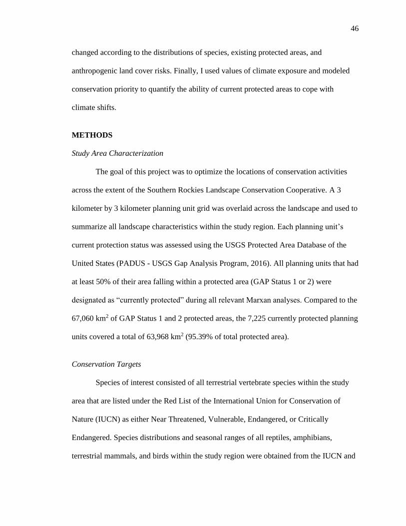
46

changed according to the distributions of species, existing protected areas, and

anthropogenic land cover risks. Finally, I used values of climate exposure and modeled

conservation priority to quantify the ability of current protected areas to cope with

climate shifts.

METHODS

Study Area Characterization

The goal of this project was to optimize the locations of conservation activities

across the extent of the Southern Rockies Landscape Conservation Cooperative. A 3

kilometer by 3 kilometer planning unit grid was overlaid across the landscape and used to

summarize all landscape characteristics within the study region. Each planning unit’s

current protection status was assessed using the USGS Protected Area Database of the

United States (PADUS - USGS Gap Analysis Program, 2016). All planning units that had

at least 50% of their area falling within a protected area (GAP Status 1 or 2) were

designated as “currently protected” during all relevant Marxan analyses. Compared to the

67,060 km2 of GAP Status 1 and 2 protected areas, the 7,225 currently protected planning

units covered a total of 63,968 km2 (95.39% of total protected area).

Conservation Targets

Species of interest consisted of all terrestrial vertebrate species within the study

area that are listed under the Red List of the International Union for Conservation of

Nature (IUCN) as either Near Threatened, Vulnerable, Endangered, or Critically

Endangered. Species distributions and seasonal ranges of all reptiles, amphibians,

terrestrial mammals, and birds within the study region were obtained from the IUCN and

47

BirdLife International (BirdLife International and Handbook of the Birds of the World,

2016; IUCN, 2016). The final distribution dataset consisted of the 36 ranges of 31

terrestrial wildlife species of interest (Appendix A), with the greatest diversity of species

located in southeastern corner of the region (Figure 17a). The amount of each species

range represented within each planning unit was calculated and proportional conservation

targets in all Marxan runs were then set as 20% of each species range, corresponding to a

mid-range landscape intactness threshold for forest species persistence (Betts & Villard,

2009). This 20% proportion was chosen to provide a moderately strict set of conservation

targets that also closely aligns with the 17% terrestrial landscape conservation objective

set through the Aichi Biodiversity Targets (CBD, 2016a). The penalty for failure to meet

an individual target – the species protection factor (SPF) in Marxan – was set to a value

of 10,000 for all species.

Risk

The distribution of risk to potential protected area success was estimated based on

the presence of human-modified land cover types in the National Land Cover Database

(Homer et al., 2015). Using the Spatial Analyst toolset in ArcGIS 10.4, I calculated the

total area and proportion of each NLCD classification within each planning unit. I then

quantified each planning unit’s overall modification intensity by aggregating the

percentages of all agricultural and developed land classifications, which included pasture,

hay, cultivated crops, and lands with variable intensities of development (Figure 17b).

These percentage of land modification were then directly applied to Marxan as the

probabilistic risk of planning unit failure, i.e. this is the percentage of the planning unit

that is unlikely to be primarily used for conservation of biodiversity.

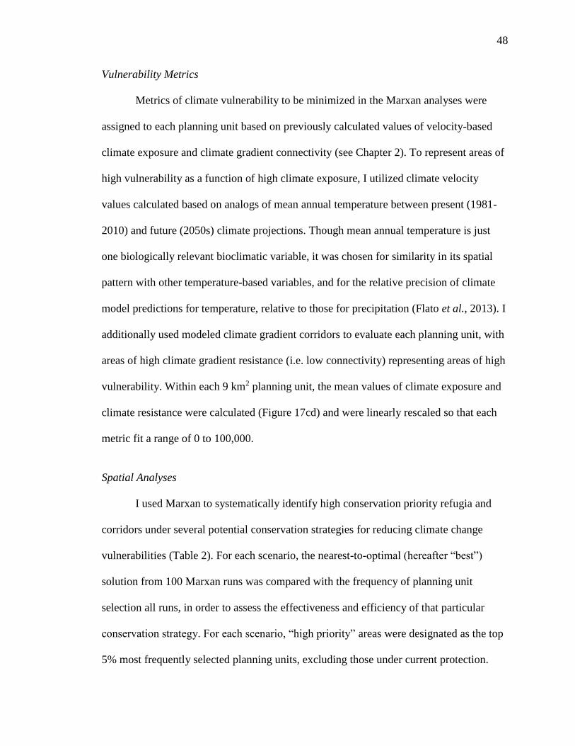
48

Vulnerability Metrics

Metrics of climate vulnerability to be minimized in the Marxan analyses were

assigned to each planning unit based on previously calculated values of velocity-based

climate exposure and climate gradient connectivity (see Chapter 2). To represent areas of

high vulnerability as a function of high climate exposure, I utilized climate velocity

values calculated based on analogs of mean annual temperature between present (1981-

2010) and future (2050s) climate projections. Though mean annual temperature is just

one biologically relevant bioclimatic variable, it was chosen for similarity in its spatial

pattern with other temperature-based variables, and for the relative precision of climate

model predictions for temperature, relative to those for precipitation (Flato et al., 2013). I

additionally used modeled climate gradient corridors to evaluate each planning unit, with

areas of high climate gradient resistance (i.e. low connectivity) representing areas of high

vulnerability. Within each 9 km2 planning unit, the mean values of climate exposure and

climate resistance were calculated (Figure 17cd) and were linearly rescaled so that each

metric fit a range of 0 to 100,000.

Spatial Analyses

I used Marxan to systematically identify high conservation priority refugia and

corridors under several potential conservation strategies for reducing climate change

vulnerabilities (Table 2). For each scenario, the nearest-to-optimal (hereafter “best”)

solution from 100 Marxan runs was compared with the frequency of planning unit

selection all runs, in order to assess the effectiveness and efficiency of that particular

conservation strategy. For each scenario, “high priority” areas were designated as the top

5% most frequently selected planning units, excluding those under current protection.

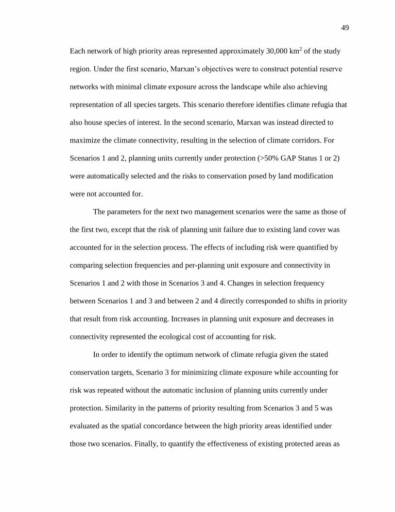
49

Each network of high priority areas represented approximately 30,000 km2 of the study

region. Under the first scenario, Marxan’s objectives were to construct potential reserve

networks with minimal climate exposure across the landscape while also achieving

representation of all species targets. This scenario therefore identifies climate refugia that

also house species of interest. In the second scenario, Marxan was instead directed to

maximize the climate connectivity, resulting in the selection of climate corridors. For

Scenarios 1 and 2, planning units currently under protection (>50% GAP Status 1 or 2)

were automatically selected and the risks to conservation posed by land modification

were not accounted for.

The parameters for the next two management scenarios were the same as those of

the first two, except that the risk of planning unit failure due to existing land cover was

accounted for in the selection process. The effects of including risk were quantified by

comparing selection frequencies and per-planning unit exposure and connectivity in

Scenarios 1 and 2 with those in Scenarios 3 and 4. Changes in selection frequency

between Scenarios 1 and 3 and between 2 and 4 directly corresponded to shifts in priority

that result from risk accounting. Increases in planning unit exposure and decreases in

connectivity represented the ecological cost of accounting for risk.

In order to identify the optimum network of climate refugia given the stated

conservation targets, Scenario 3 for minimizing climate exposure while accounting for

risk was repeated without the automatic inclusion of planning units currently under

protection. Similarity in the patterns of priority resulting from Scenarios 3 and 5 was

evaluated as the spatial concordance between the high priority areas identified under

those two scenarios. Finally, to quantify the effectiveness of existing protected areas as

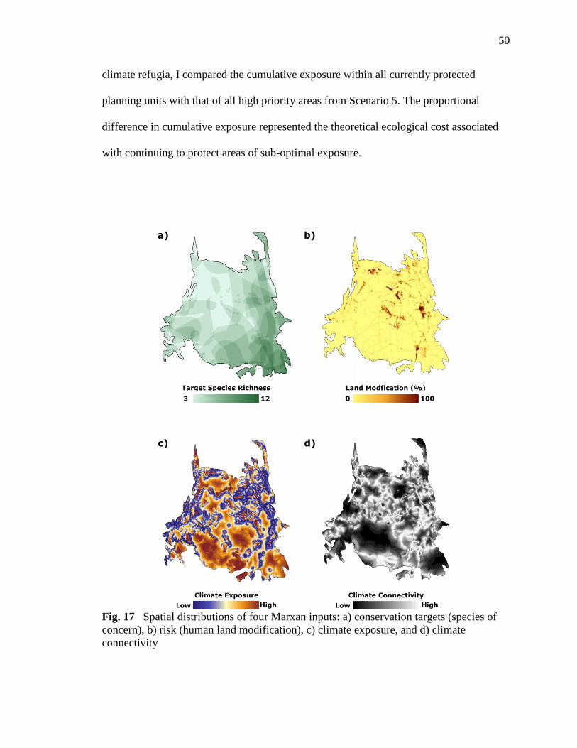
50

climate refugia, I compared the cumulative exposure within all currently protected

planning units with that of all high priority areas from Scenario 5. The proportional

difference in cumulative exposure represented the theoretical ecological cost associated

with continuing to protect areas of sub-optimal exposure.

Fig. 17 Spatial distributions of four Marxan inputs: a) conservation targets (species of

concern), b) risk (human land modification), c) climate exposure, and d) climate

connectivity

51

Table 2 Marxan parameters for each conservation scenario

Scenario Goal Risk Existing Protected

Areas Included?

1 Minimize exposure Ignored Yes

2 Maximize connectivity Ignored Yes

3 Minimize exposure Accounted for Yes

4 Maximize connectivity Accounted for Yes

5 Minimize exposure Accounted for No

RESULTS

Under the first management scenario aimed at minimizing climate exposure,

patterns in modeled conservation priority indicated the selection of new areas that have

both low climate exposure also meet species representation targets. In Scenario 1, areas

with the highest selection frequencies generally corresponded to areas with the lowest

climate exposure, though planning units were more often selected where the diversity of

targeted wildlife species was highest, particularly the southeastern and northeastern

portions of the region (Figure 18a). The mean exposure value of these high priority

planning units was about 9.3 times higher than planning units with the lowest 5% of

exposure values. This difference directly reflects the trade-off between minimizing

exposure and protecting one’s conservation targets. The areas selected in the best

(lowest-exposure) solution showed similar patterns to those in selection frequency

(Figure 18b). All Marxan runs under Scenario 1 – including the lowest-exposure solution

– met the representative conservation targets for all species.

Results from the maximum connectivity scenarios similarly achieved protected

area solutions that combined the overlapping patterns of connectivity and target richness.

Conservation priority again varied across the landscape in a manner that reflected the

richness of wildlife targets, with higher selection frequency in the southern and eastern

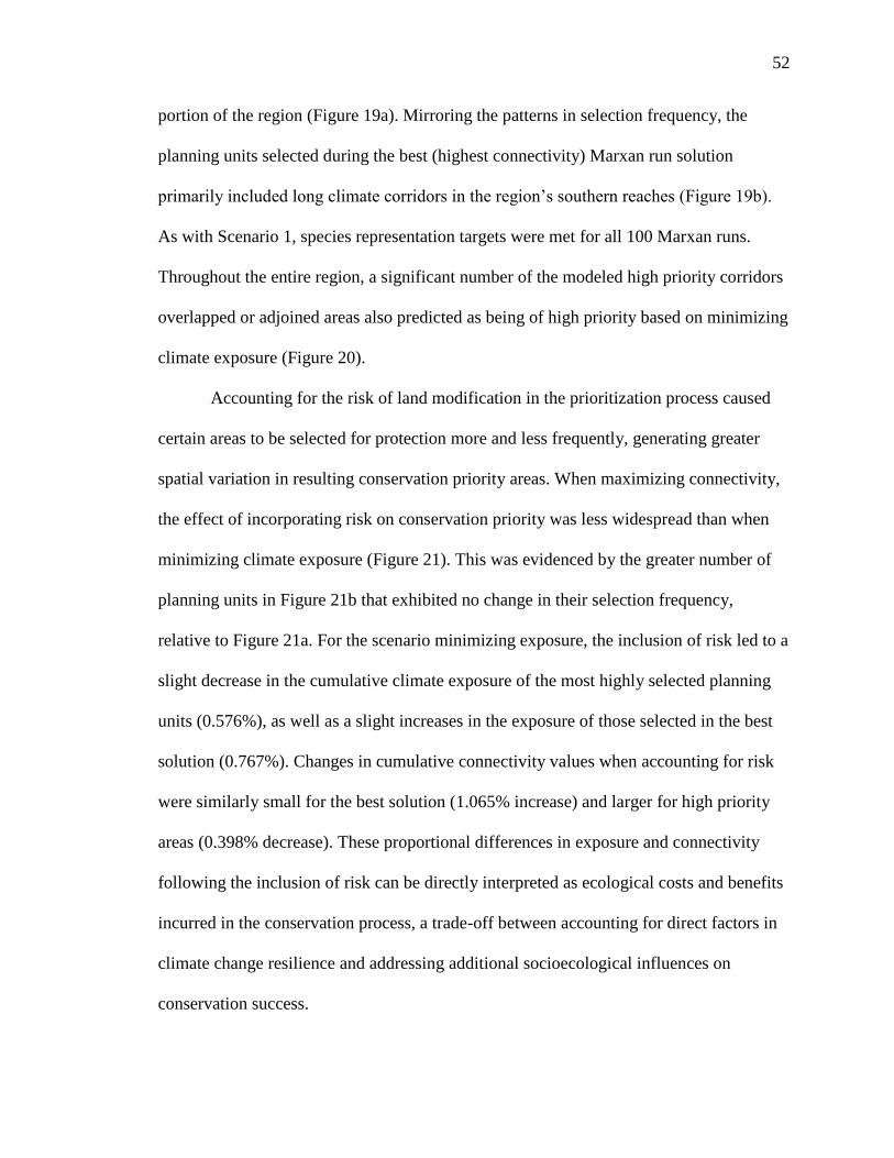
52

portion of the region (Figure 19a). Mirroring the patterns in selection frequency, the

planning units selected during the best (highest connectivity) Marxan run solution

primarily included long climate corridors in the region’s southern reaches (Figure 19b).

As with Scenario 1, species representation targets were met for all 100 Marxan runs.

Throughout the entire region, a significant number of the modeled high priority corridors

overlapped or adjoined areas also predicted as being of high priority based on minimizing

climate exposure (Figure 20).

Accounting for the risk of land modification in the prioritization process caused

certain areas to be selected for protection more and less frequently, generating greater

spatial variation in resulting conservation priority areas. When maximizing connectivity,

the effect of incorporating risk on conservation priority was less widespread than when

minimizing climate exposure (Figure 21). This was evidenced by the greater number of

planning units in Figure 21b that exhibited no change in their selection frequency,

relative to Figure 21a. For the scenario minimizing exposure, the inclusion of risk led to a

slight decrease in the cumulative climate exposure of the most highly selected planning

units (0.576%), as well as a slight increases in the exposure of those selected in the best

solution (0.767%). Changes in cumulative connectivity values when accounting for risk

were similarly small for the best solution (1.065% increase) and larger for high priority

areas (0.398% decrease). These proportional differences in exposure and connectivity

following the inclusion of risk can be directly interpreted as ecological costs and benefits

incurred in the conservation process, a trade-off between accounting for direct factors in

climate change resilience and addressing additional socioecological influences on

conservation success.

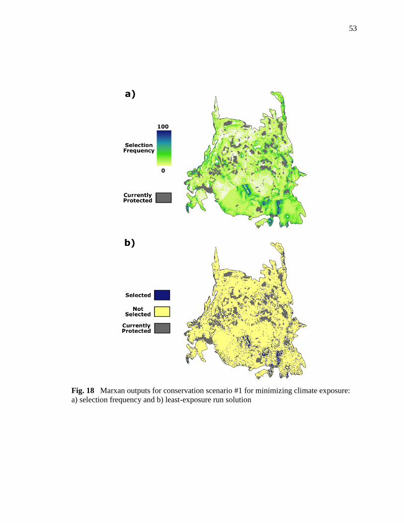
53

Fig. 18 Marxan outputs for conservation scenario #1 for minimizing climate exposure:

a) selection frequency and b) least-exposure run solution

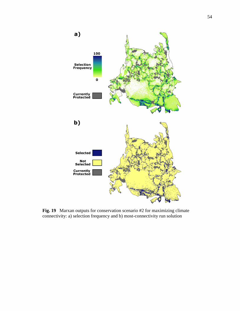
54

Fig. 19 Marxan outputs for conservation scenario #2 for maximizing climate

connectivity: a) selection frequency and b) most-connectivity run solution

55

Fig. 20 Adjoining high priority areas (climate corridors and climate refugia)

By ignoring the current protected area status of the planning units, prioritization

aimed at minimizing climate exposure was used to identify optimal climate refugia and

evaluate the relative resilience of currently protected areas to climate impacts. Only

22.89% of optimal climate refugia (top 5% by selection frequency) fell within currently

protected planning units (Figure 22). These optimal climate refugia overlapped more

widely with the lowest-exposure areas, with 90.98% of refugia area located within an

extent of low exposure areas equivalent in size to the existing protected area network.

Currently protected planning units also varied in their overall climate exposure values

and in their conservation priority following the inclusion of species targets and risk. Both

climate exposure and modeled conservation priority across the entire network of

56

protected planning units was comparable to that across the entire Southern Rockies

region (Figure 23), though mean priorities were higher and mean exposure lower in the

protected areas relative to the broader region. While some contiguous protected areas had

higher exposure and lower priority than the regional averages, many demonstrated the

opposite pattern (Figure 24). Variation in conservation priority within individual

protected areas was considerably greater than variation in exposure.

Fig. 21 Change in conservation priority (selection frequency) when accounting for risk

and ignoring risk in scenarios for a) minimizing climate exposure and b) maximizing

connectivity

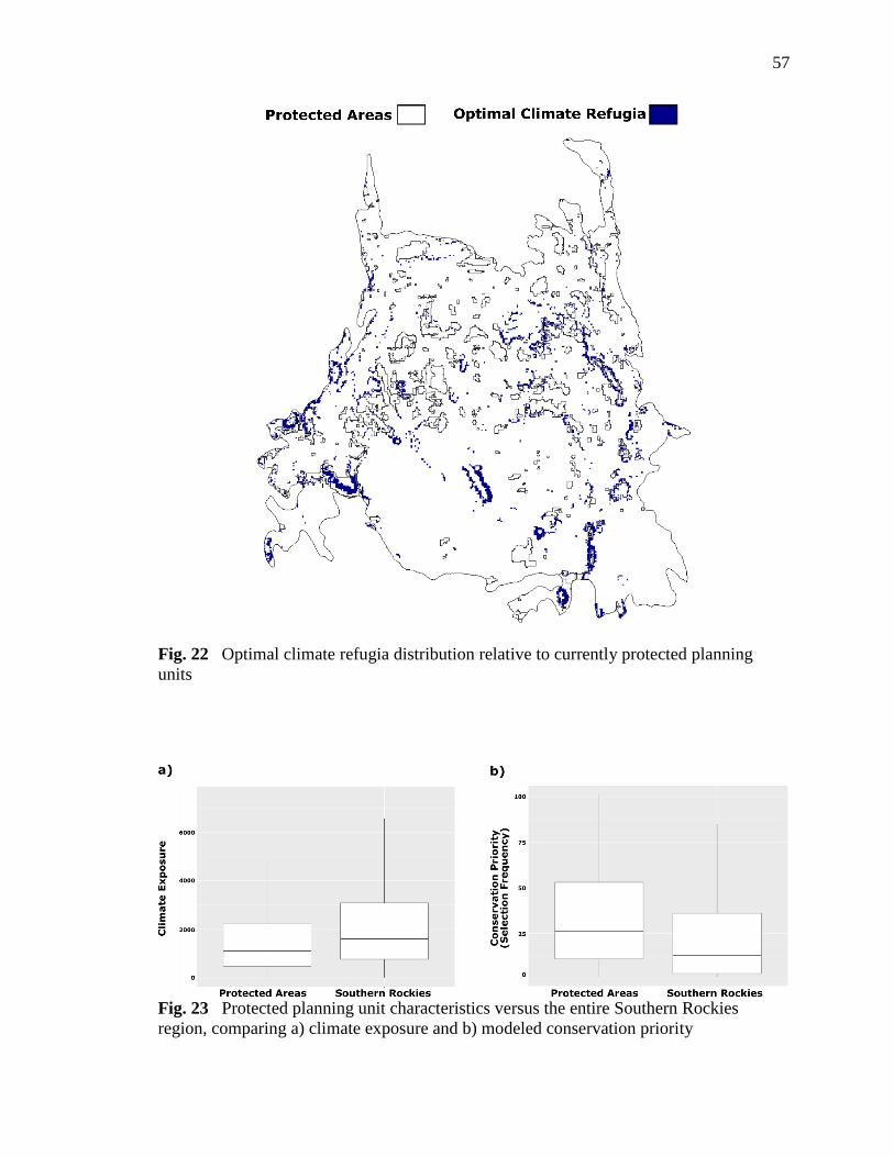
57

Fig. 22 Optimal climate refugia distribution relative to currently protected planning

units

Fig. 23 Protected planning unit characteristics versus the entire Southern Rockies

region, comparing a) climate exposure and b) modeled conservation priority

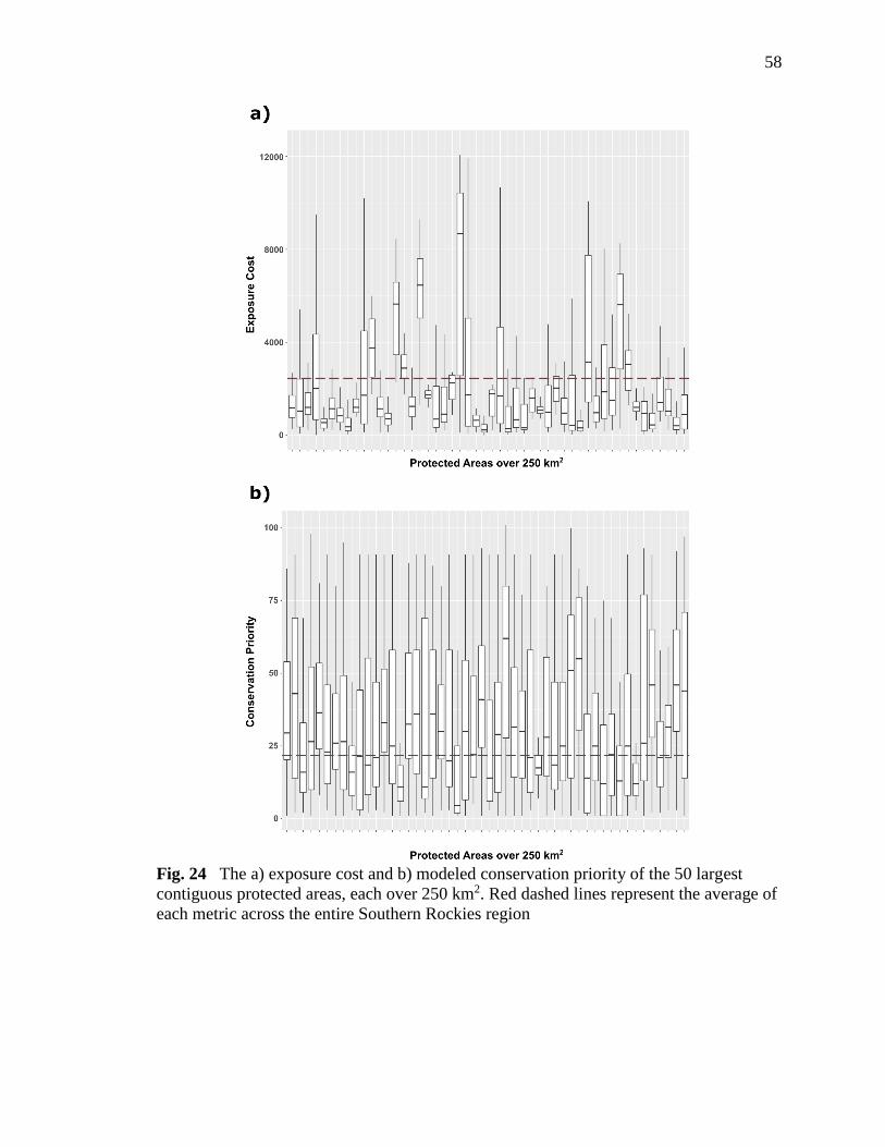
58

Fig. 24 The a) exposure cost and b) modeled conservation priority of the 50 largest

contiguous protected areas, each over 250 km2. Red dashed lines represent the average of

each metric across the entire Southern Rockies region

59

DISCUSSION

Here I have presented a framework for systematically integrating climatic

vulnerabilities into protected area conservation. Not only does this framework allow one

to merge multiple conservation objectives – including threatened species protection and

reduction of climate vulnerabilities – into the planning process, its outcomes are

improved by doing so. Through achieving a balance between multiple species protection

and broader ecological costs, tools such as Marxan can greatly focus one’s management

options towards the areas with the highest potential for positive outcomes.

With the primary aim of building a framework for enhancing the climate

resilience of protected area networks, I modeled conservation priorities in the Southern

Rockies region as a combination of both biotic and abiotic management goals. I identified

potential networks of climate refugia and corridors that simultaneously house species of

concern. Patterns of relative conservation priority across the landscape aligned closely to

the climate resilience metric used in the selection process – exposure or connectivity –

but also reflected the diversity of species targets. Though patterns in priority based on

exposure and connectivity showed little similarity, I was able to further extract areas that

demonstrated high priority across those two contrasting conservation scenarios by

looking at the overlap between the highest climate refugia and corridors.

The methods that I have presented here also provide a means to account for a

wider variety of risks in addition to climate change. As it was not the primary purpose of

this study to predict human responses to climate change, the metric I chose to simulate

the probability of conservation failure (percentage of modified land cover) was relatively

simple and did not account for the full variety of ecological risks within the region, such

60

as oil and gas development (Copeland et al., 2009; Bryce et al., 2012). Importantly,

however, even this spatially-confined stressor still had a clear impact on the distribution

of climate-based conservation priorities, demonstrating both the importance of

accounting for risk and the ability of my framework to do so. Landscape managers

seeking to apply the results of this prioritization framework toward on-the-ground

decision making may be interested more thoroughly evaluating the ecological and social

factors contributing to conservation success in a manner that is most relevant in their

jurisdictions. Despite the direct role that risks can play in this type of conservation

decision making, understanding and quantifying the spatial distributions of future

probabilities of conservation success and failure remains an area of critical research need

(Williamson & Schwartz, 2017).

The existing protected area system of the Southern Rockies has demonstrated

moderate but highly variable levels of vulnerability to climate change. The variability in

exposure and priority between and within areas of current protection suggests that certain

protected areas are projected to experience more or less intense pressures from climate

change. Overall, climate exposure was observably lower in current protected areas than

the average across the region, indicating that they are slightly less vulnerable to climate

shifts due to their greater adaptability. However, the lack of overlap between current

protected areas and optimal climate refugia demonstrated here suggests improvements

that could be made upon the existing protected area system in order to reduce

vulnerability while meeting the set conservation targets.

By concentrating the selection of new protected areas on places where climate

exposure is low and connectivity is high, conservation practitioners could enable species

61

to more effectively shift their distributions in response to novel climate conditions,

allowing broader systems to remain resilient through adaptation and transformation

(Walker et al., 2004; Sayer et al., 2013). Particularly under a changing climate, the

sustainability of any given socioecological system benefits from an understanding of the

system’s limit and barriers to adaptation, as well as explicit acknowledgement of the need

for transformability (Preston et al., 2013). Where ecological shifts due to climate change

are seemingly inevitable, it may be necessary to focus conservation on facilitating those

shifts, aiming the trajectories of the systems toward more desirable states (Folke et al.,

2010; Preston et al., 2013; Hobbs et al., 2014).

62

CHAPTER 4

SUMMARY AND CONCLUSIONS

Efforts must still be made to explicitly account for climate change in conservation

decision making processes (Jones et al., 2016; Reside et al., 2017). However, it remains

uncertain how best to integrate climate change impacts into the ongoing practices of

creating and managing protected landscapes (Game et al., 2011; Hannah et al., 2016).

While past studies have made general management recommendations for buffering

protected ecological resources against climate change impacts, including the conservation

of climate change refugia and landscape corridors, paths toward their actual

implementation have been limited (Hannah et al., 2016; Morelli et al., 2016). Across

broad, diverse regions such as the Southern Rockies and the other areas of the LCC

network, landscape conservation remains driven by pre-existing management needs, such

as protection of individual species of concern (e.g. mule deer, elk) and other focal

resources (e.g. sagebrush steppe ecosystems, cultural landscapes). Furthermore, the

capability to successfully conserve a region’s focal resources depends on many factors

aside from climate change impacts, such as the impacts of human development. Any

efforts to effectively implement one of the recommended strategies for promoting climate

resilience (refugia, corridors, etc.) should incorporate these additional factors to boost

overall effectiveness in the longer term.

In order to make conservation decisions in direct response to climate change,

landscape managers must first understand how climate change vulnerabilities are

spatially and temporally distributed (Dawson et al., 2011). In Chapter 2, I demonstrated

how one can model climate change exposure and connectivity so as to identify areas of

63

the landscape that are generally at the lowest risk of being altered by climate shifts. Since

these metrics of exposure and connectivity are often based entirely on individual climate

variables, they do inevitably ignore the multitude of biotic and abiotic landscape

characteristics that contribute to the individual vulnerabilities of species and ecosystems

to climate change, including edaphic, climatic, and anthropogenic conditions (Dawson et

al., 2011). However, protected area management occurs across broad landscapes that

span numerous unique and diverse components. Limitations on time and resources make

it so that the case-by-case vulnerability cannot be thoroughly quantified across all those

components. At the same time, the gathering of additional information through

assessment and monitoring does not necessarily improve conservation outcomes

(McDonald-Madden et al., 2010). This suggests that it would be prudent to move forward

with climate-based decision making using coarse-filter vulnerability assessments,

especially where individualized assessments are lacking. What generalized metrics of

exposure and connectivity lack in specificity, they make up for in their broad

applicability and adaptability. By quantifying climate vulnerability across one’s multiple

systems using only the few variables that are most broadly and ecologically meaningful,

one could rapidly and cost-effectively propose conservation of various combinations of

resources within the region. Recommendations produced by this broad approach could

then act as a starting point, from which managers could tailor their treatment of

vulnerability in a way the best fits regional conservation goals.

As a second step for improving climate-driven conservation outcomes, landscape

managers can improve upon existing protected area networks by adaptively combining

generalized metrics of climate change vulnerability with the distributions of their

64

conservation targets. In Chapter 3, I showed how one can identify priority areas for

conserving ecological features of the landscape under various scenarios aimed at

protecting either climate refugia or landscape corridors. I demonstrated how priorities can

shift as a result of changing one’s primary conservation objective (e.g. minimizing

exposure vs. maximizing connectivity), accounting for risks to conservation success (e.g.

anthropogenic land modification), and including existing protected areas. In the process, I

assessed the potential resilience of existing protected areas by evaluating their relative

climate exposure and their overlap with optimized climate refugia. Importantly, this

research was mainly aimed at prioritizing where to undergo certain conservation actions,

a significant but small piece of a much broader conservation puzzle. As with any

individual decision support framework, the spatial prioritization methods that I have

described would best be utilized in combination with complementary frameworks that are

better suited for answering the other key conservation questions, such as how to conserve

the resources in the high priority areas (Schwartz et al., 2017). For instance, spatial

conservation tools can provide means for identifying climate refugia, but other decisions

must be made in which specific management actions to take (e.g. restoration, habitat

protection, assisted migration). Addressing the various issues and challenges confronted

in conservation decision making requires a holistic set of decision making approaches

that explicitly acknowledge project purposes and limitations (Game et al., 2013;

Schwartz et al., 2017).

In order to move forward with conservation activities that explicitly and

systematically account for the impacts of climate change, further research is necessary in

a few key areas. Firstly, while the research I have outlined builds on existing decision

65

support frameworks by prioritizing landscape conservation based on assessed

vulnerabilities and multiple conservation targets, improvements to model inputs would

greatly enhance the robustness and real-world applicability of such frameworks. Each

model of climate exposure, connectivity, and conservation priority comes with limitations

in data availability and suitability, such as the lack of comprehensive fine-scale climate

data needed for widely identifying climate microrefugia (Ashcroft, 2010; Morelli et al.,

2016). Secondly, there is an increasing recognition of the need to account for indirect

effects on the likelihood of conservation success, particularly those associated with

human responses to climate change (Game et al., 2013; Chapman et al., 2014; Jones et

al., 2016). For instance, changes in patterns of precipitation could partially drive patterns

in human development, promoting land uses that degrade habitats currently available for

conservation (Faleiro et al., 2013). Despite the risk that indirect effects pose to

conservation, spatial quantification of the factors contributing to conservation action

success is an area in need of greater exploration. Finally, further efforts to aid in climate-

based conservation must be made to better integrate with existing landscape management

contexts, as efficient conservation depends on making use of minimal resources to yield

maximum returns on management investments (Bottrill et al., 2008; Game et al., 2013;

Schwartz et al., 2017). Through more direct collaboration with landscape managers and

stakeholders within the study region, conservation problems and challenges become more

clearly defined, ideally resulting in decision support frameworks that are best suited to

the stakeholders, and to the landscapes under consideration.

66

REFERENCES

Ashcroft MB (2010) Identifying refugia from climate change. Journal of Biogeography, 37,

1407–1413.

Ayram CAC, Mendoza ME, Etter A, Salicrup DRP (2016) Habitat connectivity in biodiversity

conservation: A review of recent studies and applications. Progress in Physical Geography,

40, 7–37.

Ball IR, Possingham HP, Watts ME (2009) Marxan and Relatives: Spatial Conservation

Prioritization. In: Spatial Conservation Prioritization: Quantitative methods and

Computational Tools (eds Moilanen A, Wilson KA, Possingham HP), pp. 185–195. Oxford

University Press, Oxford, United Kingdom.

Ban NC, Pressey RL, Weeks S (2012) Conservation Objectives and Sea-Surface Temperature

Anomalies in the Great Barrier Reef. Conservation Biology, 26, 799–809.

Beier P (2012) Conceptualizing and designing corridors for climate change. Ecological

Restoration, 30, 312–319.

Betts MG, Villard M-A (2009) Landscape thresholds in species occurence as quantitative targets

in forest management: generality in space and time? In: Setting Conservation Targets for

Managed Forest Landscapes (eds Villard M-A, Jonsson BG), pp. 185–206. Cambridge

University Press, Cambridge, United Kingdom.

BirdLife International and Handbook of the Birds of the World (2016) Bird species distribution

maps of the world. Version 6.0 [vector digital data].

Bottrill MC, Joseph LN, Carwardine J et al. (2008) Is conservation triage just smart decision

making? Trends in Ecology and Evolution, 23, 649–654.

Brown JH, Valone TJ, Curtin CG (1997) Reorganization of an Arid Ecosystem in Response to

Recent Climate Change. Proceedings of the National Academy of Sciences, 94, 9729–9733.

Bryce SA, Strittholt JR, Ward BC, Bachelet DM (2012) Colorado Plateau Rapid Ecoregional

67

Assessment Report. Denver, Colorado, United States.

Burrows MT, Schoeman DS, Buckley LB et al. (2011) The pace of shifting climate in marine and

terrestrial ecosystems. Science, 334, 652–655.

Burrows MT, Schoeman DS, Richardson AJ et al. (2014) Geographical limits to species-range

shifts are suggested by climate velocity. Nature, 507, 492–5.

Carroll C, Lawler JJ, Roberts DR, Hamann A (2015) Biotic and climatic velocity identify

contrasting areas of vulnerability to climate change. PLoS ONE, 10.

Carroll C, Wang T, Roberts DR et al. (2017) Scale-dependent complementarity of climatic

velocity and environmental diversity for identifying priority areas for conservation under

climate change. 4508–4520.

CBD (2016a) Decision adopted by the Conference of the Parties to the Convention on Biological

Diversity at its Thirteenth Meeting. Decision XIII/2. Progress towards the achievement of

Aichi Biodiversity Targets 11 and 12. , pp. 1–4. Secretariat for the Convention on

Biological Diversity, Cancun, Mexico.

CBD (2016b) Decision adopted by the Conference of the Parties to the Convention on Biological

Diversity at its Thirteenth Meeting. Decision XIII/4. Biodiversity and climate change. , pp.

1–5. Secretariat for the Convention on Biological Diversity, Cancun, Mexico.

Chapin FS, Kofinas GP, Folke C (2009) Principles of Ecosystem Stewardship: Resilience-Based

Natural Resource Management in a Changing World. 1-409 pp.

Chapman S, Mustin K, Renwick AR, Segan DB, Hole DG, Pearson RG, Watson JEM (2014)

Publishing trends on climate change vulnerability in the conservation literature reveal a

predominant focus on direct impacts and long time-scales. Diversity and Distributions, 20,

1221–1228.

Chen I-C, Hill JK, Ohlemuller R, Roy DB, Thomas CD (2011) Rapid Range Shifts of Species

Associated with High Levels of Climate Warming. Science, 333, 1024–1026.

Copeland HE, Doherty KE, Naugle DE, Pocewicz A, Kiesecker JM (2009) Mapping Oil and Gas

68

Development Potential in the US Intermountain West and Estimating Impacts to Species.

PLoS ONE, 4, 1–7.

Corlett RT, Westcott DA (2013) Will plant movements keep up with climate change? Trends in

Ecology and Evolution, 28, 482–488.

Dawson TP, Jackson ST, House JI, Prentice IC, Mace GM (2011) Beyond Predictions:

Biodiversity Conservation in a Changing Climate. Science, 332, 53–58.

Dobrowski SZ, Abatzoglou J, Swanson AK, Greenberg JA, Mynsberge AR, Holden ZA,

Schwartz MK (2013) The climate velocity of the contiguous United States during the 20th

century. Global Change Biology, 19, 241–251.

Faleiro F V., Machado RB, Loyola RD (2013) Defining spatial conservation priorities in the face

of land-use and climate change. Biological Conservation, 158, 248–257.

Flato G, Marotzke J, Abiodun B et al. (2013) Evaluation of Climate Models. Climate Change

2013: The Physical Science Basis. Contribution of Working Group I to the Fifth Assessment

Report of the Intergovernmental Panel on Climate Change, 741–866.

Folke C, Carpenter SR, Walker B, Scheffer M, Chapin T, Rockström J (2010) Resilience

thinking: Integrating resilience, adaptability and transformability. Ecology and Society, 15.

Fuller RA, McDonald-Madden E, Wilson KA et al. (2010) Replacing underperforming protected

areas achieves better conservation outcomes. Nature, 466, 365–367.

Game ET, Lipsett-Moore G, Saxon E, Peterson N, Sheppard S (2011) Incorporating climate

change adaptation into national conservation assessments. Global Change Biology, 17,

3150–3160.

Game ET, Kareiva P, Possingham HP (2013) Six Common Mistakes in Conservation Priority

Setting. Conservation Biology, 27, 480–485.

Gonzalez P, Neilson RP, Lenihan JM, Drapek RJ (2010) Global patterns in the vulnerability of

ecosystems to vegetation shifts due to climate change. Global Ecology and Biogeography,

19, 755–768.

69

Hamann A, Roberts DR, Barber QE, Carroll C, Nielsen SE (2015) Velocity of climate change

algorithms for guiding conservation and management. Global Change Biology.

Hannah L (2011) Climate Change, Connectivity, and Conservation Success. Conservation

Biology, 25, 1139–1142.

Hannah L, Midgley GF, Lovejoy T et al. (2002a) Conservation of Biodiversity in a Changing

Climate. Conservation Biology, 16, 264–268.

Hannah L, Midgley GF, Millar D (2002b) Climate change-integrated conservation strategies.

Global Ecology and Biogeography, 11, 485–495.

Hannah L, Midgley G, Andelman S et al. (2016) Protected Area Needs in a Changing Climate.

Frontiers in Ecology and the Environment, 5, 131–138.

Harsch MA, Hulme PE, McGlone MS, Duncan RP (2009) Are treelines advancing? A global

meta-analysis of treeline response to climate warming. Ecology Letters, 12, 1040–1049.

Hawkins E, Sutton R (2009) The potential to narrow uncertainty in regional climate predictions.

Bulletin of the American Meteorological Society, 90, 1095–1107.

Heller NE, Zavaleta ES (2008) Biodiversity management in the face of climate change: A review

of 22 years of recommendations. Biological Conservation, 142, 14–32.

Hobbs RJ, Higgs E, Hall CM et al. (2014) Managing the whole landscape: Historical, hybrid, and

novel ecosystems. Frontiers in Ecology and the Environment, 12, 557–564.

Holling CS (1973) Resilience and Stability of Ecological Systems. Annual Review of Ecology and

Systematics, 4, 1–23.

Homer CG, Dewitz JA, Yang L et al. (2015) Completion of the 2011 National Land Cover

Database for the conterminous United States-Representing a decade of land cover change

information. Photogrammetric Engineering and Remote Sensing, 81, 345–354.

IPCC (2014) Climate Change 2014: Synthesis Report. Contribution of Working Groups I, II and

III to the Fifth Assessment Report of the Intergovernmental Panel on Climate Change (eds

Core Writing Team, Pachauri RK, Meyer LA). IPCC, Geneva, Switzerland, 151 pp.

70

IUCN (2016) The IUCN Red List of Threatened Species Version 2016-3.

Jones PD, Kelly PM (1983) The spatial and temporal characteristics of Northern Hemisphere

surface air temperature variations. Journal of Climatology, 3, 243–252.

Jones KR, Watson JEM, Possingham HP, Klein CJ (2016) Incorporating climate change into

spatial conservation prioritisation: A review. Biological Conservation, 194, 121–130.

Kavanagh DM, Nuñez TA, McRae BH (2012) Climate Linkage Mapper Connectivity Analysis

Software.

Koenig WD (2002) Global Patterns of Environmental Synchrony and the Moran Effect.

Ecography, 25, 283–288.

Lacher I, Wilkerson ML (2013) Wildlife Connectivity Approaches and Best Practices in U.S.

State Wildlife Action Plans. Conservation Biology, 28, 13–21.

Landscape Conservation Cooperatives (2014) LCC Network Strategic Plan 2014.

Lawler JJ (2009) Climate Change Adaptation Strategies for Resource Management and

Conservation Planning. Annals of the New York Academy of Sciences, 1162, 79–98.

Levy JS, Ban NC (2013) A method for incorporating climate change modelling into marine

conservation planning: An Indo-west Pacific example. Marine Policy, 38, 16–24.

Loarie SR, Duffy PB, Hamilton H, Asner GP, Field CB, Ackerly DD (2009) The velocity of

climate change. Nature, 462, 1052–1055.

Marris E (2011) The End of the Wild. Nature, 469, 7–10.

McDonald-Madden E, Baxter PWJ, Fuller RA, Martin TG, Game ET, Montambault J,

Possingham HP (2010) Monitoring does not always count. Trends in Ecology and

Evolution, 25, 547–550.

McRae BH, Kavanagh DM (2011) Linkage Mapper Connectivity Analysis Software.

Morelli TL, Daly C, Dobrowski SZ et al. (2016) Managing Climate Change Refugia for Climate

Adaptation. PLoS ONE, 11, 1–17.

Nuñez TA, Lawler JJ, McRae BH et al. (2013) Connectivity Planning to Address Climate

71

Change. Conservation Biology, 27, 407–416.

Oliver TH, Heard MS, Isaac NJB et al. (2015) Biodiversity and Resilience of Ecosystem

Functions. Trends in Ecology & Evolution, 30, 673–684.

Omernik JM, Griffith GE (2014) Ecoregions of the Conterminous United States: Evolution of a

Hierarchical Spatial Framework. Environmental Management, 54, 1249–1266.

Pacifici M, Foden WB, Visconti P et al. (2015) Assessing species vulnerability to climate change.

Nature Climate Change, 5, 215–224.

Parmesan C, Yohe G (2003) A globally coherent fingerprint of climate change impacts across

natural systems. Nature, 421, 37–42.

Pressey RL, Cabeza M, Watts ME, Cowling RM, Wilson KA (2007) Conservation planning in a

changing world. Trends in Ecology and Evolution, 22, 583–592.

Preston BL, Dow K, Berkhout F (2013) The Climate Adaptation Frontier. Sustainability, 5,

1011–1035.

Prugh LR, Hodges KE, Sinclair ARE, Brashares JS (2008) Effect of habitat area and isolation on

fragmented animal populations. Proceedings of the National Academy of Sciences, 105,

20770–20775.

R Core Team (2016) R: A language and environment for statistical computing.

Reside AE, Butt N, Adams VM (2017) Adapting systematic conservation planning for climate

change. Biodiversity and Conservation, 27, 1–29.

Riahi K, Rao S, Krey V et al. (2011) RCP 8.5-A scenario of comparatively high greenhouse gas

emissions. Climatic Change, 109, 33–57.

Sayer J, Sunderland T, Ghazoul J et al. (2013) Ten principles for a landscape approach to

reconciling agriculture, conservation, and other competing land uses. Proceedings of the

National Academy of Sciences, 110, 8349–8356.

Schloss CA, Nuñez TA, Lawler JJ (2012) Dispersal will limit ability of mammals to track climate

change in the Western Hemisphere. Proceedings of the National Academy of Sciences, 109,

72

8606–8611.

Schwartz MW, Cook CN, Pressey RL et al. (2017) Decision Support Frameworks and Tools for

Conservation. Conservation Letters, 00, 1–12.

Settele J, Scholes RJ, Betts RA et al. (2014) Terrestrial and Inland Water Systems. In: Climate

Change 2014: Impacts, Adaptation, and Vulnerability. Part A: Global and Sectoral Aspects.

Contribution of Working Group II to the Fifth Assessment Report of the Intergovernmental

Panel on Climate Change (eds Field CB, Barros VR, Dokken DJ, Mach KJ, Mastrandrea

MD, Bilir TE, Chatterjee M, Ebi KL, Estrada YO, Genova RC, Girma B, Kissel ES, Levy

AN, MacCracken S, Mastrandrea PR, White LL), pp. 271–359. Cambridge University

Press, Cambridge, United Kingdom and New York, NY, USA.

Southern Rockies Landscape Conservation Cooperative (2018) Southern Rockies LCC.

Taylor KE, Stouffer RJ, Meehl GA (2012a) An overview of CMIP5 and the experiment design.

Bulletin of the American Meteorological Society, 93, 485–498.

Taylor PD, Fahrig L, Henein K, Merriam G (2012b) Connectivity is a Vital Element of

Landscape Structure. Oikos, 68, 571–573.

Thomson AM, Calvin K V., Smith SJ et al. (2011) RCP4.5: A pathway for stabilization of

radiative forcing by 2100. Climatic Change, 109, 77–94.

Tischendorf L, Fahrig L (2000a) On the usage and measurement of landscape connectivity.

Oikos, 90, 7–19.

Tischendorf L, Fahrig L (2000b) How should we measure landscape connectivity? Landscape

Ecology, 15, 633–641.

USGS Gap Analysis Program (2016) Protected Areas Database of the United States (PAD-US),

version 1.4 [vector digital data].

Venter O, Fuller RA, Segan DB et al. (2014) Targeting Global Protected Area Expansion for

Imperiled Biodiversity. PLoS Biology, 12, 7.

Walker B, Holling CS, Carpenter SR, Kinzig A (2004) Resilience , Adaptability and

73

Transformability in Social-ecological Systems. Ecology & Society, 9, 5.

Walther GR, Post E, Convey P et al. (2002) Ecological responses to recent climate change.

Nature, 416, 389–395.

Wang T, Hamann A, Spittlehouse D, Carroll C (2016) Locally downscaled and spatially

customizable climate data for historical and future periods for North America. PLoS ONE,

11, 1–11.

Williamson MA, Schwartz MW (2017) Spatially explicit estimates of the likelihood of

conservation action. In: Annual Meeting of the Ecological Society of America. Portland,

Oregon, USA.

Wilson KA, McBride MF, Bode M, Possingham HP (2006) Prioritizing global conservation

efforts. Nature, 440, 337–340.

74

APPENDICES

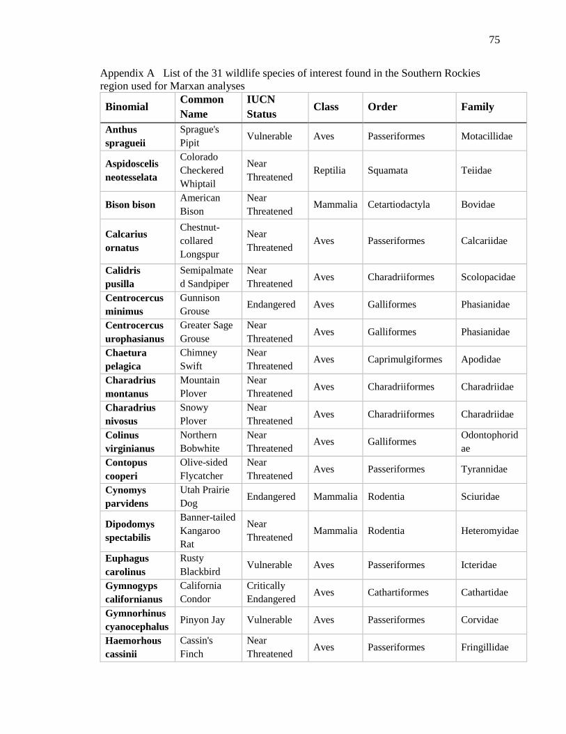
75

Appendix A List of the 31 wildlife species of interest found in the Southern Rockies

region used for Marxan analyses

Binomial Common

Name

IUCN

Status Class Order Family

Anthus

spragueii

Sprague's

Pipit Vulnerable Aves Passeriformes Motacillidae

Aspidoscelis

neotesselata

Colorado

Checkered

Whiptail

Near

Threatened Reptilia Squamata Teiidae

Bison bison American

Bison

Near

Threatened Mammalia Cetartiodactyla Bovidae

Calcarius

ornatus

Chestnut-

collared

Longspur

Near

Threatened Aves Passeriformes Calcariidae

Calidris

pusilla

Semipalmate

d Sandpiper

Near

Threatened Aves Charadriiformes Scolopacidae

Centrocercus

minimus

Gunnison

Grouse Endangered Aves Galliformes Phasianidae

Centrocercus

urophasianus

Greater Sage

Grouse

Near

Threatened Aves Galliformes Phasianidae

Chaetura

pelagica

Chimney

Swift

Near

Threatened Aves Caprimulgiformes Apodidae

Charadrius

montanus

Mountain

Plover

Near

Threatened Aves Charadriiformes Charadriidae

Charadrius

nivosus

Snowy

Plover

Near

Threatened Aves Charadriiformes Charadriidae

Colinus

virginianus

Northern

Bobwhite

Near

Threatened Aves Galliformes

Odontophorid

ae

Contopus

cooperi

Olive-sided

Flycatcher

Near

Threatened Aves Passeriformes Tyrannidae

Cynomys

parvidens

Utah Prairie

Dog Endangered Mammalia Rodentia Sciuridae

Dipodomys

spectabilis

Banner-tailed

Kangaroo

Rat

Near

Threatened Mammalia Rodentia Heteromyidae

Euphagus

carolinus

Rusty

Blackbird Vulnerable Aves Passeriformes Icteridae

Gymnogyps

californianus

California

Condor

Critically

Endangered Aves Cathartiformes Cathartidae

Gymnorhinus

cyanocephalus Pinyon Jay Vulnerable Aves Passeriformes Corvidae

Haemorhous

cassinii

Cassin's

Finch

Near

Threatened Aves Passeriformes Fringillidae

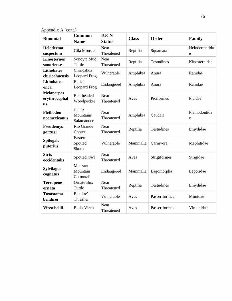
76

Appendix A (cont.)

Binomial Common

Name

IUCN

Status Class Order Family

Heloderma

suspectum Gila Monster

Near

Threatened Reptilia Squamata

Helodermatida

e

Kinosternon

sonoriense

Sonoyta Mud

Turtle

Near

Threatened Reptilia Testudines Kinosternidae

Lithobates

chiricahuensis

Chiricahua

Leopard Frog Vulnerable Amphibia Anura Ranidae

Lithobates

onca

Relict

Leopard Frog Endangered Amphibia Anura Ranidae

Melanerpes

erythrocephal

us

Red-headed

Woodpecker

Near

Threatened Aves Piciformes Picidae

Plethodon

neomexicanus

Jemez

Mountains

Salamander

Near

Threatened Amphibia Caudata

Plethodontida

e

Pseudemys

gorzugi

Rio Grande

Cooter

Near

Threatened Reptilia Testudines Emydidae

Spilogale

putorius

Eastern

Spotted

Skunk

Vulnerable Mammalia Carnivora Mephitidae

Strix

occidentalis Spotted Owl

Near

Threatened Aves Strigiformes Strigidae

Sylvilagus

cognatus

Manzano

Mountain

Cottontail

Endangered Mammalia Lagomorpha Leporidae

Terrapene

ornata

Ornate Box

Turtle

Near

Threatened Reptilia Testudines Emydidae

Toxostoma

bendirei

Bendire's

Thrasher Vulnerable Aves Passeriformes Mimidae

Vireo bellii Bell's Vireo Near

Threatened Aves Passeriformes Vireonidae