Theoretical and Mathematical Physics, 178(2): 143–193 (2014)

LANDAU–LIFSHITZ EQUATION, UNIAXIAL ANISOTROPY CASE:

THEORY OF EXACT SOLUTIONS

R. F. Bikbaev,∗ A. I. Bobenko,† and A. R. Its‡

Using the inverse scattering method, we study the XXZ Landau–Lifshitz equation well-known in the theory

of ferromagnetism. We construct all elementary soliton-type excitations and study their interaction. We

also obtain finite-gap solutions (in terms of theta functions) and select the real solutions among them.

Keywords: multisoliton solution, ferromagnetism, finite-gap integration, theta function

1. Introduction

The Landau–Lifshitz (LL) equation [1]

�St = [�S × �Sxx] + [�S × J �S],

�S = (S1, S2, S3), S21 + S2

2 + S23 = 1, J = diag(J1, J2, J3),

(1.1)

well-known in the theory of ferromagnetism, is an object of increased attention from specialists in theoryof completely integrable nonlinear evolutionary systems. This specific interest in Eq. (1.1), compared withother models embedded in the inverse scattering method, is explained, in particular, by the following fact.The representation of the LL equation as the compatibility condition of two linear equations (a U–V pairrepresentation) was obtained long ago: for the completely isotropic case (J1 = J2 = J3, XXX model)by Takhtajan in 1977 [2], for the uniaxial anisotropy case (J1 = J2 �= J3, XXZ model) by Borovik in1978 [3], and finally for the completely anisotropic case (J1 �= J2 �= J3, XYZ model) by Sklyanin andindependently by Borovik in 1979 (see [4]). It would therefore seem that for Eq. (1.1), we have a possibilityof directly applying the traditional apparatus of the inverse scattering method with all its basic attributes:constructing explicit solutions, studying the Cauchy problem, and so on. But this possibility was notcompletely realized up to the mid-1980s. The difficulty in applying the inverse scattering method to the LLequation is explained by the fact that the LL equation (more than any other integrable system) requiresreformulating the inverse scattering method into the “matrix Riemann problem method,” which was notyet completely realized when the U–V pair was written for Eq. (1.1), although reformulating the inversescattering method in this direction, strictly speaking, had already begun in 1975 in the well-known papersby Shabat, Zakharov, and Manakov [5], [6].

∗Deceased.†St. Petersburg Department of the Steklov Institute of Mathematics, RAS, St. Petersburg, Russia; Institut fur

Mathematik, Technische Universitat Berlin, Berlin, Germany, e-mail: bobenko@math.tu-berlin.de.‡Department of Mathematical Sciences, Indiana University-Purdue University Indianapolis, Indianapolis, In-

diana, USA, e-mail: itsa@math.iupui.edu.

This paper is a revision at the request of the Editorial Board of Preprint No. DonFTI-84-6(81) with the same name,Donetsk Physico-Technical Institute, Academy of Sciences of the Ukrainian SSR, Donetsk, 1984.

Translated from Teoreticheskaya i Matematicheskaya Fizika, Vol. 178, No. 2, pp. 163–219, February, 2014.

Original article submitted March 7, 2013.

0040-5779/14/1782-0143 c© 2014 Springer Science+Business Media, Inc. 143

Thus, starting from 1979, a quite strange situation appeared in the mathematical theory of the LLequation. This equation seemed to be embedded into the scheme of the inverse scattering method, butthere was no real advantage from that. We note that Eq. (1.1) is extremely important from the physicalstandpoint. Therefore, the theory of the LL equation was intensively and quite successfully developingindependently of the “interrelations” with the inverse scattering method. In particular, many specificsolutions of it, both solitons and more complicated types, were known by 1979. In this regard, first ofall, we should mention the papers by Akhiezer and Borovik [7], [8] and the research of Kosevich’s group(Kosevich, Ivanov, Kovalev, Bogdan, Babich, and others) and Eleonskii’s group (Eleonskii, Kirova, Kulagin,and others). We allow ourself to not present numerous citations of these authors, referring the reader tothe review by Kosevich [9] for these citations as well as for a more detailed history of this problem.

Among the papers that used the inverse scattering method as much as was possible in the describedperiod, in addition to the already mentioned papers by Takhtajan, Sklyanin, and Borovik, we note theworks on the finite-gap integration of the LL equation by Bogoljubov Jr. and Prikarpatskii [10] (XXZcase), Cherednik [11], and Date, Jimbo, Koshivara, and Miwa [12] (XYZ case). We also relate the veryinteresting paper by Bogdan and Kovalev [13] (where the N -soliton solutions of the LL equation in thecompletely anisotropic case were constructed by the Hirota method) to this cycle of papers, although theauthors themselves set the Hirota method in opposition to the inverse scattering method (in our view,unjustifiedly).

The fundamental contribution to the development of effective schemes for applying the inverse scat-tering method to the LL equation was made in 1982 after Mikhailov had rigorously defined the matrixRiemann problem with axiomatics suitable to the U–V -pair for the XYZ case of the LL equation in [14].The result appeared immediately: the multisoliton solutions of Eq. (1.1) in the completely anisotropic casewere systematically described by Mikhailov in [14] and by Rodin in [15], while Bobenko [16] and Borisov [17]proposed “dressing procedures” for this equation that allowed constructing new solutions using known ones.There was also progress in the algebraic-geometric (finite-gap) integration of Eq. (1.1): we succeeded inembedding the XXZ case of Eq. (1.1) into Krichever’s scheme and reduced the finite-gap integration ofthis equation to explicit formulas in terms of theta functions [18], and we also implemented an analogousprogram for the completely anisotropic case, thus making the corresponding results in [10] and [11] moreuseful. Summarizing the above discussion, we can state that there is now a scheme in the theory of LLequation (1.1) that allows systematically constructing all previously known solutions, obtaining new exactsolutions essentially different from those already known, and studying various effects associated with theirinteractions.

Our goal here is to present a detailed description of the considered scheme using the intermediateexample (in complexity) of the LL equation in the uniaxial anisotropy case. This paper is intended forspecialists in the ferromagnetism theory and does not assume that the reader has a deep familiarity withthe ideas of the inverse scattering method. We try to give as much attention as possible to concrete results,to physically interesting particular cases, and to the effects obtainable from the approach we have developed.This purpose essentially determines the structure of this paper.

We present the foundation of the scheme in Secs. 2 and 3, formulating and discussing the “generalizedmatrix Riemann problem” corresponding to the XYZ case of the LL equation. Although we start with [14]mentioned above, we nevertheless use a nonstandard version of the transformation of the integrable equationinto the Riemann problem, taking the version from papers by Jimbo, Miwa, and Ueno [19], [20]. It seemsthe most suitable foundation for developing all the basic constructions of our scheme in the subsequentsections. The mathematical apparatus in Secs. 2 and 3 is quite elementary: we use only the simplest ideasof linear algebra and complex analysis (the algebra of 2×2 matrices and the Liouville theorem).

In Secs. 4–6, staying within the framework of this apparatus, we develop the dressing procedure for

144

the XXZ LL equation together with its use to construct, classify, and describe soliton solution interactions.We emphasize that we, apparently, do not obtain new results here. But our derived formulas have manymethodological advantages compared with known representations of the exact solutions of LL equation. Inparticular, all the obtained answers are completely symmetric with respect to the components of the vector�S from the standpoint of the degree of explicitness and compactness. Our formulas are parameterized bypoints of the complex plane (by the spectrum of the appropriate linear problem), which satisfy quite weakconstraints (see Sec. 5). This allows studying various limits in our constructed solutions effectively.

In Sec. 6, we demonstrate the possibilities of our method by describing the effects of mutual inter-actions among different elementary solutions. Here, in addition to rather simple processes of two-solitoninteractions, we also describe the phenomenon of a soliton passing through a domain wall.

We consider essentially new types of solutions of the XXZ LL equation in Secs. 7–10, where we presenta realization of the basic conceptual theorem in Sec. 2 in the framework of the “finite-gap integration”technique based on the already less trivial mathematical apparatus of the theory of functions on compactRiemann surfaces. Unfortunately, we cannot keep the exposition closed here. But we try to minimize theneed to refer to external mathematical sources. The closest source is [21]. The reader can also refer tothe concluding chapters in [22] and the introductory part in [23]. We present supplementary informationon reductions of Riemann surfaces (used in Sec. 9) in the appendix. A more detailed presentation of thetheory of Riemann theta functions (subject to the rules for integrating nonlinear equations) can be foundin [21] (also see [24]–[26]).

We now briefly describe the content of Secs. 7–10. In Sec. 7, we construct complex almost periodic(finite-gap) solutions of the LL equation in the case of uniaxial anisotropy in terms of multidimensionaltheta functions. In Sec. 8, we derive the reality conditions using the technique in [27]. From the standpointof physical applications, the multidimensional theta function is a very complicated object for quantitativeanalysis. But there are currently program packages for calculations on Riemann surfaces [28]. In particular,they allow calculating solutions effectively in terms of theta functions. The multidimensional formulascontaining theta functions hence become valuable for numerical analysis. Moreover, the general expressionsin terms of theta functions are a convenient analytic basis for deriving important particular solutions.

In Sec. 9, we deduce periodic solutions described in terms of elliptic functions (cnoidal waves and theirsuperpositions) from the general formulas in Secs. 7 and 8 using the technique for reducing theta functionsof higher ranks to lower ones. In Secs. 10 and 11, we subject the general formula in Sec. 7 to a certaindegeneration procedure (we pairwise merge the branch points of the original Riemann surface), resultingin convenient formulas for multisoliton solutions and solutions describing the interactions between solitonsand cnoidal waves. More precisely, restricting ourself to the case of the “easy plane” anisotropy for brevity,we construct multisoliton formulas for the solutions of the “moving domain wall” type and describe theinteraction effect between a single moving domain wall and a cnoidal wave.

Summarizing our description of this paper, we note the following. We hope to demonstrate that thedeveloped scheme based on the inverse scattering method is the most appropriate technique for constructing,classifying, and studying exact solutions of the LL equation.

We dedicate this publication to our friend Ramil Faritonovich Bikbaev, untimely deceased.

2. Basic theorem

The XXZ LL equation (J1 = J2, and we take J = diag(0, 0, ε) without loss of generality)

�St = [�S × �Sxx] + [�S × J �S] (2.1)

is the compatibility conditionUt − Vx + [U, V ] = 0 (2.2)

145

for the pair of linear differential equations

Ψx = UΨ, Ψt = V Ψ, (2.3)

where U and V are given by the expressions

U(λ) = −i3∑

α=1

Sαwασα,

V (λ) = 2i

3∑

α=1

Sαw1w2w3w−1α σα − i

3∑

α=1

[S × Sx]αwασα,

(2.4)

w1 = w2 =√

λ2 − a2, w3 = λ, a = i

√ε

4. (2.5)

If ε > 0, then we have anisotropy of the easy magnetization axis type. If ε < 0, then we haveanisotropy of the easy magnetization plane type. Both cases can be studied quite similarly. Pair (2.4) is asimple degeneration of the U–V Sklyanin–Borovik pair for the XYZ LL equation if J1 = J2. We note thatthe spectral parameter λ in the considered case ranges the two-sheet Riemann surface Γ of the function√

λ2 − a2 instead of the complex plane. Of course, we might introduce an appropriate change of the variableλ such that U and V become rational functions of the spectral parameter. But we do not do this, becausein the selected uniformization (2.5) of the relations w2

α − w2β = −(Jα − Jβ)/4, the following reduction of

pair (2.4) can be taken into account very naturally:

σ3U(λτ )σ3 = U(λ), σ3V (λτ )σ3 = V (λ), (2.6)

where λ → λτ denotes the involution transposing the sheets of Γ and√

(λτ )2 − a2 = −√

λ2 − a2. Thisreduction (associated with the transposition of the sheets) can be easily taken into account in constructingfinite-gap solutions (see Sec. 7).

The principal object in constructing exact formulas for solutions of the nonlinear equations integrableby the inverse scattering method is the function Ψ. Precisely this function is first constructed using itsanalytic properties following from the form of U–V -pair. The formulas for solutions of the nonlinearequations can then be constructed using this function. We formulate the so-called generalized Riemannproblem corresponding to Eq. (2.1).

Reimann problem. We must find a function Ψ(λ) defined on Γ, taking values in the set of 2×2matrices, and having the following properties:

1. Two infinitely remote points ∞1,2 of the surface Γ in its standard realization by the two-sheet coveringof the plane of the variable λ (

√λ2 − a2 → ±λ at λ → ∞1,2) are the essential singularity points of Ψ,

which in the neighborhood of these points has an essential singularity differentiable in x and t of theform

Ψ(λ, x, t) =∞∑

j=0

Φj(x, t)λ−je−iσ3λx+2iσ3λ2tCλm, (2.7)

where detΦ0(x, t) �= 0 and the matrix C is invertible and independent of x and t.

2. The function Ψ(λ) also has so-called regular singularities at the points a1, . . . , aN , i.e., Ψ(λ) is holo-morphic and invertible at all points of the set Γ \ {∞1,2}, except the points a1, . . . , aN , independentof x and t, in a neighborhood of which we have the representation

Ψ(λ) =λ∼aj

ΨkTj Cj , j = 1, . . . , N, (2.8)

146

where Tj are diagonal constant matrices and Cj are invertible constant matrices (independent of x

and t). The matrix-valued function Ψ(λ) is holomorphic and invertible in a neighborhood of aj , wherek is a local parameter in the neighborhood of aj ,

k =

⎧⎨

⎩λ − aj , aj �= ±a,√

λ ± a, aj = ±a.

We note that if Tj is a rational noninteger matrix, then the function Ψ(λ) is not single-valued onΓ. In this case, the point aj is a branch point of the covering Γ → Γ, and the function Ψ is alreadysingle-valued on this covering surface Γ and, as a function on Γ, is characterized by the property thatin passing around the point aj on Γ in the positive direction, Ψ(λ) is multiplied on the right by amonodromy matrix,

Ψ(λ) → Ψ(λ)Mj , Mj = C−1j e2πiTj Cj . (2.9)

3. Let there exist contours Li ∈ Γ and matrices Gi(λ), i = 1, . . . , M , independent of x and t. Thenthe matrices Ψ+(λ) and Ψ−(λ) (the boundary values of Ψ from different sides of the contour Li) arecoupled by the linear relations along Li,

Ψ−(λ) = Ψ+(λ)Gi(λ)∣∣λ∈Li

. (2.10)

4. The reduction constraintσ3Ψ(λτ ) = Ψ(λ)σ(λ) (2.11)

holds, where σ(λ) is independent of x and t.

5. The normalization conditions

∂

∂xlog Ψ1i(a) =

∂

∂xlog Ψ2k(−a),

∂

∂tlog Ψ1j(a) =

∂

∂tlog Ψ2l(−a)

(2.12)

hold for any i, k, j, and l.

Theorem 1. Let a function Ψ satisfying conditions 1–5 of the Riemann problem be constructed. Then

the logarithmic derivatives ΨxΨ−1 and ΨtΨ−1 have form (2.4) up to the terms proportional to the identity

matrix, where3∑

α=1

Sασα = Φ0σ3Φ−10 , (2.13)

i.e., if

Φ0 =

(A B

C D

), (2.14)

then

S1 =CD − AB

AD − BC, S2 = −i

CD + AB

AD − BC, S3 =

AD + BC

AD − BC. (2.15)

The functions Sj(x, t) defined by relations (2.13)–(2.15) satisfy the equality

3∑

α=1

S2α = 1

and form a solution of XXZ LL equation (2.1).

147

Proof. We first note that the logarithmic derivatives ΨxΨ−1 and ΨtΨ−1 are single-valued functionson the surface Γ by virtue of properties (2.8)–(2.10), unlike the function Ψ itself. They have no singularitiesat the points aj ,

ΨxΨ−1 =λ∼aj

ΨxkTj CjC−1j k−Tj Ψ−1 = ΨxΨ−1,

and on the contours Li,(Ψ+)xΨ−1

+ = (Ψ−)xΨ−1−∣∣λ∈Li

.

Therefore, from asymptotic form (2.7) and because of the absence of singularities in the set Γ \ {∞1,2}, wehave the following representations of the logarithmic derivatives ΨxΨ−1 and ΨtΨ−1:

ΨxΨ−1 = λA1 +√

λ2 − a2A2 + A3,

ΨtΨ−1 = λ2B1 + λ√

λ2 − a2B2 + λB3 +√

λ2 − a2B4 + B5,

where Ai and Bi are matrices depending only on x and t with

Tr(A1 + A2) = Tr(B1 + B2) = Tr(B3 + B4) = 0.

Further, it follows from reduction (2.11) that the matrices A1, A3, B1, B3, and B5 are diagonal andthe matrices A2, B2, and B4 are antidiagonal. Hence,

ΨxΨ−1 = −i

3∑

α=1

Sαwασα + A(x, t)σ3 + α(x, t)I,

ΨtΨ−1 = 2i

3∑

α=1

Pαw1w2w3w−1α σα + i

3∑

α=1

Qαwασα + B(x, t)σ3 + β(x, t)I.

It follows from normalization condition (2.12) that A(x, t) = B(x, t) = 0. Substituting asymptotic expan-sion (2.7) in (2.3) and equating terms with like degrees of λ, we finally confirm formula (2.13) and theequalities Pα = Sα and Qα = −[S × Sx]α. The theorem is proved.

Therefore, the function Ψ (and consequently the solution of the XXZ LL equation) is defined by thefollowing data of the generalized Riemann problem (the “scattering data”):

Λ = {a1, . . . , aN , Tj, . . . , TN , C1, . . . , CN , L1, . . . ,LM , G1(λ), . . . , GM (λ)}, (2.16)

where Tj and Cj , j = 1, . . . , N , are defined in (2.8) and λ ∈ Li, i = 1, . . . , M , is the argument of Gi(λ).Further, we find exact expressions for Ψ with some particular data Λ and thus construct solutions ofEq. (2.1).

Remark 1. Let the function Ψ satisfy the reduction

σ2Ψ(λ) = Ψ(λ)M(λ), (2.17)

where the conjugation anti-involution on Γ is naturally given as

(λ,√

λ2 − a2)→(λ,√

λ2 − a2)

and M(λ) is a matrix-valued function independent of x and t. Then the solution of Eq. (2.1) (definedby (2.13)–(2.15)) is real.

148

Remark 2. Let the function Ψ(λ) satisfy conditions (2.7)–(2.12) and define the solution �S(x, t). Thenthe function

Ψγ(λ) =

(γ 0

0 γ−1

)Ψ(λ), γ = const ∈ C, (2.18)

also satisfies a generalized Riemann problem. The corresponding solution �Sγ of Eq. (2.1) differs from �S

(we consider only real solutions, |γ| = 1) by a simple rotation of axes 1 and 2 in the plane of these axes (inthe plane perpendicular to the anisotropy axis 3). Obviously, the solutions �S and �Sγ are equivalent fromthe physical standpoint. Further, the function Ψϕ(λ) = ϕ(x, t)Ψ(λ), where ϕ(x, t) is an arbitrary scalarfunction ofx and t, also satisfies a Riemann problem. The corresponding solutions of Eq. (2.1) coincide:�Sϕ(x, t) = �S(x, t).

Remark 3. There are some a priori constraints on the matrices σ(λ) and M(λ) involved in reductionidentities (2.11) and (2.17). In particular, successively applying two transformations (2.11) to Ψ(λ), weobtain the relation

σ(λ)σ(λτ ) ≡ I. (2.19)

Successively applying two transformations (2.17) to Ψ(λ), we obtain the relation

M(λ)M(λ) ≡ −I. (2.20)

Successively applying transformations (2.11) and (2.17) to Ψ(λ), we obtain the relation

σ(λ)M(λτ ) + M(λ)σ(λ) = 0. (2.21)

3. External field

It is well known that a homogeneous external field directed along the anisotropy axis (axis 3 in our case)does not destroy the integrability of a system. In this section, we construct a generalization of the Riemannproblem associated with Eq. (1.1) and formulated in Sec. 2. The XXZ LL equation with an external fielddirected along the anisotropy axis is embedded into the proposed model.

Theorem 2. Let the function Ψ(λ, x, t) have properties 1–4 of the Riemann problem and satisfy the

normalization condition∂

∂xlog Ψ1i(a) =

∂

∂xlog Ψ2k(−a) + i

∂

∂xf(x, t),

∂

∂tlog Ψ1j(a) =

∂

∂tlog Ψ2l(−a) + i

∂

∂tf(x, t)

(3.1)

for some indices i, j, k, and l. Then the logarithmic derivatives ΨxΨ−1 and ΨtΨ−1 are respectively equal

(up to terms proportional to the identity matrix) to

Uf = U +i

2σ3

∂f

∂x, Vf = V +

i

2σ3

∂f

∂t,

where U and V are matrices (2.4). Zakharov–Shabat equation (2.2) for Uf and Vf leads to the equation

�St = [�S × �Sxx] + [�S × J �S] + [�S × �H] − 2�SxS3∂f

∂x, (3.2)

where

J = diag(

0, 0, ε +(

∂f

∂x

)2), �H =

(0, 0,

∂f

∂t

).

149

A particular case of Eq. (3.2) is physically interesting. It describes the nonlinear dynamics of a ferro-magnet in a homogeneous external magnetic field �H(t) arbitrarily depending on t.

Corollary 1. If f(x, t) =∫ t

H(s) ds depends only on t, then this Riemann problem corresponds to

the equation�St = [�S × �Sxx] + [�S × J �S] + [�S × �H ], �H = (0, 0, H(t)). (3.3)

The elementary procedure for constructing solutions of Eq. (3.3) using solutions of Eq. (2.1) followsfrom Corollary 1.

Corollary 2. If s solution �S(x, t) = (S1, S2, S3) of LL equation (2.1) is expressed in terms of A, B, C,

and D using formulas (2.15), then the quantities

Af = A exp(∫ t

H(s) ds

), Bf = B exp

(∫ t

H(s) ds

), Cf = C, Df = D

define the function �Sf (x, t) (which is a solution of Eq. (3.3)) by the same formulas (2.15).

Of course, this purely algebraic fact can be verified directly. Obviously, the solution �Sf is real if �S andH(t) are real.

4. Dressing procedure: General scheme

It is convenient to start this section with the proof of one auxiliary statement [19].

Lemma 1. Let Ψ(λ) be a 2×2 matrix function holomorphic in the neighborhood of the point λ = a,

which is a simple zero of detΨ(λ). Then representation (2.8) holds for the matrix Ψ(λ) in the neighborhood

of the point a with T = ( 1 00 0 ). In this case, any invertible matrix such that the first column of the matrix

C−1 belongs to kerΨ(a) can be taken for C.

Proof. Let C and T be as described in the lemma. The statement in the lemma is equivalent to theholomorphicity and matrix invertibility of the function

Ψ(λ) = Ψ(λ)C−1(λ − a)“−1 0

0 0

”

in some neighborhood of the point a. Let C−1 = (X, Y ). Then (because Ψ(a)X = 0)

Ψ(λ) = Ψ(λ)(X, Y )

((λ − a)−1 0

0 1

)=(

1λ − a

Ψ(λ)X, Ψ(λ)Y)

=

=(

1λ − a

[Ψ(a)X + Ψ′(a)X(λ − a) + · · · ], Ψ(a)Y + (λ − a)Ψ′(a)Y + · · ·)

=

=∞∑

k=0

(λ − a)kΨk,

and the function Ψ(λ) is consequently holomorphic in a neighborhood of a. After the holomorphicity ofΨ(λ) is established, its matrix invertibility follows because the zero of detΨ(λ) at a is simple. The lemmais proved.

150

Now let Ψ0(λ, x, t) be a function satisfying all conditions in Theorem 1 and thus leading to somesolution �S0(x, t) of the LL equation. We let

Λ0 = {a01, . . . , a

0N , T 0

1 , . . . , T 0N , C0

1 , . . . , C0N , L0

1, . . . ,L0N , G0

1(λ), . . . , G0M , m0}

denote the data of the generalized Riemann problem corresponding to Ψ0. Using Ψ0, we want to explicitlyconstruct a new function Ψ(λ, x, t) satisfying the same conditions 1–5 of the Riemann problem but witha new set of data Λ = Λ0 ⊕ Λ′. Hence, having the known solution �S0(x, t) of the LL equation, we wouldconstruct a new solution of it. We seek the function Ψ in the form

Ψ(λ, x, t) = f(λ, x, t)Ψ0(λ, x, t), (4.1)

where f is a 2×2 matrix function meromorphic on Γ and the simple poles at the points ∞1,2 are the onlysingularities. We require that f satisfy the relation

σ3f(λτ )σ3 = f(λ). (4.2)

This equality together with the mentioned conditions for the singularities of f(λ) leads to its representation

f(α) =3∑

α=1

qαwα(α)σα + (q0λ + p0)I + p3σ3, (4.3)

where the scalar functions qα(x, t) and pα(x, t) must still be defined. To determine them, we take the pointsλ1, λ2 /∈ {a0

1, . . . , a0N} ∪ {a,−a} and two complex numbers A1 and A2. Let

Ψ(λj)(

1Aj

)= 0, j = 1, 2, p3 = −aq0. (4.4)

These relations form a linear homogeneous algebraic system of five equations for six unknowns (the qα andpα). Solving this system, we find the sought functions qα(x, t) and pα(x, t) up to a common functionalfactor. Because of Remark 2 at the end of Sec. 1, this freedom is already inessential for us.

Theorem 3. The function Ψ(λ, x, t) defined by formulas (4.1), (4.3), and (4.4) satisfies all conditions

in Theorem 1. The corresponding data of the generalized Riemann problem differ from the original data

Λ0 in the number of regular singular points, which is increased by four,

{a01, . . . , a

0N} → {a0

1, . . . , a0N} ⊕ {λ1, λ2, λ

τ1 , λτ

2},

and by the shift m0 → m0 + I of the matrix m0 by the identity matrix. The corresponding (complex)solution �S(x, t) of the LL equation1 is related to the seed solution �S0(x, t),

S = QS0Q−1, Q =

3∑

α=1

qασα + q0I. (4.5)

Before proving Theorem 3, we prove the following lemma.

1We use the notation �S for the vectors (S1, S2, S3) and S for the matrixP3

α=1 Sασα.

151

Lemma 2. The zeros of det f(λ) as a function on Γ are simple and are located at the points λ1, λ2,

λτ1 , and λτ

2 . The representation of form (2.8) with matrices T and C independent of x and t holds for the

function Ψ(λ) at all these points.

Proof. By formula (4.3), the function det f(λ) has two second-order poles at the points ∞1,2 on Γ. Itmust therefore have four zeros. The first two vector equalities in (4.4) indicate that the points λ1 and λ2

must necessarily be among those zeros. Together with λ1 and λ2, the points λτ1 and λτ

2 are necessarily zerosof det f(λ), which follows from reduction identity (4.2). Finally, the last statement in the lemma followsdirectly from Lemma 1 and from the fact that equality (4.2) yields the validity of reduction identity (2.11)for Ψ(λ) with the same matrix σ0(λ) as for the seed function Ψ0(λ). The matrices T and C correspondingto the points λj and λτ

j are

T =

(1 0

0 0

), C =

(1 0

−Aj 1

)

for λj and

T =

(1 0

0 0

), C =

(1 0

−Aj 1

)σ0

for λτj . This ends the proof of the lemma.

Proof of Theorem 3. By Lemma 2, the function f(λ) is holomorphic and matrix invertible at allthe “old” regular singular points a0

j . Therefore, right multiplication of Ψ0(λ) by f(λ) does not destroyits behavior at the points a0

j , i.e., relation (2.8) remains valid for Ψ(λ) at these points with the samematrices T 0

j and C0J . The same holds for the conjugation conditions on the “old” contours Lj , while new

discontinuity lines obviously cannot appear.Further, asymptotic condition (2.7) is satisfied for Ψ(λ) with the matrix m = m0 + I, and (as noted

in the proof of Lemma 2) reduction identity (2.11) holds with the matrix σ(λ) = σ0(λ). The only newsingularities of Ψ(λ) are zeros of its determinant at the points λj and λτ

j , j = 1, 2. But the requiredrepresentation (2.8) with the matrices T and C independent of x and t is ensured by Lemma 2. Hence, allconditions in Theorem 1 for Ψ(λ) are verified except the last one, which is normalization conditions (2.12).We show that it follows from the scalar equation p3 = −aq0 of system (4.4). In fact, because conditions (2.12)are satisfied for the seed function Ψ0(x, t, λ), the equalities

(Ψ0)1k(a) = α(Ψ0)2l(−a), αx = 0,

(Ψ0)1j(a) = β(Ψ0)2r(−a), βt = 0(4.6)

hold for some k, l and j, r.The matrix f(λ) (for λ = ±a) is diagonal. The equality p3 = −aq0 is equivalent to the relation

f11(a) = f22(−a). Therefore, for the same k, l and j, r as in (4.6), we have

Ψ1k(a) = f11(a)(Ψ0)1k(a) = αf11(a)(Ψ0)2l(−a) = αf22(−a)(Ψ0)2l(−a) = αΨ2l(−a).

Consequently,∂

∂xlog Ψ1k(a) =

∂

∂xlog Ψ2l(−a).

Similarly,

Ψ1j(a) = f11(a)(Ψ0)1j(a) = βf11(a)(Ψ0)2r(−a) = βf22(−a)(Ψ0)2r(−a) = βΨ2r(−a).

152

Consequently,∂

∂tlog Ψ1j(a) =

∂

∂tlog Ψ2r(−a),

i.e., normalization conditions (2.12) for the “dressed” function Ψ are satisfied for the same k, l and j, r asfor the seed function Ψ0. Theorem 3 is proved.

We note that taking the relation p3 = −aq0 into account, we can represent the matrix f(λ) in the form

f(λ) = D1(λ)(Q + d0R(λ)

)D(λ), (4.7)

where d0 = p0 + aq3 and

D1(λ) =

⎛

⎝1 0

0√

λ+aλ−a

⎞

⎠ , R(λ) =

(1

λ−a 0

0 1λ+a

), D(λ) =

(λ − a 0

0√

λ2 − a2

).

We can then write the vector equation of system (4.4) as

QXj = −d0R(λj)Xj , j = 1, 2, (4.8)

where�Xj = D(λj)Ψ0(λj)

(1

Aj

). (4.9)

We assume that two matrix functions X and Y are connected by the relation X ∼= Y if there is a singularscalar function d(x, t) such that X = dY . From Eqs. (4.8), we then obtain the explicit representation forthe matrix Q (which appears directly in transition (4.5) from the old solution �S0 to the new solution �S) interms of the seed function Ψ0(λ) and the transformation parameters (λj , Aj):

Q ∼= V W−1, W = ( �X1, �X2), V =(R(λ1) �X1, R(λ2) �X2

). (4.10)

As mentioned in Sec. 1, the LL equation in the complex case is invariant under the gauge transformation

S →(

1 0

0 δ

)S

(1 0

0 δ−1

), δ ∈ C \ {0}.

Therefore, we can say that by fixing the values λj and Aj , we select not a single solution of the LL equationbut a whole gauge class. Each representative in this class is characterized by its own value of the parameterδ and is described by the function

S = QδS0Q−1δ , Qδ =

(1 0

0 δ

)Q. (4.11)

Hereafter, we are most interested in solutions corresponding to the special parameter value

δ = δ0 ≡

√(λ1 + a)(λ2 + a)(λ1 − a)(λ2 − a)

.

For the correspondent matrix Q0 ≡ Qδ0 , the expanded version of the representation

Qδ∼=(

1 0

0 δ

)V W−1

153

has the most symmetric form:

Q0∼=(

α1β2

√λ2

2 − a2 − α2β1

√λ2

1 − a2 α1α2(λ1 − λ2)

β1β2(λ2 − λ1) α1β2

√λ2

1 − a2 − α2β1

√λ2

2 − a2

), (4.12)

where we introduce the notation

(αj

βj

)≡ Ψ0(λj)

(1

Aj

), j = 1, 2. (4.13)

The corresponding solution of the LL equation and the associated function Ψ are

S = Q0S0Q−10 , (4.14)

Ψ(λ) ∼= D1(λ)

(1 0

0 δ0

)(V W−1 − R(λ)

)D(λ)Ψ0(λ). (4.15)

With these formulas, we end the description of the dressing procedure for the complex case and proceedto discuss conditions on the parameters (λj , Aj) that preserve the realness of the vector �S in transforma-tion (4.12)–(4.14).

We first note that for �S to be real, it suffices to satisfy the relation

σ2Q0σ2∼= Q0. (4.16)

In fact, the realness condition for �S is equivalent to the equality σ2Sσ2 = −S. By assumption, this equalityholds for �S0. From (4.16), we therefore obtain

σ2Sσ2 = σ2Q0S0Q−10 σ2 = Q0σ2S0σ2Q

−10 = −QS0Q

−1 = −S.

We now consider the realness condition directly.

Theorem 4. Let the seed solution �S0 be real and the seed function Ψ0 consequently satisfy iden-

tity (2.17) with some matrix M = M0. Then relation (4.16) holds in two cases:

a. where Im λj �= 0, λ1 = λ2, and

det(

M0(λ1)(

1A2

),

(1

A1

))= 0 (4.17)

and

b. where a = a (easy plane), Im λj = 0, |λj | < a, and

det(

σ0(λj)M0(λτj )(

1Aj

),

(1

Aj

))= 0, (4.18)

where σ0(λ) is the matrix σ(λ) used in reduction identity (2.11) for the function Ψ0.

154

Proof. We proceed with case a. Equality (4.17) means that the vectors

M0(λ1)(

1A2

)and

(1

A1

)

are proportional to each other. Recalling the a priori identity M(λ)M(λ) = −I, we verify that the vectors

M0(λ2)(

1A1

)and

(1

A2

).

are collinear. We have

M0(λ1)(

1A2

)= κ

(1

A1

), −

(1

A2

)= κM 0(λ1)

(1

A1

), M0(λ2)

(1

A1

)= − 1

κ

(1

A2

).

Therefore,

σ2Ψ0(λ2)(

1A2

)= Ψ0(λ1)M0(λ1)

(1

A2

)= κΨ0(λ1)

(1

A1

),

σ2Ψ0(λ1)(

1A1

)= Ψ0(λ2)M0(λ2)

(1

A1

)= − 1

κΨ0(λ2)

(1

A2

),

(4.19)

which we can write in terms of αj and βj as

α1 =i

κβ2, β1 = − i

κα2,

α2 = −iκβ1, β2 = iκα1.

(4.20)

Taking √λ2

1 − a2 =√

λ22 − a2,

√λ2

2 − a2 =√

λ21 − a2

into account (see the rule for the action of the anti-involution λ → λ on Γ in Sec. 1), we obtain the theoremstatement in case a directly from formula (4.12) through a simple verification with relations (4.20) takeninto account.

Proceeding to case b, we note that Re√

λ2j − a2 = 0 under the given conditions for λj . This means

that √λ2

j − a2 = −√

λ2j − a2 =

√(λτ

j )2 − a2, (4.21)

i.e., the involution λ → λ acts on λj (points on the surface Γ) as the involution τ : λj = λτj . Precisely this

circumstance is taken into account in condition (4.18) for the parameters Aj : taken in this form, they leadto relations analogous to relations (4.19) in the preceding case:

σ2Ψ0(λj)(

1Aj

)= Ψ0(λτ

j )M0(λτj )(

1Aj

)=

= σ3Ψ0(λj)σ0(λj)M0(λτj )(

1Aj

)= κσ3Ψ0(λj)

(1

Aj

).

Hence, relations (4.20) are replaced with

σ2

(αj

βj

)= κσ3

(αj

βj

)⇐⇒

βj = −iκαj ,

αj = −iκβj .(4.22)

The proof of the theorem in case b, as in case a, ends with a direct verification in formula (4.12) with thefirst equality in (4.21) and relation (4.22) taken into account. This ends the proof of the theorem itself.

155

Remark 4. Using the identity M(λ)M(λ) = −I, we can show that the realness condition forbids twosituations in the considered dressing procedure: a = a (easy plane), Im λj = 0, |λj | > a and a = −a (easyaxis), Im λj = 0. In fact, the points λj as points of the surface Γ are fixed points of the involution λ → λ

in both these cases. Therefore, assuming that σ2Ψ(λ) = Ψ(λ)M(λ), we obtain the contradiction

Ψ(λj)(

1Aj

)= 0 =⇒ Ψ(λj)

(1

Aj

)= 0 =⇒ Ψ(λj)M(λj)

(1

Aj

)= 0,

consequently

M(λj)(

1Aj

)= κ

(1

Aj

)=⇒ −

(1

Aj

)= κM(λj)

(1Aj

),

and therefore

M(λj)(

1Aj

)= − 1

κ

(1

Aj

)=⇒ |κ|2 = −1.

Remark 5. As already mentioned, the “dressed” function Ψ given by (4.15) satisfies reduction iden-tity (2.11) with the same matrix σ0(λ) as the seed function Ψ0(λ). As we now verify, a similar statementalso holds for realness reduction (2.17). More precisely, let the conditions in Theorem 4 hold. Then thefunction Ψ corresponding to solution (4.12)–(4.14) satisfies identity (2.17) with the matrix M(λ) ∼= M0(λ).In fact, considering the function Ψ(λ) = σ2f(λ)σ2Ψ0(λ) together with the function Ψ(λ) = f(λ)Ψ0(λ)2, wecan easily verify that under conditions (4.17) or (4.18), both these functions have the same set of Riemannproblem data (the function Ψ satisfies the same vector equalities of system (4.4)). Therefore, Ψ(λ) = ΦΨ(λ),and the matrix Φ is independent of λ. On the other hand, Ψ(λ) = σ2Ψ(λ)M−1

0 (λ), and therefore

Ψ ←→ S = S ←→ Ψ =⇒ S = ΦSΦ−1. (4.23)

Further, the functions Ψ and Ψ satisfy reduction identity (2.11) with the same matrix σ0(λ). Therefore,

σ3Φσ3 = Φ ⇐⇒ Φ = diag(c, d).

Comparing the last relation with (4.23), we immediately conclude that c = d, i.e., Φ = cI, and consequently

σ2Ψ(λ) = cΨ(λ)M0(λ),

which is equivalent to M(λ) ∼= M0(λ).

5. Dressing procedure: Soliton solutions

The simplest application of the scheme proposed in the preceding section is for dressing two types of“vacuum” Ψ functions:

Ψ0(λ, x, t) = e−iσ3λx+2iσ3(λ2−a2)t, �S0 = (0, 0, 1), (5.1a)

Ψ0(λ, x, t) = e−iσ1√

λ2−a2(x−2λt), �S0 = (1, 0, 0). (5.1b)

As already mentioned in Sec. 1, the solutions thus obtained possibly contain all previously known solutionsof the LL equation expressed in terms of elementary functions. We again note that we do not pretend toobtain any new physical results in this section. Our only purpose here is methodological: to confirm thevalidity of the developed approach using the simplicity of description and scope of the known effects. Inthis regard, assuming that all the facts below are well known to the specialist in ferromagnetism theory, weomit numerous priority references, which the reader can find in [9] if necessary.

It is convenient to introduce the following “nonphysical” conventional terminology. We call solutions ofthe LL equation obtained as a result of applying dressing procedure (4.12)–(4.14) once to seed solution (5.1a)S3 solitons and solutions similarly obtained from seed solution (5.1b) S1 solitons.

2The factor`

1 00 δ0

´

is included in f(λ).

156

5.1. The S3 solitons. The matrices σ0(λ) and M0(λ) for seed solution (5.1a) are

σ0(λ) ≡ σ3, M0(λ) ≡ σ2.

Theorem 4 then leads to two types of conditions on the parameters (λj , Aj):

λ1 = λ2 ≡ μ, Im μ > 0, A1 = − 1A2

≡ A, A ∈ C \ {0}, (5.2a)

Im λj = 0, |λj | < a, Aj = e2iϕj , ϕj ∈ R, j = 1, 2 (5.2b)

(the second type is possible only for a = a). According to conditions (5.2a) and (5.2b), for the matrix Q0,we have (see (4.12))

Q0∼=(√

μ2 − a2 + |E|2√

μ2 − a2 (μ − μ)E

E(μ − μ)√

μ2 − a2 + |E|2√

μ2 − a2

), (5.3a)

Q0∼=(

i√

a2 − λ22E1 − iE1

√a2 − λ2

1 E2(λ1 − λ2)

E2(λ2 − λ1) iE1

√a2 − λ2

1 − iE1

√a2 − λ2

2

), (5.3b)

where

E(x, t) = Ae2iμx−4i(μ2−a2)t,

E1(x, t) = ei(λ2−λ1)x−2i(λ22−λ2

1)t+ϕ2−ϕ1 ,

E2(x, t) = ei(λ1+λ2)x−2i(λ22+λ2

1−2a2)t+ϕ2+ϕ1 .

Substituting (5.3a) and (5.3b) in (4.14), we obtain the explicit formulas for two types of S3 solitons(the second type is possible only in the easy-plane case):

S3(x, t) = 1 − 4η2

|μ|2 − a2 + |μ2 − a2| cosh 2β(x, t),

S1 − iS2 = 4iη√|μ2 − a2|

e−iθ(x,t)(cosϕ coshβ(x, t) − i sinϕ sinh β(x, t)

)

|μ|2 − a2 + |μ2 − a2| cosh 2β(x, t),

μ = ξ + iη, ϕ =12

arg(μ2 − a2),

β(x, t) = 2η(x − 4ξt) − log |A|,

θ(x, t) = 2ξx − 4(ξ2 − η2 − a2)t + arg A;

(5.4a)

157

for the matrix Q0 from (5.3a) and

S1(x, t) = S01(x, t) cos θ2(x, t) − S0

2(x, t) sin θ2(x, t),

S2(x, t) = S01(x, t) sin θ2(x, t) + S0

2(x, t) cos θ2(x, t),

S3(x, t) = 1 +(λ1 − λ2)2√

(a2 − λ21)(a − λ2

2) cos 2θ1(x, t) + λ1λ2 − a2,

θ1(x, t) = (λ2 − λ1)(x − 2(λ2 + λ1)t

)+ ϕ2 − ϕ1,

θ2(x, t) = (λ1 + λ2)(x − 2(λ2 + λ1)t

)+ 4(a2 + λ1λ2)t + ϕ2 + ϕ1,

S01(x, t) = (λ2 − λ1) sin θ1(x, t)

√a2 − λ2

1 +√

a2 − λ22√

(a2 − λ21)(a2 − λ2

2) cos 2θ1(x, t) + λ1λ2 − a2,

S02(x, t) = (λ2 − λ1) cos θ1(x, t)

√a2 − λ2

1 +√

a2 − λ22√

(a2 − λ21)(a2 − λ2

2) cos 2θ1(x, t) + λ1λ2 − a2

(5.4b)

for the matrix Q0 from (5.3b).Solution (5.4a) is a solitary wave moving with the velocity v = 4ξ. This motion is accompanied by a

uniform rotation of �S in the plane (S1, S2) with the frequency

ω = 4ξ2 + 4η2 + 4a2 ≡ 4|μ|2 + 4a2. (5.5)

The velocity v and the frequency ω are two independent physical parameters, which together with the initialposition x0 = (log |A|)/2η and the initial rotation phase θ0 = argA uniquely characterize the consideredsoliton solution. We note that in the easy-plane case a2 > 0, the rotation of �S is always present, while thisrotation might be absent in the easy-axis case (the solitary spin wave). The condition for the absence ofthe rotation has the form ξ2 + η2 = −a2. Hence, the maximum velocity of solitary spin waves is 4

√−a2. If

this value is exceeded, then �S must rotate in the plane (S1, S2).Solution (5.4b) is a running periodic wave with the phase velocity vΦ = 2(λ1 + λ2). Similarly to

case (5.4a), there is rotation in the plane (S1, S2) with the frequency Ω = 4(a2 + λ1λ2). Because |λj | < a,the rotation is unavoidable. We again note that this type of solution is possible only in the easy-plane case.We mention the interesting fact that the S3 component of solution (5.4b) can be formally obtained fromthe S3 component of solution (5.4a) by setting

η = iλ1 − λ2

2, ξ =

λ1 + λ2

2(5.6)

in the latter. Moreover, under such conditions, the frequency ω transforms into Ω. Hence, relying only onthe information about the third component of �S and about the rotation frequency in the plane (S1, S2),we might draw the wrong conclusion about the possibility that solutions of type (5.4b) periodic in x andt also exist in the easy-axis case. With the complete system of formulas (5.4a), we avoid this risk becausethe first two components of the vector �S become imaginary under conditions (5.6).

Formulas (5.4) show that S3 solitons also include breather-type solutions (immovable formations oscil-lating in time)

S1(x, t) = 4η√|η2 + a2|cosh 2η(x − x0) sin(4(η2 + a2)t + θ0)

η2 − a2 + |η2 + a2| cosh 4η(x − x0),

S2(x, t) = −4η√|η2 + a2|cosh 2η(x − x0) cos(4(η2 + a2)t + θ0)

η2 − a2 + |η2 + a2| cosh 4η(x − x0),

S3(x, t) = 1 − 4η2

η2 − a2 + |η2 + a2| cosh 4η(x − x0);

(5.7)

158

at ξ = 0 and

S1(x, t) = −4λ0

√a2 − λ2

0

sin(2λ0x + θ1) cos(4(a2 − λ20)t + θ2)

(a2 − λ20) cos(4λ0x + 2θ1) − λ2

0 − a2,

S2(x, t) = 4λ0

√a2 − λ2

0

sin(2λ0x + θ1) sin(4(a2 − λ20)t + θ2)

(a2 − λ20) cos(4λ0x + 2θ1) − λ2

0 − a2,

S3(x, t) = 1 +4λ2

0

(a2 − λ20) cos(4λ0x + 2θ1) − λ2

0 − a2.

(5.8)

for λ1 = −λ2 ≡ λ0 and |λ0| < a.For all parameter values μ �= a and A ∈ C \ {0}, formulas (5.4a) describe the solutions of the LL

equation characterized by the large-|x| behavior

�S → (0, 0, 1), |x| → ∞. (5.9)

But in the easy-axis case, there is a bound for the parameters μ and A such that condition (5.9) is violated.Assuming that a = −a, we set

|A|2 = − 14γa2

|μ2 − a2|, γ > 0,

argA = −12

arg(μ2 − a2) + ψ, ψ ∈ R,

and let μ tend to a. Then formulas (5.4a) result in the formulas

S1(x, t) =sin ψ

cosh(2|a| + Δ), S2(x, t) =

− cosψ

cosh(2|a| + Δ), S3(x, t) = tanh(2|a|x + Δ), (5.10)

where Δ = (log γ)/2. This solution is a classical “domain wall.” We have �S → (0, 0,±1) as x → ±∞.In Sec. 5, we need the expressions for the matrix Q0 and function Ψ corresponding to solution (5.10).

The corresponding formulas are easily obtained by taking the limit in formulas (5.3b) and (4.15) and havethe forms

Q0∼=(−√

γc0e2|a|x+iψ i

ic0e2iψ −√

γe2|a|x+iψ

), (5.11)

Ψ(λ) = D1(λ)Q0D(λ)Ψ0(λ), c0 = limμ→a

√μ2 − a2

μ2 − a2. (5.12)

5.2. The S1 solitons. Because

e−iσ1√

λ2−a2(x−2λt) =12

(1 1

1 −1

)e−iσ3

√λ2−a2(x−2λt)

(1 1

1 −1

),

we can take the function

Ψ0(λ, x, t) =

(1 1

1 −1

)e−iσ3

√λ2−a2(x−2λt)

as Ψ0 (and this turns out to be convenient). The corresponding matrices σ0(λ) and M0(λ) are

σ0(λ) ≡ σ1, M0(λ) ≡ −σ2,

159

and two types of realness conditions are

λ1 = λ1 ≡ μ, Im μ > 0, A1 = − 1A2

≡ A, A ∈ C \ {0}, (5.13a)

Im λj = 0, |λj | < a, Aj = −Aj , j = 1, 2 (5.13b)

(the second type of conditions requires a = a).From representation (4.12) for the matrix Q0 in cases (5.13a) and (5.13b), we respectively obtain

Q0∼=(

C+

√μ2 − a2 + C−

√μ2 − a2 S+(μ − μ)

S−(μ − μ) C+

√μ2 − a2 + C−

√μ2 − a2

),

C± = coshβ(x, t) ± cos θ(x, t), S± = − sinh β(x, t) ± i sin θ(x, t),

β(x, t) = Re(2i√

μ2 − a2(x − 2μt))

+ log |A|,

θ(x, t) = Im(2i√

μ2 − a2(x − 2μt))

+ arg A;

(5.14a)

Q0∼=(

iE+1 E−

2

√a2 − λ2

2 − iE+2 E−

1

√a2 − λ2

1 E+1 E+

2 (λ1 − λ2)

E−1 E−

2 (λ2 − λ1) iE+1 E−

2

√a2 − λ2

1 − iE+2 E−

1

√a2 − λ2

2

),

E±j = 1 ± Ej(x, t), Ej(x, t) = iγje

−2√

a2−λj(x−2λjt), γj = Im Aj , j = 1, 2.

(5.14b)

The solutions of the LL equation themselves can be reconstructed from formulas (5.14) as

S = Q0σ1Q−10 (5.15)

and have a rather combersome form for arbitrary μ and λj , which we omit here especially because all thephysical information can be easily obtained directly from formulas (5.14) and (5.15).

In the general position case, solution (5.14a) describes the soliton (�S → (1, 0, 0), |x| → ∞), localizedin x and moving with a velocity determined from the linear function β(x, t). This motion, unlike the trivialrotation of S3 solitons, is accomplished by the time-precession of the vector �S. The precession frequencycan be calculated using the linear function θ(x, t). The corresponding breather solution (immovable bion)is obtained from (5.14a) under the conditions Reμ = 0 and |μ| > |a| (in the easy-axis case). The formulasfor �S are significantly simplified in this case, and we can present them. At μ0 = iη, for η > 0 (easy plane)and η > |a| (easy axis), we have

S1(x, t) =η2 cosh2(kx + β0) − a2 cos2(ωt + θ0) − 2η2

η2 cosh2(kx + β0) + a2 cos2(ωt + θ0),

S2(x, t) = 2η2 sin(ωt + θ0) sinh(kx + β0)η2 cosh2(kx + β0) + a2 cos2(ωt + θ0)

,

S3(x, t) = −2η√

η2 + a2cos(ωt + θ0) sinh(kx + β0)

η2 cosh2(kx − β0) + a2 cos2(ωt + θ0),

k = −2√

η2 + a2, ω = 4η√

η2 + a2, β0 = log |A|, θ0 = arg A.

(5.16)

We again emphasize the time dependence of bion (5.16), which is nontrivial compared with the S3 breather(see relations (5.7)).

160

We complete the analysis of formula (5.14a) with the following observation. There is a solution de-creasing in t and oscillating in x in the easy-axis case. To obtain this solution, it suffices to set μ = iη,0 < η < |a| in formula (5.14a). Then

β(x, t) = 4η√|a|2 − η2t + β0, θ(x, t) = 2

√|a|2 − η2x + θ0.

The formulas for the solution itself are (for a = −a)

S1(x, t) =a2 cosh2(Ωt + β0) − η2 cos2(kx + θ0) + 2η2

a2 cosh2(Ωt + β0) + η2 cos2(kx + θ0),

S2(x, t) = − 2η2 sinh(Ωt + β0) sin(kx + θ0)a2 cosh2(Ωt + β0) + η2 cos2(kx + θ0)

,

S3(x, t) = −2η√|a|2 − η2 cosh(Ωt + β0) sin(kx + θ0)

a2 cosh2(Ωt + β0) + η2 cos2(kx + θ0),

k = 2√|a|2 − η2, Ω = 4η

√|a|2 − η2.

(5.17)

Proceeding to discuss S1 solitons, we note that the structure of formulas (5.14b) is much simpler thanthat of formulas (5.14a). There are no oscillations in relations (5.14b). Essentially, these formulas describethe interaction of two simpler solutions of the one-soliton type. This one-soliton solution can be obtainedfrom formula (5.14b) as a result of the limit transition

λ1 → a, A1 → 0. (5.18)

The matrix Q0 is then greatly simplified and becomes

Q0∼=(

iE−2

√a2 − λ2

2 E+2 (a − λ2)

E−2 (λ2 − a) −iE+

2

√a2 − λ2

2

),

and we can write the solution itself as

S1(x, t) = − tanh(2√

a2 − λ2(x − 2λt) + Δ),

S2(x, t) = ∓λ

a

1cosh(2

√a2 − λ2(x − 2λt) + Δ)

,

S3(x, t) = ±√

a2 − λ2

a

1cosh(2

√a2 − λ2(x − 2λt) + Δ)

,

(5.19)

where λ ≡ λ2, Δ = − log |γ2|, and the upper and lower signs respectively correspond to γ2 > 0 and γ2 < 0in the equalities for S2 and S3. Solution (5.19) is a moving domain wall (�S → (∓1, 0, 0), x → ±∞).3

Relations (5.14b) might then be treated as describing the interaction of two domain walls. But developingthis standpoint further here seems to be unreasonable. We obtain the general N -soliton formulas forsolutions (5.19) in Sec. 10. It is therefore natural to defer studying the mutual interaction between S1

solitons of type (5.19) to Sec. 10.All solutions considered above are characterized by either exponential or trigonometric behavior in x.

But the solutions of the LL equation with a power-law behavior in x (“rational” solitons) are also containedin formulas (5.4) and (5.14a) as different limit cases.

161

Fig. 1

5.3. Rational solitons in the easy-plane case. Let

η → 0, |ξ| < a (a2 > 0), θ0 = O(1), x0 = O(1) (5.20)

in formula (5.4a). Then ϕ → π/2 (see Fig. 1).4 More precisely,

ϕ =π

2+

12

arctan2ξη

ξ2 − η2 − a2=

π

2− ξ

a2 − ξ2η + o(η),

and consequently

cosϕ =ξ

a2 − ξ2η + O(η3), sinϕ = 1 + O(η2). (5.21)

Estimates of the other quantities in formulas (5.4a) can also be obtained simply:

|μ2 − a2| =√

(ξ2 − η2 − a2)2 + 4ξ2η2 = a2 − ξ2 + η2

(1 +

2ξ2

a2 − ξ2

)+ O(η4),

|μ|2 − a2 = ξ2 − a2 + η2, θ = 2ξx − 4(ξ2 − a2)t + θ0 + O(η2),

sinh β = 2η(x − 4ξt − x0) + O(η3), cosh β = 1 + O(η2),

cosh 2β = 1 + 8η2(x − 4ξt − x0)2 + O(η4).

(5.22)

From relations (5.21) and (5.22), we find that solution (5.4a) in limit (5.20) transforms into a solution ofthe form

S3(x, t) = 1 − 2(a2 − ξ2)a2 + 4(a2 − ξ2)2(x − 4ξt − x0)2

,

S1 + iS2 = −4i√

a2 − ξ2(ξη/2 + i(a2 − ξ2)(x − 4ξt − x0)

)

a2 + 4(a2 − ξ2)2(x − 4ξt − x0)2×

× e2iξx−4i(ξ2−a2)t+θ0 .

(5.23)

Again, this solution is a soliton moving uniformly and rotating uniformly in the plane (S1, S2). But unlikethe “exponential” case, there is a restriction |v| < 4a on the velocity.

5.4. Rational solitons in the easy-axis case. Now starting from S1 soliton (5.14), (5.15) andassuming that a = −a, we consider the limit

ε ↓ 0, μ = a + O(ε),√

μ2 − a2 = εeiγ , log |A| = −ε Re(2ieiγx0), arg A = −ε Im(4|a|eiγt0),

3We again emphasize that this solution is obtained only in the easy-plane case.4The choice of the cut in Fig. 1 agrees with the action of the anti-involution λ → λ (see Sec. 2).

162

Fig. 2

where γ, x0, t0 ∈ R. Obviously, the limit expression for the matrix Q0 in (5.14a) has the form

Q0∼=(

2e−iγ −4i|a|e−iγ(i(x − x0) − 2|a|(t − t0)

)

4i|a|eiγ(i(x − x0) + 2|a|(t − t0)

)2eiγ

). (5.24)

Substituting this expression in (5.15), we obtain the formulas for the corresponding solution of the LLequation:

S3(x, t) =4|a|(x − x0)

1 + 4|a|2((x − x0)2 + 4|a|2(t − t0)2

) ,

S1(x, t) − iS2(x, t) =e−2iγ

[1 − 4|a|2

((x − x0) + 2i|a|(t − t0)

)2]

1 + 4|a|2((x − x0)2 + 4|a|2(t − t0)2

) .

(5.25)

Unlike (5.23), this is a breather-type solution and is characterized by completely rational behavior in bothvariables. We again emphasize that a solution of type (5.25) exists only in the easy-axis case, while asolution of type (5.23) exists only in the easy-plane case.

6. Dressing procedure: Interaction of soliton solutions

Essentially, our developed dressing procedure is inductive: after applying it once, we immediately obtaina pair (�S, Ψ), which can be dressed again using the same formulas (4.12)–(4.15), now considering Ψ0 ≡ Ψ,and so on. It is here essential that by virtue of Remark 5, the “reduction” matrices σ(λ) and M(λ) arepreserved for the whole iteration series. That is, we have the same set of conditions for the transformationparameters (λj , Aj) at each step. Therefore, if a single application of the dressing procedure yields thedescription and classification of all elementary excitations produced by the original “vacuum” (S0, Ψ0),then all succeeding iterations allow describing all possible interaction processes between these elementaryexcitations. In this section, we illustrate the power of this approach using an example of pairwise interactionbetween S3 solitons.

6.1. Interaction of two S3 solitons of type (5.4a). The two-soliton solution corresponding tothe schemes in Fig. 2 can be obtained using two methods of double dressing:

(Ψ0, �S0)∣∣S0=(0,0,1)

(μ1,A1)−−−−−→ (Ψ1, �S1)(μ2,A2)−−−−−→ (Ψ12, �S12), (6.1a)

(Ψ0, �S0)∣∣S0=(0,0,1)

(μ2,A2)−−−−−→ (Ψ2, �S2)(μ2,A1)−−−−−→ (Ψ21, �S21). (6.1b)

It is obvious that �S12 = �S21 because these two solutions have the same set of Riemann problem data. Tocalculate the effect of the action of the soliton (μ1, A1) on the soliton (μ2, A2), we proceed with (6.1a). We

163

find the asymptotic behavior of Ψ1 under the conditions t → ±∞ and x − 4ξ2t = const. Assuming thatξ2 < ξ1 for definiteness, we have

�X1 =√

μ21 − a2A1e

−η1(x−4ξ2t)−4η(ξ2−ξ1)t

[(01

)+ o(1)

],

�X2 = (μ1 − a)e−η1(x−4ξ2t)−4η(ξ2−ξ1)t

[(10

)+ o(1)

]

in this limit (see relations (4.9), (4.10)). Consequently,

W = e−η1(x−4ξ2t)−4η(ξ2−ξ1)t[I + o(1)]

(0 μ1 − a

A1

√μ2

1 − a2 0

),

V = e−η1(x−4ξ2t)−4η1(ξ2−ξ1)t

[⎛

⎜⎝

1μ1 − a

0

01

μ1 + a

⎞

⎟⎠+ o(1)]( 0 μ1 − a

A1

√μ2

1 − a2 0

),

and hence

V W−1 =

⎛

⎜⎝

1μ1 − a

0

01

μ1 + a

⎞

⎟⎠+ o(1). (6.2)

Substituting these relations in (4.15), we obtain the sought asymptotic behavior of Ψ1(λ): as t → +∞ withx − 4ξ2t = const and ξ2 < ξ1,

Ψ1(λ) =λ − μ1

μ1 − a

[⎛

⎝1 0

0 δ0λ − μ1

μ1 + a

μ1 − a

λ − μ1

⎞

⎠+ o(1)

]Ψ0(λ). (6.3)

Similar calculations for x − 4ξ2t = const and ξ2 < ξ1 as t → −∞ result in

Ψ1(λ) =λ − μ1

μ1 − a

⎡

⎣

⎛

⎝1 0

0 δ0λ − μ1

λ − μ1

μ1 − a

μ1 + a

⎞

⎠+ o(1)

⎤

⎦Ψ0(λ). (6.4)

Asymptotic behavior (6.3) shows that the second arrow in (6.1a) in the limit as t → +∞ with x−4ξ2t =const becomes the simple dressing of the “zero” seed solution (�S0, Ψ0) characterized by the parameters

μ2, A+2 = A2δ0

μ1 − a

μ1 + a

μ2 − μ1

μ2 − μ1.

In other words, the solution �S12 has an S3 soliton of form (6.3) as an asymptotic form in this limit. Thissoliton is characterized by the velocity v2 = 4ξ2, the rotational frequency ω2 = 4(ξ2

2 + η22 + a2), the initial

position

x+02 =

12η2

(log |A2δ0| + log

∣∣∣∣μ1 − a

μ1 + a

μ2 − μ1

μ2 − μ1

∣∣∣∣

),

and the initial rotation phase

θ+02 = arg A2 + arg δ0 + arg

(μ1 − a

μ1 + a

μ2 − μ1

μ2 − μ1

).

164

Fig. 3

Similarly, from asymptotic form (6.4), we find that in the limit t → −∞ with x − 4ξ2t = const, thesolution �S12 tends asymptotically to an S3 soliton of form (6.3) characterized by the same velocity v2 andthe same frequency ω2 but with different parameter values x02 and θ12:

x−02 =

12η2

(log |A2δ0| + log

∣∣∣∣μ1 − a

μ1 + a

μ2 − μ1

μ2 − μ1

∣∣∣∣

),

θ−02 = arg A2 + arg δ0 + arg(

μ1 − a

μ1 + a

μ2 − μ1

μ2 − μ1

).

The action of the soliton (μ1, A1) on the soliton (μ2, A2) thus results in shifts of the mass center andinitial rotation phase in the plane (S1, S2):

Δx02 = x+02 − x−

02 =1η2

log∣∣∣∣μ2 − μ1

μ2 − μ1

∣∣∣∣,

Δθ02 = θ+02 − θ−02 = −2 arg(μ2

1 − a2) + 2 argμ2 − μ1

μ2 − μ1.

(6.5)

To obtain the asymptotic behavior of the solution �S12 = �S21 as t → ±∞ with x − 4ξ1t = const, wemust proceed with relations (6.1b). In this case, we obviously find that the asymptotic form of the solution�S12 as t → ±∞ is the S3-soliton of form (5.4a), which is characterized by the velocity v1 = 4ξ1 and rotationfrequency ω1 = 4(ξ2

1 + η21 + a2). The corresponding shifts of the mass center and the initial rotation phase

are described by formulas analogous to (6.5):

Δx01 =1η1

log∣∣∣∣μ1 − μ2

μ1 − μ2

∣∣∣∣,

Δθ01 = 2 arg(μ22 − a2) + 2 arg

(μ1 − μ2

μ1 − μ2

).

Concluding the analysis of this interaction case, we give the expression for the shift of the soliton masscenters in terms of the parameters vj and ωj:

Δx02 = −η1

η2Δx01 =

12η1

log2ω2 + 2ω1 − 16a2 − v1v2 −

√4ω1 − 16a2 − v2

1

√4ω2 − 16a2 − v2

2

2ω2 + 2ω1 − 16a2 − v1v2 +√

4ω1 − 16a2 − v21

√4ω2 − 16a2 − v2

2

.

6.2. Interaction of an S3 soliton of type (5.4a) with an S3 soliton of type (5.4b): Theeasy-plane case. The scheme of the solution describing interaction of a type-(5.4a) S3 soliton with atype-(5.4b) S3 soliton in the easy-plane case is illustrated in Fig. 3. This solution can be realized as thedouble dressing:

(Ψ0, �S0)∣∣�S0=(0,0,1)

(μ,A)−−−→ (Ψ1, �S1)(λ1,λ2,ϕ1,ϕ2)−−−−−−−−−→ (Ψ12, �S12). (6.6)

Assuming that ξ > (λ1 + λ2)/2 and repeating the corresponding discussion in the preceding subsection,we again obtain formulas (6.3) in the limit t → +∞ with x − 2(λ1 + λ2)t = const and formulas (6.4) as

165

t → −∞ with x − 2(λ1 + λ2)t = const. This allows concluding that the second arrow in (6.6) as t → ±∞with x − 2(λ1 + λ2)t = const becomes the simple dressing (under conditions (5.2b)) of the “zero” seedsolution (�S0, Ψ0) characterized by the effective parameters

λj , ϕ±j = ϕj ∓ arg(μ2 − a2) ± 2 arg(λj − μ), t → ±∞.

Hence, as t → ±∞ with x − 2(λ1 + λ2)t = const, the solution �S12 has a periodic S3-soliton of form (5.4b)as its asymptotic form. This soliton is characterized by the phase velocity vΦ = 2(λ1 + λ2), the rotationalfrequency Ω = 4(a2 + λ1λ2), and the initial motion and rotation phase values

ϕ±2 − ϕ±

1 = ±2 argλ2 − μ

λ1 − μ,

ϕ±2 + ϕ±

1 = ∓2 arg(μ2 − a2) ± 2 arg(λ2 − μ)(λ1 − μ) + ϕ2 + ϕ1.

In other words, the action of an S3 soliton of type (5.4a) on periodic wave (5.4b) is described by the formulas

Δ(ϕ2 − ϕ1) = 4 argλ2 − μ

λ1 − μ,

Δ(ϕ2 + ϕ1) = −4 arg(μ2 − a2) + 4 arg(λ2 − μ)(λ1 − μ).

(6.7)

In terms of the physical parameters (v, ω) of the soliton and (vΦ, Ω) of the periodic wave, we can writeformulas (6.7) as

Δ(ϕ2 − ϕ1) = 4 argvΦ + 2

√v2Φ/4 − Ω + 4a2 − μ

vΦ − 2√

v2Φ/4 − Ω + 4a2 − μ

,

Δ(ϕ2 + ϕ1) = −4 arg(μ2 − a2) + 4 arg(

μ2 − 12vΦμ +

14Ω − a2

),

where

μ =14v + i

√ω

4− v2

16− a2.

6.3. Interaction of an S3 soliton of type (5.4a) with a domain wall: The easy-axis case. Asshown in Sec. 5, domain wall (5.10) is the degenerate case (μ → a, A → 0) of S3 soliton (5.4a). Therefore,the case of interaction we consider here can be studied based on two interacting S3 solitons in the limit

μ2 → a, A2 ≡ 12|a|√γ

√μ2

2 − a2eiψ → 0 (6.8)

taken in the appropriate formulas. The scheme for the solution �S 012 corresponding to this case is illustrated

in Fig. 4.The solution can be obtained as a result of the two sequences of dressing procedures and degenerations

(Ψ0, �S0)(μ1,A1)−−−−−→ (Ψ1, �S1)

(μ2,A2)−−−−−→ (Ψ12, �S12)μ2→a−−−−→A2→0

(Ψ012,

�S 012), (6.9a)

(Ψ0, �S0)(μ2,A2)−−−−−→ (Ψ2, �S2)

μ2→a−−−−→A2→0

(Ψ02, �S 0

2 )(μ1,A1)−−−−−→ (Ψ0

12, �S 012). (6.9b)

Analogously to the preceding cases, to calculate the effect of the action of the soliton on the domain wall,we must compare the asymptotic forms as t → ±∞ with x = const. This asymptotic behavior can beconveniently found from diagram (6.9a). Conversely, the action of the domain wall on the soliton (i.e., theasymptotic form �S 0

12 in the limit t → ±∞ with x − 4ξ1t = const) can be more simply calculated usingdiagram (6.9b).

166

Fig. 4

6.3.1. Soliton action on a domain wall. We write the function Ψ1(λ) in the form (see formu-las (4.1) and (4.4))

Ψ1(λ) = f(λ)Ψ0(λ) =

(λ(q0 + q3) + p0 + p3 (q1 − iq2)

√λ2 − a2

(q1 + iq2)√

λ2 − a2 λ(q0 − q3) + p0 − p3

)e−iσ3λx+2iσ3(λ2−a2)t. (6.10)

Substituting this function for Ψ0 in formulas (4.12) and (4.13) (the second arrow in (6.9a)) and takinglimit (6.8) (the third arrow in (6.9a)), we obtain explicit expressions for the elements of the matrix Q0

corresponding to the solution �S 012:

Q011 = −Ψ11(a)Ψ22(a)

√γ 2|a|eiψc0,

Q22 =1c0

Q011,

Q012 = −2i|a|

(Ψ1(a)

)11

2|a|√γeiψc0(q1 − iq2)e|a|x + 2i|a|Ψ11(a)(Ψ1(a)

)11

,

Q021 = 2i|a|

(Ψ1(a)

)22

2|a|√γeiψc0(q1 + iq2)e|a|x + 2i|a|[Ψ1(a)]22(Ψ1(a)

)22

c0e2iψ ,

(6.11)

where

c0 = limμ→a

√μ2 − a

μ2 − a|c0| = 1. (6.12)

We now let t → +∞ with x = const. We can then use asymptotic form (6.3) for the function Ψ1(λ), whichleads to a simplification of formulas (6.11):

Q+0∼=

⎛

⎜⎜⎝−∣∣∣∣μ1 + a

μ1 − a

∣∣∣∣e2|a|x√γeiψc0 i

ic0e2iψ −

∣∣∣∣μ1 + a

μ1 − a

∣∣∣∣e2|a|x√γeiψ

⎞

⎟⎟⎠ . (6.13)

In the considered limit, we have �S1 → (0, 0, 1). Therefore, the asymptotic solution �S 012 has the form

�S 012Q

+0 σ3(Q+

0 )−1, t → +∞, x = const.

Comparing matrix (6.13) with representation (5.11) for the matrix Q0 of the domain wall, we conclude thatthe asymptotic solution �S 0

12 as t → +∞ with x = const is the domain wall with the parameters

γ+ = γ

∣∣∣∣μ1 + a

μ1 − a

∣∣∣∣2

, ψ+ = ψ. (6.14)

Analogously, substituting asymptotic form (6.4) in (6.11), we conclude that as t → −∞ with x = const,the solution �S 0

12 is again the domain wall but with the parameters

γ− = γ

∣∣∣∣μ1 − a

μ1 + a

∣∣∣∣2

, ψ− = ψ.

167

Hence, the effect of the action of S3 soliton (5.4a) with the velocity v1 = 4 Reμ1 and frequencyω1 = 4|μ1|2 + 4a2 on domain wall (5.10) is described by the relations

Δ+ − Δ− = 2 log∣∣∣∣μ1 + a

μ1 − a

∣∣∣∣, ψ+ = ψ−. (6.15)

6.3.2. Action of a domain wall on a soliton. The result of the action of the first two arrowsin (6.7) is described by formulas (5.10) and (5.12). These are a domain wall and the corresponding functionΨ, which are characterized by the parameters γ and ψ. Let t → +∞ with x−4ξ1t = const. Then x → +∞,and formulas (5.10) and (5.12) yield

Ψ02(λ) =

(c0(λ − a) 0

0 λ + a

)e−iσ3λx+2iσ3(λ2−a2)t, �S 0

2 = (0, 0, 1). (6.16)

Hence, the third arrow in (6.9b) becomes the simple dressing under conditions (5.2a) with the effectiveparameters

μ1, A+1 = A1

μ1 + a

μ1 − a

1c0

.

Therefore, as t → +∞ with x − 4ξ1t = const, the solution �S 012 has an asymptotic form of S3 soliton (5.4a)

with the parameters

v1 = 4ξ1, ω1 = 4|μ1|2 + 4a2, 2χ = arg c0,

x+0 =

12η1

log |A1| +1

2η1log∣∣∣∣μ1 + a

μ1 − a

∣∣∣∣, θ+0 = argA1 − 2χ + arg

μ1 + a

μ1 − a.

(6.17)

We now let t → −∞ with x−4ξ1t = const. Then x → −∞, and instead of (6.16), we have the formulas

Ψ02(λ) =

√λ2 − a2

(0 e−iψ−iχ

e−iψ+iχ 0

)e−iσ3λx+2iσ3(λ2−a2)t, �S 0

2 = (0, 0,−1). (6.18)

We let Q0sw denote the matrix Q0 corresponding to the S3 soliton �Ssw with the parameters μ1 and

A1. It is easy to verify that the matrix Q−0 (obtained as a result of dressing function (6.18) with (4.12)) is

associated with Q0sw by the relation

Q−0 = TQ0

swT, T =

(0 e−i(ψ+χ)

ei(ψ+χ) 0

).

For the solution �S 012 as t → −∞ with x − 4ξt = const, we hence have

�S 012 = TQ0

swT

(−1 0

0 1

)T (Q0

sw)−1T = TQ0swσ3Q

0sw =

= TSswT =

(−S3,sw (S1,sw + iS2,sw)e−2i(ψ+χ)

(S1,sw − iS2,sw)e2i(ψ+χ) S3,sw

)

Therefore, as t → −∞ with x−4ξt = const, the solution �S 012 becomes S3 soliton (5.4a) rotated through

180◦ in the plane (S2, S3) (i.e., (S1, S2, S3) → (S1,−S2,−S3)) and characterized by the parameters

v1 = 4ξ1, ω1 = 4|μ1|2 + 4a2,

x−0 =

12η1

log |A1|, θ−0 = arg A1 − 2χ− 2ψ.

168

Hence, the effect of S3 soliton (5.4a) passing through domain wall (5.10) is described by the relations

(S1, S2, S3) → (S1,−S2,−S3),

Δx0 = x+0 − x−

0 =1

2η1log∣∣∣∣μ1 + a

μ1 − a

∣∣∣∣,

Δθ0 = θ+0 − θ−0 = arg

μ1 + a

μ1 − a+ 2ψ.

(6.19)

We note that unlike the interaction of two S3 solitons, there is an obvious absence of symmetry in for-mulas (6.15) and (6.19) describing the interaction of the domain wall with the soliton. In particular, thesoliton shift is half the domain wall shift.

With this, we complete the demonstration of applying the dressing procedure to the problem of theinteraction between elementary solutions of the LL equation. We only note that by taking appropriate limitsin the obtained formulas, we can simply describe the interaction processes involving rational solitons (5.21).Finally, the interaction of the S1 solitons can be studied quite similarly. But the approach based on thedegeneration of finite-gap solutions of the LL equation turned out to be more effective in this case. Thisapproach is developed in Sec. 10.

7. Finite-gap solutions

In this section, we construct general finite-gap solutions of the XXZ LL equation. They correspond tothe generalized Riemann problem data

Λ1 = {a1, . . . , a3g, T1, . . . , T3g, C1, . . . , C3g, L1, . . . ,Lg, G1, . . . , Gg},

ai =

⎧⎨

⎩Ei, i = 1, . . . , 2g,

μi−2g, i = 2g + 1, . . . , 3g,

Ti =

⎧⎪⎪⎪⎪⎪⎪⎨

⎪⎪⎪⎪⎪⎪⎩

⎛

⎝0 0

012

⎞

⎠ , i = 1, . . . , 2g,

⎛

⎝−1 0

0 0

⎞

⎠ , i = 2g + 1, . . . , 3g,

Ci =

⎧⎪⎪⎪⎨

⎪⎪⎪⎩

⎛

⎝−1 −1

−1 1

⎞

⎠ , i = 1, . . . , 2g,

I, i = 2g + 1, . . . , 3g,

Li = [a2i−1, a2i], Gi = σ1, i = 1, . . . , g.

(7.1)

We construct the function Ψ satisfying reduction (2.11) with the matrix σ(λ) = σ1:

σ3Ψ(λτ ) = Ψ(λ)σ1. (7.2)

Hence, data (7.1) are specified on one sheet of the surface Γ. In accordance with reduction (7.2), they definethe data Λ2 on the other sheet of the surface Γ. The complete data of the generalized Riemann problemare determined as the sum Λ1 ⊕ Λ2. Using the usual terminology, Li are the cuts on the Riemann surface,Ei are the branch points, and μi are the poles of the Baker–Akhiezer function.

The function Ψ is not single-valued on Γ. According to (2.9), the monodromy matrices Mi correspond-ing to the points Ei are

Mi = C−1i σ3Ci = σ1. (7.3)

169

Fig. 5. The surface bΓ.

Fig. 6. The surface Γ0.

The function Ψ becomes single-valued on the surface Γ (shown schematically in Fig. 5) that is a cover ofthe surface Γ with the branch points Ei. In the case of the Korteweg–de Vries equation, the nonlinearSchrodinger equation, and others, the surface Γ (the surfaces where the appropriate U–V -pair is defined)is simply a complex plane. In this case, the Riemann surface Γ (where the Baker–Akhiezer function isdefined) is its two-sheeted cover (similarly to our case), i.e., a hyperelliptic surface.

Further, the function Ψ(λ) can be defined by the vector Baker–Akhiezer function �ψ(λ) =(ψ1(λ), ψ2(λ)

)

using the formula

Ψ(λ) =

(ψ1(λ) ψ∗

1(λ)

ψ2(λ) ψ∗2(λ)

), (7.4)

where ψ1(λ) and ψ2(λ) are single-valued functions on Γ and ψ∗(λ) = ψ(λ∗). Here, λ → λ∗ is the involutionof the surface Γ transposing the sheets 1 ↔ 2 and 3 ↔ 4. This structure of Ψ is suggested by monodromydata (7.3). It is interesting whether Ψ satisfies reduction (7.2). First, we naturally define the involutionλ → λτ of Γ by carrying the involution of Γ (which transposes the sheets 1 ↔ 3 and 2 ↔ 4) onto Γ. Interms of ψ1 and ψ2, we can write reduction (7.2) as

ψ1(λτ ) = ψ1(λ∗), ψ2(λτ ) = −ψ2(λ∗). (7.5)

To construct the functions ψ1(λ) and ψ2(λ), we consider the auxiliary hyperelliptic surface Γ0 of genusg (shown schematically in Fig. 6) and two functions on it: the single-valued function ψ1(λ) and the functionψ2(λ), λ ∈ Γ0, changing its sign when it crosses the closed contour l passing through the points a and −a

(shown by the wavy line in Fig. 6),ψ+

2 (λ) = −ψ−2 (λ)

∣∣λ∈l

, (7.6)

where ψ+2 (λ) and ψ−

2 (λ) are the values of ψ2(λ) on the respective upper and lower bounds of the contour.The functions ψ1 and ψ2 thus constructed can be determined simply on the surface Γ, representing thenatural domain of the analytic extension of ψ2(λ).

170

We let ψ1 and ψ2 denote the values of ψ1(λ) and ψ2(λ) on the first sheet of Γ0 and ψ∗1 and ψ∗

2 denotetheir values on the second sheet. We assume that the values of ψ1(λ) and ψ2(λ) on the first sheet of Γ (seeFig. 5) coincide with their values on the first sheet of Γ0 (see Fig. 6). The first and second sheets of Γ arejoined on the cuts [E2i−1, E2i]. Therefore, analytically extending ψ1(λ) and ψ2(λ) through these cuts, weobtain their values on the second sheet of Γ. These values are equal to ψ∗

1 and ψ∗2 . The values on the third

sheet of Γ can be obtained by extending from the first sheet through the cut [−a, a] = l, where ψ2(λ) (as afunction on Γ0) changes its sign in accordance with (7.6). Therefore, the values of ψ1(λ) and ψ2(λ) on thethird sheet of Γ are equal to ψ∗

1 and −ψ∗2 . Analogously, they are equal to ψ1 and −ψ2 on the fourth sheet

of Γ.Obviously, the functions ψ1(λ) and ψ2(λ) thus constructed on Γ satisfy reduction (7.5), and the function

Ψ(λ) defined by them using (7.4) consequently satisfies the required reduction (7.2).

Theorem 5. Let the functions ψ1(λ) and ψ2(λ) have the following properties as functions on Γ0:

1. The asymptotic equalities

ψ1(λ, x, t) = (A + A1λ−1 + · · · )e−iλx+2iλ2t, λ → ∞+,

ψ1(λ, x, t) = (B + B1λ−1 + · · · )eiλx−2iλ2t, λ → ∞−,

ψ2(λ, x, t) = (C + C1λ−1 + · · · )e−iλx+2iλ2t, λ → ∞+,

ψ2(λ, x, t) = (D + D1λ−1 + · · · )eiλx−2iλ2t, λ → ∞−,

(7.7)

hold, where A, B, C, and D are unknown functions of x and t and where ∞+ and ∞− are two infinite

points on Γ0 on the respective upper and lower sheets.

2. The functions ψ1(λ) and ψ2(λ) are meromorphic on Γ \ {∞±} and have the nonspecial pole divisor

D = μ1 + · · · + μg

3. The function ψ1(λ) is single-valued on Γ0, and the function ψ2(λ) satisfies relation (7.5).

4. The values of ψ1(a) and ψ2(−a) are independent of x and t.

Then the function Ψ(λ) defined on Γ by the functions ψ1(λ) and ψ2(λ) using formulas (7.4) and the

procedure described above satisfies both the generalized Riemann problem with the data Λ = Λ1 ⊕ Λ2

(see (7.1)) and reduction (7.2). Moreover, the first coefficient Φ0 of expansion (2.7) in the neighborhood of

the infinite point is given by formula (2.14), where A, B, C, and D are defined by equalities (7.7).

Proof. The proof of this theorem is simple, and we do not present it.

Hence, to construct finite-gap solutions of Eq. (2.1), it remains to construct functions ψ1(λ) and ψ2(λ),λ ∈ Γ0, satisfying the conditions in Theorem 5.

We define canonical objects of the finite-gap integration on Γ0 (details of this material are given in [21]).We select a canonical basis of the cycles ai and bi, i = 1, . . . , g, such that the cycle

∑a = a1 + · · · + ag

passes around the cut [−a, a], i.e., coincides with the contour l.

171

Let dUi(λ), i = 1, . . . , g, be the corresponding normalized basis of Abelian differentials (with thenormalization

∮ai

dUj = δij) and B be the period matrix of the surface Γ0. Let

θ[α, β](z|B) =∑

m∈Zg

eπi〈B(m+α),m+α〉+2πi〈z+β,m+α〉 (7.8)

be the Riemann theta function with the characteristics α, β ∈ Rg,

θ[0, 0](z|B) ≡ θ(z|B), z ∈ Cg.

We also define two normalized second-kind Abelian integrals (with zero a-periods) Ω1(λ) and Ω2(λ) bytheir asymptotic forms at ∞±:

Ω1(λ) → ∓(λ + b + . . . ), Ω2(λ) → ±(2λ2 + c + . . . ), λ → ∞±. (7.9)

Let V, W ∈ Cg be the vectors of their b-periods.The functions ψ1(λ) and ψ2(λ) are given by the standard formulas:

ψ1(λ) =θ(U(λ) + Ω + D)

θ(U(λ) + D) θ(U(a) + Ω + D)ei(Ω1(λ)−Ω1(a))x+i(Ω2(λ)−Ω2(a))t,

ψ2(λ) =θ[0, n](U(λ) + Ω + D)

θ(U(λ) + D) θ[0, n](U(−a) + Ω + D)ei(Ω1(λ)−Ω1(−a))x+i(Ω2(λ)−Ω2(−a))t,

(7.10)

where n = (1/2, 1/2, . . . , 1/2),

U(λ) =(∫ λ

p0

dU1, . . . ,

∫ λ

p0

dUg

), Ω =

12π

(V x + Wt),

and D ∈ Cg is an arbitrary vector in general position that is an Abelian map of the divisor D up to thevector of Riemann constants. It is easy to see that the function ψ2(λ) is not single-valued: passing the cyclesb1, . . . , bg, i.e., crossing the contour l, it changes sign as prescribed by the conditions in Theorem 5. Thefunction ψ2(λ) can be brought to a more convenient form if we take into account that the β-characteristicsreduces to only a shift of the argument of the theta function and that U(a) − U(−a) = n because

dU(λ∗) = −dU(λ),∫P

a

dU = 2n.

We have

ψ2(λ) =θ(U(λ) + Ω + D + n)

θ(U(λ) + D) θ(U(a) + Ω + D)ei(Ω1(λ)−Ω1(−a))x+i(Ω2(λ)−Ω2(−a))t. (7.11)

Further, if we take the branch point of the surface Γ0 as the initial integration point, then we obtainthe equality

Ωj(a) = Ωj(−a), (7.12)

because ∮P

a

dΩj = 0, dΩj(λ∗) = −dΩj(λ), j = 1, 2.

172

We thus construct the function Ψ(λ). The quantities A, B, C, and D in (7.7) are given by

A =1

f(∞+)θ(U(∞+) + Ω + D)ei(−b−Ω1(a))x+i(c−Ω2(a))t,

B =1

f(∞−)θ(U(∞+) + Ω + D + r)ei(b−Ω1(a))x+i(−c−Ω2(a))t,

C =1

f(∞+)θ(U(∞+) + Ω + D + n)ei(−b−Ω1(−a))x+i(c−Ω2(−a))t,

D = − 1f(∞−)

θ(U(∞+) + Ω + D + n + r)ei(b−Ω1(−a))x+i(−c−Ω2(−a))t,

where f(s) = θ(U(s) + D) θ(U(a) + Ω + D), r =∫∞−

∞+ dU , the integration is over a path on Γ0 crossing thecontour l, and the parameters b and c are defined by relations (7.9).

We clarify the negative sign in the expression for D. The point is that if the value of ψ2 on the firstsheet of Γ is equal to B, then D is the value of this function on the second sheet of Γ (see (7.4)); addingthe integral r along a path crossing the contour l to the arguments of the theta function yields the valueof ψ2(λ) at the infinite point of the third sheet of Γ (because this path relates sheets 1 and 3 rather than 1and 2). The values of ψ2(λ) on sheets 2 and 3 differ in sign.

We note that expressions (2.15) for the spins are invariant under the transformation A → αA, B → βB,C → αC, D → βD (or, equivalently, Ψ can be multiplied from the right by an arbitrary diagonal matrix).After appropriate simplifications using equality (7.12), we obtain the following theorem.

Theorem 6. The general finite-gap solutions for XXZ LL equation (2.1) are defined by formulas (2.15),where

A = θ(Ω + D), B = θ(Ω + D + r), C = θ(Ω + D + n), D = −θ(Ω + D + r + n), (7.13)

n = (1/2, . . . , 1/2), D ∈ Cg, and Ω = (V x + Wt)/2π. Here, the theta function is defined by the Riemann

surface Γ0 given by

ω2 = (λ2 − a2)2g∏

i=1

(λ − Ei),

whose cycle∑

a = a1 + · · · + ag encircles the cut [−a, a], and

r =∫ ∞−

∞+dU,

where the integration path crosses the cycle∑

a.

Remark 6. It is easy to show that if we select a canonical basis such that the contour l is l =∑gi=1(βiai + αibi), αi, βi ∈ Z, then

A = θ(Ω + D), B = θ(Ω + D + r),

C = θ

[α

2,β

2

](Ω + D), D = −θ

[α

2,β

2

](Ω + D + r),

(7.14)

where the integration path crosses the contour l.

173

Remark 7. We see that the formulas for solutions depend on the choice of the basis of cycles. It maytherefore seem that the solution is defined not only by the Riemann problem data Λ given by (7.1), i.e., bythe branch points of the divisors of the poles of ψ, but also by the canonical basis of cycles on Γ0 on whichit depends. We give a simple argument showing that this is not the case. In fact, although the formalrealization of the function Ψ depends on the choice of the basis of cycles, it is nevertheless obvious that Ψcan be uniquely constructed using the data Λ. Indeed, let Ψ and Ψ correspond to Λ. Then

ΨΨ−1 = ϕ(x, t)

(γ 0

0 γ−1

), γ = const,

which follows from the holomorphicity of the function on C, normalization (2.12), and reduction (2.11).We do not distinguish such functions (see Remark 2 in Sec. 1). Therefore, the solution of the LL equationdefined by Ψ using formulas (2.14) and (2.15) is unique. This simple argument also shows that the solutiondefined by a hyperelliptic surface Γ0 depends only on the branch points of Γ0 and is independent of themethod for constructing the cuts between them.

Different choices of cuts and the basis of cycles on the surface Γ0 are convenient in different cases (seeSecs. 8–11 below). In such cases, we obtain the same solutions of the LL equation.

Remark 8. To find the vector of b-periods of Ω, we can conveniently use the following simple fact(see, e.g., [25]). Let z be a local coordinate in a neighborhood of the point P0 ∈ Γ (z → 0 as P → P0)and the basic holomorphic differentials be written in the form dU = f(z) dz in the neighborhood of P0.Then the normalized second-kind Abelian integral with a single singularity at the point P0 of the formΩ(P ) = z−n + O(1) as z → 0 has a vector of b-periods equal to

Ω = − 2πi

(n − 1)!dn−1

dzn−1f(z)

∣∣∣∣z=0

. (7.15)

For the hyperelliptic surface Γ given by

ω2 =2g+2∏

i=1

(λ − Ei)

with the normalized basis

dUi =1ω

g∑

j=1

cijλg−j , i = 1, . . . , g,

we find that the second-kind Abelian integrals Ω1(P ) and Ω2(P ) with singularities (7.9) have the vectorsof b-periods V and W given by

Vk = −4πck,1, Wk = 8πi

(ck,2 +

ck,1

2

2g+2∑

i=1

Ei

), k = 1, . . . , g. (7.16)

8. Selection of real finite-gap solutions

We select the real solutions among the general finite-gap solutions obtained in Sec. 7. We do notpresent the rather cumbersome rigorous proof that we have found all real solutions (this proof is based onthe requirement to satisfy reduction (2.17)). Instead, we use a technique originally proposed in [27] for thesine-Gordon equation and based on analyzing only the final formulas for the solutions in terms of Riemanntheta functions.

We first note a simple algebraic fact, which can be easily verified by direct calculation.

174

Fig. 7. The basis of cycles s on the Riemann surface Γep: the parts of cycles on the lower sheet of

the Riemann surface are depicted by dashed lines.

Lemma 3. Formulas (2.15) define the real solution of equation (2.1) if and only if the relation

DC = −BA (8.1)

is satisfied.

The function Ψ corresponding to real solutions of Eq. (2.1) satisfies reduction (2.17). Consequently,the surface Γ0 has a conjugation anti-involution. The second restriction on the solution parameters (on thevector D in this case) follows from Remark 2 in Sec. 1, Theorem 6, and Lemma 3:

|γ|4 =θ(Ω + D + n + r)θ(Ω + D + n)

θ(Ω + D + r)θ(Ω + D + n)= const > 0, (8.2)

i.e., |γ|4 is a positive constant independent of x and t.We present a detailed analysis of these two constraints first in the case of an anisotropy of the easy-

plane type (ε < 0). We consider the surface Γep (shown together with the basis of cycles in Fig. 7). Letthere be μ+ν more pairs of the branch points on the real axis in addition to the pair of the branch points a

and −a, let μ pairs of them belong to the segment [−a, a], and let Γep have g−μ−ν more pairs of conjugatebranch points.

The conjugation anti-involution τ(λ, ω) = (λ, ω), which does not transpose the sheets of Γep, acts onthese cycles as

ai = τai, bi = −τbi, i = 1, . . . , μ,

ai = −τai, bi = τbi, i = μ + 1, . . . μ + ν,

ai = −τai, bi = τbi + τai, i = μ + ν + 1, . . . , g

(8.3)

(the equality holds in the homology group H1(Γ, Z)), the normalized holomorphic differentials are conse-quently transformed under the anti-involution τ according to the rule

τ∗dUi(λ) = dUi(τ(λ)) = dUi(λ) = dUi(λ), i = 1, . . . , μ,

τ∗dUi(λ) = dUi(τ(λ)) = dUi(λ) = −dUi(λ), i = μ + 1, . . . , g.(8.4)

The period matrix therefore has the following structure:

ReBij = 0 for i, j = 1, . . . , μ, for i = μ+1, . . . , μ+ν and j = μ+1, . . . , g, and for i, j = μ+ν+1, . . . , g,i �= j,

ReBij = 0 for i = 1, . . . , μ and j = μ + 1, . . . , g, and

175

ReBii = −1/2 for i = μ + ν + 1, . . . , g.

We let z =(

z′

z′′

), z′ ∈ Cμ, z′ ∈ Cg−μ, denote a g-dimensional vector, where z′ are the first μ coordinates of

z and z′′ are the last g − μ coordinates. The theta function defined by the matrix B given above has thesymmetry

θ(z) = θ

(z′

z′′

)= θ

(−z′

z′′ + λ

), λ =

12( 0, . . . , 0︸ ︷︷ ︸

ν

, 1, . . . , 1), λ ∈ Rg−μ. (8.5)

It is easy to verify that the components of the vector Ω =(

Ω′

Ω′′

)satisfy the conditions Re Ω′ = 0 and

Im Ω′′ = 0 and and the integral r calculated along the path s, τs = s (see Fig. 7), is equal to

r =(

r′

r′′

)=∫

s

dU(λ) =∫

τs=s

dU(λ) =(

r′

−r′′

), Im r′ = 0, Re r′′ = 0. (8.6)

Using relation (8.5), we rewrite condition (8.2) as

|γ|4 =θ(

Ω′+D′+n′+r′

Ω′′+D′′+n′′+r′′

)θ( Ω′−D′

+n′

Ω′′+D′′+n′′+λ

)

θ(

Ω′+D′+r′

Ω′′+D′′+r′′

)θ( Ω′−D′′

Ω′′+D′′+λ

) = const > 0, (8.7)

where D =(D′

D′′

)and n =

(n′

n′′

). This can be satisfied only if

(D′ + n′ + r′

D′′ + n′′ + r′′

)=(

−D ′

D ′′ + λ

)+ M + BN, M, N ∈ Z

g, (8.8)

which implies N = 0, ν = 0, λ = n′′,

D′ = D′0 −

12(r′ + n′ + δ), ReD′

0 = 0, δ ∈ Zμ/2Z

μ,

D′′ = D′′0 − 1

2r′′, ImD′′

0 = 0,

(8.9)

where the vectors D′0 and D′′

0 are arbitrary. In this case, |γ|4 = 1.Therefore, the surface Γep is described by the equation

ω2 = (λ2 − a2)2∏

j=1

(λ − ej)g−μ∏

i=1

(−ci + λ)(λ − ci),

Im ci �= 0, ej ∈ R, |ej | < a.

(8.10)

Moreover, we have 2μ topologically different solution components (which cannot be transformed into eachother during the dynamics with respect to the dynamical variables). These components correspond to the2μ different possible choices of the vector δ of zeros and ones in (8.9).

Remark 9. Using the addition theorem for theta functions (see, e.g., [25]),

θ(z1|B) θ(z2|B) =∑

2α∈Zg/2Zg

θ[α, 0](z1 + z2|2B) θ[α, 0](z1 − z2|2B), (8.11)

and formulas (2.15) and (7.13), we can easily show that solutions defined by the vectors δ1 ∈ Zg andδ2 = 2n′ − δ1 differ only by the transformation (S1, S2, S3) → (S1,−S2,−S3) reducible to the choice ofaxes. We do not distinguish these solutions (although they evolve differently in the presence of an externalfield; see Sec. 3). Consequently, the number of components of solutions is in fact halved and is equal to2μ − 1.

176

Fig. 8. The Riemann surface Γea.

The easy-axis case (ε > 0) can be considered similarly. The corresponding Riemann surface Γea isshown in Fig. 8. In addition to the points −a and a, this surface has ν more pairs of conjugate branchpoints and g−ν pairs of real branch points. The equalities

ai = −τai, i = 1, . . . , g, bi =

⎧⎪⎪⎪⎪⎨

⎪⎪⎪⎪⎩

τbi − τai +g∑

k=1

τak, i = 1, . . . , ν,

τbi +g∑

k=1

τak, i = ν + 1, . . . , g,

B = −B + J, Jij = −1, i �= j, Jii =

⎧⎨

⎩0, i = 1, . . . , ν,

−1, i = ν + 1, . . . , g,

θ(z) = θ(z + λ), λ =12(0, . . . , 0︸ ︷︷ ︸

ν

, 1, . . . , 1);

r0 = −r0 − 2n, n =12(1, 1, . . . , 1), Re r0 = −n,

where r0 denotes the integral r along the path s in Fig. 8 and Ω ∈ Rg. Similarly to the easy-plane case,condition (8.2) necessarily leads to the equality

D + n + r = D + λ + M + BN, M, N ∈ Zg, (8.12)

and in this case,

|γ|4 = e2πi〈N,n〉, 〈N, n〉 =g∑

i=1

Nini =12

g∑

i=1

Ni. (8.13)

Two cases are possible.

1. If ν = g, λ = 0, N = 0, then |γ|4 = 1. The vector D is determined by

D = D0 −12r, D0 ∈ R. (8.14)

2. Let ν < g. We take the real part of (8.12) and obtain

0 = λ + M + ReBN = λ + M +12JN, −M = λ − 2〈N, n〉n +

12LN, (8.15)

177

whereL = diag(1, . . . , 1︸ ︷︷ ︸

ν

, 0, . . . , 0).

In the second equality in (8.15), a vector with integer-valued coordinates is in the left-hand side, and wehave (LN)i = 0 and λi = 1/2 for i = ν + 1, . . . , g in the right-hand side. Consequently, the number 〈N, n〉is half-integer. As a result, we obtain |γ|4 = −1 from expression (8.13), and there is no real solution.

Hence, the surface Γea defining the real solutions is given by

ω2 = (λ2 − a2)g∏

i=1

(λ − ci)(λ − ci), Im ci �= 0, (8.16)

and the following theorem is thus proved.

Theorem 7. For the finite-gap solutions of XXZ LL equation (2.1) given in Theorem 6 to be real, it

is necessary and sufficient that the Riemann surfaces Γep and Γea be given by the respective Eqs. (8.10)and (8.16), the vector D be defined by the respective conditions (8.9) and (8.14), where r =

∫s dU , and the

integration paths s be as shown in Figs. 7 and 8 for ε < 0 and ε > 0.

9. Simplest finite-gap solutions in terms of elliptic functions

The simplest nondegenerate finite-gap solution is the solution in the case g = 1. We consider thesurfaces Γep (Figs. 9a and 9b) and Γea (Fig. 10).

As already mentioned in Remark 7 in Sec. 7, although the formal representations of the finite-gapsolutions of the LL equation do depend on the choice of cuts and a basis of cycles on the surface Γ0, thesolutions themselves are defined only by the branch points of Γ0. In what follows, it is convenient to usedifferent representations of Γ0. In this regard, we note that the surfaces Γep with the basis of cycles shown inFigs. 9a and 9b, for instance, are equivalent to the surfaces with the basis shown in the respective Figs. 11aand 11b.

In all cases, there is the only holomorphic differential

du(λ) = Ndλ√

(λ2 − a2)(λ − E1)(λ − E2),

where (E1, E2) = (c, c) or (E1, E2) = (e1, e2). The constant N can be found from the normalizationcondition

∮a1

dU = 1. The period of the curve Γ0 equals B =∮

b1dU . The periods V and W of the

second-kind integrals are defined by equalities (7.16), whence

V = −4πiN, W = 4πiN(c + c).

The integral r = 2s0 can be calculated directly. Hence, the solution �S(x, t) = �QX(x− vt) of genus g = 1, asusual, has the form of a cnoidal wave (a periodic running wave). For the surfaces shown in Figs. 9a and 10,we obtain the wave

A = θ[0, 0](2iN(−x + vt) + d − s0|B),

B = θ[0, 0](2iN(−x + vt) + d0 + s0|B),

C = θ

[0,

12

](2iN(−x + vt) + d − s0|B),

D = −θ

[0,

12

](2iN(−x + vt) + d + s0|B), d ∈ R

(9.1)

178

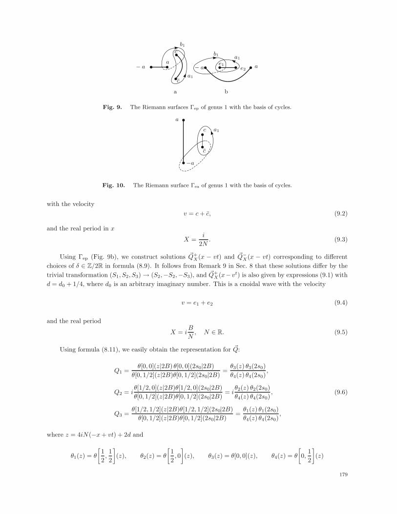
a b

Fig. 9. The Riemann surfaces Γep of genus 1 with the basis of cycles.

Fig. 10. The Riemann surface Γea of genus 1 with the basis of cycles.

with the velocityv = c + c, (9.2)

and the real period in x

X =i

2N. (9.3)

Using Γep (Fig. 9b), we construct solutions �Q+X(x − vt) and �Q−

X(x − vt) corresponding to differentchoices of δ ∈ Z/2R in formula (8.9). It follows from Remark 9 in Sec. 8 that these solutions differ by thetrivial transformation (S1, S2, S3) → (S2,−S2,−S3), and �Q+

X(x− vt) is also given by expressions (9.1) withd = d0 + 1/4, where d0 is an arbitrary imaginary number. This is a cnoidal wave with the velocity

v = e1 + e2 (9.4)

and the real period

X = iB

N, N ∈ R. (9.5)

Using formula (8.11), we easily obtain the representation for �Q:

Q1 =θ[0, 0](z|2B) θ[0, 0](2s0|2B)

θ[0, 1/2](z|2B)θ[0, 1/2](2s0|2B)=

θ3(z) θ3(2s0)θ4(z) θ4(2s0)

,

Q2 = iθ[1/2, 0](z|2B)θ[1/2, 0](2s0|2B)θ[0, 1/2](z|2B)θ[0, 1/2](2s0|2B)

= iθ2(z) θ2(2s0)θ4(z) θ4(2s0)

,

Q3 =θ[1/2, 1/2](z|2B)θ[1/2, 1/2](2s0|2B)

θ[0, 1/2](z|2B)θ[0, 1/2](2s0|2B)=

θ1(z) θ1(2s0)θ4(z) θ4(2s0)

,

(9.6)

where z = 4iN(−x + vt) + 2d and

θ1(z) = θ

[12,12

](z), θ2(z) = θ

[12, 0](z), θ3(z) = θ[0, 0](z), θ4(z) = θ

[0,

12

](z)

179

a b

Fig. 11. The Riemann surfaces Γep equivalent to the surfaces shown in Fig. 9 with the basis of cycles.

a b

Fig. 12. (a) Symmetric surfaces Γep and (b) symmetric surfaces Γea.

are Jacobi theta functions [29].We note that the solutions �QX(x − vt) = (Q1, Q2, Q3) and �Q±

X(x − vt) = (Q±1 , Q±

2 , Q±3 ) satisfy the

conditions

�QX

(x +

X

2− vt

)= (Q1,−Q2,−Q3), �Q±

X

(x +

X

2− vt

)= (−Q±

1 ,−Q±2 , Q±

3 ).

The solution �QX(x − vt) is constructed using the Riemann surface defined by the “free” boundaries of thedomains c and c, and �Q±

X(x−vt) is similarly defined by the boundaries of the domains e1 and e2. Using thecurve Γ0 with the boundaries of the domains −c and −c, we construct the solution �QX(−x− vt), and usingΓ0 with the boundaries of the domains −e1 and −e2, we construct the solution �Q±

X(−x − vt)) describingexactly the same wave moving toward the wave �QX(x − vt).

Formulas (9.2) and (9.4) demonstrate that if c = −c (if e1 = −e2), then we obtain stationary periodicsolutions with periods (9.3) and (9.5), denoted by �QX(x) (as �Q±

X(x)).Certainly, solutions of type (9.1) and (9.6) can be easily found by direct substitution of �S(x − vt) in

formula (2.1). But we note that in addition to solutions (9.1) and (9.6), we have found the corresponding Ψfunctions, which allow applying the “dressing” procedure (see Sec. 4), i.e., constructing solutions describingthe interaction of the cnoidal waves �Q with solitons, breathers, and domain walls.

The solution constructed using the curve Γ0 of genus g = 2 is a two-phase solution describing theinteraction of two cnoidal waves �QX1(x − v1t) and �QX2(x − v2t). In the general case, it is expressed interms of two-dimensional Riemann theta functions. It was shown in [30], [31] that in some cases, multiphasesolutions that are not degenerate (i.e., not reducible to the interaction of the cnoidal waves and solitons)can also be expressed in terms of elliptic functions. Several different methods for selecting solutions writtenin terms of lower-dimensional elliptic and theta functions among general finite-gap solutions were proposedin [27], [30], [32], [33]. A scheme based on reducing the multidimensional theta functions corresponding toRiemann surfaces with rich automorphism groups was given in [32].

We consider the simplest such surfaces of genera g = 2 and g = 3. The curves Γep and Γea (see Fig. 12)given by

ω2 = (λ2 − a2)(λ2 − c2)(λ2 − c2) (9.7)

180

have the involution φ : (λ, ω) → (−λ,−ω),5 i.e., the surface Γ0 is a cover of the curve Γ0/φ of genus g = 1.This is a branched two-sheet cover. The general scheme for reducing the theta function of such covers isgiven in the appendix. In the notation in the appendix, Γ = C, the surface C = C/ϕ is given by

ω21 = z(z − a2)(z − c2)(z − c2), (9.8)

and the fixed points of the involution φ are λ = ∞ on both sheets (n = 1). The cycles are A1 = a1, B1 = b1,A2 = a1′ , and B2 = b1′ . The normalized holomorphic differentials of C are

dU1 = u1 =−αλ + β

ωdλ dU2 = u1′ =

−αλ − β

ωdλ.

The normalized holomorphic differential v of the curve C given by (9.8) is

v = u1 − u1′ =2β

ωdλ =

β

ω1dz, z = λ2. (9.9)

The normalized Prym differential

w = u1 + u1′ = −2αλ

ωdλ = − α

ω2dz (9.10)

is also an elliptic differential. It is defined on the curve Cπ given by

ω22 = (z − a2)(z − c2)(z − c2). (9.11)

The curves C and Cπ (see Fig. 13) in the easy-plane case are shown together with the basis correspondingto the differentials v and w (the figures for the curve Γea are quite similar).

The constants α and β can be found from the normalization conditions

∮

A

v = 1,

∮

A

w = 1, (9.12)

where we integrate over the A cycles of the respective surfaces C given by (9.8) and Cπ given by (9.11).The period matrix of the curve C is (see formula (A.4) in the appendix)

B =12

(Π + T Π − T

Π − T Π + T

), T =

∮

B

v, Π =∮

B

w. (9.13)

It defines the theta function represented according to relation (A.8) in terms of the one-dimensional thetafunctions:

θ((z1, z2)|B) = θ[0, 0](z1 + z2|2Π) θ[0, 0](z1 − z2|2T ) +

+ θ

[12, 0](z1 + z2|2Π)θ

[12, 0](z1 − z2|2T ) =

= θ3(z1 + z2)|2Π) θ3(z1 − z2)|2T ) + θ2(z1 + z2|2Π) θ2(z1 − z2)|2T ), (9.14)

5We note that φ does not transpose the sheets of Γ0.

181

a b

Fig. 13. (a) The curve C and (b) the curve Cπ.

where θ3 and θ2 are the Jacobi theta functions. The quantities V , W , and r0 (see Theorem 6 in Sec. 7)also have a certain symmetry. It follows from identity (7.16) that

V = 4πiα

(11

), W = 8πiβ

(1

−1

). (9.15)

For the integral r0, we have

r0 =∫

s

d�U =∫

s

(u1

u1′

)=∫

φs

(φ(u1)φ(u1′)

)= −

∫

φs

(u1′

u1

)= −

∫

s

(u1′

u1

),

whence

r0 = s0

(1−1

), s0 =

∫

l

w, (9.16)

where the contour l is shown in Fig. 13a. Substituting relations (9.14)–(9.16) in (7.13), we obtain the finalexpressions for the solution �S(x, t) = �QX,τ (x, t) (see (2.15)):

A = θ3(z1|2Π) θ3(z2 − s0|2T ) + θ2(z1|2Π) θ2(z2 − s0|2Π),

B = θ3(z1|2Π) θ3(z2 + s0|2T ) + θ2(z1|2Π) θ2(z2 + s0|2Π),

C = θ3(z1|2Π) θ3(z2 − s0|2T )− θ2(z1|2Π) θ2(z2 − s0|2Π),

D = −θ3(z1|2Π) θ3(z2 + s0|2T ) + θ2(z1|2Π) θ2(z2 + s0|2Π),

(9.17)

where z1 = 4iαx + d1, z2 = 8iβt + d2, s0 is integral (9.16), and the quantities d1, d2 ∈ R are arbitrary. Inderiving this formula, we take condition (8.9) (μ = 0) and the fact that n = (1/2, 1/2) into account. Thequantities α and β are defined from formulas (9.9), (9.10), and (9.12), where v and w are the differentialsof the curves C given by (9.8) and Cπ given by (9.11), whose periods are given by (9.13).

The solution �QX,τ (x, t) given by (9.15) is a standing wave periodic in x with the period X = 1/4iα andperiodic in t with the period τ = 1/8iβ. It describes the nontrivial interaction of two waves �Q(x − vt) and�Q(−x− vt) (see (9.2)), running towards each other with equal velocities. Each of the quantities A±C andB ±D is just the product of two functions with one of them depending only on x and the other dependingonly on t. In that sense, solution (9.17) is an analogue of the known Lamb ansatz [31] for the sine-Gordonequation.

Another interesting solution in the easy-plane case corresponds to Γep (see Fig. 14). This solution canbe analyzed quite similarly to the case considered above. As a result, we obtain four (2μ = 4) standingwaves describing the interactions of various pairs of waves �Q±

X(x− vt) and �Q±X(−x− vt) (we obviously have

four combinations) given by expressions (9.17) with

z1 = 4iαx + d1 +δ1

2, z2 = 8iβt + d2 +

δ2

2,

182

Fig. 14. The symmetric surface Γep of genus 2.

where d1,2 are arbitrary numbers, Re d1,2 = 0, and δ1,2 can take the values 0 and 1.It follows from Remark 9 in Sec. 8 that only two solutions are essentially different, for instance, those

corresponding to the choices δ = (0, 0) or δ = (1, 0), i.e., solutions describing the interaction of the wavesQ+ and Q+ or Q+ and Q−. Two other standing waves differ from them trivially.

We also note that the solution describing the interaction of the stationary wave �Q(x) with the cnoidalwave �Q(x − vt) corresponds to the genus-2 surface given by the equation

ω2 = (λ2 − a2)(λ − c)(λ − c)(λ2 + d2), d ∈ R,

which does not have the additional symmetry. This interaction is therefore more complicated and is de-scribed by two-dimensional theta functions.

Finally, we consider the special solution of genus g = 3 corresponding to the surface C given by

ω2 = (λ2 − a2)(λ2 − c2)(λ2 − c2)(λ2 + d2), d ∈ R. (9.18)

As can be seen from Fig. 15 (everything is quite similar in the easy-axis case), the solution correspondingto this surface describes the interaction of the three waves �Q(x), �Q(x− vt), and �Q(−x− vt). Surface (9.18)has the involution φ : (λ, ω) → (−λ, ω), which does not transpose the infinite points ∞+ and ∞− and actson the basis of the homology group H1(C, Z) (see Fig. 15) as shown in the appendix. Here, C = C/φ, i.e.,the surface C is given by

ω21 = (z − a2)(z − c2)(z − c2)(z + d2), (9.19)

where g = 3, g = 1, n = 2, and the fixed points are 0 and ∞. The normalized differential of the surface C

isv = u1 − u1′ =

αλ

ωdλ =

α

2ω1dz, z = λ2,

and the normalized Prym differentials are given by

w1 = u1 + u1′ =β1λ

2 + γ1

ωdλ =

β1z + γ1

2ω2dz,

w2 = u2 =β2λ

2 + γ2

ωdλ =

β2z + γ2

2ω2dz,

(9.20)

where ω22 = z(z − a2)(z − c2)(z − c2)(z + d2). It hence follows with equality (7.16) taken into account that

the vectors V and W are

V = −2πi

⎛

⎜⎜⎝

β1

2β2

β1

⎞

⎟⎟⎠ , W = 4πi

⎛

⎜⎜⎝

α

0

α

⎞

⎟⎟⎠ . (9.21)

According to (A.4), for the b-period matrix, we obtain

B =

⎛

⎜⎜⎝

(Π11 + T )/2 Π12 (Π11 − T )/2

Π12 2Π22 Π12

(Π11 − T )/2 Π12 (Π11 + T )/2

⎞

⎟⎟⎠ . (9.22)

183

Fig. 15

An analysis similar to (9.16) shows that the integral

r0 =∫

s

d�U =∫

s

⎛

⎜⎜⎝

u1

u2

u1′

⎞

⎟⎟⎠ = −∫

φs

⎛

⎜⎜⎝

u1′

u2

u1

⎞

⎟⎟⎠ = −∫

s

⎛

⎜⎜⎝

u1′

u2

u1

⎞

⎟⎟⎠−∫

−2b2+a2

⎛

⎜⎜⎝

u1′

u2

u1

⎞

⎟⎟⎠

(the path s is shown in Fig. 15) is equal to

r0 =

⎛

⎜⎜⎝

s0

−1/2

s0

⎞

⎟⎟⎠+

⎛

⎜⎜⎝

Π12

−2Π22

Π12

⎞

⎟⎟⎠ , s0 =∫ 0

∞v. (9.23)

Performing the necessary calculations (see (A.8)), we finally find that for any real d1, d2, and d3, thesolution of Eq. (2.1) given by formulas (2.15) is determined by the quantities

A = θ

[(0,

12

), (0, 0)

](z1

z2

∣∣∣∣2Π)

θ[0, 0](z3 − s0|2T ) +

+ θ

[(12,12

), (0, 0)

](z1

z2

∣∣∣∣2Π)

θ

[12, 0](z3 − s0|2T ),

B = θ

[(0,

12

), (0, 0)

](z1

z2

∣∣∣∣2Π)

θ[0, 0](z3 + s0|2T ) +

+ θ

[(12,12

), (0, 0)

](z1

z2

∣∣∣∣2Π)

θ

[12, 0](z3 + s0|2T ),

C = θ

[(0,

12

),

(0,

12

)](z1

z2

∣∣∣∣2Π)

θ[0, 0](z3 − s0|2T ) +

+[(

12,12

),

(0,

12

)](z1

z2

∣∣∣∣2Π)

θ

[12, 0](z3 − s0|2T ),

D = θ

[(0,

12

),

(0,

12

)](z1

z2

∣∣∣∣2Π)

θ[0, 0](z3 + s0|2T ) +

+ θ

[(12,12

),

(0,

12

)](z1

z2

∣∣∣∣2Π)

θ

[12, 0](z3 + s0|2T ).

(9.24)

184

Fig. 16. Degeneration into the multisoliton solution: the surface Γep.

Here,z1 = −2iβ1x + d1, z2 = −2iβ2x + d2, z3 = 4iαt + d3.

This solution is periodic with the period τ = 1/4iα in t, and the dependence on x is complicated andnonperiodic.

Similarly, for any curve of genus g = 2g+n−1 having an involution with the fixed points ∞+ and ∞−,the dynamics in x is confined to the (g+n−1)-dimensional Prymian Π, and the dynamics in t is confinedto the g-dimensional Jacobian T .

10. The N -soliton solutions in the “easy plane” case

We consider the curve Γep shown in Fig. 16 together with the basis of cycles and subject the branchpoints Ej , j = 1, . . . , 2g, to the limit transition

E2k−1, E2k → λk ∈ (−a, a), k = 1, . . . , g, λ1 < λ2 < · · ·λg. (10.1)

In this case, the curve Γep degenerates into a curve of genus zero (the Riemann surface of the function√λ2 − a2), and the holomorphic differentials dUν(λ) degenerate into differentials with singularities at the

points λk:

dUν(λ) → dU0ν (λ) =

ϕ0ν(λ)√

λ2 − a2∏g

k=1(λ − λk)dλ,

where

ϕ0ν(λ) =

g∑

k=1

c0,kν λg−k.

The polynomials ϕ0ν(λ) are defined by the normalization conditions

δνμ =

∫

aμ

dU0ν (λ) = −2πi res

(dU0

ν (λ); λμ

)=

= − 2πi√λ2

μ − a2ϕ0

ν(λμ)1∏

k �=μ(λμ − λk),

and consequently

ϕ0ν(λ) = c0,1

ν

∏

k �=ν

(λ − λk), c0,1ν =

i√

λ2ν − a2

2π= −κν

2π, κν =

√a2 − λ2

ν > 0. (10.2)

Therefore, the differentials dU0ν (λ) can be written in the form

dU0ν (λ) = − 1

2π

κν√λ2 − a2(λ − λν)

dλ. (10.3)

185

By virtue of (10.3), the limit values for the coefficients c0,2ν are

c0,2ν = −c0,1

ν

∑

k �=ν

λk =12π

κν

∑

k �=ν

λk, ν = 1, . . . , g.

Hence, for the components of the vectors V and W , we have

Vν → V 0ν = −4πic0,1

ν = 2iκν ,

Wν → W 0ν = 8πi

(c0,1ν

g∑

k=1

λk + c0,2ν

)= −4iκνλν .

(10.4)

We now proceed to calculate the limit values for the b-period matrix of the basis d�U . Let ν > μ. Then

Bνμ → B0νμ = 2

∫ a

λν

dU0μ = − i

πlog

γμ − γν

γμ + γν, γν =

√a − λν

a + λν> 0. (10.5)

By the symmetry of the matrix B for ν < μ, from (10.5), we obtain

B0νμ = − i

πlog

γν − γμ

γν + γμ. (10.6)

for B0νμ. The diagonal elements of B do not have finite limits. Simple calculations show that

Re(iBνν) =1π

log |E2ν+1 − E2ν | + O(1),

i.e.,Re(iBνν) → −∞ (10.7)

for the considered limit.It remains to discuss the behavior of the vectors r and D. For the vector r, we have

rν → 12πi

r0ν + 1, r0

ν = −4πi

∫ ∞+

a

dUν(λ) = −2 logiγν + 1iγν − 1

. (10.8)

We note that Re r0ν = 0. The vector D is a free parameter, and we can prescribe its behavior at limit (10.1)

however we like. LetDν =

12Bνν +

12πi

η0ν + o(1), (10.9)

where η0ν are still arbitrary complex numbers. This completes the calculations of the limit values for all

parameters in formulas (7.13), and we can now write the limit expressions for the corresponding solutionsof the LL equation.

We represent the exponent in the definition of the series of the function θ(Ω + D + lr + kn) at l = 0, 1and k = 0, 1 in the form

πi

g∑

ν=1

Bννmν(mν + 1) + 2πi∑

ν>μ

Bνμmνmμ +

+g∑

ν=1

mν

(Vνx + Wνt + η0

ν + lr0ν + kπi + o(1)

).

186

At limit (10.1) by virtue of (10.7), only terms corresponding to the vectors m from the set of vertices {0,−1}g

of the cube [0,−1]g remain in the total infinite sum included in the definition of θ(Ω + D + lr + kn).Therefore, taking formulas (10.4)–(10.8) into account, we conclude that in limit (10.1), (10.9), we haveθ(Ω + D + lr + kn) → θl

k(x.t), where

θlk(x, t) =

∑

m∈{0,−1}g

exp{∑

ν>μ

log∣∣∣∣γν − γμ

γν + γμ

∣∣∣∣2

mνmμ

}+

+g∑

ν=1

mν(−2κνx + 4κνλνt + η0ν + lr0

ν + kπi). (10.10)

The solutions of the LL equation obtained as a result of taking the considered limit are described by theformulas

A = θ00(x, t), B = θ1

0(x, t), C = θ01(x, t), D = −θ1

1(x, t). (10.11)

The conditions for the vector η0 ensuring the realness of solution (10.11) are the last to be explored.Because all the quantities γν , κν , and λγ are real and r0

ν are purely imaginary, conjugating θlk(x, t) means

only simply replacing η0ν with η0

ν and r0ν with −r0

ν in the right-hand side of (10.10). Hence, it is easy tounderstand that relation (8.1) in the considered case is equivalent to the requirement

η0ν − η0

ν = πi + r0ν + 2πiz, z = 0,−1. (10.12)

Therefore, formulas (10.10) and (10.11) under condition (10.12) describe real solutions of the LLequation that can be parameterized by 2g real parameters (λγ , Re ην), ν = 1, . . . , g. For g = 1, we obtainthe simple soliton constructed above in Sec. 5 by the “dressing” method:

θlk = 1 + e−2κx+4κλt−η0−lr0−πik,

and consequently

S1(x, t) = − tanh(2√

a2 − λ2(x − 2λt) + Δ),

S2(x, t) = ∓λ

a

1cosh

(2√

a2 − λ2(κ − 2λt) + Δ),

S3(x, t) = ±√

a2 − λ2

a

1cosh(2κx − 4κλt + Δ)

,

(10.13)

where Δ = −Re η0 and the signs plus in S3 and minus in S2 correspond to the choice z = −1 in (10.12). Forg > 1, formulas (10.10) and (10.11) describe the processes of interactions between g simple solitons (10.13).A simple standard analysis (see, e.g., [34]) of the sum in the right-hand side of (10.10) as t → ±∞ withx − 2λjt = const shows that the jth soliton with the velocity λj and phase Δ−

j as t → −∞ has the samevelocity λj but the phase

Δ+j = Δ−

j + 2g∑

ν=j+1

log∣∣∣∣γj − γν

γj + γν

∣∣∣∣− 2j−1∑

ν=1

log∣∣∣∣γj − γν

γj + γν

∣∣∣∣

as t → +∞.

187

Fig. 17. The surface Γep in the case of ptl degeneration: complex branch points.

11. Interaction of a simple soliton with a cnoidal wave: The“easy-plane” case

We consider the “partial” degeneration of the curve Γep in the preceding section assuming g = 2:

E1 → E2 → λ0 ∈ (−a, a), E3 = E4 ≡ c, Im c �= 0. (11.1)

The “limit” curve is shown in Fig. 17. Unlike the situation in Sec. 10, the genus of the limiting curve doesnot reduce to zero. Also, one of the two holomorphic differentials remains holomorphic in this limit:

dU1(λ) → dU01 (λ) =

c0,11√

(λ2 − a2)(λ − c)(λ − c)dλ,

dU2(λ) → dU02 (λ) =

c0,12 λ + c0,2

2

(λ − λ0)√

(λ2 − a2)(λ − c)(λ − c)dλ,

(11.2)

The normalization conditions in this limit are

c0,11 =

(∫

a1

dλ√(λ2 − a2)(λ − c)(λ − c)

)−1

,

c0,12 λ0 + c0,2

2 = − 12πi

√(λ2

0 − a2)(λ0 − c)(λ0 − c),

∫

a1

c0,12 λ + c0,2

2

(λ − λ0)√

(λ20 − a2)(λ0 − c)(λ0 − c)

dλ = 0.

(11.3)

We hence obtain the representations for the components of the vectors V and W

V1 = 4πiN, V2 = −2iκ0,

W1 = −4πiNv, W2 = −4iκ0λ0,(11.4)

where

N = c0,11 =

(∫

a1

dλ√(λ2 − a2)(λ − c)(λ − c)

)−1

, v = c + c, λ0 = λ0 +v

2+ Λ0,

Λ0 = −(∫

a1

λdλ

(λ − λ0)√

(λ2 − a2)(λ − c)(λ − c)

)×

×(∫

a1

dλ

(λ − λ0)√

(λ2 − a2)(λ − c)(λ − c)

)−1

,

κ0 = −2πc0,12 = 2π

12πi

√(λ2

0 − a2)(λ0 − c)(λ0 − c)λ0 + Λ0

.

188

In the limit, the vector r and the elements B1j of the b-period matrix are also expressed in terms of ellipticintegrals:

r → r0 =∫

s

dU0(λ), B01j =

∫

b1

dU0j (λ), j = 1, 2.

Unlike the situation in Sec. 10, only the element B22 of the b-period matrix tends to i∞. Therefore, acondition of type (10.9) can be naturally imposed on the second component of the vector D, keeping thefirst component bounded:

D1 ≡ d0, D2 =1

2πiη0 +

12B22 + o(1), d0, η0 ∈ C. (11.5)

As a result, in this limit, the original sum over m ∈ Z2 in the series for θ(Ω +D+ lr + kn) is replaced with

the sum over m ∈ Z × {0,−1}, and we obtain the formula for θlk(x, t) = lim θ(Ω + D + lr + m):

θlk(x, t) = θ3

(2iN(x − vt) + d0 + lr0

1 +k

2

∣∣∣∣B011

)+

+ θ3

(2iN(x − vt) + d0 + lr0

1 +k

2− B0

12

∣∣∣∣B011

)e−2bκ0(x−2λ0t)−η0−2πilr0

2−kπi. (11.6)

We now discuss the problem of real solutions. The conjugation anti-involution τ in the consideredrealization of the curve Γep transposes the sheets and acts on the cycles aν and b1 as τaν = aν , ν = 1, 2,and τb1 = −b1 + a1. Using the same arguments as in Sec. 8, we conclude that all cj

ν are real and thequantities N , v, κ0, and λ0 are consequently also real. For the b-period matrix and the vector r, we have

B011 = −B0

11 + 1, B012 = −B0

12, rν = rν , ν = 1, 2. (11.7)

Therefore, considering C = θ01(x, t), we obtain

C = θ3(2iN(x − vt) − d 0|B011) +

+ θ3

(2iN(x − vt) − d0 − B0

12|B011

)e−2bκ0(x−2λ0t)−η0+πi.

Assuming that− d0 = d0 + r0

1 , −η0 = −η0 − 2πir02 − πi, (11.8)

we easily obtain the equality C = B. It is easy to verify that relations (10.8) also ensure that the equalityA = −D is satisfied, i.e., the corresponding solution of the LL equation is real.

We now summarize. We set

d0 = −id − 12r0i ≡ id − s, η0 = Δ − iπr0

2 − iπ

2, B0

11 = B,

where Δ and d are arbitrary real numbers and s = r01/2. A real solution of the LL equation is then given

byA = θ0

0(x, t), B = θ10(x, t), C = θ0

1(x, t), D = −θ11(x, t), (11.9)

where

θlk(x, t) = θ3

(2iN(x − vt) + id − s + 2ls +

k

2

∣∣∣∣B)

+

+ θ3

(2iN(x − vt) + id − s + 2ls +

k

2− B12

∣∣∣∣B)

e−2bκ0(x−2λ0t)−Δ+iπr02+iπ/2−2πilr0

2−kπi.

189

Fig. 18. The surface Γep in the case of partial degeneration: real branch points.

Solution (11.9) can be interpreted as describing the interaction of a simple soliton characterized by thevelocity λ0 with the cnoidal wave �QX(x− vt) with the real period X = i(2B− 1)/2N and phase velocity v.We describe this process in more detail. It follows from relations (11.9) that the presence of the soliton issignificant only in the narrow strip in the plane (x, t) around the “soliton” ray x − 2λ0t = 0, as expected.In the regions

Ω+ = {(x, t) : κ0(x − 2λ0t) � 0}, Ω− = {(x, t) : κ0(x − 2λ0t) � 0},

in particular, as x → ±∞ with fixed t (as t → ±∞ with fixed x), formulas (11.9) transform into formu-las (9.1) for the unperturbed cnoidal wave:

A = θ3(2iN(x − vt) + id − s|B),

B = θ3(2iN(x − vt) + id + s|B),

C = θ4(2iN(x − vt) + id − s|B),

D = −θ4(2iN(x − vt) + id + s|B)

(11.10)

in the region Ω− andA = θ3(2iN(x − vt) + id − s − B12|B),

B = θ3(2iN(x − vt) + id + s − B12|B),

C = −θ4(2iN(x − vt) + id − s − B12|B),

D = θ4(2iN(x − vt) + id + s − B12|B)

(11.11)

in the region Ω+ (in comparing formulas (11.10) and (11.11) with (9.1), we must take Remark 7 in Sec. 7into account).

The action on the cnoidal wave thus has two effects: the phase shift (i.e., shift of the parameter id)

B12 = B21 =∫

b2

dU01 (λ) = −2

∫ λ0

−a

N dλ√(λ2 − a2)(λ − c)(λ − c)

and the rotation (S1, S2, S3) → (−S1,−S2,−S3) through 180◦ in the plane (S1, S2). On the other hand, asformulas (11.9) and (11.4) show, the “cnoidal” background only adds 2Λ0 to the free soliton velocity 2λ0.

Remark 10. Considering the curve Γ′ep with all real branch points (see Fig. 18) instead of the curve

shown in Fig. 17, we again obtain formulas (11.6) for the complex solution of the LL equation. We need onlytake c → b, Im c = Im b = 0, everywhere. Analyzing the realness conditions only differs from the alreadyconsidered case by the fact that now τb1 = −b1 and consequently B0

11 = −B011 instead of what we have

in (11.7). The last circumstance only leads to changing the conditions for the parameter −d0 = d0+r01−1/2,

i.e.,

d0 = id − 12r01 +

14

= id − s +14,

and this in turn means that we must substitute id → id + 1/4 in formulas (11.9)-(11.11).

190

Appendix: Branched two-sheet covers and reduction ofRiemann theta functions

In this appendix, we give results concerning the reduction of the Riemann theta function containedin [35].

Let Cπ→ C be a two-sheet branched cover of genus g = 2g + n− 1 of the compact Riemann surface C

of genus g. Let Q1, . . . , Q2n ∈ C be the branch points of this cover. We let φ : C → C denote the involutionwith fixed points Q1, . . . , Q2n transposing the sheets of the cover (C = C/φ). The canonical basis of thehomology group H1(C, Z)

a1, b1 , . . . , ag, bg, ag+1, bg+1, . . . , ag+n−1, bg+n−1, a1′ , b1′ , . . . , ag′ , bg′ (A.1)

can be selected such that πa1, πb1, . . . , πag, πbg is the canonical basis of H1(C, Z):

aα′ + φaα = bα′ + φbα = 0, α = 1, . . . , g,

ai + φai = bi + φbi = 0, i = g + 1, . . . , g + n − 1.(A.2)

Here, φaα denotes the cycles obtained from aα under the action of φ. For the corresponding normalizedholomorphic differentials

u1, . . . , ug, ug+1, . . . , ug+n−1, u1′ , . . . , ug′ ,

the equalitiesuα(x) = −uα′(φ(x)), ui(x) = −ui(φ(x)), x ∈ C (A.3)

are satisfied (here α = 1, . . . , g and i = g + 1, . . . , g + n − 1).The holomorphic differentials on the surface C normalized in the basis πa1, πb1, . . . , πag, πbg are vα =

uα − uα′ , α = 1, . . . , g, and the expressions

wα = uα + uα′ , α = 1, . . . , g, wi = ui, i = g + 1, . . . , g + n − 1,

determine g+n−1 linearly independent normalized Prym differentials. We have

vα(φ(x)) = vα(x), wβ(φ(x)) = −wβ(x).

It follows from formulas (A.3) that the period matrix of C has the form

B =

⎛

⎜⎜⎝

(Παβ + Tαβ)/2 Παi (Παβ − Tαβ)/2

Πiα 2Πij Πiα

(Παβ − Tαβ)/2 Παi (Παβ + Tαβ)/2

⎞

⎟⎟⎠ , (A.4)

where α, β = 1, . . . , g,i, j = g + 1, . . . , g + n − 1, T is the period matrix of the surface C (composed ofthe differentials vα in the basis πa1, πb1, . . . , πag, πbg), and Π is the symmetric matrix of the dimension(g + n − 1) × (g + n − 1) given as

Π =

(Παβ Παj

Πiβ Πij

)=

⎛

⎜⎜⎝

∫

bβ

wα12

∫

bj

wα

∫

bβ

wi12

∫

bj

wi

⎞

⎟⎟⎠ . (A.5)

191

We consider the theta function with zero characteristics defined by matrix (A.4):

θ(z|B) =∑

m∈Zg

eπi〈Bm,m〉+2πi〈z,m〉, (A.6)

where 〈 · , · 〉 is the usual scalar product. We let S = (s1|s2|s3) denote a g-dimensional vector, where s1

and s3 are g-dimensional vectors, and s2 is a (n−1)-dimensional vector. Let t = (t1|t2) be a (g+n+1)-dimensional vector, where t1 is a g-dimensional vector and t2 is a (n−1)-dimensional vector.

We note that if the vector k ranges over the whole lattice Zg and δ = (δ|0|δ), where δ ranges over allpossible vectors consisting of the numbers 0 and 1/2, then the vector

m = N(k + δ), N =

⎛

⎜⎜⎝

I 0 I

0 I 0

I 0 −I

⎞

⎟⎟⎠ , (A.7)

also ranges over Zg (the dimensionality of the blocks in N coincides with the dimensionality of the blocksin B in (A.4)). Therefore, the sum over m in formula (A.6) can be replaced with the sum over k and δ:

〈Bm, m〉 = 〈BN(k + δ), N(k + δ)〉 = 〈NBN(k + δ), (k + δ)〉.

It is easy to see that NBN is the block matrix,

NBN =

(2Π 0

0 2T

)

(in particular, the positive definiteness of the imaginary part of Π follows from this). Consequently,

〈Bm, m〉 + 2〈z, m〉 = 〈NBN(k + δ), k + δ〉 + 2〈Nz, k + δ〉 =

= 〈2Π(k1 + (δ|0)), k1 + (δ|0)〉 + 〈2T (k2 + δ), k2 + δ〉 +

+ 2〈(z1 + z3|z2), k1 + (δ|0)〉 + 2〈z1 − z3, k2 + δ〉,

where k = (k′1|k′′

1 |k2), k1 = (k′1|k′′

1 ), and z = (z1|z2|z3). Substituting this in expressions (A.6), we obtainthe representation of the g-dimensional theta function in terms of the finite sum of the products of theg-dimensional and (g+n−1)-dimensional theta functions:

θ((z1|z2|z3)|B) =∑

δ∈ 12 Zg/2Zg

θ[(δ|0), 0]((z1 + z3|z2)|2Π) θ[δ|0](z1 − z3|2T ). (A.8)

Acknowledgments. The authors sincerely thank V. G. Bar’yakhtar, whose interest in this workessentially stimulated its writing.

REFERENCES

1. L. D. Landau and E. M. Lifschitz, “Toward a theory of the dispersion of magnetic permittivity in ferromagnetic

bodies,” in: Collected Works of L. D. Landau in Two Volumes [in Russian], Vol. 1, Nauka, Moscow (1969),

pp. 128–143.

2. L. A. Takhtajan, Phys. Lett. A, 64, 235–237 (1977).

3. A. E. Borovik, JETP Lett., 28, 581–584 (1978).

192

4. E. K. Sklyanin, “On complete integrability of the Landau–Lifshitz equation,” Preprint E-3-79, LOMI, Leningrad

(1979).

5. A. B. Shabat, Funct. Anal. Appl., 9, 244–247 (1975).

6. V. E. Zakharov and S. V. Manakov, JETP Lett., 8, 243–245 (1973).

7. I. A. Akhiezer and A. E. Borovik, JETP Lett., 52, 332–335 (1967).

8. I. A. Akhiezer, A. E. Borovik, JETP Lett., 52, 885–893 (1967).

9. A. M. Kosevich, Fiz. Met. Metalloved., 53, 420–446 (1982).

10. N. N. Bogolyubov Jr. and A. K. Prikarpatskii, “On finite-gap solutions of Heisenberg-type equations,” in: Math-

ematical Methods and Physico-Mathematical Fields (Ya. S. Podstrigach, ed.) [in Russian], Naukova Dumka,

Kiev (1983), pp. 5–11.

11. I. V. Cherednik, Math. USSR-Izv., 22, 357–377 (1984).

12. E. Date, M. Jimbo, M. Kashiwara, and T. Miwa, J. Phys. Soc. Japan, 52, 388–393 (1983).

13. M. M. Bogdan and A. S. Kovalev, JETP Lett., 31, 424–427 (1980).

14. A. V. Mikhailov, Phys. Lett. A, 92, 51–55 (1982).

15. Yu. L. Rodin, Lett. Math. Phys., 7, 3–8 (1983).

16. A. I. Bobenko, Zap. Nauchn. Sem. LOMI , 123, 58–66 (1983).

17. A. B. Borisov, Fiz. Met. Metalloved., 55, 230–234 (1983).

18. R. F. Bikbaev, A. I. Bobenko, and A. R. Its, Soviet Math. Dokl., 28, 512–516 (1983).

19. M. Jimbo, I. Miwa, and K. Ueno, Phys. D, 2, 306–352 (1981).

20. M. Jimbo and T. Miwa, Phys. D, 2, 407–448 (1981).

21. E. D. Belokolos, A. I. Bobenko, V. Z. Enol’skii, A. R. Its, and V. B. Matveev, Algebro-Geometric Approach to

Nonlinear Integrable Equations, Springer, Berlin (1994).

22. A. Gurvich and R. Kurant, Theory of Functions [in Russian], Nauka, Moscow (1968).

23. E. I. Zverovich, Russ. Math. Surveys, 26, 117–192 (1971).

24. V. B. Matveev, “Abelian functions and solitons,” Preprint H 373, Univ. Wroclaw, Wroclaw (1976).

25. B. A. Dubrovin, Russ. Math. Surveys, 36, 11–92 (1981).

26. V. E. Zaharov, S. V. Manakov, S. P. Novikov, and L. P. Pitaevskii, Theory of Solitons: The Inverse Scattering

Method [in Russian], Nauka, Moscow (1980); English transl., Plenum, New York (1984).

27. B. A. Dubrovin and S. M. Natanzon, Funct. Anal. Appl., 16, 21–33 (1982).

28. A. I. Bobenko and C. Klein, eds., Computational Approach to Riemann Surfaces (Lect. Notes Math., Vol. 2013),

Springer, Berlin (2011).

29. H. Bateman and A. Erdelyi, Higher Transcendental Functions, Vol. 3, Elliptic and Modular Functions: Lame

and Mathieu Functions, McGraw-Hill, New York (1955).

30. E. D. Belokolos and V. Z. Enol’skii, Theor. Math. Phys., 53, 1120–1127 (1982).

31. G. Forest and D.W. McLaughlin, J. Math. Phys., 23, 1248–1277 (1932).

32. E. D. Belokolos, A. I. Bobenko, V. B. Matveev, and V. Z. Enol’skii, Russ. Math. Surveys, 41, 1–49 (1986).

33. J. Zagrodzinski, J. Phys. A., 15, 3109–3118 (1982).

34. L. A. Takhtadzhyan, JETP, 66, 228–233 (1974).

35. J. D. Fay, Theta-Functions on Riemann Surfaces (Lect. Notes Math., Vol. 352), Springer, Berlin (1973).

193