Laminar Boundary Layer and Active Control of Fluid Flow
49
Department of Aerospace Sciences "Elie Carafoli" Master program Air Transport Engineering Laminar Boundary Layer and Active Control of Fluid Flow Dissertation Author: Sandra Valero Paredes Supervisor: Prof. dr. ing. Dănăilă Sterian Date: 27 th of June BUCHAREST 2018
Transcript of Laminar Boundary Layer and Active Control of Fluid Flow
Department of Aerospace Sciences "Elie Carafoli"
Master program
Air Transport Engineering
Laminar Boundary Layer and
Active Control of Fluid Flow
Dissertation
Author: Sandra Valero Paredes
Supervisor: Prof. dr. ing. Dănăilă Sterian
Date: 27th of June
BUCHAREST
2018
UNIVERSITATEA POLITEHNICA BUCURESTI
FACULTATEA DE INGINERIE AEROSPATIALA
2
CONTENTS
1 Introduction ................................................................................ 6
2 Concept of Boundary Layer ...................................................... 6
2.1 Hypothesis ............................................................................................... 7
2.2 Boundary Layer Equations ..................................................................... 8
2.2.1 Initial and boundary conditions ......................................................................................................... 9
2.3 Karman equation ................................................................................... 11
3 Plate Boundary Layer problem ............................................... 15
3.1 Plate Boundary Layer Equations .......................................................... 15
3.2 Plate Boundary Layer Conditions ......................................................... 16
3.3 Blasius Equation ................................................................................... 16
3.4 Blasius Equation Resolution with Numerical Methods ....................... 18
3.4.1 Runge-Kutta 4th order method ......................................................................................................... 19
3.4.2 Matlab Code .................................................................................................................................... 19
3.4.3 Results ............................................................................................................................................. 21
4 Control of the Boundary Layer ............................................... 23
4.1 Controlling Transition by Shaping the Airfoil ..................................... 24
4.2 Motion of the solid wall ........................................................................ 25
4.3 Controlling Transition by Suction ........................................................ 25
4.4 Controlling Separation by Suction........................................................ 26
4.5 Slit Suction ............................................................................................ 26
4.6 Tangencial blowing and suction. .......................................................... 27
4.7 Continuous suction and blowing .......................................................... 27
5 Boundary Layer Problem with Fortran Code ........................ 28
5.1 Code Description .................................................................................. 28
5.1.1 HS Panel Method ............................................................................................................................ 28
5.1.2 Printerface code ............................................................................................................................... 32
5.1.3 BLP2D code .................................................................................................................................... 32
5.2 1st Case: The Influence of the 𝒗𝒘 ......................................................... 36
UNIVERSITATEA POLITEHNICA BUCURESTI
FACULTATEA DE INGINERIE AEROSPATIALA
3
5.3 2nd Case: Study of the Optimum Section .............................................. 36
5.4 3rd Case: Value of 𝒗𝒘 ........................................................................... 36
5.5 4th Case: Influence of the Turbulence ................................................... 36
6 Numerical results ...................................................................... 37
6.1 Suction 𝒗𝒘 < 𝟎 .................................................................................... 37
6.1.1 η vs u ............................................................................................................................................... 37
6.1.2 Cf vs x .............................................................................................................................................. 38
6.1.3 δ* vs x .............................................................................................................................................. 39
6.1.4 θ vs x ............................................................................................................................................... 40
6.2 Optimum section ................................................................................... 41
6.3 Value of 𝒗𝒘 .......................................................................................... 43
6.4 Turbulent Flow and Blowing Effect ..................................................... 45
6.4.1 Cf vs x .............................................................................................................................................. 46
6.4.2 δ* vs x .............................................................................................................................................. 47
6.4.3 θ vs x ............................................................................................................................................... 48
7 Conclusions ............................................................................... 49
8 References ................................................................................. 49
UNIVERSITATEA POLITEHNICA BUCURESTI
FACULTATEA DE INGINERIE AEROSPATIALA
4
List of Figures: Figure 2-1. Development in an airfoil of the boundary layer ...............................................................................................6 Figure 2-2. Boundary layer flow along the body surface ......................................................................................................7 Figure 2-3. Calculation domain of the boundary-layer equations for external flow. ............................................................9 Figure 2-4. Boundary conditions for shear layers. (a) Boundary layer and wake of airfoil. (b) Mixing layer between
parallel streams. (c) Merging mixing layer in jet. (d) Merging boundary-layers in internal flow. ............................... 10 Figure 2-5. Boundary layer coordinates ............................................................................................................................. 11 Figure 3-1. Boundary layer on a zero-incidence flat plate .................................................................................................. 15 Figure 3-2. Code for Blasius equation (1) ........................................................................................................................... 19 Figure 3-3. Code for Blasius equation (2) ........................................................................................................................... 20 Figure 3-4. Code for Blasius equation (3) ........................................................................................................................... 20 Figure 3-5. Values of f’(η) vs values of k ............................................................................................................................ 21 Figure 3-6. Values of f’(η) vs values of η ............................................................................................................................ 22 Figure 3-7. Solution of Blasius equation (1908) ................................................................................................................. 22 Figure 4-1. Smoke flow past airfoil at zero angle of attack. ............................................................................................... 23 Figure 4-2. Same airfoil at large angle of attack with flow separation. .............................................................................. 23 Figure 4-3. High-speed photograh of boundary layer on airfoil undergoing transition. Large eddies are formed prior to
breakdown into turbulence. ..................................................................................................................................... 24 Figure 4-4. Rotating circular cylinder inside a fluid flow .................................................................................................... 25 Figure 4-5. Profile with suction slots on upper surface (indicated by arrowheads). (a) Suction off. Boundary layer is
turbulent over most of upper surface. (b) Suction on. Laminar flow restored to upper surface. ............................... 25 Figure 4-6. Multi-slotted profile of Figure 4-5 at high angle of attack. (a) Suction on. Separation is prevented. (b) No
suction. Flow totally separates from the upper surfaces. .......................................................................................... 26 Figure 4-7. Circular cylinder with a slit suction inside a fluid flow...................................................................................... 26 Figure 4-8. Tangencial blowing inside an airfoil ................................................................................................................. 27 Figure 5-1. NACA Profile Coordinates. ............................................................................................................................... 28 Figure 5-2. Panel representation of airfoil surface and notation for an airfoil incidence α ................................................ 29 Figure 6-1. Representation of η – u for station 112. .......................................................................................................... 37 Figure 6-2. Representation of Cf – x. ................................................................................................................................. 38 Figure 6-3. Comparison of the Displacement Thickness. .................................................................................................... 39 Figure 6-4. Comparison of the Momentum Thickness. ...................................................................................................... 40 Figure 6-5. Pressure Coefficient of the NACA Profile. ........................................................................................................ 41 Figure 6-6. Comparison for station 112 between two different sections for suction effect. .............................................. 42 Figure 6-7. Comparison for different values of velocity suction for station 112. ................................................................ 43 Figure 6-8. Comparison of the Ficrtion Coefficient. ........................................................................................................... 44 Figure 6-9. U+ vs Y+ for Blowing. ....................................................................................................................................... 45 Figure 6-10. Friction coeffficient versus x for turbulent flow. ............................................................................................ 46 Figure 6-11. Displacement thickness versus x for turbulent flow. ...................................................................................... 47 Figure 6-12. Theta versus x for turbulent flow. .................................................................................................................. 48

UNIVERSITATEA POLITEHNICA BUCURESTI
FACULTATEA DE INGINERIE AEROSPATIALA
5
Abstract
The present paper is a theoretical study of the main characteristics of the laminar boundary
layer in a fluid flow. It has been researched from the concept of the boundary layer to its
importance nowadays. Starting with the Navier-Stokes equations, the boundary layer problem
can be simplified through some hypothesis and it is analyzed one of the simplest cases, the
plate boundary layer problem, with numerical methods. Furthermore, it has been studied the
boundary layer problem through numerical methods with Fortran. It has been studied the types
of boundary layer control, active and passive. There cases exposed are for suction and blowing
of the boundary layer to compare and show the effects of these types of control.
UNIVERSITATEA POLITEHNICA BUCURESTI
FACULTATEA DE INGINERIE AEROSPATIALA
6
1 Introduction
The study of the boundary layer theory is one of the main studies in flud dynamics. Since its starts, all the
theory and progress has been achieved thanks to all the studies and experiments that lots of scientifics and
researchers made this past century. One of the most important developments took place in 1904, [1] when Ludwing
Plandtl showed how a theoretical treatment could be used on viscous flows in many practical cases. With some
experiments and theoretical considerations, Prandtl showed that the flow past a body can be divided into two
regions: a very thin layer close to the body (boundary layer) where the viscosity is important, and the other region
outside this layer where the effects of viscosity are not important. This concept helped to understand how important
the viscosity is in the drag problem and also it hugely reduced the mathematical difficulty. To support his theory,
Prandtl made very simple experiments in a small, self-built water channel, and he also reconnected the theory and
practice experiments. Prandtl’s frictional layer theory has proved to be extremely useful into the researching field
of fluid mechanics. Nowadays, this research still one of the most used in the fluid dynamics field, due to its
simplicity and the speed of the calculation. It is common used to solve very difficult problems because it gives a
proper estimation to the solving problem.
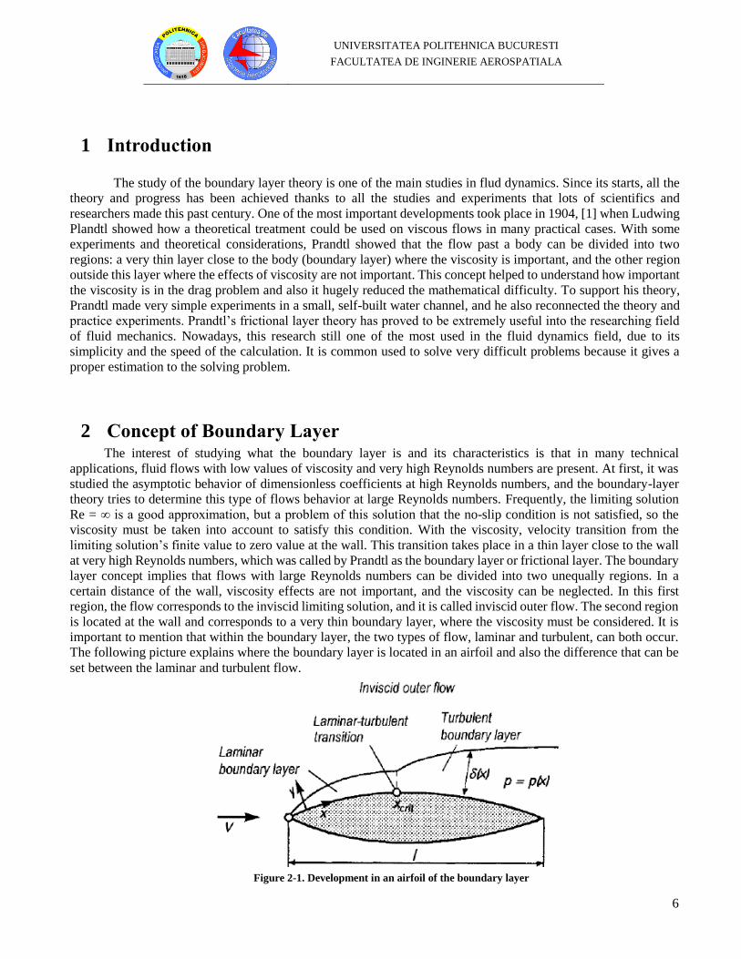
2 Concept of Boundary Layer The interest of studying what the boundary layer is and its characteristics is that in many technical
applications, fluid flows with low values of viscosity and very high Reynolds numbers are present. At first, it was
studied the asymptotic behavior of dimensionless coefficients at high Reynolds numbers, and the boundary-layer
theory tries to determine this type of flows behavior at large Reynolds numbers. Frequently, the limiting solution
Re = ∞ is a good approximation, but a problem of this solution that the no-slip condition is not satisfied, so the
viscosity must be taken into account to satisfy this condition. With the viscosity, velocity transition from the
limiting solution’s finite value to zero value at the wall. This transition takes place in a thin layer close to the wall
at very high Reynolds numbers, which was called by Prandtl as the boundary layer or frictional layer. The boundary
layer concept implies that flows with large Reynolds numbers can be divided into two unequally regions. In a
certain distance of the wall, viscosity effects are not important, and the viscosity can be neglected. In this first
region, the flow corresponds to the inviscid limiting solution, and it is called inviscid outer flow. The second region
is located at the wall and corresponds to a very thin boundary layer, where the viscosity must be considered. It is
important to mention that within the boundary layer, the two types of flow, laminar and turbulent, can both occur.
The following picture explains where the boundary layer is located in an airfoil and also the difference that can be
set between the laminar and turbulent flow.
Figure 2-1. Development in an airfoil of the boundary layer
UNIVERSITATEA POLITEHNICA BUCURESTI
FACULTATEA DE INGINERIE AEROSPATIALA
7
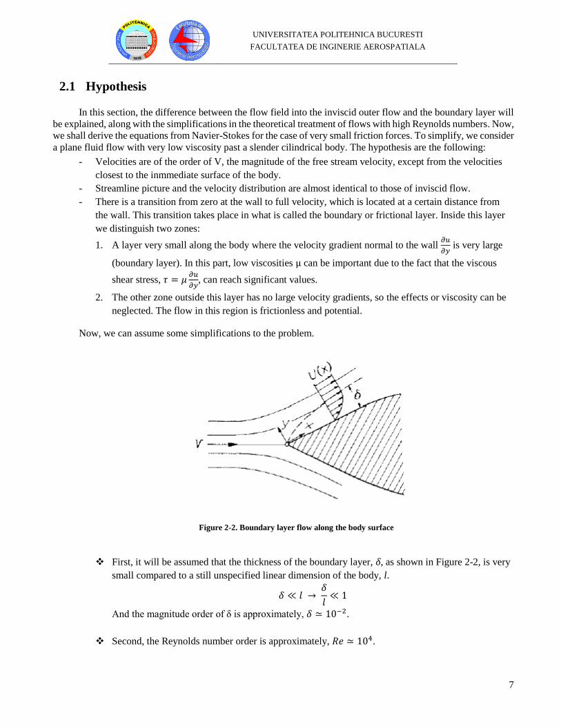
2.1 Hypothesis
In this section, the difference between the flow field into the inviscid outer flow and the boundary layer will
be explained, along with the simplifications in the theoretical treatment of flows with high Reynolds numbers. Now,
we shall derive the equations from Navier-Stokes for the case of very small friction forces. To simplify, we consider
a plane fluid flow with very low viscosity past a slender cilindrical body. The hypothesis are the following:
- Velocities are of the order of V, the magnitude of the free stream velocity, except from the velocities
closest to the inmmediate surface of the body.
- Streamline picture and the velocity distribution are almost identical to those of inviscid flow.
- There is a transition from zero at the wall to full velocity, which is located at a certain distance from
the wall. This transition takes place in what is called the boundary or frictional layer. Inside this layer
we distinguish two zones:
1. A layer very small along the body where the velocity gradient normal to the wall 𝜕𝑢
𝜕𝑦 is very large
(boundary layer). In this part, low viscosities μ can be important due to the fact that the viscous
shear stress, 𝜏 = 𝜇𝜕𝑢
𝜕𝑦, can reach significant values.
2. The other zone outside this layer has no large velocity gradients, so the effects or viscosity can be
neglected. The flow in this region is frictionless and potential.
Now, we can assume some simplifications to the problem.
Figure 2-2. Boundary layer flow along the body surface
❖ First, it will be assumed that the thickness of the boundary layer, δ, as shown in Figure 2-2, is very
small compared to a still unspecified linear dimension of the body, l.
𝛿 ≪ 𝑙 → 𝛿
𝑙≪ 1
And the magnitude order of δ is approximately, 𝛿 ≃ 10−2.
❖ Second, the Reynolds number order is approximately, 𝑅𝑒 ≃ 104.

UNIVERSITATEA POLITEHNICA BUCURESTI
FACULTATEA DE INGINERIE AEROSPATIALA
8
2.2 Boundary Layer Equations
One of the most important achievements in fluid dynamic was the deduction of the equations for the boundary
layer. These were developed with an order of magnitude analysis so that the Navier-Stokes equations of viscous
fluid flow can be simplified within the boundary layer. It is appreciated how the characteristic of the partial
differential equations becomes parabolic, instead of elliptical as they were in the original form of the full Navier-
Stokes equations. This fact greatly simplifies the problem and the equations solution. For solving the problem, the
flow is divided into an inviscid portion (outer flow) which can be solved very easily by several methods and with
that solution we can resolve the boundary layer region, which should be solved with partial differential equations.
Navier-Stokes and continuity equations for a two-dimensional steady incompressible flow in Cartesian coordinates
are the following:
𝜕𝑢
𝜕𝑥+
𝜕𝑣
𝜕𝑦= 0
𝑢𝜕𝑢
𝜕𝑥+ 𝑣
𝜕𝑢
𝜕𝑦= −
1
𝜌
𝜕𝑝
𝜕𝑥+ 𝜈 (
𝜕2𝑢
𝜕𝑥2+
𝜕2𝑢
𝜕𝑦2)
𝑢𝜕𝑣
𝜕𝑥+ 𝑣
𝜕𝑣
𝜕𝑦= −
1
𝜌
𝜕𝑝
𝜕𝑦+ 𝜈 (
𝜕2𝑣
𝜕𝑥2+
𝜕2𝑣
𝜕𝑦2)
(2.1)
(2.2)
(2.3)
In these equations, u and v are the velocity components, ρ is the fluid density, ν is the kinematic viscosity of
the fluid at a certain point and p is the pressure.
At the boundary layer, the hypothesis state that, for a large Reynolds number the flow along the surface can
be divided into the two regions, where at the boundary layer zone the viscosity effects must be considered. Velocity
components, u and v, being now as streamwise and transverse (wall normal) velocities both respectively inside the
boundary layer. With scale analysis, the final equations for the boundary layer will be reduce to the following:
𝜕𝑢
𝜕𝑥+
𝜕𝑣
𝜕𝑦= 0
𝑢𝜕𝑢
𝜕𝑥+ 𝑣
𝜕𝑢
𝜕𝑦= −
1
𝜌
𝜕𝑝
𝜕𝑥+ 𝜈
𝜕2𝑢
𝜕𝑦2
(2.4)
(2.5)
In the outer flow, the equations are given by:
𝑈𝜕𝑈
𝜕𝑥= −
1
𝜌
𝜕𝑝
𝜕𝑥
(2.6)

UNIVERSITATEA POLITEHNICA BUCURESTI
FACULTATEA DE INGINERIE AEROSPATIALA
9
2.2.1 Initial and boundary conditions
The boundary-layer equations are parabolic partial differential equations and are much easier to solve and
less costly than the Reynolds averaged Navier-Stokes equations which are elliptic. These equations are also
associated with the inviscid flow equations. The approximations used to obtain these, however, are not valid in the
same region of the flow. The boundary-layer equations apply close to the surface of a body and in wakes which
form behind the body. The inviscid flow equations apply outside the boundary-layer.
For external flow, the behavior of the boundary-layer equations is similar to the behavior of the heat
conduction equation. A small perturbation introduced in the boundary-layer diffuses instantaneously along a normal
to the wall and is transported downstream along the local streamlines in the boundary-layer. The influence domain
of a point P is limited by a line normal to the wall passing through P, by the wall and by the boundary-layer edge.
Therefore, if we wish to calculate the boundary-layer in a domain D shown in Figure 2-3, boundary or initial
conditions are required along the upstream line normal to the wall, along the and along the outer edge which defines
the domain D.
Figure 2-3. Calculation domain of the boundary-layer equations for external flow.
This choice of boundary conditions is justified by the fact that a perturbation introduced along these bounding
lines influences the flow in the calculation domain. Along the downstream boundary, no boundary condition is
required because a perturbation does not influence the calculation domain, as the velocity u is positive. If u is
negative, information can propague upstream. In addition, the two-dimensional steady boundary-layer equations
are singular at the point where the wall shear 𝜏𝑤 vanishes. This point is defined as the separation point and the
treatment of separated flow region becomes much more involved.
In external flows, the shear layer flowing in the x-direction adjoin an effectively “inviscid” freestream
extending to 𝑦 = ∞. On the lower side there may be either a solid surface, usually taken as 𝑦 = 0 as shown in
Figure 2-4a, in which case the viscous region is called a “wall shear layer”, or there may be another inviscid stream
extending to 𝑦 = −∞ (Figure 2-4b), in which case the viscous region is called a “free shear layer.”
UNIVERSITATEA POLITEHNICA BUCURESTI
FACULTATEA DE INGINERIE AEROSPATIALA
10
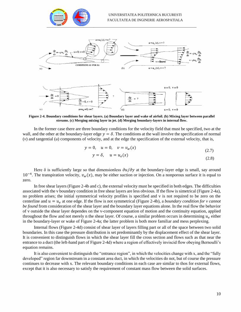
Figure 2-4. Boundary conditions for shear layers. (a) Boundary layer and wake of airfoil. (b) Mixing layer between parallel
streams. (c) Merging mixing layer in jet. (d) Merging boundary-layers in internal flow.
In the former case there are three boundary conditions for the velocity field that must be specified, two at the
wall, and the other at the boundary-layer edge 𝑦 = 𝛿. The conditions at the wall involve the specification of normal
(v) and tangential (u) components of velocity, and at the edge the specification of the external velocity, that is,
𝑦 = 0, 𝑢 = 0, 𝑣 = 𝑣𝑤(𝑥)
𝑦 = 𝛿, 𝑢 = 𝑢𝑒(𝑥)
(2.7)
(2.8)
Here δ is sufficiently large so that dimensionless 𝜕𝑢/𝜕𝑦 at the boundary-layer edge is small, say around
10−4. The transpiration velocity, 𝑣𝑤(𝑥), may be either suction or injection. On a nonporous surface it is equal to
zero.
In free shear layers (Figure 2-4b and c), the external velocity must be specified in both edges. The difficulties
associated with the v boundary condition in free shear layers are less obvious. If the flow is simetrical (Figure 2-4a),
no problem arises; the initial symmetrical velocity profiles is specified and v is not required to be zero on the
centerline and 𝑢 = 𝑢𝑒 at one edge. If the flow is not symmetrical (Figure 2-4b), a boundary condition for v cannot
be found from consideration of the shear layer and the boundary layer equations alone. In the real flow the behavior
of v outside the shear layer dependes on the v-component equation of motion and the continuity equation, applied
throughout the flow and not merely n the shear layer. Of course, a similar problem occurs in determining 𝑢𝑒 either
in the boundary-layer or wake of Figure 2-4a; the latter problem is both more familiar and mess perplexing.
Internal flows (Figure 2-4d) consist of shear layer of layers filling part or all of the space between two solid
boundaries. In this case the pressure distribution is set predominantly by the displacement effect of the shear layer.
It is convenient to distinguish flows in which the shear layer fill the cross section and flows such as that near the
entrance to a duct (the left-hand part of Figure 2-4d) where a region of effectively inviscid flow obeying Bernoulli’s
equation remains.
It is also convenient to distinguish the “entrance region”, in which the velocities change with x, and the “fully
developed” region far downstream in a constant area duct, in which the velocities do not, but of course the pressure
continues to decrease with x. The relevant boundary conditions in each case are similar to thos for external flows,
except that it is also necessary to satisfy the requirement of constant mass flow between the solid surfaces.
UNIVERSITATEA POLITEHNICA BUCURESTI
FACULTATEA DE INGINERIE AEROSPATIALA
11
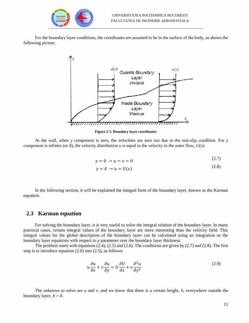
For the boundary layer conditions, the coordinates are assumed to be in the surface of the body, as shows the
following picture.
Figure 2-5. Boundary layer coordinates
At the wall, when y component is zero, the velocities are zero too due to the non-slip condition. For y
component is infinite (or δ), the velocity distribution u is equal to the velocity in the outer flow, U(x).
𝑦 = 0 → 𝑢 = 𝑣 = 0
𝑦 = 𝛿 → 𝑢 = 𝑈(𝑥)
(2.7)
(2.8)
In the following section, it will be explained the integral form of the boundary layer, known as the Karman
equation.
2.3 Karman equation
For solving the boundary layer, it is very useful to solve the integral relation of the boundary layer. In many
practical cases, certain integral values of the boundary layer are more interesting than the velocity field. This
integral values for the global description of the boundary layer can be calculated using an integration os the
boundary layer equations with respect to y parameter over the boundary layer thickness.
The problem starts with equations (2.4), (2.5) and (2.6). The conditions are given by (2.7) and (2.8). The first
step is to introduce equation (2.6) into (2.5), as follows:
𝑢𝜕𝑢
𝜕𝑥+ 𝑣
𝜕𝑢
𝜕𝑦= 𝑈
𝜕𝑈
𝜕𝑥+ 𝜈
𝜕2𝑢
𝜕𝑦2
(2.9)
The unknows to solve are u and v, and we know that there is a certain height, h, everywhere outside the
boundary layer, h > δ .
UNIVERSITATEA POLITEHNICA BUCURESTI
FACULTATEA DE INGINERIE AEROSPATIALA
12
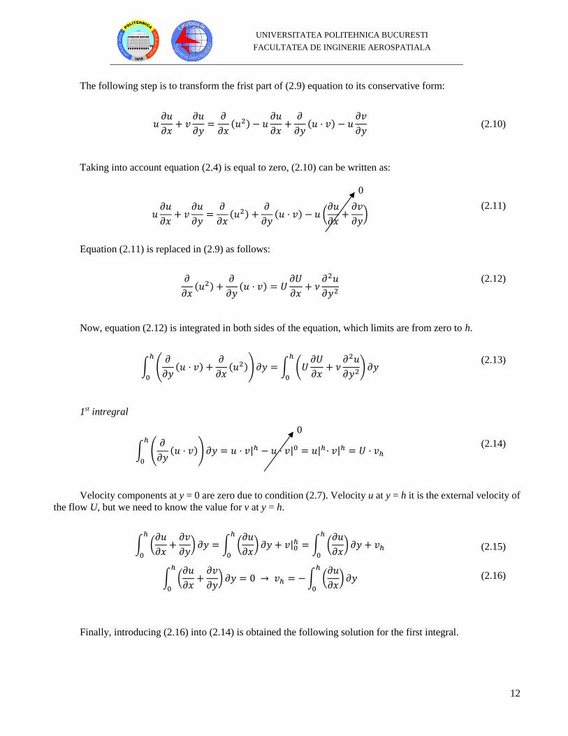
The following step is to transform the frist part of (2.9) equation to its conservative form:
𝑢𝜕𝑢
𝜕𝑥+ 𝑣
𝜕𝑢
𝜕𝑦=
𝜕
𝜕𝑥(𝑢2) − 𝑢
𝜕𝑢
𝜕𝑥+
𝜕
𝜕𝑦(𝑢 · 𝑣) − 𝑢
𝜕𝑣
𝜕𝑦
(2.10)
Taking into account equation (2.4) is equal to zero, (2.10) can be written as:
𝑢𝜕𝑢
𝜕𝑥+ 𝑣
𝜕𝑢
𝜕𝑦=
𝜕
𝜕𝑥(𝑢2) +
𝜕
𝜕𝑦(𝑢 · 𝑣) − 𝑢 (
𝜕𝑢
𝜕𝑥+
𝜕𝑣
𝜕𝑦)
(2.11)
Equation (2.11) is replaced in (2.9) as follows:
𝜕
𝜕𝑥(𝑢2) +
𝜕
𝜕𝑦(𝑢 · 𝑣) = 𝑈
𝜕𝑈
𝜕𝑥+ 𝜈
𝜕2𝑢
𝜕𝑦2
(2.12)
Now, equation (2.12) is integrated in both sides of the equation, which limits are from zero to h.
∫ (𝜕
𝜕𝑦(𝑢 · 𝑣) +
𝜕
𝜕𝑥(𝑢2))𝜕𝑦
ℎ
0
= ∫ (𝑈𝜕𝑈
𝜕𝑥+ 𝜈
𝜕2𝑢
𝜕𝑦2)𝜕𝑦ℎ
0
(2.13)
1st intregral
∫ (𝜕
𝜕𝑦(𝑢 · 𝑣)) 𝜕𝑦
ℎ
0
= 𝑢 · 𝑣|ℎ − 𝑢 · 𝑣|0 = 𝑢|ℎ· 𝑣|ℎ = 𝑈 · 𝑣ℎ
(2.14)
Velocity components at y = 0 are zero due to condition (2.7). Velocity u at y = h it is the external velocity of
the flow U, but we need to know the value for v at y = h.
∫ (𝜕𝑢
𝜕𝑥+
𝜕𝑣
𝜕𝑦) 𝜕𝑦
ℎ
0
= ∫ (𝜕𝑢
𝜕𝑥) 𝜕𝑦
ℎ
0
+ 𝑣|0ℎ = ∫ (
𝜕𝑢
𝜕𝑥)𝜕𝑦
ℎ
0
+ 𝑣ℎ
∫ (𝜕𝑢
𝜕𝑥+
𝜕𝑣
𝜕𝑦) 𝜕𝑦
ℎ
0
= 0 → 𝑣ℎ = −∫ (𝜕𝑢
𝜕𝑥)𝜕𝑦
ℎ
0
(2.15)
(2.16)
Finally, introducing (2.16) into (2.14) is obtained the following solution for the first integral.
0
0

UNIVERSITATEA POLITEHNICA BUCURESTI
FACULTATEA DE INGINERIE AEROSPATIALA
13
∫ (𝜕
𝜕𝑦(𝑢 · 𝑣)) 𝜕𝑦
ℎ
0
= 𝑈 · 𝑣ℎ = −𝑈∫ (𝜕𝑢
𝜕𝑥) 𝜕𝑦
ℎ
0
(2.17)
2nd integral
∫ (𝜈𝜕2𝑢
𝜕𝑦2)𝜕𝑦ℎ
0
= ∫𝜕
𝜕𝑦(𝜈
𝜕𝑢
𝜕𝑦)𝜕𝑦
ℎ
0
(2.18)
For this integral, the shear stress definition is needed.
𝜏 = 𝜇𝜕𝑢
𝜕𝑦= 𝜌
𝜇
𝜌
𝜕𝑢
𝜕𝑦= 𝜌 · 𝜈
𝜕𝑢
𝜕𝑦 →
𝜏
𝜌= 𝜈
𝜕𝑢
𝜕𝑦
∫𝜕
𝜕𝑦(𝜈
𝜕𝑢
𝜕𝑦)𝜕𝑦
ℎ
0
= ∫𝜕
𝜕𝑦(𝜏
𝜌) 𝜕𝑦
ℎ
0
=𝜏ℎ − 𝜏𝑤
𝜌= −
𝜏𝑤
𝜌
(2.19)
(2.20)
The shear stress at a certain height, h, is zero because there is no variation with y axis in the velocity
distribution, u. At the end, the value of this integral will be minus the wall shear stress divided by the density.
3rd integral
The integrals that have been already solved are replaced in the main equation (2.13).
∫ (𝜕
𝜕𝑥(𝑢2)) 𝜕𝑦
ℎ
0
− 𝑈∫ (𝜕𝑢
𝜕𝑥)𝜕𝑦
ℎ
0
= ∫ (𝑈𝜕𝑈
𝜕𝑥) 𝜕𝑦
ℎ
0
−𝜏𝑤
𝜌
∫ (𝜕
𝜕𝑥(𝑢2) − 𝑈 (
𝜕𝑢
𝜕𝑥) − 𝑈 (
𝜕𝑈
𝜕𝑥))𝜕𝑦
ℎ
0
= −𝜏𝑤
𝜌
∫ (𝜕
𝜕𝑥(𝑢2) −
𝜕
𝜕𝑥(𝑈 · 𝑢) + 𝑢 (
𝜕𝑈
𝜕𝑥) − 𝑈 (
𝜕𝑈
𝜕𝑥))𝜕𝑦
ℎ
0
= −𝜏𝑤
𝜌
(2.21)
(2.22)
(2.23)
Now, we need two definitions to express equation (2.23) to its final form.
0
UNIVERSITATEA POLITEHNICA BUCURESTI
FACULTATEA DE INGINERIE AEROSPATIALA
14
- Displacement thickness, 𝛿1
𝛿1 = 𝛿∗ =1
𝑈∫ (𝑈 − 𝑢)𝜕𝑦
𝛿(∞)
0
(2.24)
- Momentum thickness, 𝛿2
𝛿2 = 𝜃 =1
𝑈2∫ 𝑢 (𝑈 − 𝑢)𝜕𝑦
𝛿(∞)
0
(2.25)
Finally, replacing these two definitions into equation (2.23), the momentum-integral equation for plane,
incompressible boundary layers is shown.
∫ (𝜕
𝜕𝑥(𝑢2 − (𝑈 · 𝑢)) +
𝜕𝑈
𝜕𝑥(𝑢 − 𝑈)) 𝜕𝑦
ℎ
0
= −𝜏𝑤
𝜌
∫ (𝜕
𝜕𝑥(𝑢(𝑢 − 𝑈) +
𝜕𝑈
𝜕𝑥(𝑢 − 𝑈)) 𝜕𝑦
ℎ
0
= −𝜏𝑤
𝜌
𝜕
𝜕𝑥∫ ((𝑢(𝑢 − 𝑈))𝑑𝑦 +
𝜕𝑈
𝜕𝑥∫ (𝑢 − 𝑈)
ℎ
0
𝜕𝑦ℎ
0
= −𝜏𝑤
𝜌
−𝜕
𝜕𝑥(𝑈2 · 𝜃) − 𝑈 ·
𝜕𝑈
𝜕𝑥· 𝛿∗ = −
𝜏𝑤
𝜌
𝜕
𝜕𝑥(𝑈2 · 𝜃) + 𝛿∗ · 𝑈
𝜕𝑈
𝜕𝑥=
𝜏𝑤
𝜌
(2.26)
(2.27)
(2.28)
(2.29)
(2.30)
The momentum-integral equation is very useful to obtain two different type of results. This equation in this
form is valid for both laminar and turbulent boundary layers.
1. If 𝑢(𝑥, 𝑦) is known, the wall shear stress can be calculated with equation (2.30) with more precision
and less error than using the definition of the derivative (2.19).
Friction coefficient and drag friction can be also obtained.
𝐶𝑓 =𝜏𝑤
𝜌
2𝑈2
𝐷𝑓 = ∫ 𝜏𝑤 𝜕𝑠𝑙
0
(2.31)
(2.32)
UNIVERSITATEA POLITEHNICA BUCURESTI
FACULTATEA DE INGINERIE AEROSPATIALA
15
Being l the total length of the body surface.
2. Displacement thickness, momentum thickness and boundary layer thickness can be computed using
the momentum-integral equation. These parameters are also related with drag friction and they
provide very useful information about the boundary layer. This can be study more accurate with the
Karman-Polhausen method.
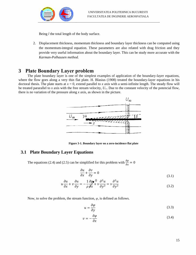
3 Plate Boundary Layer problem The plate boundary layer is one of the simplest examples of application of the boundary-layer equations,
where the flow goes along a very thin flat plate. H. Blasius (1908) treated the boundary-layer equations in his
doctoral thesis. The plate starts at x = 0, extend parallel to x axis with a semi-infinite length. The steady flow will
be treated pararallel to x axis with the free stream velocity, U∞. Due to the constant velocity of the potencial flow,
there is no variation of the pressure along x axis, as shown in the picture.
Figure 3-1. Boundary layer on a zero-incidence flat plate
3.1 Plate Boundary Layer Equations
The equations (2.4) and (2.5) can be simplified for this problem with 𝜕𝑝
𝜕𝑥= 0
𝜕𝑢
𝜕𝑥+
𝜕𝑣
𝜕𝑦= 0
𝑢𝜕𝑢
𝜕𝑥+ 𝑣
𝜕𝑢
𝜕𝑦= −
1
𝜌
𝜕𝑝
𝜕𝑥+ 𝜈
𝜕2𝑢
𝜕𝑦2= 𝜈
𝜕2𝑢
𝜕𝑦2
(3.1)
(3.2)
Now, to solve the problem, the stream function, φ, is defined as follows.
𝑢 =𝜕𝜑
𝜕𝑦
𝑣 = −𝜕𝜑
𝜕𝑥
(3.3)
(3.4)
0
UNIVERSITATEA POLITEHNICA BUCURESTI
FACULTATEA DE INGINERIE AEROSPATIALA
16
3.2 Plate Boundary Layer Conditions
The conditions that we impose to solve the problem are the following:
𝑦 = 0 → 𝑢 = 𝑣 = 0
𝑦 = 𝛿 → 𝑢 = 𝑈∞
(3.5)
(3.6)
The system shown in Figure 3-1 has no characteristic length, so we assume that the velocity distributions at
different distances from the leading edge are similar to one another. For u velocity profile, we use U∞ as the scaling
factor, while for y we use the “boundary layer thickness” δ(x), which increases with x distance. Actually, δ(x) is
not the boundary-layer thickness but a scaled mesure of it which is equal to the boundary-layer thickness up to
some numerical factor. We use one similarity law for the velocity profile, where 𝜑(𝜂) is independent of x:
𝑢
𝑈∞= 𝜑(𝜂)
𝜂 =𝑦
𝛿(𝑥)
(3.7)
(3.8)
The resolution of the two partial equations (3.1) and (3.2) are transformed by similarity transformation to
lead to an ordinary differential equation for the stream function, called Blasius equation, where all the steps will be
explained in the following section.
3.3 Blasius Equation
The first step for the plate boundary-layer resolution is to change equations (3.1) and (3.2) with the stream
function definitions (3.3) and (3.4).
𝜕
𝜕𝑥(𝜕𝜑
𝜕𝑦) +
𝜕
𝜕𝑦(−
𝜕𝜑
𝜕𝑥) = 0
(𝜕𝜑
𝜕𝑦) ·
𝜕
𝜕𝑥(𝜕𝜑
𝜕𝑦) + (−
𝜕𝜑
𝜕𝑥)
𝜕
𝜕𝑦(𝜕𝜑
𝜕𝑦) = 𝜈
𝜕2
𝜕𝑦2(𝜕𝜑
𝜕𝑦)
(3.9)
(3.10)
The conditions change to the following expressions:
𝑦 = 0 →𝜕𝜑
𝜕𝑦= −
𝜕𝜑
𝜕𝑥= 0
𝑦 = 𝛿 →𝜕𝜑
𝜕𝑦= 𝑈∞
(3.11)
(3.12)
The similarity variable is defined as follows:
𝜂 = 𝑦 √𝑈∞
𝜈 𝑥
(3.13)

UNIVERSITATEA POLITEHNICA BUCURESTI
FACULTATEA DE INGINERIE AEROSPATIALA
17
The continuity equation can be integrated introducing a stream function, 𝜓(𝑥, 𝑦).
𝜓(𝑥, 𝑦) = √𝑈∞ · 𝜈 · 𝑥 · 𝑓(𝜂)
(3.14)
where 𝑓(𝜂) is the dimensionless stream function.
The next step is to transform the velocity components using the stream function and the similarity variable.
𝑢 =𝜕𝜑
𝜕𝑦=
𝜕𝜑
𝜕𝜂·𝜕𝜂
𝜕𝑦
𝑣 = −𝜕𝜑
𝜕𝑥= −(
𝜕𝜑
𝜕𝑥+
𝜕𝜑
𝜕𝜂·𝜕𝜂
𝜕𝑥)
(3.15)
(3.16)
Now, we need to derive the stream function and the similarity variable to obtain the final equation.
𝜕𝜑
𝜕𝜂= √𝑈∞ · 𝜈 · 𝑥 · 𝑓′(𝜂)
𝜕𝜂
𝜕𝑦= √
𝑈∞
𝜈 𝑥
(3.17)
(3.18)
For v velocity distribution we have the following expressions.
−𝜕𝜑
𝜕𝑥= −
𝜕
𝜕𝑥(√𝑈∞ · 𝜈 · 𝑥 · 𝑓(𝜂)) = −(
𝜕
𝜕𝑥(√𝑈∞ · 𝜈 · 𝑥 ) · 𝑓(𝜂) + √𝑈∞ · 𝜈 · 𝑥 ·
𝜕
𝜕𝑥𝑓(𝜂))
𝜕𝜂
𝜕𝑥= −
𝜂
2·1
𝑥
−𝜕𝜑
𝜕𝑥= −√𝑈∞ · 𝜈 ((
1
2 √𝑥) · 𝑓(𝜂) + √𝑥 · 𝑓′(𝜂) · (−
𝜂
2·1
𝑥))
(3.19)
(3.20)
(3.21)
All the derivates for the stream function needed for replacing them into equation (3.10) are the following:
𝜕𝜑
𝜕𝑦= 𝑈∞ · 𝑓′(𝜂)
𝜕2𝜑
𝜕𝑦2= 𝑈∞ · 𝑓′′(𝜂) · √
𝑈∞
𝜈 𝑥
𝜕3𝜑
𝜕𝑦3=
𝑈∞2
𝜈 · 𝑥· 𝑓′′′(𝜂)
𝜕𝜑
𝜕𝑥= √𝑈∞ · 𝜈 ((
1
2 √𝑥) · 𝑓(𝜂) + √𝑥 · 𝑓′(𝜂) · (−
𝜂
2·1
𝑥))
(3.22)
(3.23)
(3.24)
(3.25)
UNIVERSITATEA POLITEHNICA BUCURESTI
FACULTATEA DE INGINERIE AEROSPATIALA
18
𝜕
𝜕𝑥(𝜕𝜑
𝜕𝑦) =
𝜕
𝜕𝑥(𝑈∞ · 𝑓′(𝜂)) = 𝑈∞ · 𝑓′′(𝜂) · (−
𝜂
2·1
𝑥)
(3.26)
Setting all the equation together in equation (3.10) we obtain the Blasius equation.
𝑓′′′(𝜂) +1
2𝑓′′(𝜂) · 𝑓(𝜂) = 0 (3.27)
3.4 Blasius Equation Resolution with Numerical Methods
Blasius equation is an ordinary differential equation, nonlinear and third order. The three boundary
conditions (3.11) and (3.12) are sufficient to determine the solution. This solution can be done by using numerical
methods, as Runge-Kutta 4th order method.
Instead of solving the boundary value problem, the initial values at η = 0,
𝑓(0) = 𝑓′(0) = 0 (3.28)
and estimated value,
𝑓′′(0) = 𝑘 (3.29)
are solved until the following boundary condition is true,
𝑓′(∞) = 1 (3.30)
The problem is solved with Matlab®, defining the initial system as follows:
𝑓(𝜂) = 𝑔1
𝑓′(𝜂) = 𝑔2
𝑓′′(𝜂) = 𝑔3
(3.31)
(3.32)
(3.33)
Also the derivates are:
𝑔1′ = 𝑔2
𝑔2′ = 𝑔3
𝑔3′ = −
1
2𝑔1𝑔3
(3.31)
(3.32)
(3.33)
This last one, (3.33) is obtained using the Blasius equation:
𝑔3′ +
1
2𝑔1 · 𝑔3 = 0 → 𝑔3
′ = −1
2𝑔1 · 𝑔3 (3.34)
UNIVERSITATEA POLITEHNICA BUCURESTI
FACULTATEA DE INGINERIE AEROSPATIALA
19
3.4.1 Runge-Kutta 4th order method
Runge-Kutta method, is an iterative numerical method for solving diferential equations which solves
approaching to the solution of an initial value problem. Its expressions for the fourth order method are the following:
𝑦′ = 𝑔′ = 𝑓(𝑥, 𝑦) = 𝐵 · 𝑔𝑇 = (
0 1 00 0 1
−𝑔3
20 0
) · [𝑔1 𝑔2 𝑔3]𝑇 = [𝑔2 𝑔3
−𝑔3𝑔1
2]𝑇
𝑦(𝑥0) = 𝑦0 → 𝑔0𝑇 = [0 0 𝑘]𝑇
𝑦𝑖+1 = 𝑦𝑖 +1
6ℎ(𝑘1 + 2𝑘2 + 2𝑘3 + 𝑘4)
(3.35)
(3.36)
(3.37)
The values of the parameters are calculated:
𝑘1 = 𝑓(𝑥𝑖, 𝑦𝑖) = 𝐵𝑖 · 𝑔𝑖𝑇
𝑘2 = 𝑓 (𝑥𝑖 +1
2ℎ, 𝑦𝑖 +
1
2𝑘1ℎ) = 𝐵𝑖 · (𝑔𝑖 +
1
2𝑘1ℎ)
𝑘3 = 𝑓 (𝑥𝑖 +1
2ℎ, 𝑦𝑖 +
1
2𝑘2ℎ) = 𝐵𝑖 · (𝑔𝑖 +
1
2𝑘2ℎ)
𝑘4 = 𝑓(𝑥𝑖 + ℎ, 𝑦𝑖 + 𝑘3ℎ) = 𝐵𝑖 · (𝑔𝑖 + 𝑘3ℎ)
(3.38)
(3.39)
(3.40)
(3.41)
In this way, the next value 𝑦𝑖+1 is obtained by the present value 𝑦𝑖 plus the product of the interval size, h,
multiplied for an estimated gradient. This method of 4th order means that the step error is of the order of O(h5) while
the total error that it has is O(h4). So that, the convergence of the method is O(h4) order, that is the reason why it is
used in computational methods.
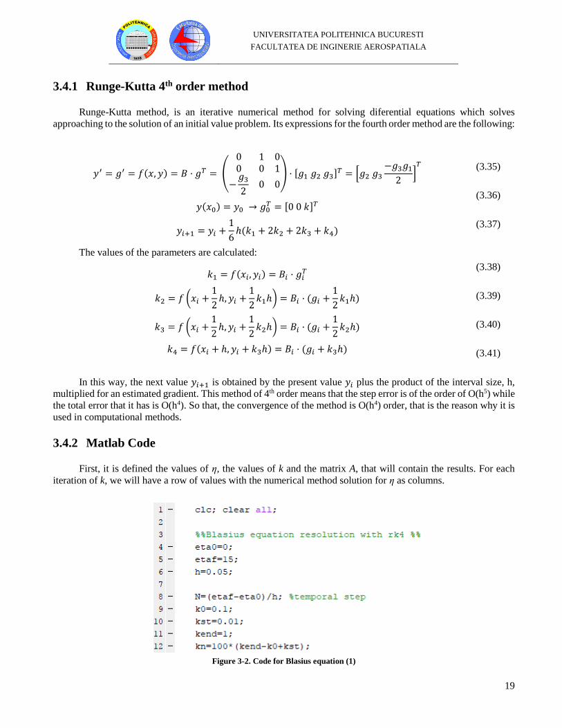
3.4.2 Matlab Code
First, it is defined the values of η, the values of k and the matrix A, that will contain the results. For each
iteration of k, we will have a row of values with the numerical method solution for η as columns.
Figure 3-2. Code for Blasius equation (1)
UNIVERSITATEA POLITEHNICA BUCURESTI
FACULTATEA DE INGINERIE AEROSPATIALA
20
The main loop is for each k, with the initial conditions of equation (3.36). The second loop is the Runge-
Kutta of 4th order method, where the variables has been explained in the equations from (3.35) to (3.41). The results
for 𝑓′(𝜂) = 𝑔2 are saved in A matrix.
Figure 3-3. Code for Blasius equation (2)
This part of the code shows how the final results from the loop are safed into a vector f15 and are plotted
with a line where 𝑓′(𝜂) = 1 to obtain the value of k for this result.
Figure 3-4. Code for Blasius equation (3)
UNIVERSITATEA POLITEHNICA BUCURESTI
FACULTATEA DE INGINERIE AEROSPATIALA
21
3.4.3 Results
The results obtained are the two plots that are shown.
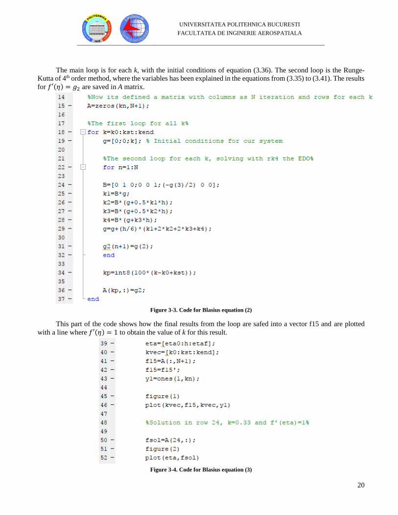
Figure 3-5. Values of f’(η) vs values of k
In the Figure 3-5, the solution to the problem is shown. For the boundary condition 𝑓′(∞) = 1, the value of
the initial value problem is 𝑘 = 0.33. So that, the next figure will show the distribution of 𝑓′(𝜂) vs 𝜂.
0.1 0.2 0.3 0.4 0.5 0.6 0.7 0.8 0.9 10.4
0.6
0.8
1
1.2
1.4
1.6
1.8
2
2.2
2.4
k
f’(η
)
UNIVERSITATEA POLITEHNICA BUCURESTI
FACULTATEA DE INGINERIE AEROSPATIALA
22
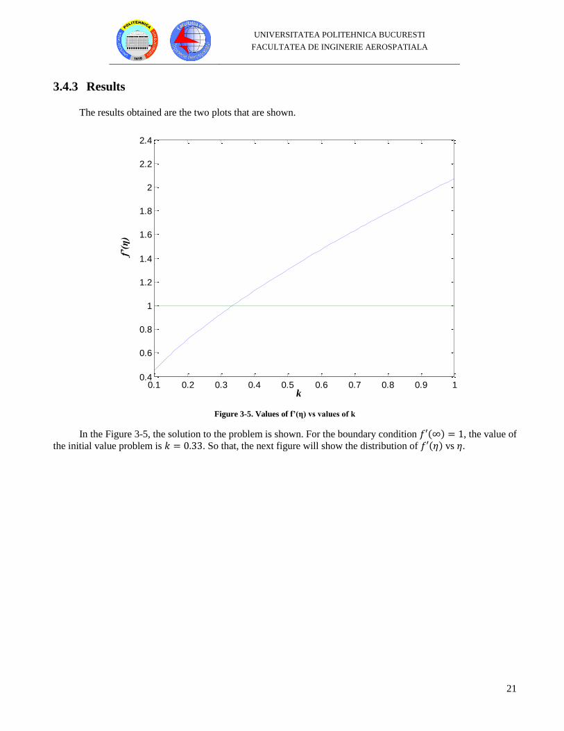
Figure 3-6. Values of f’(η) vs values of η
Finally, the value of 𝜂 = 5 is the one that accomplish the boundary condition imposed (3.30). This solution
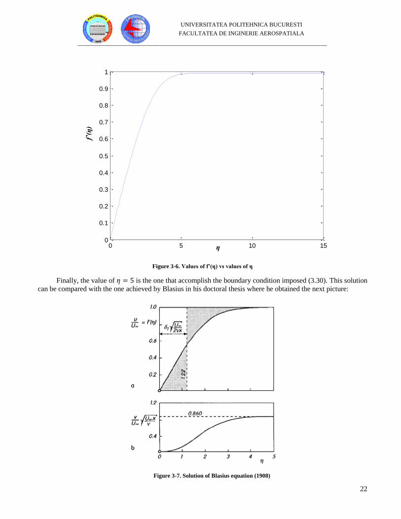
can be compared with the one achieved by Blasius in his doctoral thesis where he obtained the next picture:
Figure 3-7. Solution of Blasius equation (1908)
0 5 10 150
0.1
0.2
0.3
0.4
0.5
0.6
0.7
0.8
0.9
1
f’(η
)
η
UNIVERSITATEA POLITEHNICA BUCURESTI
FACULTATEA DE INGINERIE AEROSPATIALA
23
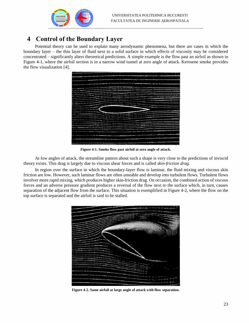
4 Control of the Boundary Layer Potential theory can be used to explain many aerodynamic phenomena, but there are cases in which the
boundary layer – the thin layer of fluid next to a solid surface in which effects of viscosity may be considered
concentrated – significantly alters theoretical predictions. A simple example is the flow past an airfoil as shown in
Figure 4-1, where the airfoil section is in a narrow wind tunnel at zero angle of attack. Kerosene smoke provides
the flow visualization [4].
Figure 4-1. Smoke flow past airfoil at zero angle of attack.
At low angles of attack, the streamline pattern about such a shape is very close to the predictions of inviscid
theory exists. This drag is largely due to viscous shear forces and is called skin-friction drag.
In region over the surface in which the boundary-layer flow is laminar, the fluid mixing and viscous skin
friction are low. However, such laminar flows are often unstable and develop into turbulent flows. Turbulent flows
involver more rapid mixing, which produces higher skin-friction drag. On occasion, the combined action of viscous
forces and an adverse pressure gradient produces a reversal of the flow next to the surface which, in turn, causes
separation of the adjacent flow from the surface. This situation is exemplified in Figure 4-2, where the flow on the
top surface is separated and the airfoil is said to be stalled.
Figure 4-2. Same airfoil at large angle of attack with flow separation.
UNIVERSITATEA POLITEHNICA BUCURESTI
FACULTATEA DE INGINERIE AEROSPATIALA
24
The presence of the boundary layer has produced many design problems in all areas of fluid mechanics.
However, the most intensive investigations have been directed towards its effect upon the lift and drag of wings.
The techniques that have been developed to manipulate the boundary layer, either to increase the lift or decrease
drag, are classified under the general heading of boundary-layer control.
Two boundary-layer phenomena for which controls have been sought are the transition of a laminar layer to
a turbulent flow and the separation of the entire flow from the surface. By maintaining as much of the boundary
layer in laminar state as possible, one can reduce the skin friction. By preventing separation, it is possible to increase
the lifting effectiveness and reduce the pressure drag. Sometimes the same control can serve both functions.
To sum up, flow control referes to the ability to alter flows with the aim of achieving a desired effect,
examples of flow control applications include drag reduction, noise attenuation, improved mixing, or increased
combustion efficiency, among many other industrial applications.
A laminar boundary-layer forms when a real (viscous) fluid flow past a solid body. The boundary layer
separation represens a major proble which constrains the design of aircraft device. It is characterized by a loss of
kinetic energy near solid surface and it depends on the flow regime, which is either laminar or turbulent. Moreover,
it is necessary to have a flow separation control. The ways for separation control can be splitted into:
- Passive Control: Vortex generators, Flaps/Slats, Absorbant Surface, Ribles.
- Active Control: Mobile surface, Planform control, Jets, Advanced controls.
Next sections will explain different types of boundary-layer control. The main focuss of this research is
active control of the boundary-layer with suction and blowing.
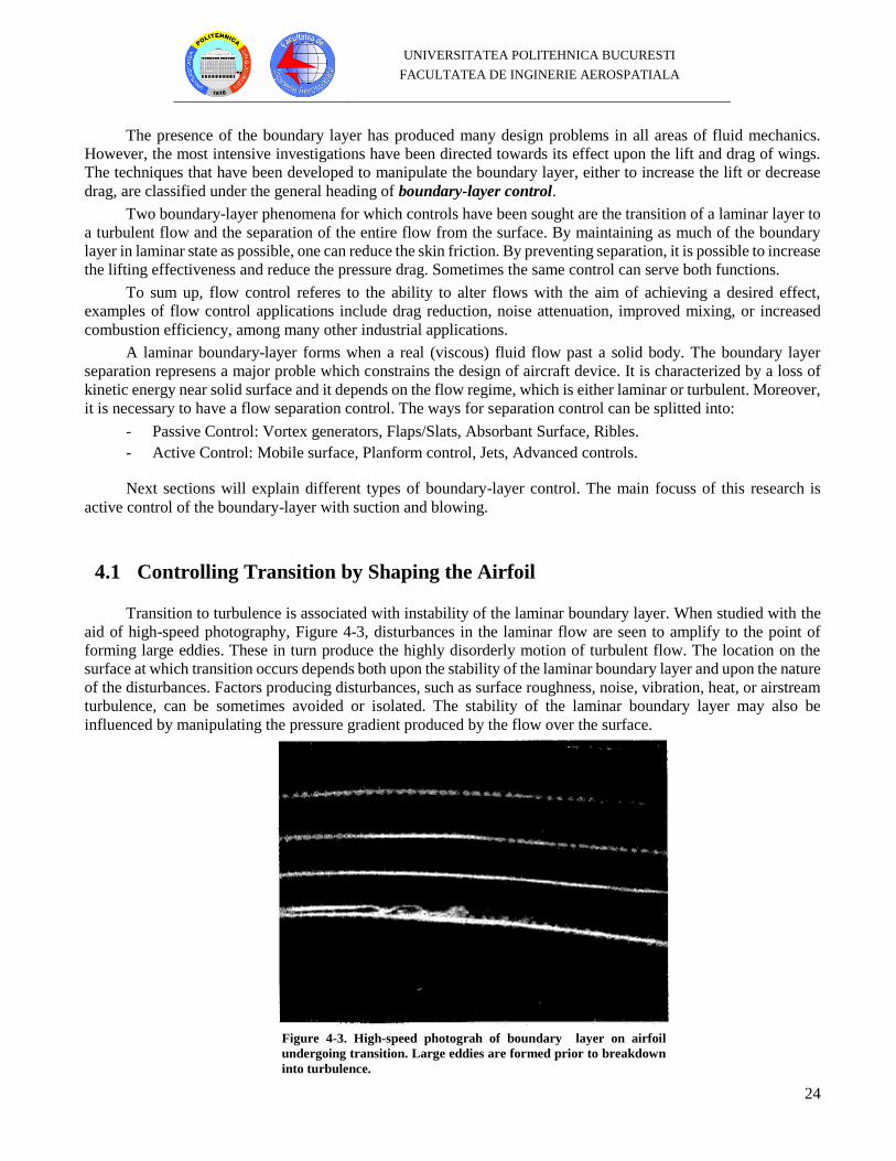
4.1 Controlling Transition by Shaping the Airfoil
Transition to turbulence is associated with instability of the laminar boundary layer. When studied with the
aid of high-speed photography, Figure 4-3, disturbances in the laminar flow are seen to amplify to the point of
forming large eddies. These in turn produce the highly disorderly motion of turbulent flow. The location on the
surface at which transition occurs depends both upon the stability of the laminar boundary layer and upon the nature
of the disturbances. Factors producing disturbances, such as surface roughness, noise, vibration, heat, or airstream
turbulence, can be sometimes avoided or isolated. The stability of the laminar boundary layer may also be
influenced by manipulating the pressure gradient produced by the flow over the surface.
Figure 4-3. High-speed photograh of boundary layer on airfoil
undergoing transition. Large eddies are formed prior to breakdown
into turbulence.
UNIVERSITATEA POLITEHNICA BUCURESTI
FACULTATEA DE INGINERIE AEROSPATIALA
25
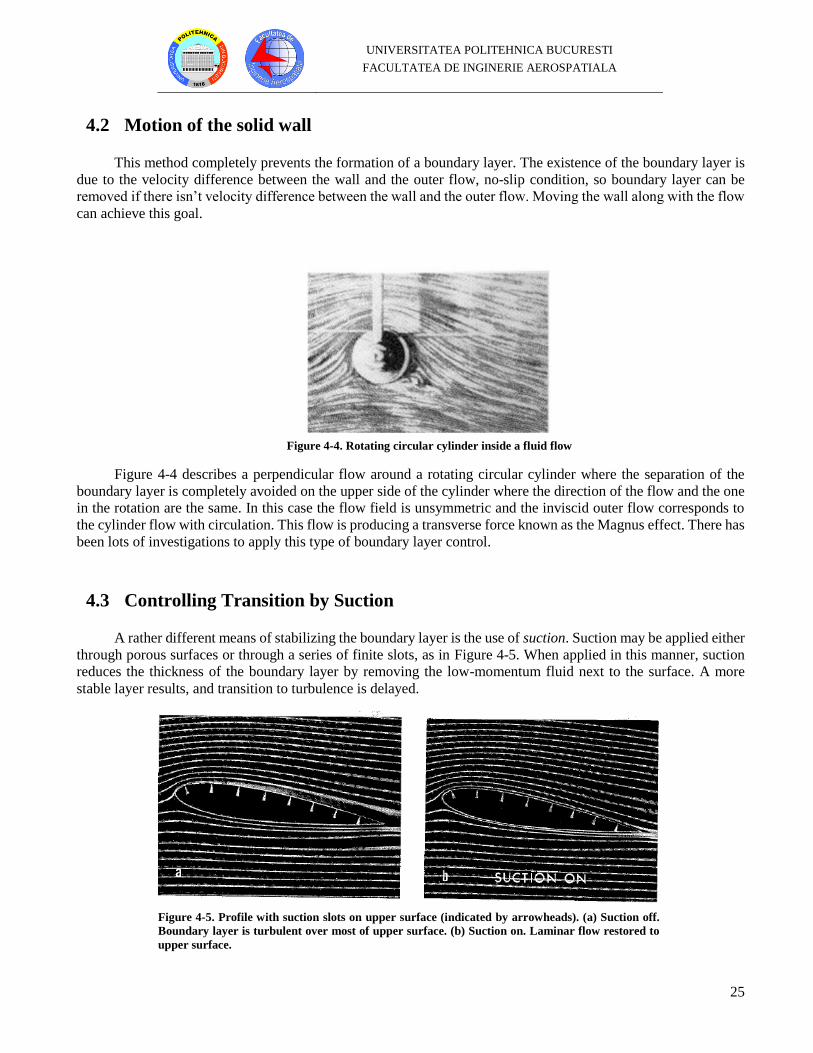
4.2 Motion of the solid wall
This method completely prevents the formation of a boundary layer. The existence of the boundary layer is
due to the velocity difference between the wall and the outer flow, no-slip condition, so boundary layer can be
removed if there isn’t velocity difference between the wall and the outer flow. Moving the wall along with the flow
can achieve this goal.
Figure 4-4. Rotating circular cylinder inside a fluid flow
Figure 4-4 describes a perpendicular flow around a rotating circular cylinder where the separation of the
boundary layer is completely avoided on the upper side of the cylinder where the direction of the flow and the one
in the rotation are the same. In this case the flow field is unsymmetric and the inviscid outer flow corresponds to
the cylinder flow with circulation. This flow is producing a transverse force known as the Magnus effect. There has
been lots of investigations to apply this type of boundary layer control.
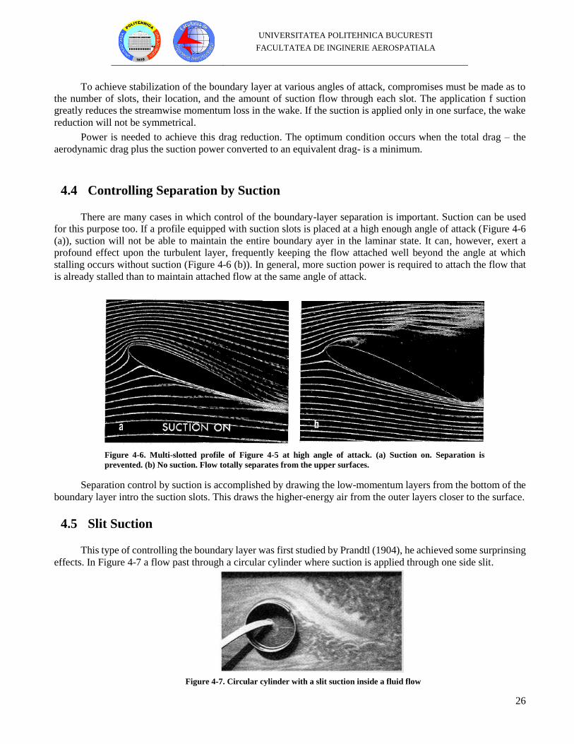
4.3 Controlling Transition by Suction
A rather different means of stabilizing the boundary layer is the use of suction. Suction may be applied either
through porous surfaces or through a series of finite slots, as in Figure 4-5. When applied in this manner, suction
reduces the thickness of the boundary layer by removing the low-momentum fluid next to the surface. A more
stable layer results, and transition to turbulence is delayed.
Figure 4-5. Profile with suction slots on upper surface (indicated by arrowheads). (a) Suction off.
Boundary layer is turbulent over most of upper surface. (b) Suction on. Laminar flow restored to
upper surface.
UNIVERSITATEA POLITEHNICA BUCURESTI
FACULTATEA DE INGINERIE AEROSPATIALA
26
To achieve stabilization of the boundary layer at various angles of attack, compromises must be made as to
the number of slots, their location, and the amount of suction flow through each slot. The application f suction
greatly reduces the streamwise momentum loss in the wake. If the suction is applied only in one surface, the wake
reduction will not be symmetrical.
Power is needed to achieve this drag reduction. The optimum condition occurs when the total drag – the
aerodynamic drag plus the suction power converted to an equivalent drag- is a minimum.
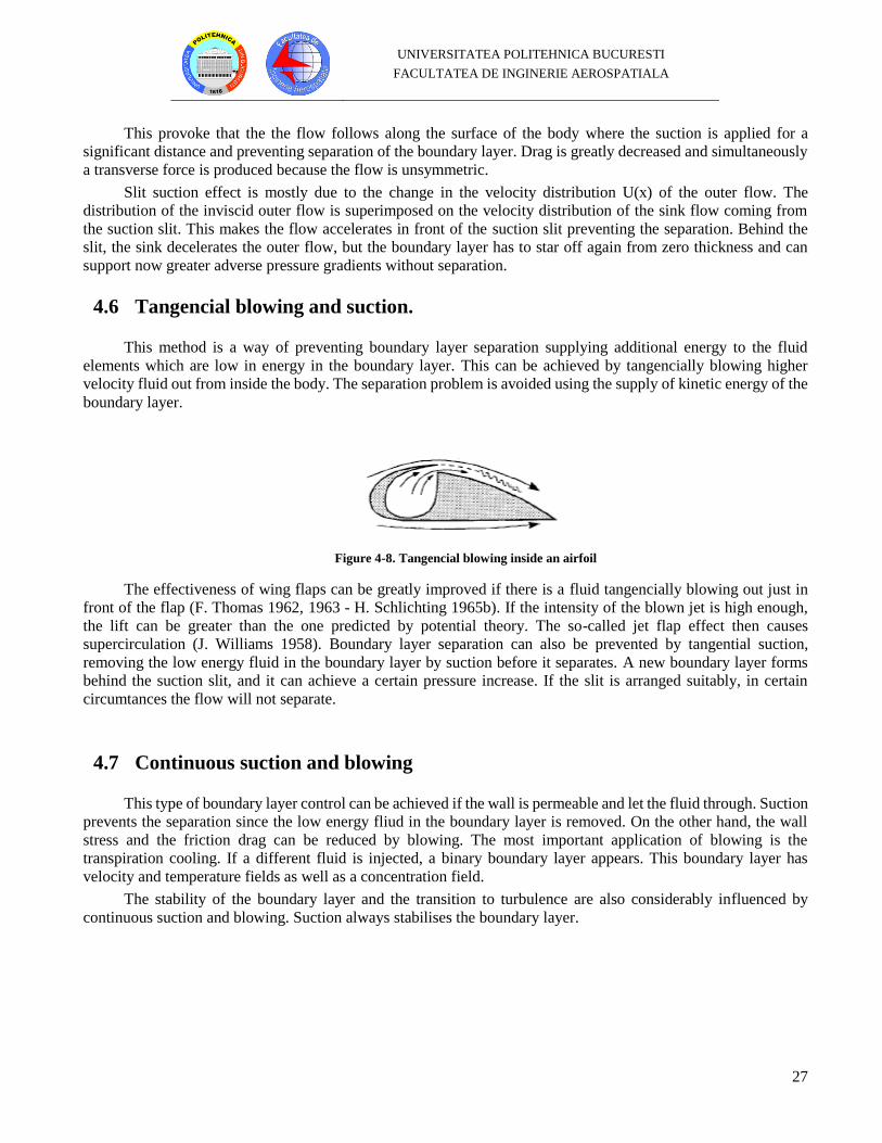
4.4 Controlling Separation by Suction
There are many cases in which control of the boundary-layer separation is important. Suction can be used
for this purpose too. If a profile equipped with suction slots is placed at a high enough angle of attack (Figure 4-6
(a)), suction will not be able to maintain the entire boundary ayer in the laminar state. It can, however, exert a
profound effect upon the turbulent layer, frequently keeping the flow attached well beyond the angle at which
stalling occurs without suction (Figure 4-6 (b)). In general, more suction power is required to attach the flow that
is already stalled than to maintain attached flow at the same angle of attack.
Separation control by suction is accomplished by drawing the low-momentum layers from the bottom of the
boundary layer intro the suction slots. This draws the higher-energy air from the outer layers closer to the surface.
4.5 Slit Suction
This type of controlling the boundary layer was first studied by Prandtl (1904), he achieved some surprinsing
effects. In Figure 4-7 a flow past through a circular cylinder where suction is applied through one side slit.
Figure 4-7. Circular cylinder with a slit suction inside a fluid flow
Figure 4-6. Multi-slotted profile of Figure 4-5 at high angle of attack. (a) Suction on. Separation is
prevented. (b) No suction. Flow totally separates from the upper surfaces.
UNIVERSITATEA POLITEHNICA BUCURESTI
FACULTATEA DE INGINERIE AEROSPATIALA
27
This provoke that the the flow follows along the surface of the body where the suction is applied for a
significant distance and preventing separation of the boundary layer. Drag is greatly decreased and simultaneously
a transverse force is produced because the flow is unsymmetric.
Slit suction effect is mostly due to the change in the velocity distribution U(x) of the outer flow. The
distribution of the inviscid outer flow is superimposed on the velocity distribution of the sink flow coming from
the suction slit. This makes the flow accelerates in front of the suction slit preventing the separation. Behind the
slit, the sink decelerates the outer flow, but the boundary layer has to star off again from zero thickness and can
support now greater adverse pressure gradients without separation.
4.6 Tangencial blowing and suction.
This method is a way of preventing boundary layer separation supplying additional energy to the fluid
elements which are low in energy in the boundary layer. This can be achieved by tangencially blowing higher
velocity fluid out from inside the body. The separation problem is avoided using the supply of kinetic energy of the
boundary layer.
Figure 4-8. Tangencial blowing inside an airfoil
The effectiveness of wing flaps can be greatly improved if there is a fluid tangencially blowing out just in
front of the flap (F. Thomas 1962, 1963 - H. Schlichting 1965b). If the intensity of the blown jet is high enough,
the lift can be greater than the one predicted by potential theory. The so-called jet flap effect then causes
supercirculation (J. Williams 1958). Boundary layer separation can also be prevented by tangential suction,
removing the low energy fluid in the boundary layer by suction before it separates. A new boundary layer forms
behind the suction slit, and it can achieve a certain pressure increase. If the slit is arranged suitably, in certain
circumtances the flow will not separate.
4.7 Continuous suction and blowing
This type of boundary layer control can be achieved if the wall is permeable and let the fluid through. Suction
prevents the separation since the low energy fliud in the boundary layer is removed. On the other hand, the wall
stress and the friction drag can be reduced by blowing. The most important application of blowing is the
transpiration cooling. If a different fluid is injected, a binary boundary layer appears. This boundary layer has
velocity and temperature fields as well as a concentration field.
The stability of the boundary layer and the transition to turbulence are also considerably influenced by
continuous suction and blowing. Suction always stabilises the boundary layer.
UNIVERSITATEA POLITEHNICA BUCURESTI
FACULTATEA DE INGINERIE AEROSPATIALA
28
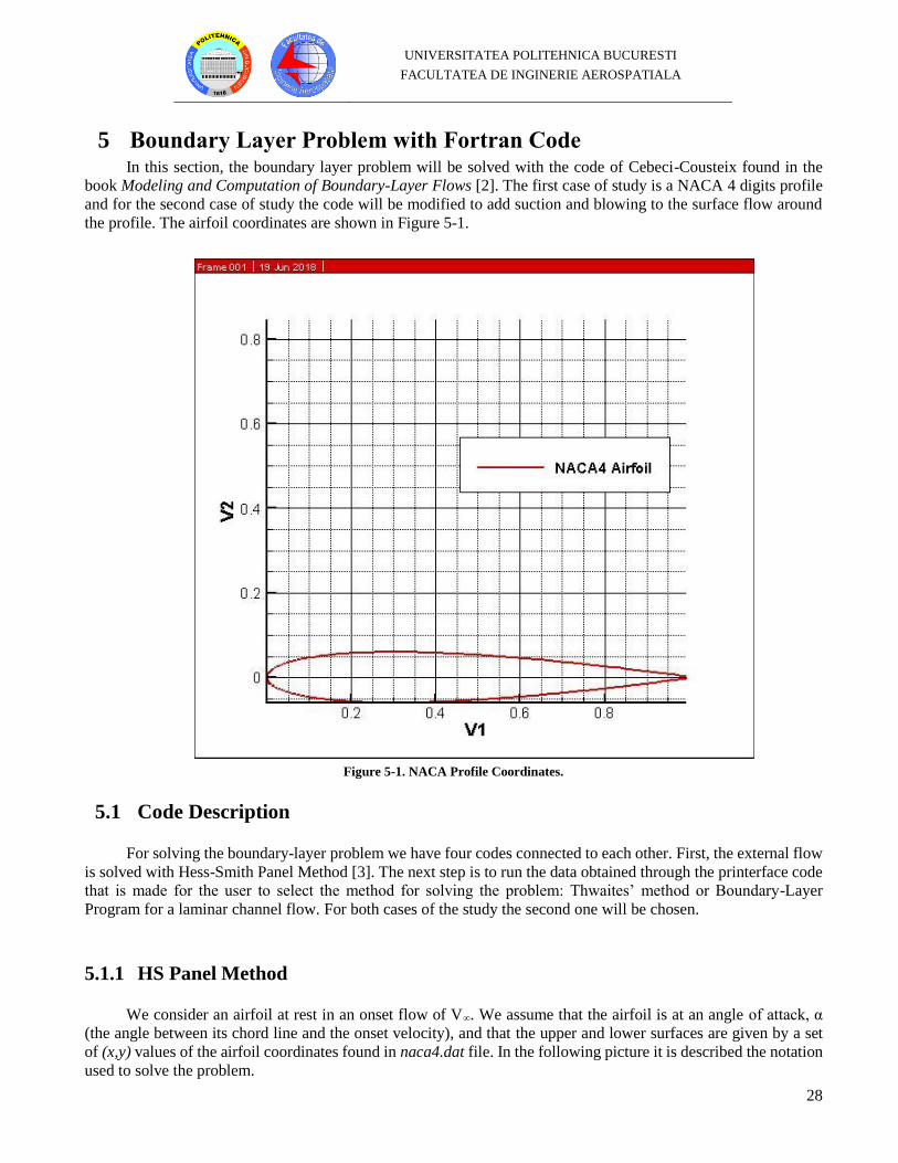
5 Boundary Layer Problem with Fortran Code In this section, the boundary layer problem will be solved with the code of Cebeci-Cousteix found in the
book Modeling and Computation of Boundary-Layer Flows [2]. The first case of study is a NACA 4 digits profile
and for the second case of study the code will be modified to add suction and blowing to the surface flow around
the profile. The airfoil coordinates are shown in Figure 5-1.
Figure 5-1. NACA Profile Coordinates.
5.1 Code Description
For solving the boundary-layer problem we have four codes connected to each other. First, the external flow
is solved with Hess-Smith Panel Method [3]. The next step is to run the data obtained through the printerface code
that is made for the user to select the method for solving the problem: Thwaites’ method or Boundary-Layer
Program for a laminar channel flow. For both cases of the study the second one will be chosen.
5.1.1 HS Panel Method
We consider an airfoil at rest in an onset flow of V∞. We assume that the airfoil is at an angle of attack, α
(the angle between its chord line and the onset velocity), and that the upper and lower surfaces are given by a set
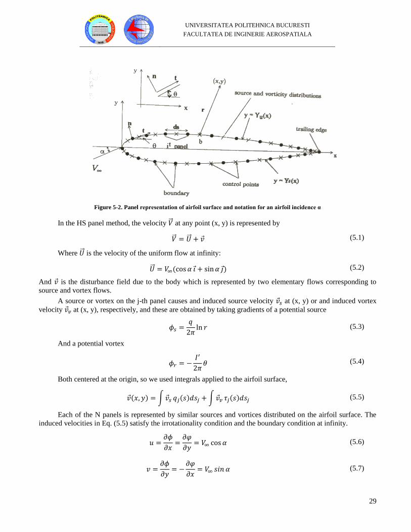
of (x,y) values of the airfoil coordinates found in naca4.dat file. In the following picture it is described the notation
used to solve the problem.
UNIVERSITATEA POLITEHNICA BUCURESTI
FACULTATEA DE INGINERIE AEROSPATIALA
29
Figure 5-2. Panel representation of airfoil surface and notation for an airfoil incidence α
In the HS panel method, the velocity �⃗� at any point (x, y) is represented by
�⃗� = �⃗⃗� + 𝑣 (5.1)
Where �⃗⃗� is the velocity of the uniform flow at infinity:
�⃗⃗� = 𝑉∞(cos𝛼 𝑖 + sin𝛼 𝑗 ) (5.2)
And 𝑣 is the disturbance field due to the body which is represented by two elementary flows corresponding to
source and vortex flows.
A source or vortex on the j-th panel causes and induced source velocity 𝑣 𝑠 at (x, y) or and induced vortex
velocity 𝑣 𝑣 at (x, y), respectively, and these are obtained by taking gradients of a potential source
𝜙𝑠 =𝑞
2𝜋ln 𝑟 (5.3)
And a potential vortex
𝜙𝑟 = −𝐼′
2𝜋𝜃 (5.4)
Both centered at the origin, so we used integrals applied to the airfoil surface,
𝑣 (𝑥, 𝑦) = ∫𝑣 𝑠 𝑞𝑗(𝑠)𝑑𝑠𝑗 + ∫𝑣 𝑣 𝜏𝑗(𝑠)𝑑𝑠𝑗 (5.5)
Each of the N panels is represented by similar sources and vortices distributed on the airfoil surface. The
induced velocities in Eq. (5.5) satisfy the irrotationality condition and the boundary condition at infinity.
𝑢 =𝜕𝜙
𝜕𝑥=
𝜕𝜑
𝜕𝑦= 𝑉∞ cos 𝛼 (5.6)
𝑣 =𝜕𝜙
𝜕𝑦= −
𝜕𝜑
𝜕𝑥= 𝑉∞ 𝑠𝑖𝑛 𝛼 (5.7)
UNIVERSITATEA POLITEHNICA BUCURESTI
FACULTATEA DE INGINERIE AEROSPATIALA
30
For uniqueness of the solutions, it is also necessary to specify the magnitude of the circulation around the
body. To satisfy the boundary conditions on the body, which correspond to the requirement that the surface of the
body is a streamline o the flow, that is,
𝜑 = 𝑐𝑜𝑛𝑠𝑡𝑎𝑛𝑡 or 𝜕𝜙
𝜕𝑛= 0 (5.8)
At the surface on which n is the direction of the normal, the sum of the source-induced and vorticity-induced
velocities and freestream velocity is set to zero in the normal direction to the surface of each of the N panels. If the
tangential and normal components of the total velocity at the control point of the i-th panel denoted by (𝑉𝑡)𝑖 and (𝑉𝑛)𝑖, the flow tangency conditions are then satisfied at panel control points by requiring that the resultant velocity
at each control point has only (𝑉𝑡)𝑖 and
(𝑉𝑛)𝑖 = 0 𝑖 = 1,2,… ,𝑁 (5.9)
Thus, to solve the Laplace equation with this approach, at the i-th panel control point we compute the normal
(𝑉𝑛)𝑖 and the tangential (𝑉𝑡)𝑖 velocity components onduced by the source and vorticity distributions on all panels
including the i-th itself, and separately sum all the induced velocities for the normal and tangential components
together with the freesstream velocity components. The resulting expressions, which satisfy the irrotationality
condition, must also satisfy the boundary conditions discussed above. Before discussing this aspect of the problem,
it is convenient to write Eq. (5.1) expressed in terms of its velocity components by
(𝑉𝑛)𝑖 = ∑𝐴𝑖𝑗𝑛 𝑞𝑗
𝑁
𝑗=1
+ ∑𝐵𝑖𝑗𝑛𝜏𝑗
𝑁
𝑗=1
+ 𝑉∞ sin(𝛼 − 𝜃𝑖) (5.10)
(𝑉𝑡)𝑖 = ∑𝐴𝑖𝑗𝑡 𝑞𝑗
𝑁
𝑗=1
+ ∑𝐵𝑖𝑗𝑡 𝜏𝑗
𝑁
𝑗=1
+ 𝑉∞ cos(𝛼 − 𝜃𝑖) (5.11)
Where 𝐴𝑖𝑗𝑛 , 𝐴𝑖𝑗
𝑡 , 𝐵𝑖𝑗𝑛 , 𝐵𝑖𝑗
𝑡 are known as influence coefficients, defined as the velocities induced at a control
point (𝑥𝑚𝑖, 𝑦𝑚𝑖). More specifically, 𝐴𝑖𝑗𝑛 and 𝐴𝑖𝑗
𝑡 denote the normal and tangential velocity components,
respectively, induced at the i-th panel control point by a unit strength source vdistribution on th j-th panel, and 𝐵𝑖𝑗𝑛
and 𝐵𝑖𝑗𝑡 are those induced by a unit of strength vorticity distribution on th j-th. The influence coefficients are related
to eh airfoil geometry and the panel arrangement. The expression that define the matrices are given and calculated
in the code in the subroutine COEF (sinalf, cosalf).
For smooth bodies such as ellipse, the problem of rationally determining the circulation has yet to be solved.
Such bodies have circulation associated with them, and resulting lift forces, but there is no rule for calculating these
forces. If, on the other hand, we deal with an airfoil having a sharp trailing edge, we can apply the Kutta condition.
It turns out that for every value of circulation except one, the inviscid velocity is infinite at the trailing edge. The
Kutta condition states that the particular value of circulation that gives a finite velocity at the trailing edge is the
proper one to choose. This condition does not include bodies with nonsharp trailing edges and bodies on which the
viscous effects have been simulated by, for example, surface blowing.
In the panel method, the Kutta condition is indirectly applied by deducing another property of the flow at the
trailing edge that is a direct consequence of the finiteness of the velocity. This property is used as the “Kutta
condition” and it involve the following:
a. A streamline of the flow leaves the trailing edge along the bisector of the trailing-edge angle.
b. Upper and lower displacement total velocities approach a common limit at the trailing edge. The limiting
value is zero if the trailing-edge angle is non-zero.
c. Source and/or vorticity strengths at the trailing edge must satisfy conditions to allow finite velocity.
UNIVERSITATEA POLITEHNICA BUCURESTI
FACULTATEA DE INGINERIE AEROSPATIALA
31
Of the above, property (b) is more widely used. At first, it may be thought that this property requires setting
bth the upper and lower surface velocities equal to zero. This gives two conditions, which cannot be satisfied by
adjusting a single parameter. The most reasonable choice is to make these two total velocities in the downstream
direction at the 1st and N-th panel control points equal so that the flow leaves the trailing edge smoothly. Since the
normal velocity on the surface is zero according to Eq. (5.9), the magnitudes of the two tangential velocities at the
trailing edge must be equal, that is,
(𝑉𝑡)𝑁 = −(𝑉𝑡)1 (5.12)
Introducing the flow tangency condition, Eq. (5.9) into Eq. (5.10) and noting that 𝜏𝑗 = 𝜏, we get
∑𝐴𝑖𝑗𝑛 𝑞𝑗
𝑁
𝑗=1
+ 𝜏∑𝐵𝑖𝑗𝑛
𝑁
𝑗=1
+ 𝑉∞ sin(𝛼 − 𝜃𝑖) = 0, 𝑖 = 1,2,… ,𝑁 (5.13)
In terms of the unknows, 𝑞𝑗 (𝑗 = 1,2, … ,𝑁) and 𝜏, the Kutta condition of Eq. (5.12) and Eq. (5.13) for a
system of algebraic equation which can be written in the following form:
𝐴𝑥 = 𝑏 (5.14)
Here, A is a square matrix of order (N+1) and 𝑥 = (𝑞1, … , 𝑞𝑖, … , 𝑞𝑁 , 𝜏)𝑇 and 𝑏 = (𝑏1, … , 𝑏𝑖, … , 𝑏𝑁, 𝑏𝑁+1)𝑇.
First, the elements of 𝑎𝑖𝑗 are determined by the following equations:
𝑎𝑖𝑗 = 𝐴𝑖𝑗𝑁 , (𝑖, 𝑗) = 1,2, … ,𝑁 (5.15)
𝑎𝑖,𝑁+1 = ∑𝐵𝑖𝑗𝑛
𝑁
𝑗=1
, 𝑖 = 1,2,… ,𝑁 (5.16)
𝑎𝑁+1,𝑗 = 𝐴1𝑗𝑡 + 𝐴𝑁𝑗
𝑡 , 𝑗 = 1,2,… ,𝑁 (5.17)
𝑎𝑁+1,𝑁+1 = ∑(𝐵1𝑗𝑡 + 𝐵𝑁𝑗
𝑡 )
𝑁
𝑗=1
(5.18)
And the elements of �⃗� are solved with,
𝑏𝑖 = −𝑉∞ sin(𝛼 − 𝜃𝑖) , 𝑖 = 1,2, … ,𝑁 (5.19)
𝑏𝑁−1 = −𝑉∞ cos(𝛼 − 𝜃1) − 𝑉∞ cos(𝛼 − 𝜃𝑁) (5.20)
So that, the solution of Eq. (5.14) can be obtained by the Gaussian elimination method, which is calculated
in the GAUSS (1) subroutine of the panel.f code.
Once 𝑥 is determined by GAUSS subroutine so that source strengths 𝑞𝑖 (𝑖 = 1,2,… ,𝑁) and vorticity 𝜏 on
the airfoil surface are known, the tangential velocity component (𝑉𝑡)𝑖 at each control point can be calculated with
VPDIS subroutine. Denoting 𝑞𝑖 with 𝑄(𝐼) and 𝜏 with GAMMA, the tangential velocities (𝑉𝑡)𝑖 are obtained with
the help of Eq. (5.11). The subroutine also determines the dimensionless pressure coefficient 𝐶𝑃.
UNIVERSITATEA POLITEHNICA BUCURESTI
FACULTATEA DE INGINERIE AEROSPATIALA
32
To sum up, the code is divided in four main subroutines:
• COEF (SINALF, COSALF): in this subroutine the elements 𝑎𝑖𝑗 of the matrix A and the elements
of �⃗� are calculated. We note that N+1 corresponds to KUTTA, and N to NODTOT.
• GAUSS (1): the solution of Eq. (5.14) is obtained with the Gauss elimination method.
• VPDIS (SINALF, COSALF): it calculates the tangential velocity component (𝑉𝑡)𝑖 and the
dimensionless pressure coefficient 𝐶𝑃.
• CLCM (SINALF, COSALF): the dimensionless pressure in the appropriate directions is integrated
to compute the aerodynamic force and the coefficient for lift (CL) and pitching moment (CM)
about the leading edge of the airfoil.
5.1.2 Printerface code
The purpose of this code is to choose the conditions and solver for the boundary-layer problem. It is
customary to select the type of flow or the type of method, but for our problem we will choose laminar flow and
differential method.
The main parameters and options are the following:
• IFLOW: 0 – for laminar flow, 1 – for laminar and turbulent flow or 2 – for only turbulent flow.
• BIGL: is the reference length that we must choose.
• UREF: is the reference velocity that needs to be selected.
• CNU: is the kinematic viscosity of the flow of study.
• RL: the program calculates the Reynolds’ number of the flow.
• Method: 0 – differential (blp2d.f or stp2d.f), 1 – integral (Thwaites’ or Head’s method).
• IGEOMETRY: this value will provide the program the format of the input data; 0 – panel method
or 1 – input [ x (I) s (I) Ue (I)].
• Isurface: 0 – lower surface or 1 – upper surface.
• P2: is the dimensionless pressure gradient; 1 – airfoil or 0 – flat plate.
Once all options are chosen, the program calculates points and velocities of the control points for the surface
chosen. After this, the distance from the initial point is computed and it generates the input data for the solver.
5.1.3 BLP2D code
This program solves the boundary-layer problem by differential method for two-dimensional flows for
obtaining the solutions of the continuity and momentum equations for laminar and turbulent external flows with
boundary conditions. BLP2D employs numerical methods for solving the problem and with proper modifications
it can also be used for free-shear layer flows and also for internal flows.
In BLP2, the calculation starts at the leading edge, 𝑥 = 0, where the flow is laminar and becomes turbulent
at any x-location by specifying the transition location. The program, however, is general and can be modified to
include the cases where the calculations start as either laminar or turbulent at a specified x-location.
The solution procedure requires the specification of the dimensionless pressure gradient 𝑚(𝑥) and the mass
transfer 𝑓𝑤(𝑥) parameters. These two quantities can be obtained from their definitions and the specified reference
Reynolds number 𝑅𝐿 and the dimensionless external and mass-transfer velocities, 𝑢𝑒(𝑥) and 𝑣𝑤(𝑥) respectively.
UNIVERSITATEA POLITEHNICA BUCURESTI
FACULTATEA DE INGINERIE AEROSPATIALA
33
The solution procedure also requires the generation of a grid nirmal to the surface, η-grid, and along the
surface, x-grid. The latter requirement is usually satisfied by specifying locations with intervals which can be
uniform or nonuniform. Its distribution depends on the variation of 𝑢𝑒 with 𝑥 so that the pressure gradient parameter
𝑚(𝑥) can be calculated accurately. To ensure this requirement, it is necessary to take small ∆𝑥 steps (𝑘𝑛) where
there are rapid variations in 𝑢𝑒(𝑥) and where flow approaches separation.
For laminar flows, it is often sufficient to use a uniform grid in the η-direction. For turbulent flows, however,
a uniform grid is not satisfactory because the boundary-layer thickness 𝜂𝑒 and dimensionless wall shear parameter
𝑓𝑤′′ are much larger in turbulent flows than laminar flows. Since short steps in η must be taken to maintain
computational accuracy when 𝑓𝑤′′ is large, the steps near the wall in a turbulent boundary-layer must be shorter
than the corresponding steps in a laminar boundary-layer under similar conditions.
BLP2 consists of a MAIN routine, which contains the logic of computations, and seven subroutines: INPUT,
IVPL, GROWTH, EDDY, CMOM, SOLV3 and OUTPUT. The following subsections describe the function of
each subroutine except EDDY.
• MAIN
BLP2 solves the linearized for of the equations. Through an iterative process, the solution of the equations
is obtained for successive estimates of the velocity profiles is needed with subsequent need to check the
convergence of the solutions. A convergence criterion based on 𝑣0 which corresponds to 𝑓𝑤′′ is usually used
and the iterations, which are generally quadratic for laminar flows, are sttoped when
|𝛿𝑣0(= 𝐷𝐸𝐿𝑉(1))| < 𝜖1 (5.21)
With 𝜖1 taken as 10−5. For turbulent flows, due to the approximate linearization procedure used for the
turbulent diffusion term, the rate of convergence is not quadratic, and solutions are usually acceptable when
the ratio of |𝛿𝑣0/𝑣0| is less than 0.02. With proper linearization, quadratic convergence of the solutions can
be obtained.
After the convergence of the solutions, the OUTPUT subroutine is called and the profiles F, U, V and B,
which represent the variables 𝑓𝑗, 𝑢𝑗, 𝑣𝑗 and 𝑏𝑗 are shifted.
• Subroutine INPUT
In this subroutine we generate the η-grid, compute 𝛾𝑡𝑟 for the transition region, calculate the pressure
gradient parameters 𝑚 and 𝑚1 and specify 𝜂𝑒 at 𝑥 = 0 and the reference Reynolds number 𝑅𝐿.
In addition, the following data are read in and the total number of j-points (NP) is computed.
- NXT, total number of x-stations, not to exceed 60.
- NTR, NX-station for transition location 𝑥𝑡𝑟
- NPT, total number of η-grid points
- DETA(1), ∆𝑛-initial step size of the variable grid system. Use ∆𝑛 = 0.01 for turbulent flows. If
desired, it may be changed.
- ETAE, transformed boundary-layer thickness, 𝜂𝑒
- VGP, K is the variable-grid parameter. Use 𝐾 = 1.0 for laminar flow and 𝐾 = 1.14 for turbulent flow.
For a flow consisting of both laminar and turbulent flows, use 𝐾 = 1.14.
- RL, Reynolds number
- x, surface distance, feet or meters, or dimensionless
- 𝒖𝒆, velocity, feet per second or meter per second, or dimensionless
UNIVERSITATEA POLITEHNICA BUCURESTI
FACULTATEA DE INGINERIE AEROSPATIALA
34
The calculation of 𝑚 is achieved from the given external velocity distribution 𝑢𝑒(𝑥) and from the definition
of 𝑚 (≡ 𝑃2) except for the first NX-station where P2(1) is read in. The derivative of 𝑑𝑢𝑒/𝑑𝑥 (DUDS) is
obtained by using three-point Lagrange interpolation formulas given by (𝑛 < 𝑁):
(𝑑𝑢𝑒
𝑑𝑥)𝑛
= −𝑢𝑒
𝑛−1
𝐴1(𝑥𝑛+1 − 𝑥𝑛) +
𝑢𝑒𝑛
𝐴2(𝑥𝑛+1 − 2𝑥𝑛 + 𝑥𝑛−1) +
𝑢𝑒𝑛+1
𝐴3(𝑥𝑛 − 𝑥𝑛−1) (5.22)
Here N refers to the last 𝑥𝑛 station and
𝐴1 = (𝑥𝑛 − 𝑥𝑛−1)(𝑥𝑛+1 − 𝑥𝑛−1)
𝐴2 = (𝑥𝑛 − 𝑥𝑛−1)(𝑥𝑛+1 − 𝑥𝑛)
𝐴3 = (𝑥𝑛+1 − 𝑥𝑛)(𝑥𝑛+1 − 𝑥𝑛−1)
(5.23)
The derivative of 𝑑𝑢𝑒/𝑑𝑥 at the end point 𝑛 = 𝑁 is given by
(𝑑𝑢𝑒
𝑑𝑥)𝑁
= −𝑢𝑒
𝑁−2
𝐴1(𝑥𝑁 − 𝑥𝑁−1) +
𝑢𝑒𝑁−1
𝐴2(𝑥𝑁 − 𝑥𝑁−2) +
𝑢𝑒𝑁
𝐴3(2𝑥𝑁 − 𝑥𝑁−2 − 𝑥𝑁−1) (5.24)
Where now
𝐴1 = (𝑥𝑁−1 − 𝑥𝑁−2)(𝑥𝑁 − 𝑥𝑁−2)
𝐴2 = (𝑥𝑁−1 − 𝑥𝑁−2)(𝑥𝑁 − 𝑥𝑁−1)
𝐴3 = (𝑥𝑁 − 𝑥𝑁−1)(𝑥𝑁 − 𝑥𝑁−2)
(5.25)
• Subroutine IVPL
Since the equations are solved in linearized from, initial stimates of 𝑓𝑗, 𝑢𝑗 and 𝑣𝑗 are needed in order to obtain
the solutions of the nonlinear Falkner-Skan equation. Various expressions can be used for this purpose. Since
Newton’s method is used, however, it it useful to provide as good estimate as is possible and an expression of the
form.
𝑢𝑗 =3
2
𝜂𝑗
𝜂𝑒−
1
2(𝜂𝑗
𝜂𝑒)3 (5.26)
Usually satisfies this requirement. The above equation is obtained by assuming a third-order polynomial of
the form
𝑓′ = 𝑎 + 𝑏𝜂 + 𝑐𝜂3 (5.27)
And by determining constants a, b, c, from the boundary conditions for the zero-mass transfer case and from
one of the properties of momentum equation which requires that 𝑓′′ = 0 at 𝜂 = 𝜂𝑒.
The other profiles 𝑓𝑗, 𝑣𝑗 can be written as
𝑓𝑗 =𝜂𝑒
4(𝜂𝑗
𝜂𝑒)2
[3 −1
2(𝜂𝑗
𝜂𝑒)2
] (5.28)
𝑣𝑗 =3
2
1
𝜂𝑒[1 − (
𝜂𝑗
𝜂𝑒)2
] (5.29)
UNIVERSITATEA POLITEHNICA BUCURESTI
FACULTATEA DE INGINERIE AEROSPATIALA
35
• Subroutine COEF3
This is one of the most important subroutines of BLP. It defines the coefficients of the linearized momentum
equation.
• Subroutine SOLV3
This subroutine uses the block-elimination method determining expressions such as ∆𝑗, Γ𝑗, �⃗⃗� 𝑗 and 𝛿 𝑗. Noting
that the Γ𝑗 matrix has the same structure as B𝑗 and denoting the elements of γ𝑗, by γ𝑖𝑘 (𝑖, 𝑘 = 1, 2, 3), we can write
Γ𝑗 as
Γ𝑗 ≡ |
(𝛾11)𝑗 (𝛾12)𝑗 (𝛾13)𝑗(𝛾21)𝑗 (𝛾22)𝑗 (𝛾23)𝑗
0 0 0
| (5.30)
Similarly, if the elements of ∆𝑗 are denoted by 𝛼𝑖𝑘 we can write ∆𝑗 as
∆𝑗 ≡ |
(𝛼11)𝑗 (𝛼12)𝑗 (𝛼13)𝑗(𝛼21)𝑗 (𝛼22)𝑗 (𝛼23)𝑗
0 −1 −ℎ𝑗+1
2
| 0 ≤ 𝑗 ≤ 𝐽 − 1 (5.31)
And for 𝑗 = 𝐽 the elements of the third row, which correspond to the boundary conditions, are (0, 1, 0).
For 𝑗 = 0, ∆0 = 𝐴0; therefore the values of (𝛼𝑖𝑘)0 are
(𝛼11)0 = 1 (𝛼12)0 = 0 (𝛼13)0 = 0(𝛼21)0 = 0 (𝛼22)0 = 1 (𝛼23)0 = 0
(5.32)
All the rest of the parameters are calculated with the expressions given in [3] pages 119 and 120. The
subroutine SOLV3 makes use of these formulas to obtain the results.
• Subroutine OUTPUT
This subroutine prints out the desired profiles such as 𝑓𝑗, 𝑢𝑗, 𝑣𝑗, and 𝑏𝑗 as functions of 𝜂𝑗. It also computes
the boundary-layer parameters, 𝑐𝑓, 𝛿∗, 𝜃 and 𝑅𝑥. The calculation is made by the trapezoidal rule.
UNIVERSITATEA POLITEHNICA BUCURESTI
FACULTATEA DE INGINERIE AEROSPATIALA
36
5.2 1st Case: The Influence of the 𝒗𝒘
This study is made to obtain the results of the boundary-layer parameters with the cases of suction and
injection. The code was modified to have into account the suction/injection velocity in some stations of the surface
profile. The program provides us the pressure gradient in order to choose the correct sequence of stations where
the suction or injection velocity will be effective.
The blowing case is going to be studied in the 4th case. For a laminar flow, to blow some fluid in the surface
doesn’t provide any improvement because the boundary layer separates at the same point of the original airfoil
without blowing or suction. For turbulent flows, blowing appears to be effective for the boundary layer because it
causes attachement in thr boundary layer at the beginning of it and continues downstream.
5.3 2nd Case: Study of the Optimum Section
In this case, the optimum section for the case of suction is studied. The aim is to obtain the best configuration
of the profile with a suction velocity chosen and comparing with other sections. The injection case is rejected due
to the results obtained for the 1st case; these results show how suction provide better results and the boundary layer
remains more attached rather than with injection.
5.4 3rd Case: Value of 𝒗𝒘
Once we have the results from the other two cases, it is interesting to know which the best value for the
suction velocity is, and this value will provide the best results. This is studied through the friction coefficient,
because is one of the most important parameters of the boundary layer in an airfoil.
5.5 4th Case: Influence of the Turbulence
For this case, the code was changed to solve with k-epsilon model and to obtain the results for the blowing
case. K-epsilon turbulence model is a two-equation model which gives a general description of turbulence by means
of two transport equations. The original impetus for the K-epsilon model was to improve the mixing-length model,
as well as to find an alternative to algebraically prescribing turbulent length scales in moderate to high complexity
flows. The aim is to verify if a small value of blowing in turbulent flow provides a delaying of the separation of the
boundary layer.

UNIVERSITATEA POLITEHNICA BUCURESTI
FACULTATEA DE INGINERIE AEROSPATIALA
37
6 Numerical results In this section, the results obtained for the four cases explained in 5.2, 5.3, 5.4 and 5.5 are shown and
explained to understand the behavior of the boundary layer under the effects of blowing, suction and turbulent flow.
6.1 Suction 𝒗𝒘 < 𝟎
The boundary layer for the profile chosen is not attached at certain point of the upper surface. So, to include
suction will produce a re-attachement in the upper surface of the airfoil for the same angle of attack. The parameters
studied are the following.
6.1.1 η vs u
The next figure shows the suction effect compared with the airfoil for the velocity component u versus the
adimensional parameter η for station 112 to see how the velocity profile changes over the surface. The following
stations are not calculated for the airfoil because the boundary layer is not attached at certain point of the upper
surface. The effect starts at station 107 until 180.
• Station 112
Figure 6-1. Representation of η – u for station 112.
UNIVERSITATEA POLITEHNICA BUCURESTI
FACULTATEA DE INGINERIE AEROSPATIALA
38
In Figure 6-1 it is shown how at the beginning of the surface, for the station 112 with suction the velocity u
is greater than the original airfoil without suction. This means that we can achieve a velocity gradient more stable
for the firsts station and keep the boundary layer attached from the beginning.
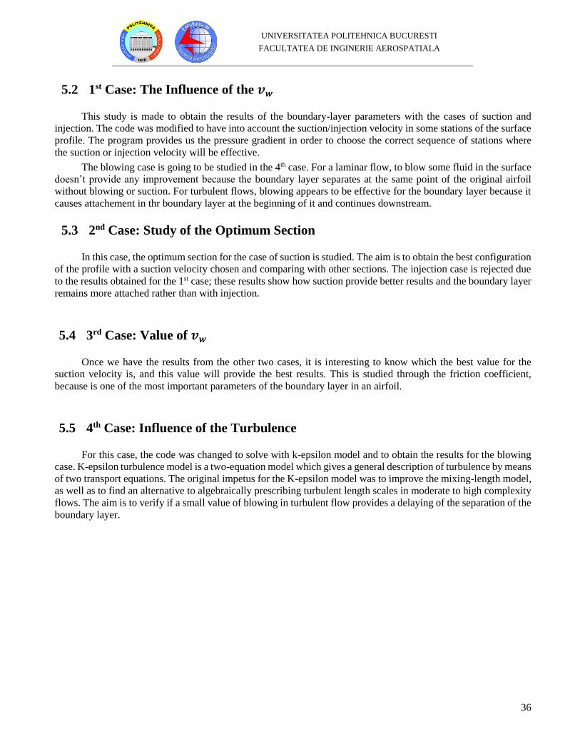
6.1.2 Cf vs x
Friction coefficient is caused by the viscosity of fluids ad its developed from laminar drag to turbulent drag
as fluid moves on the surface. For this case, it is studied to compare the differences between the original airfoil and
the suction effect.
Figure 6-2. Representation of Cf – x.
In Figure 6-2 it can be appreciated how for the original airfoil the friction coefficient has smaller values for
the beginning of the upper surface of the profile. For the suction case, the values of the friction coefficient are
higher due to this effect. It is also important the fact that for the airfoil we only have values until 0.22 approximatly
and the value is close to zero. Then the suction effect stars and the friction coefficient increase for the flow
downstream.
UNIVERSITATEA POLITEHNICA BUCURESTI
FACULTATEA DE INGINERIE AEROSPATIALA
39
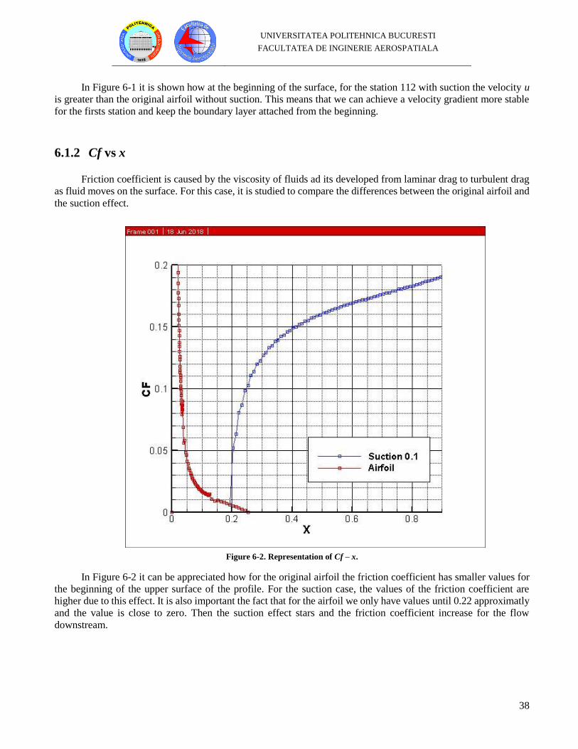
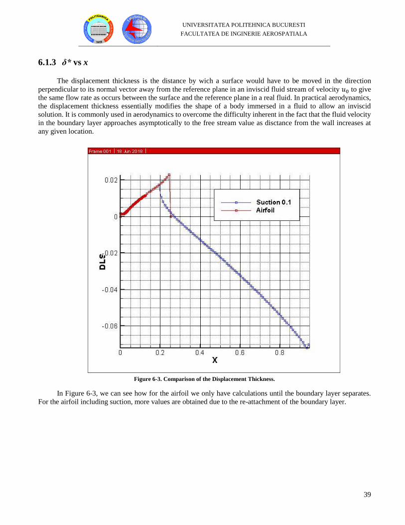
6.1.3 δ* vs x
The displacement thickness is the distance by wich a surface would have to be moved in the direction
perpendicular to its normal vector away from the reference plane in an inviscid fluid stream of velocity 𝑢0 to give
the same flow rate as occurs between the surface and the reference plane in a real fluid. In practical aerodynamics,
the displacement thickness essentially modifies the shape of a body immersed in a fluid to allow an inviscid
solution. It is commonly used in aerodynamics to overcome the difficulty inherent in the fact that the fluid velocity
in the boundary layer approaches asymptotically to the free stream value as disctance from the wall increases at
any given location.
Figure 6-3. Comparison of the Displacement Thickness.
In Figure 6-3, we can see how for the airfoil we only have calculations until the boundary layer separates.
For the airfoil including suction, more values are obtained due to the re-attachment of the boundary layer.
UNIVERSITATEA POLITEHNICA BUCURESTI
FACULTATEA DE INGINERIE AEROSPATIALA
40
6.1.4 θ vs x
The momentum thickness is the distance by which a surface would have to be moved parallel to itself towards
the reference plane in an inviscid fluid stream of velocity 𝑢0 to give the same total momentum as exists between
the surface and the reference plane in a real fluid.
Figure 6-4. Comparison of the Momentum Thickness.
Figure 6-4 shows results that are similar to the other parameters. Due to the suction applied, the boundary
layer is attached in the most part of the upper surface of the profile. It is shown how the values of the momentum
thickness increase for the airfoil and decreased for the surface where the suction is applied.
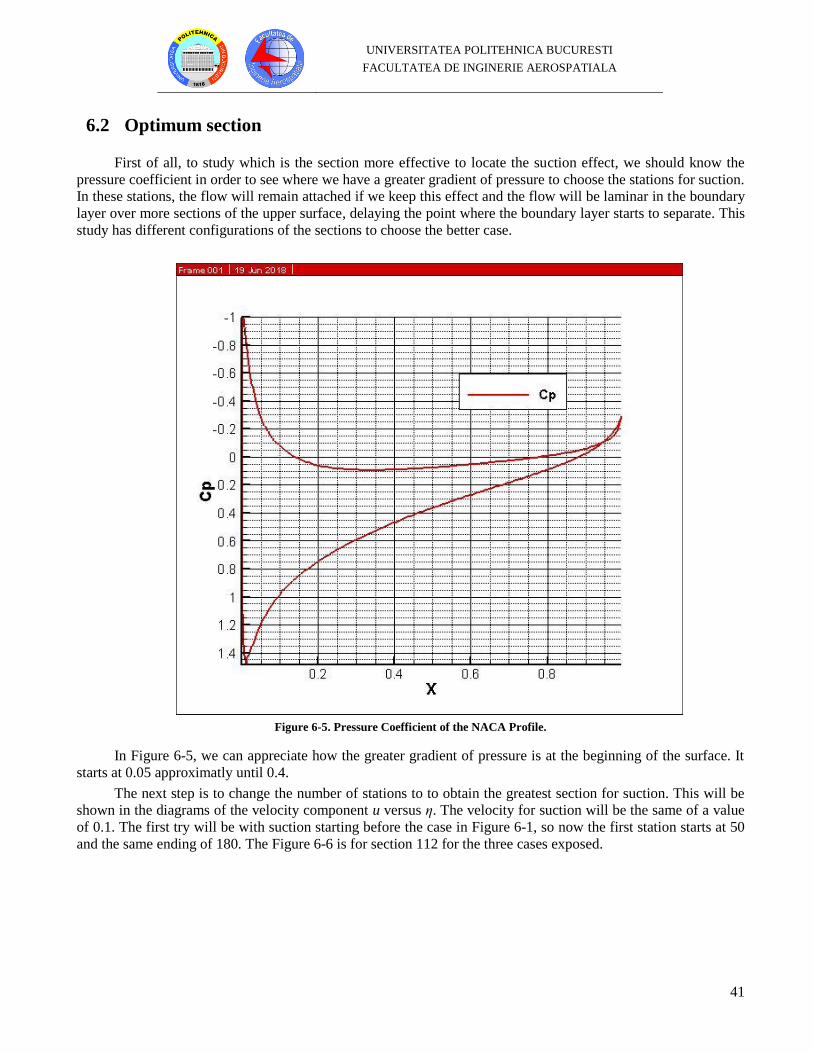
UNIVERSITATEA POLITEHNICA BUCURESTI
FACULTATEA DE INGINERIE AEROSPATIALA
41
6.2 Optimum section
First of all, to study which is the section more effective to locate the suction effect, we should know the
pressure coefficient in order to see where we have a greater gradient of pressure to choose the stations for suction.
In these stations, the flow will remain attached if we keep this effect and the flow will be laminar in the boundary
layer over more sections of the upper surface, delaying the point where the boundary layer starts to separate. This
study has different configurations of the sections to choose the better case.
Figure 6-5. Pressure Coefficient of the NACA Profile.
In Figure 6-5, we can appreciate how the greater gradient of pressure is at the beginning of the surface. It
starts at 0.05 approximatly until 0.4.
The next step is to change the number of stations to to obtain the greatest section for suction. This will be
shown in the diagrams of the velocity component u versus η. The velocity for suction will be the same of a value
of 0.1. The first try will be with suction starting before the case in Figure 6-1, so now the first station starts at 50
and the same ending of 180. The Figure 6-6 is for section 112 for the three cases exposed.
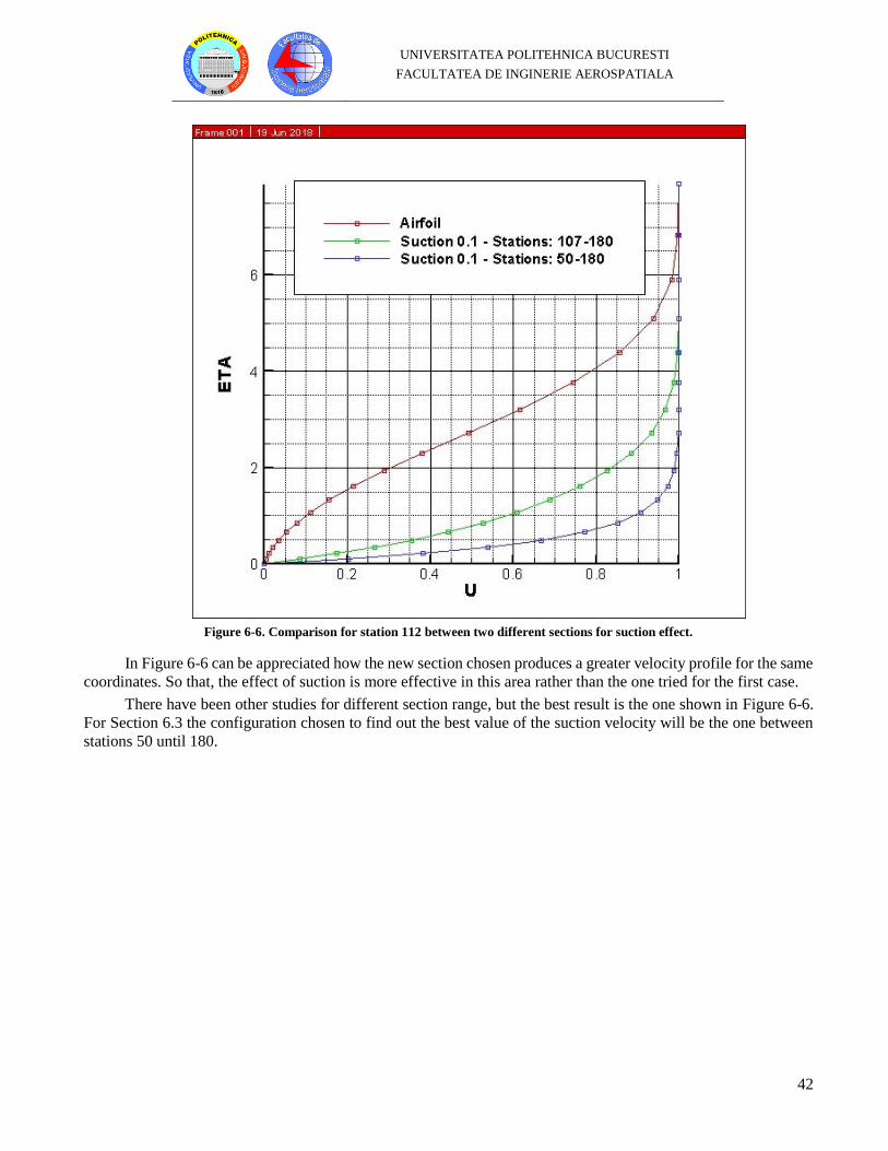
UNIVERSITATEA POLITEHNICA BUCURESTI
FACULTATEA DE INGINERIE AEROSPATIALA
42
Figure 6-6. Comparison for station 112 between two different sections for suction effect.
In Figure 6-6 can be appreciated how the new section chosen produces a greater velocity profile for the same
coordinates. So that, the effect of suction is more effective in this area rather than the one tried for the first case.
There have been other studies for different section range, but the best result is the one shown in Figure 6-6.
For Section 6.3 the configuration chosen to find out the best value of the suction velocity will be the one between
stations 50 until 180.
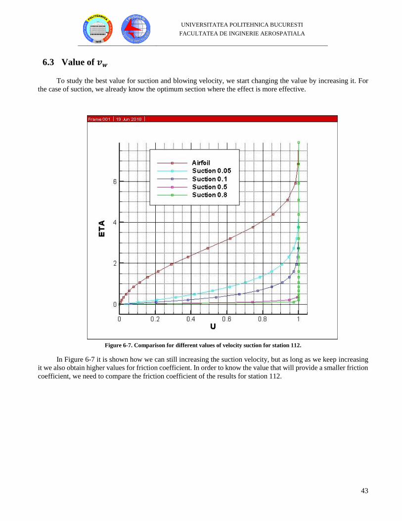
UNIVERSITATEA POLITEHNICA BUCURESTI
FACULTATEA DE INGINERIE AEROSPATIALA
43
6.3 Value of 𝒗𝒘
To study the best value for suction and blowing velocity, we start changing the value by increasing it. For
the case of suction, we already know the optimum section where the effect is more effective.
Figure 6-7. Comparison for different values of velocity suction for station 112.
In Figure 6-7 it is shown how we can still increasing the suction velocity, but as long as we keep increasing
it we also obtain higher values for friction coefficient. In order to know the value that will provide a smaller friction
coefficient, we need to compare the friction coefficient of the results for station 112.
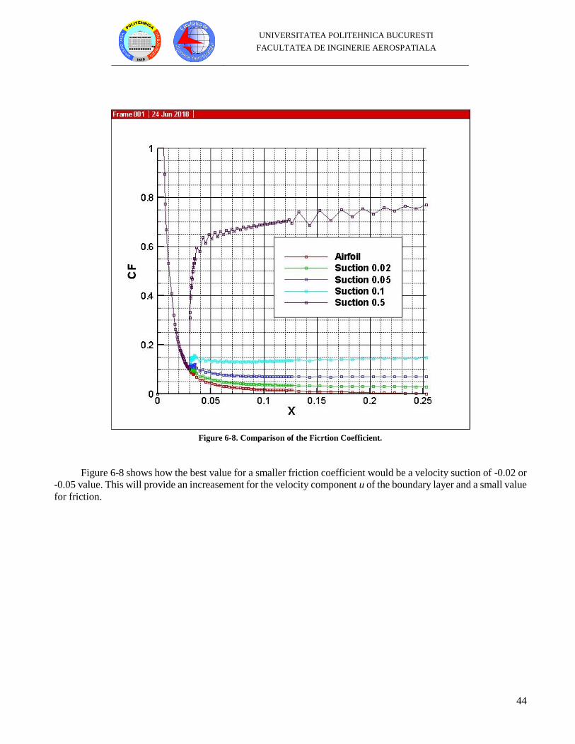
UNIVERSITATEA POLITEHNICA BUCURESTI
FACULTATEA DE INGINERIE AEROSPATIALA
44
Figure 6-8. Comparison of the Ficrtion Coefficient.
Figure 6-8 shows how the best value for a smaller friction coefficient would be a velocity suction of -0.02 or
-0.05 value. This will provide an increasement for the velocity component u of the boundary layer and a small value
for friction.
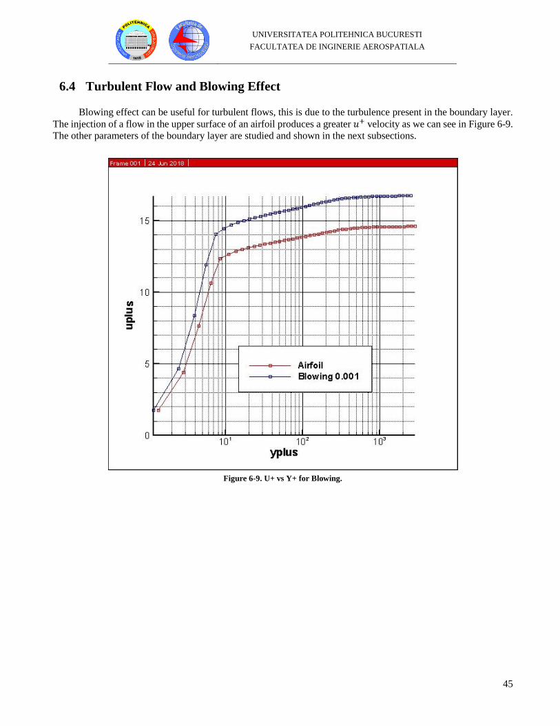
UNIVERSITATEA POLITEHNICA BUCURESTI
FACULTATEA DE INGINERIE AEROSPATIALA
45
6.4 Turbulent Flow and Blowing Effect
Blowing effect can be useful for turbulent flows, this is due to the turbulence present in the boundary layer.
The injection of a flow in the upper surface of an airfoil produces a greater 𝑢+ velocity as we can see in Figure 6-9.
The other parameters of the boundary layer are studied and shown in the next subsections.
Figure 6-9. U+ vs Y+ for Blowing.
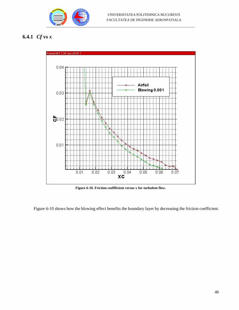
UNIVERSITATEA POLITEHNICA BUCURESTI
FACULTATEA DE INGINERIE AEROSPATIALA
46
6.4.1 Cf vs x
Figure 6-10. Friction coeffficient versus x for turbulent flow.
Figure 6-10 shows how the blowing effect benefits the boundary layer by decreasing the friction coefficient.
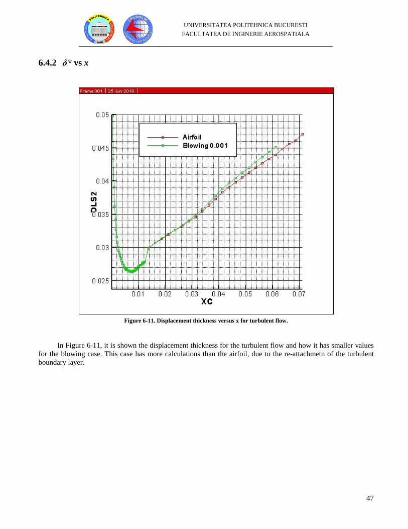
UNIVERSITATEA POLITEHNICA BUCURESTI
FACULTATEA DE INGINERIE AEROSPATIALA
47
6.4.2 δ* vs x
Figure 6-11. Displacement thickness versus x for turbulent flow.
In Figure 6-11, it is shown the displacement thickness for the turbulent flow and how it has smaller values
for the blowing case. This case has more calculations than the airfoil, due to the re-attachmetn of the turbulent
boundary layer.

UNIVERSITATEA POLITEHNICA BUCURESTI
FACULTATEA DE INGINERIE AEROSPATIALA
48
6.4.3 θ vs x
Figure 6-12. Theta versus x for turbulent flow.
In Figure 6-12 we can see how the momentum thicknes has similar values but smaller at the begginig of the
station where the effect starts to take place. It is similar to the results shown before in Figure 6-11.
UNIVERSITATEA POLITEHNICA BUCURESTI
FACULTATEA DE INGINERIE AEROSPATIALA
49
7 Conclusions The boundary layer solution for the Blasius equation was a great achievement and still is very used nowadays.
The simplest methods are useful to understand the complex problems and models. It also provides and
approximation of the solution. The aim of this research is to keep researching about the boundary layer theory in
order to determine as much information as possible of the boundary layer characteristics.
For the second part of the research, a deeper study has been carried out to calculate the main parameters of
the boundary layer with the cases of suction and blowing. It has been proved how for laminar flows it is convenient
to choose suction with a value around 0.02 and for stations starting at the begging of the surface until the end of
the surface. This produces a re-attachment in the boundary layer delaying the separation from the body.
For turbulent flows it is useful to add a small velocity blowing at the surface in order to attach the turbulent
flow in the upper surface. These results were obtained using a FORTRAN code provided from the books [2] and
[3] and modifying some parts to add the blowing and suction effect.
To conclude, it has been proved how these two effects benefits the behavior of the boundary layer under the
right conditions and it is an approach for researching in method of increasing the aerodynamic efficiency of the
airfoil.
8 References
[1] Schlichting, H., Gersten, K., “Boundary layer theory”, Germany, Springer.
[2] Cebeci, T., Cousteix, J., “Modeling and Computation of Boundary-Layer Flows”, Springer.
[3] Cebeci, T., “Turbulence Models and Their Application”, Springer.
[4] Hazen. D., “Boundary Layer Control”, National Committee for Fluid Mechanics Films.