Lakshmi Krishnamurthy v0.50 , 20 January 2014
98
1 Curve Builder in DRIP Lakshmi Krishnamurthy v0.50, 20 January 2014
Transcript of Lakshmi Krishnamurthy v0.50 , 20 January 2014

1
Curve Builder in DRIP
Lakshmi Krishnamurthy
v0.50, 20 January 2014

2
Introduction
Framework Glossary
1. Self-Jacobian: Self-Jacobian refers to the Jacobian of the Objective Function at any
point in the variate to the Objective Function at the segment nodes, i.e., ( )
( )KtY
tY
∂∂
.
2. Point-Measure State-Transform: Point-Measure transform refers to the one-to-one
transform between a state measure at a predictor ordinate and its corresponding
observation (e.g., discount factor from zero-coupon bond price observations).
3. Convolved-Measure State-Transform: Convolved-Measure transform refers to the
many-to-one transform between a state metric/predictor ordinate combination to a
given observation, i.e., a set of state metric/predictor ordinate pairs together imply an
observation (e.g., zero rates from swap fair premia).
4. Discount-Curve Native Forward Curve: For discount curves built out of instruments
dependent on forward rates, those rates and their discount curve usage ranges together
constitute the discount curve’s native forward curve range.
Overview
1. Smoothness Criterion Evolution: Smoothness formulation is related to the
minimization of strain energy (Schwarz (1989)), and the relation to Natural cubic
spline (Burden and Faires (1997)), financial cubic spline (Adams (2001)) has been
explored.
2. Empirical vs. Theoretical Curve Builder Frameworks: Zangari (1997) and Lin (2002)
discuss this in detail.
• Theoretical Term Structure posit explicit term structure for a variable known as
short rate of interest whose values are extracted, possibly, from a statistical

3
analysis of market variables (Vasicek (1977), Cox, Ingersall, and Ross (1985),
Rebonato (1998), Barzanti and Corradi (1998), Golub and Tilman (2000)).
• For bonds/treasuries see Nelson and Siegel (1987), Diament (1993), Svensson
(1994), Soderlind and Svensson (1997), Tanggaard (1997). Effectiveness of such
treatments is examined in Christensen, Diebold, and Rudebusch (2007), and
Coroneo, Nyholm, and Vidova-Koleva (2008).
• Hybrid methods use empirically determined yield curve inside of a theoretical
model (Hull and White (1990), Heath, Jarrow, and Morton (1990), Ron (2000)).
• A complete description of yield curve construction is given in Andersen and
Piterbarg (2010).
Document Layout
1. Introduction
a. Framework Glossary
b. Overview
c. Document Layout
2. Desired Curve Builder Features
a. For Discount Curves
b. For Forward Curves
c. For Credit Curves
3. Curve Construction Methodology
a. Base Methodology
b. State Span Design Components
c. Curve Calibration From Instruments/Quotes
d. Calibration Considerations
4. Curve Construction Formulation
a. Linearized Discount Curve Calibration From Instruments
b. Segment-Linear Discount Curve Calibration From Instruments
c. Curve Jacobian

4
5. Spanning Splines
a. Formulation and Setup
b. Challenges withy the Spanning Spline Approach
6. Monotone Decreasing Splines
a. Motivation
b. Exponential Rational Basis Spline Set
c. Exponential Mixture Basis Spline Set
7. Hagan West (2006) Smoothness Preserving Spanning Spline
a. Monotonicity/Convexity Preserving Estimator
b. Positivity Preserving Estimator
c. Ameliorating Estimator
d. Harmonic Spline Extension to the Framework Above
e. Minimal Quadratic Estimator
8. Penalizing Closeness of Fit and Curvature Penalty
9. Extrapolation in Curve Construction
10. Multi-Pass Curve Construction
a. Motivation
b. Bear-Sterns Multi-Pass Curve Building Techniques
11. Transition Spline (or Stitching Spline)
a. Motivation
b. Stretch Modeling using Transition Splines
c. Stretch Partition/Isolation in Transition Splines
d. Knot Insertion vs. Transition Splines
e. Overlapping Stretches
12. Index/Tenor Basis Swaps
a. Component Layout and Motivation
b. Formulation
13. Multi-Stretch Merged Curve Construction
a. Motivation
b. Merge Stretch Calibration
14. Spline-Based Credit Curve Calibration

5
15. Inference Based Curve Construction
a. Curve Smoothing in Finance
b. Bayesian Curve Construction
c. Sequential Curve Estimation
16. Appendix
a. Some Trivial Analytics Bond Math Results
b. Per-trade Risk Isolation Components
17. References
18. Figures
19. Software Components
a. Latent State Representation Package
b. Latent State Estimator Package
c. Latent Curve State Package
d. Latent State Creator Package
e. Analytics Definition Package
f. Rates Analytics Package
g. Bloomberg Sample Package
h. Credit Sample Package
i. Rates Sample Package
j. Curve Regression Package
k. Product Curve Jacobian Curve Regression Package

6
Desired Curve Builder Features
Discount Curves
1. Exact instrument quote match: Does the builder scheme successfully construct the
curve if the quotes do not pose arbitrage? Conversely, for inexact matches, does the
builder algorithm converge rapidly, and minimal error (Hagan and West (2006),
Hagan and West (2008))?
2. Implied Forward Rates: Taken to be typically 1m or 3m forwards – how
smooth/positive/continuous are they (McCulloch and Kochin (2000))?
3. Locality: How local is the interpolating builder? If an input is changed, does the
interpolator change only nearby, or is there spillover to non-adjacent far-off
segments?
4. Stability of the Forward Rates: How sensitive are the forward rates to change in the
inputs? The Jacobian analysis below shows the results for several splining scenarios.
a. Forward rates are chosen for the curve behavior examination because it is the
most elemental entity whose continuous/smooth behavior is meaningful to the
practitioner.
5. Hedge Locality: Does most of the delta risk for a given instrument get assigned to the
hedging instruments that have maturities close to the given instrument?
6. Sequential vs. Tenor Delta: Does the cumulative tenor delta equal to the aggregate
(i.e., parallel shifted) delta? Le Floc’h (2013) examines the importance of this.

7
Curve Construction Methodology
Base Methodology
1. Instrument Setup: Construct the calibration instruments, and set up the instrument
baseline. This includes initializing the span/segments, as well as the “tuning
parameter” to achieve the desired “inner” and the “outer” calibrations.
2. Span/segment stretch set up: Calibrate the segments one by one using the calibration
measures/inputs.
3. Tuning Adjustment: Adjust tuners to achieve the desired “boundary” condition.
State Span Design Components
1. Base Quantification Metric Retrieval: This refers to the functionality for retrieval of
the State Quantification Metric Response Value at different predictor ordinates, the
relative values, and canonical (possibly categorical) representations.
2. Targeted State Metric Computation: This functionality computes state/model specific
targeted state metrics (e.g., LIBOR for a discount Curve, I Spread etc) that may be
absolute or relative.
3. Sensitivity Jacobian: This functionality provides for the ability to extract sensitivity
Jacobian at the following levels:
• Cross Quantification Metric (Quantification Metric 1 to Quantification Metric 2)
Sensitivity Jacobian
• External Manifest Metric to Quantification Metric Sensitivity Jacobian
4. Calibration Input Manifest Measure Retrieval: This functionality records and
retrieves the calibration input manifest measure set and other relevant calibration
details.

8
• It needs to be remembered that the calibration input manifest measure set need not
just be instrument quotes, but also “event” rates such as user specified turns meant
to account for items such as year-end yield adjustments, periods of high activity
etc: (Ametrano and Bianchetti (2009), Kinlay and Bai (2009)). In the case of
turns, they may be modeled as discrete latent state jumps across specific pairs of
dates, of a user-specified magnitude.
• Exogenously specified State Differentials => As just noted, certain state attributes
maybe exogenously specified (e.g., turns, bases, etc:). These state shift
differentials may be applied before or after the calibration step.
5. Scenario State Span Re-construction: This functionality re-constructs the state using
adjusted, bumped, or otherwise scenario-tweaked quantification metrics and/or
manifest measures.
6. Boot State Span: This functionality is used in boot state spans. Here, there needs to be
the ability to set the boot values at the node knots, and the build the segment.
7. Non-linear State Span: This functionality sets up the non-linear fixed-point extraction
process and the corresponding target match criterion evaluator.
Curve Calibration From Instruments/Quotes
1. Construction from Single Instrument/Quote Set: If there is only one type
instrument/quote set to be calibrated from, you can simply “spline” through the
constituent segments. In particular, if there are no value limitations/constraints, then
spline construction may be achieved directly from the points (e.g., bond yield curve).
• Questionable if quote interpolation is necessary for even the single instrument set,
since this results in double interpolation – the first on the quote space, and the
second on the span/segment canonical space.
2. Construction from Diverse/Multiple Instrument/Quote Set: Given a diverse set of
instruments and/or quotes, we need canonical quote-independent/quote-transforming
measure formulation that is valid across the full instrument stretch.
3. Curve Span/Segment Latent State Quantification Metric:

9
• For discount curves, this can be the discount factor/zero rate/forward rate.
• For forward curves, this can be the absolute forward rate/forward rate basis.
• For credit curves, this can be survival factor/cumulative hazard rate/ forward
hazard rate.
• For recovery curves, this can be the expected loss/recovery, of the forward
loss/recovery.
4. Cumulative vs. Forward Quantification Metric: The cumulative span quantification
metric Ζ and the forward segment quantification metric Φ are related as
( )S
S
∂Ζ∂
⇒Φ , where S is the span variate (specifically the tenor – in this case).
5. Physics of Quantification Metric Constraints: More generally,
∂Ζ∂ℑ⇒ΦS
SZ ,, ,
where ℑ comes from the physics of the process. For the discount curve, the credit
curve, and the recovery curve ( )
S
S
SSZ
∂Ζ∂=
∂Ζ∂ℑ ,, .
6. Cumulative Quantification Metric from Forward Quantification Metric (or Span from
Segment): Cumulatives may be extracted from forwards using the quadrature
formulation, as they are integrands over the segment dimension. For
survival/discount/recovery curves
( )
t
dSSt
∫Φ=Ζ 0 .
7. Structure of cumulative vs. Forward: Forward quantification metric is more sharp-
edged/swinging than cumulative quantification metric, which, by virtue of the
quadrature construct, is smoother.
• Therefore, single instrument/quote interpolation may be able to use the forward
quantification metric, and imply the cumulative quantification metric.
• Multiple instrument/quote should use the cumulative manifest metric, and perhaps
imply the forward quantification metric using the segment <-> span
transformation relationship.
8. Constraints on the forward Quantification Metric: Depends on the driver physics.
• For survival curve, 0≥Φ , and this is a hard constraint.

10
• For discount curve, there are no such constraints.
• For recovery curve, the constraint is that 0≥Φ .
9. Constraints on the cumulative Quantification Metric: Again depends on the stochastic
variate driver physics.
• For survival curve, if Z is the cumulative survival/hazard rate, 0≥Ζ , and it
should be monotonically decreasing - this is a hard constraint.
• For discount curve, if Z is the discount factor, then 0≥Ζ . Beyond this there are
no constraints.
10. Challenges with interpolating in the forward Quantification Metric space: For
survival/discount, due to the exponential nature of the formulation, splining on Φ can
very often cause the prior two constraints to be violated – so relatively speaking, the
choice is less stable.
11. Span/Segment Quantification Metric Relationship:
• Discontinuity in the cumulative quantification metric automatically implies
discontinuity in the forward quantification metric.
• Continuous, but non-differentiable cumulative quantification metric implies
discontinuity in the forward quantification metric.
• Continuity in the first derivative of cumulative quantification metric implies
continuous, non-differentiable forward quantification metric.
• Continuity in the first/second/third derivative of cumulative (using, e.g., quartic
splines) quantification metric implies continuous, first/second differentiable
forward quantification metric.
• Certain splines become problematic for highly uneven segment lengths, e.g.,
cubic splines will be unsatisfactory for the situation where you start with close set
of nodes and move to a sparser set (Burden and Faires (1997)). This is because the
curve is too convex and bulging for points far away from each other.
12. Span Quantification Metric – “Effective” Rate/Hazard Rate: This can simply be
defined as t
)log(Ζ−=ζ , where Ζ is either the discount factor (for the discount
curve) or the survival factor (for the survival curve). This needs to be matched for 4

11
powers (quartic) for polynomial spline, or for three derivatives for non-polynomial
(e.g., tension) splines.
Calibration Considerations
1. Exponential/Hyperbolic Tension Splines as a Natural Basis for DF representation:
This is popular (Sankar (1997), Securities Industry and Financial Markets Association
(2004), Andersen (2005)) because the discount factor simply goes as ∫− fdt
e .
Obviously this basis will not be suitable for forward/zero rates.
• The Trouble with the High-Tension Tension Splines is: This causes the segment
responses to be almost linear with the predictor, therefore:
o For big gaps in the predictor ordinates, “linear” can soon become a huge
problem.
o NASTY, NASTY low-tenored forward’s starting near the segment edges.
o High Tension implies high local forward interest (using above).
o While Renka (1987) shows an automatic way to extract to specify the
tension, the resulting 1C presents fundamentally no more of an advantage
than a 1C cubic (Le Floch (2013)).
o Other issues with the impact of automatic selection (see Preuss (1978))
and the corresponding implications for sensitivities remain.
2. Sensitivity of the Forward Rate to the Spot Measure: The forward rate/DF sensitivity
to the spot quote is not just low, but also ends up producing multiple matching results.
• In particular, the presence of root multiplicity within a single segment (as is the
case for polynomial splines) reduces the calibration to a needle in a haystack
search – with huge demands on intelligent heuristics placed on the searcher.
3. Pay Date DF Pre-computation: This method is outlined in Kinlay/Bai, and is NOT a
robust method, for the following reasons:
• It starts by estimating the DF’s parametrically (using constant forwards) between
dates.

12
• Fine pay date grids (owing to, say, diverse/overlapping instrument types, and
diverse/overlapping quote types) means that the interpolation grid becomes highly
clustered, and this produces challenges for many splining techniques.
4. Non-linear DV01: The DV01 term ( )jf
n
jjj tDl∑
=
∆1
, or more generally, the DV01-type
terms, is non-linear on both the discount factor and the forward rate – this is what
makes the curve calibration using the Kinlay/Bai and the Andersen schemes difficult.
• Relating the discount factor the forward rate as shown may really help simplify
the formulation. ( ) ( )( )
( )( ) ( ) 11
1
1 1 1
1
1
1
−−
−
= − −+
−+= ∏
tt
t
i iiif LttLtt
tDηη
η
. Here ( ) 1−tη
refers to the instrument maturity that precedes the time t.
5. No Arbitrage Conditions:
• No Arbitrage for Rates implies that 0>forwards => ( )[ ] 0≥∂∂
ttrt
, although this
can easily seen to be violated in several instances.
• Options => Arbitrage free Implied Volatility Surface for Call Options (Homescu
(2011)) => ( )[ ] 0, ≥∂∂
KtCt
and ( )[ ] 0,2
2
≥∂∂
KtCK
.

13
Curve Construction Formulation
Linearized Discount Curve Calibration from Instruments
1. Cash flow PV Linearity in Discount Factor and Survival: Simply put, fDCPV ×= ,
or more generally Pf SDCPV ××= where C is the cash flow, fD is the discount
factor, and PS is the survival probability. The challenge is to re-cast the measure
computation in a manner that retains the formulation linearity in the latent state (it is
already linear in fD and PS , so that simplifies things a bit).
• Re-casting all the product/measure calibration as a linear equation depends on the
product/measure combination, but many typical formulations satisfy this criterion.
2. Different Linearized Discount Curve Formulations:
• Single Segment Giant Spline => Use all the market observations to construct all
the linearization constraints to synthesize one giant multi-basis spline.
• One Spline Segment per adjacent cash flow pair => This gives maximal control,
but ends up being way too computationally involved, as their will be as many
spline segments as there are cash flow pairs.
• One Spline Segment per Instrument Maturity => Here a unique spline segment
will be used between 2 adjacent calibration instrument maturities. This ordering is
identical to typical instrument level bootstrapping.
• Transition Spline => This retains the spline cluster per each instrument group.
This representation is valuable when you have instruments assembling in cluster
(as cash/EDF/swaps etc:, which is obviously a typical arrangement). Judicious
choice of knots and instruments etc: reduce the chances of jumps/bumps, although
can still be a challenge.
3. Nomenclature:
• Instrument Set => al ,...,1=
• Segment exclusive to instrument l spans the times ll ττ →−1 .

14
• Instrument l has b cash flows indexed by j : 1,...,0 −⇒ bj
• Segment l ’s spline coefficients ilα are determined by l ’s cash flows and market
quotes.
• Each Segment has 1,...,0 −= ni , i.e., n basis function set representing the
discount factor.
• Instrument l ’s cash flow j has a pay date of jlt .
4. Importance of some of the Linear Algebra Operations: While most of what is used in
spline systems for linearized curve building can be achieved using a robust linear
system solver (e.g., Gauss Elimination, see Press, Teukolsky, Vetterling, and
Flannery (1992)), robust matrix inversion algorithms are needed for Jacobian
estimation.
Segment Linear Discount Curve Calibration from Instruments
1. Step #1: Identify and sort instruments by their maturities.
• In between two maturities lies a segment, and the curve start date demarcates the
start of the first (exclusive) segment.
2. Step #2: For each instrument, extract the coefficient of each discount factor (which
corresponds to the net cash flow at that node).
3. Step #3: Say that the market PV quote of instrument l is lQ . This indicates
( ) ( ) ( )∑∑∑−
>=
−
≤=
−
= −−
+==1
,0
1
,0
1
0 11
b
tjjlfjl
b
tjjlfjl
b
jjlfjll
ljlljl
tDctDctDcQττ
5. Step #4: Given that all segment l cash flows whose pay date is less than 1−iτ belong to
the prior periods, their discount factors should be computable. Thus,
( )∑−
≤= −
=Ρ1
,0 1
b
tjjlfjll
ljl
tDcτ
should be pre-computed.

15
6. Step #5: The segment specific constraint now becomes
( ) ( ) ll
b
tjjlfjl
b
tjjlfjlll QtDctDcQ
ljlljl
Ρ−=⇒+Ρ= ∑∑−
>=
−
>= −−
1
,0
1
,0 11 ττ.
7. Step #6: In terms of the segment spline coefficients ilα and the segment basis
functions ilf , the constraint gets re-specified as follows:
• ( ) ( )∑−
=
=1
0
n
ijlililjlf tftD α
• ( ) ( )∑ ∑∑−
>=
−
=
−
>= −−
⇒=Ρ−1
,0
1
0
1
,0 11
b
tj
n
ijlililjl
b
tjjlfjlll
ljlljl
tfctDcQττ
α
• Again, notice that ( )∑−
>= −
=Ω1
,0 1
b
tjjljljll
ljl
tfτα can be pre-computed. Thus, the above
becomes ll
b
tjljl Q
ljl
Ρ−=Ω∑−
>= −
1
,0 1τα .
8. Step #7: Of course, in general lQ need not just be the P – it just needs to be any
measure linearizable in the discount factor.
9. Cash fD Coefficient:
• Given a rate calibration measure lr , ( )ll
lf rD
ττ
+=
11
.
10. EDF fD Coefficient:
• Given a rate calibration measure lr , ( )
( ) ( ) 01 1
1 =+−+
−
−
−lf
lll
lf Dr
Dτ
τττ
.
• Given a price based calibration measure lP , ( ) ( ) 01 =+− − lflfl DDP ττ .
11. Fixed Stream fD Coefficient: Given a price measure lP , ( ) ( )∑−
=−∆=
1
01,
b
jjfjjl tDttcP ,
where c is the coupon.
12. Floating Stream fD Coefficient: Given a price measure lP ,
( ) ( ) ( ) ( )[ ]mff
b
jjfjjl tDtDtDttsP −+∆=∑
−
=− 0
1
01, , where s is the floater spread.

16
13. IRS fD Coefficient:
• For a par swap IRS, 0=− FloatingFixed =>
( ) ( ) ( ) ( ) ( ) ( )[ ] 0,, 01
11
1 =−+∆−∆ ∑∑=
−=
− mff
m
jjfjj
n
iifii tDtDtDttstDttc .
• Given a price measure lP ,
( ) ( ) ( ) ( ) ( ) ( )[ ]mff
b
jjfjj
b
jjfjjl tDtDtDttstDttcP −+∆+∆= ∑∑
−
=−
−
=− 0
1
01
1
01 ,, .
14. Bond fD Coefficient:
• Given a dirty price measure lP , ( ) ( )∑∑−Ν
=
−
=
+=1
0
1
0 ηjfj
b
jjfl tDNtcDP .
• Given a yield measure, the yield can be converted to the dirty price measure lP .
• Given a spread over TSY measure, it may also be converted to the dirty price
measure lP through the yield.
Curve Jacobian
1. Representation Jacobian: Every Curve implementation needs to generate the
Jacobian of the following latent state metric using its corresponding latent state
quantification metric:
• Forward Rate Jacobian to Quote Manifest Measure
• Discount Factor Jacobian to Quote Manifest Measure
• Zero Rate Jacobian to Quote Manifest Measure
2. Importance of the representation Self-Jacobian: Representation Self-Jacobian
computation efficiency is critical, since Jacobian of any function ( )YF is going to
be dependent on the self-Jacobian ( )
( )KtY
tY
∂∂
because of the chain rule.
3. Forward Rate->DF Jacobian:

17
• ( ) ( )( )
∂∂
−=
Bf
Af
ABBA tD
tD
ttttF ln
1, .
• ( )( ) ( )
( )( ) ( )
( )( )
∂∂
−∂∂
−=
∂∂
kf
Bf
Bfkf
Af
AfABkf
BA
tD
tD
tDtD
tD
tDtttD
ttF 111,.
• ( )BA ttF , => Forward rate between times At and Bt .
• ( )kf tD => Discount Factor at time kt
4. Zero Rate to Forward Rate Equivalence: This equivalence may be used to
construct the Zero Rate Jacobian From the Forward Rate Jacobian. Thus the
above equation may be used to extract the Zero Rate micro-Jacobian.
5. Zero Rate->DF Jacobian:
• ( )( ) ( )
( )( )
∂∂
−=
∂∂
kf
f
fkf tD
tD
tDtttD
tZ 11
0
• ( )tZ => Zero rate at time t
6. Analytical Sensitivity vs. Quote Bumped Sensitivity: In general, when dealing
with the splined mechanisms for curve cooking, it may not be accurate to depend
on the quote bumped sensitivity, because it may end up throwing it to a totally
different curve builder scheme (Le Floc’h (2013)).
• Also, analytical sensitivities may be estimated right during the calibration
itself. However, analytical-to-quote sensitivities implies two-stage Jacobian –
the Jacobian of the quote to the state representations, then the Jacobian of the
state representation to the sensitivity measure.
• In-situ Calibration Sensitivites => Measure to state sensitivities maybe
generated quiet readily, depending on the calibration mode.
o For linear calibrator, this is simply the state Jacobian inverse.
o In some non-linear search techniques (esp. open ones like the
Newton’s method, but with the closed schemes as well), sensitivity
Jacobians are automatically (or using light adjustment) generated as
part of the calibration itself.
• Spline coefficient sensitivity to segment/node inputs => High sensitivity of
the spline coefficients to the node inputs across specific stretches indicates

18
instability in curve (re-) construction and the corresponding deltas (i.e.,
spurious deltas and leakage). Le Floc’h (2013) examines this for several
standard interpolating estimators in use.
7. Derivative to Quote Jacobian via the Discount Factor Latent State:
• 1,...,0 −⇒ dc Calibration Components
• 10,..., −⇒ dc qqq Corresponding Quotes
• Let’s say the Derivative PV is ( ) ( )∑∑
== ∂∂
◊=∂∂
⇒◊=m
j c
jfj
c
m
jjfj q
tD
q
PtDP
11
. Thus
what is typically needed to estimate product-to-quote sensitivities via the
Discount Factor latent state is ( )c
jf
q
tD
∂∂
.
8. Quote->Zero Rate Jacobian:
• ( )
( ) ( ) ( ) ( )( )
∂∂
−=∂∂
kf
jkfk
k
j
tD
tQtDtt
tZ
tQ0
• ( )tZ => Zero rate at time t
9. PV->Quote Jacobian:
• ( ) ( )
( )( )( )∑
=
∂∂
÷∂∂
=∂
∂ n
i if
j
if
j
k
j
tD
tQ
tD
tPV
Q
tPV
1
10. Cash Rate DF micro-Jacobian:
• ( ) ( )( )( )kf
jf
STARTjjfkf
j
tD
tD
tttDtD
r
∂∂
−∂−=
∂∂ 11
• jr => Cash Rate Quote for the jth Cash instrument.
• ( )jf tD => Discount Factor at time jt
11. Cash Instrument PV-DF micro-Jacobian:
• ( ) ( )( )( )kf
jf
SETTLEjfkf
jCASH
tD
tD
tDtD
PV
∂∂
∂−=
∂∂
,
, 1
• There is practically no performance impact on construction of the PV-DF
micro-Jacobian in the adjoint mode as opposed to the forward mode, due to
the triviality of the adjoint.

19
12. Euro-dollar Future DF micro-Jacobian:
• ( )( )( ) ( )
( )( )
( )( )kf
STARTjf
STARTjf
jf
STARTjfkf
jf
kf
j
tD
tD
tD
tD
tDtD
tD
tD
Q
∂∂
−∂∂
∂=
∂∂ ,
,2
,
1
• jQ => Quote for the jth EDF with start date of STARTjt , and maturity of jt .
13. Euro-dollar Future PV-DF micro-Jacobian:
• ( )( )( ) ( )
( )( )
( )( )kf
STARTjf
STARTjf
jf
STARTjfkf
jf
kf
jEDF
tD
tD
tD
tD
tDtD
tD
tD
PV
∂∂
−∂∂
∂=
∂∂ ,
,2
,
, 1
• There is practically no performance impact on construction of the PV-DF
micro-Jacobian in then adjoint mode as opposed for forward mode, due to the
triviality of the adjoint.
14. Interest Rate Swap DF micro-Jacobian:
• jFloatingjj PVDVQ ,01 =
• jQ => Quote for the jth IRS maturing at jt .
• jDV01 => DV01 of the swap
• jFloatingPV , => Floating PV of the swap
• [ ]
( )[ ]
( )kf
jFloating
kf
jj
tD
PV
tD
DVQ
∂∂
=∂
∂ ,01
• [ ]
( ) ( ) ( )kf
jjj
kf
j
kf
jj
tD
dDVQDV
tD
Q
tD
DVQ
∂+
∂∂
=∂
∂ 0101
01
• ( ) ( ) ( )( )∑
= ∂∂
∆=∂
j
i kf
ifii
kf
j
tD
tDtN
tD
dDV
1
01
• ( ) ( )∑=
∆=j
iifiiijFloating tDtNlPV
1,
• ( ) ( ) ( ) ( ) ( ) ( )( )∑∑
== ∂∂
∆+∂
∂∆=∂
∂ j
i kf
ifiii
j
i kf
iifii
kf
jFloating
tD
tDtNl
tD
ltDtN
tD
PV
11
,
15. Interest Rate Swap PV-DF micro-Jacobian: See Hull (2002) for the preliminaries.
• ( ) ( ) ( ) ( ) ( )( ) ( ) ( )∑
=−
∂∂−
∂∂
−∆=∂∂ j
i kf
iif
kf
ifijiii
kf
jIRS
tD
ltD
tD
tDlctttN
tD
PV
11
, ,
20
• There is no performance impact on construction of the PV-DF micro-Jacobian
in then adjoint mode as opposed for forward mode, due to the triviality of the
adjoint. Either way the performance is ( )kn×Θ , where n is the number of
cash flows, and k is the number of curve factors.
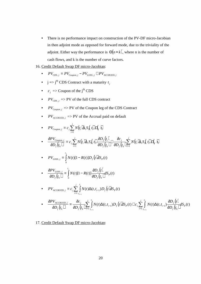
16. Credit Default Swap DF micro-Jacobian:
• jACCRUEDjLOSSjCouponjCDS PVPVPVPV ,,,, +−=
• j => jth CDS Contract with a maturity jt
• jc => Coupon of the jth CDS
• jCDSPV , => PV of the full CDS contract
• jCouponPV , => PV of the Coupon leg of the CDS Contract
• jACCRUEDPV , => PV of the Accrual paid on default
• ( ) ( ) ( )ifi
j
iPiijjCoupon tDtStNcPV ∑
=
∆=1
,
• ( ) ( ) ( ) ( )( ) ( ) ( ) ( ) ( )ifi
j
iPii
kf
j
kf
ifi
j
iPiij
kf
jCoupon tDtStNtD
c
tD
tDtStNc
tD
PV∑∑
==
∆∂
∂+
∂∂
∆=∂
∂
11
,
• ( )∫ −=jt
PfjLOSS tdStDtRtNPV0
, )()](1)[(
• ( )( )( )∫ ∂
∂−=
∂∂ jt
Pkf
f
kf
jLOSS tdStD
tDtRtN
tD
PV
0
, )()](1)[(
• ( )∑ ∫=
−
−
∆=j
i
t
t
PfijjACCRUED
i
i
tdStDtttNcPV1
1,
1
)(),()(
• ( ) ( ) ( ) ( )( )∑ ∫∑ ∫
=−
=−
−−∂∂
∆+∆∂
∂=
∂∂ j
i
t
t
Pkf
fij
j
i
t
t
Pfikf
j
kf
jACCRUEDi
i
i
i
tdStD
tDtttNctdStDtttN
tD
c
tD
PV
11
11
,
11
)(),()()(),()(
17. Credit Default Swap DF micro-Jacobian:

21
• ( ) ( ) ( ) ( ) ( )( ) ( ) ( ) ( ) [ ] ( )∑ ∫
=−−
−−∆+
∂∂
∆=∂∂
−
j
i
t
t
ijkf
ifiiiij
Kf
jCDSi
i
tdPtRttctNtD
tDtStttNc
tD
PV
111
,
1
1,,
• There is no performance impact on construction of the PV-DF micro-Jacobian
in then adjoint mode as opposed for forward mode, due to the triviality of the
adjoint. Either way the performance is ( )kn×Θ , where n is the number of
cash flows, and k is the number of curve factors.

22
Spanning Spline
Formulation and Set up
1. Spline vs. Boot Span: For the purposes of this discussion, the main difference
between spline and boot span is that, in boot span, the segment boundaries HAVE to
line up with the instrument maturity edges. In spline spans, however, additional
criterion-based knots may be used to determine the boundaries (e.g., parametric knot
insertion in line with regression spline approaches).
2. Basic Setup: All instruments and quotes fall into one set of constraints as
( ) l
b
jjlfjl QtDc =∑
−
=
1
0
, where al ,...,1= .
• In general, ba < , so you have ab − degrees of freedom.
3. Local Ordinate Re-formulation: The spline extends from 1−→ bSTART tt . Setting
STARTb
STARTii tt
ttx
−−=
−1
, ( ) ( )∑∑−
=
−
=
⇒1
0
1
0
b
jjlfjl
b
jjlfjl xDctDc . Further, ( ) ( ) 10 === xDtD fSTARTf .
4. Basis Formulation: Setting ( ) ( )∑−
=
=1
0
n
iiif xfxD α ,
( ) ( ) l
b
jjijl
n
iil
b
j
n
ijiijl QtfcQtfc =
⇒=⇒ ∑∑∑ ∑
−
=
−
=
−
=
−
=
1
0
1
0
1
0
1
0
αα . Thus, if an = , there now are a
equations and a unknowns.
5. Monotonicity Preservation in Spanning Splines: The heterogeneity of the calibration
instruments demands special techniques for monotonicity maintenance (Hagan West
(2006) described in detail earlier was a sample).
• Stringent monotonic constraints introduced by Hyman (1983) was relaxed by
Dougherty, Edelman, and Hyman (1989), and this was works well in practice in
its ability to maintain monotonicity (Ametrano and Bianchetti (2009), Le Floc’h
(2013), also implemented in Quantlib (2009)).

23
• Intermediate filter constraints introduced by Steffen (1990) and their variants
treated in some detail by Huynh (1993) – all suffer from the same unnatural
“dip”s or cook bumps.
6. Pros: As always, the degrees of freedom may be expanded beyond a to allow for
optimizing spline construction (covered in the spline builder section).
7. Cons: With many basis functions (esp. for polynomials), the inevitable Runge’s
phenomenon takes over.
Challenges with the Spanning Spline Approach
1. Problems with Cubic Polynomial Spline: Too well known to documented – spurious
inflection, too much concavity/convexity at widely separated predictor nodes (esp. in
long end), and no guarantee of positivity where desired.
• As noted in Le Floc’h (2013), monotone variants (including Hagan and West
(2006), Wolberg and Alfy (1999), Hyman (1983)) of the standard cubic spline
have differing degrees of problems since they are attempt to model the entire span
with a single representation.
2. Problems with Quartic Spline: While this makes the interpolation very smooth
(Adams and van Deventer (1994), van Deventer and Inai (1997), Adams (2001), Lim
and Xiao (2002), Quant Financial Research (2003)), the stiffness needed for shape-
preservation is completely lost. Other troubles as with cubic splines (spurious
inflection, too much concavity/convexity at widely separated predictor nodes (esp. in
long end), and no guarantee of positivity where desired) as well Runge’s swings are
also present.

24
Monotone Decreasing Splines
Motivation
1. These are spline basis functions that monotonically decrease over the given interval.
Valuable for representing discount factors.
2. Why represent discount factors? Because the pay-offs are linearizable in them, so
working with them implies working with the linear rates space representation, and all
the advantages that come with that.
Exponential Rational Basis Spline
1. Basis Function Set:
++
−−
t
ee
t
tt
1,,
1
1,1
2. Monotone Decreasing Nature: Each of the above basis functions is decreasing. For
the functional form to be monotonically decreasing, conservatively speaking, this
imposes the demand that 0=iβ for every i .
• Alternatively, we may also require that no infection exist within the given
segment, but that is hard to enforce.
Exponential Mixture Basis Set
1. Motivation: Since the discounting function goes as te− , an exponential mixture basis
such as tie λ− may be a good choice, as they are both intuitively monotone, and linear
combinations of them produce convexity/concavity.
2. Basis Function Set: tie λ− for 1,...,0 −∈ ni .

25
• Choosing iλ : Since for 2C continuity we require 4 basis functions, we choose
0=Floorλ , Lowλ , Mediumλ , and Highλ . 0=Floorλ accounts for adjusting jumps.
• Typical values can be: 0=Floorλ , %1=Lowλ , %5=Mediumλ , and %25=Highλ .
• Parallel with Tension Splines => iλ are comparable to tension splines.
• With this choice, kC may be maintained for 2≥k , thereby making the forwards
continuous, preserving locality, imparting segment convexity/concavity. Thus all
the smoothing schemes may be maintained.
3. Similarity with exponential/hyperbolic tension splines: Very similar in formulation.
However, given that with exponential/hyperbolic basis set spline at one of basis
functions has a non-negative exponential argument, that basis function becomes
monotonically increasing.
• Further, while estimation of the exponential tension needs to be done extraneously
(Renka (1987)), here we appeal to the intuitive physics, as shown.
26
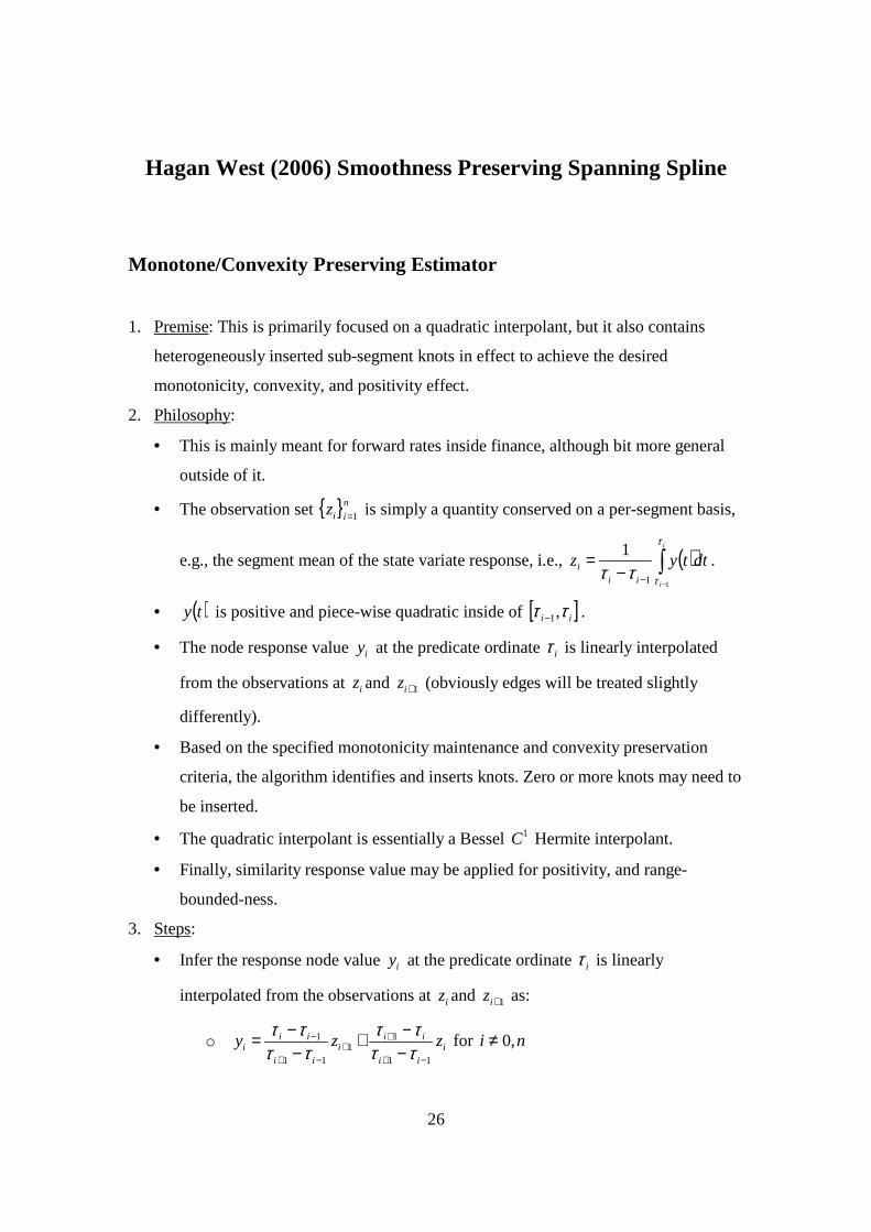
Hagan West (2006) Smoothness Preserving Spanning Spline
Monotone/Convexity Preserving Estimator
1. Premise: This is primarily focused on a quadratic interpolant, but it also contains
heterogeneously inserted sub-segment knots in effect to achieve the desired
monotonicity, convexity, and positivity effect.
2. Philosophy:
• This is mainly meant for forward rates inside finance, although bit more general
outside of it.
• The observation set n
iiz 1= is simply a quantity conserved on a per-segment basis,
e.g., the segment mean of the state variate response, i.e., ( )∫−−−
=i
i
dttyzii
i
τ
τττ11
1.
• ( )ty is positive and piece-wise quadratic inside of [ ]ii ττ ,1− .
• The node response value iy at the predicate ordinate iτ is linearly interpolated
from the observations at iz and 1+iz (obviously edges will be treated slightly
differently).
• Based on the specified monotonicity maintenance and convexity preservation
criteria, the algorithm identifies and inserts knots. Zero or more knots may need to
be inserted.
• The quadratic interpolant is essentially a Bessel 1C Hermite interpolant.
• Finally, similarity response value may be applied for positivity, and range-
bounded-ness.
3. Steps:
• Infer the response node value iy at the predicate ordinate iτ is linearly
interpolated from the observations at iz and 1+iz as:
o iii
iii
ii
iii zzy
11
11
11
1
−+
++
−+
−
−−+
−−=
ττττ
ττττ
for ni ,0≠

27
o [ ]1110 21
zyzy −−=
o [ ]nnnn zyzy −−= −121
• Work out the “Z-score” metric within [ ]ii ττ ,1− :
o ( ) iiiii zyzyg −=−= −−− 111 τ
o ( ) iiiii zyzyg −=−= τ
o Further, we work in the local predictor ordinate space x , where
1
1
−
−
−−=
ii
ixττττ
.
• Apply the appropriate adjustments for the monotonicity/convexity enforcement at
the appropriate zones:
o Case 01 >−ig , 11 221
−− −≥≥− iii ggg [OR] 01 <−ig , 11 221
−− −≤≤− iii ggg :
Here, the function ( ) ( ) ( )221 32341 xxgxxgg ii +−++−= −τ can be used
unchanged, as the original construct is already monotone and convex.
o Case 01 >−ig , 12 −−≥ ii gg [OR] 01 <−ig , 12 −−≤ ii gg : Here, insert a knot
at 1
12
−
−
−+=
ii
ii
gg
ggη . The segment univariate now becomes: ( ) 1−= igg τ for
η≤≤ x0 , and ( ) ( )2
11 1
−−−+= −− η
ητ xgggg iii for 1≤< xη .
o Case 01 >−ig , 121
0 −−>> ii gg [OR] 01 <−ig , 121
0 −−<< ii gg : Here,
insert a knot at 1
13
−
−
−=
ii
i
gg
gη . The segment univariate now becomes:
( ) ( )2
11
−−+= −− ηητ x
gggg iii for η<≤ x0 , and ( ) igg =τ for
1≤≤ xη .

28
o Case 01 ≥−ig , 0≥ig [OR] 01 ≤−ig , 0≤ig : Here, insert a knot at
1−+=
ii
i
gg
gη . Setting 1
1
−
−
+−=Α
ii
ii
gg
gg, the segment univariate now
becomes: ( ) ( )2
1
−Α−+Α= − ηητ x
gg i for η<≤ x0 , and
( ) ( )2
1
−−Α−+Α=
ηητ x
gg i for 1≤≤ xη .
Positivity Preserving Estimator
1. Positivity of the interpolant: Hagan and West (2006) guarantee this by setting he
following bounds:
• [ ]100 2,,0 zyboundy =
• [ ]nnn zyboundy 2,,0=
• ( )[ ]1,min*2,,0 += iiii zzyboundy for ni ,0≠
Ameliorating Estimator
1. Amelioration (i.e., Smoothing) of the Interpolant - Steps:
• #1: Expand the Range at the edges => Add an interval at the beginning and at the
end.
o ( )0101 ττττ −−=− and ( )1202
0110 zzzz −
−−−=
ττττ
o ( )11 −+ −+= nnnn ττττ and ( )12
11 −
−
−+ −
−−+= nn
nn
nnnn zzzz
ττττ
o Complete the linear interpolation of the response variate across all the
intervals as before.

29
• #2: Set the Extraneous Bounds Parametrically/Empirically => Assume that the
left and the right mini-max bounds are set extraneously for each segment, i.e.,
LeftMiniy , , LeftMaxiy , , RightMiniy , , and RightMaxiy , are extraneously set. They may be set
either point-by-point, or using another parametrization. This ensures locality, at
expense of kC , however.
o Check if the given response value is inside of the specified range, i.e.,
( ) ( )RightMiniLeftMiniiRightMaxiLeftMaxi yyyyy ,,,, ,max,min ≥≥ , set as follows:
• If ( )RightMaxiLeftMaxii yyy ,, ,min< , ( )RightMaxiLeftMaxii yyy ,, ,min= .
• If ( )RightMiniLeftMinii yyy ,, ,max> , ( )RightMiniLeftMinii yyy ,, ,max= .
o Otherwise:
• If ( )RightMaxiLeftMaxii yyy ,, ,min< , ( )RightMaxiLeftMaxii yyy ,, ,min= .
• If ( )RightMiniLeftMinii yyy ,, ,max> , ( )RightMiniLeftMinii yyy ,, ,max= .
• #3: Re-work the edges =>
o If 0100 21
zyzy −>− , then 0110 21
zyzy −−= .
o If nnnn zyzy −>− −121
, then nnnn zyzy −+= −121
.
o If 0y is already explicitly specified (as the zero-day rate in some markets)
use that instead.
o Finally, if needed re-apply the positivity enforcement across all the
segments as before.
Harmonic Spline Extension to the Framework above
1. Harmonic Splines and Continuous Limiters extension: Le Floc’h (2013) applies the
harmonic splines originally introduced by Fritsch and Butland (1984), and extends the
monotonicity preserving limiters of Van Leer (1974) and Huynh (1993) by using
rational functions.

30
2. Harmonic Forwards in Hagan-West: Couple of interesting items to note: Given
ii
iii tt
yym
−−=
+
++
1
11 , on substituting iii tzy −= , you get ii mz −=+1 , and ii fs +−=− .
3. Estimation of the node forwards using Harmonic mean: Apply the above now to get
( )( )
( )( ) 111
11
11
11 13
213
21
+−+
−+
−+
+−
−−+−+
−−+−=
iii
iiii
iii
iiii
i ztt
tttt
ztt
tttt
f if 01 >+ii zz , and 0=if
otherwise. After this, the regular Hagan-West may be applied without the need to
enforce monotonic or convexity constraints, as it now is monotonic/convex by
construction.
Minimal Quadratic Estimator
1. Design Philosophy: The algorithm extracts the spline coefficients keeping in mind the
following:
• Formulate using a 2nd degree quadratic polynomial for each segment
• Maintain the Conserved Quantities
• Maintain the Segment Edge Continuities
• Optimize for the linear combination of two penalties:
o Jump of the inter-segment discontinuities on the first derivatives
o Curvature of the second derivative
2. Step #1: Preservation of the Conserved Quantity Set: This results in the following
equation: 2
31
21
iiiiii hchbaz ++=
3. Step #2: Edge Continuity Constraint: 21 iiiiii hchbaa ++=+ .
4. Step #3: Minimize the Penalty:
• Jump of the inter-segment discontinuities on the first derivatives
[ ] ( )[ ] ( ) ( ) 221
21
21
211 4422 iiiiiiiiiiiiiiiii hcbbhcbbhcbbbhcbJ +−+−=+−=−+= ++++
• Curvature of the second derivative [ ] 2222 42 iiiii hcchJ =•=

31
• Complete Penalty Formulation =>
( ) ( ) [ ] ( )1222
22 4421 +−+=•=−+= iiiiiiiiii bbhchcchJJP ωωωω
• ( ) ( ) ( )080480 2
12 >=
∂∂
⇒=−+⇒=∂
∂+ i
iiiiiii
i
hc
Pbbhchc
c
P ωωω, so minimum exists.
5. Equation Set and Unknowns Analysis:
• 2
31
21
iiiiii hchbaz ++= => One per segment => )1( −n Equations
• 21 iiiiii hchbaa ++=+ => One per common edge => )2( −n Equations
• ( ) 02 12 =−+ +iiiiii bbhchc ω => One each for all ic up to 2−nc => )2( −n Equations
• Total number of linear equations => 53 −n
• Total number of unknowns => 33 −n
• As always, the final 2 conditions from natural, financial, or the not-a-knot
clamped boundary conditions.

32
Penalizing Closeness of Fit and Curvature Penalty
1. Basic Setup: As described in the companion Spline Library Documentation,
• Gross Penalizer = Fitness Match Penalizer + Curvature Penalizer
• CFqℜ+ℜ=ℜ λ1
• ( )∑−
=
−=ℜ1
0
2q
ppppF YyW
• ∫+
∂∂=ℜ
12
l
l
x
xm
m
C dxx
y
2. Estimation of λ : While the segment spline coefficients are computed by minimizing
ℜ , λ is often extraneously supplied as a tuner that trades the prefect high degree of
fit to the curvature. Tanggaard (1997) suggests using a few methods to estimate λ :
• Using the GCV criterion as demonstrated by Craven and Wahba (1979) and
Wahba (1990).
• From the smoothing spline viewpoint, set the number of basis functions, then
search for the corresponding λ using the technique listed in Tanggaard (1997).
3. Measurement Filtering vs. Best Fit Weighted Response: These approaches are very
similar, in that the Best Fit Weighted Response “steers” the calibrated spline basis
and their coefficients to accommodate the measurements in the uncertain sense
(potentially by incorporating measurement uncertainty).
a. If the measurement uncertainty/variance is explicitly known, the Andersen
(2005), the Tanggaard (1997), and/or the GCV techniques may be used to
extract better estimate for λ - through Andersen RMS 2γ estimator,
Craven/Wahba’s GCV, or Tanggaard’s trace-based λ estimator.
b. Differences => However, it needs to be remembered that, for current curve
construction methodologies, a key requirement is the 2γ matches (i.e., exactly

33
reproducing state estimations) – which is not the typical case for the filtered
state estimations.
4. Effectiveness of State Representation Quantification Metric: The combination of
curvature penalty, the length penalty, and the closeness of fit penalty must be taken
together to gauge the effectiveness of the chosen Quantification Metric/Smoothing
spline scheme set. Alternatively, full simulations of the manifest metric (with induced
noise terms as explained in for e.g., Fisher, Nychka, and Zervos (1994)) and their
corresponding evaluations are also appropriate, although they tend to be time
consuming (and possibly overkill).

34
Extrapolation in Curve Construction
1. Latent State Choice for the Extrapolator: The quantification metric used to
extrapolate the latent state may be completely different from that used to infer
within the span.
• This clearly indicates that the span spans the extrapolated range as well.
Further, the extrapolator should be a property of the Span, not any stretch.
2. Extrapolator Construction: At the span edges, the kC continuity constraints may
be passed onto the extrapolator as well. These may take the form of the stretch
boundary conditions (natural/financial etc).
3. State Space Extrapolation using Synthetic Observations: This is really what it is.
In particular, to get the desired left/right boundary behavior, you may insert
synthetic observations at either end to produce the desired custom behavior (this
may also be used in lieu of the explicit boundary condition specification).

35
Multi-Pass Curve Construction
Motivation
1. Introduction: This is composed of one shape preserving pass on the inferable state
quantification metric, followed by on or more “smoothing passes”.
2. Shape Preserving Pass: The shape preservation pass occurs on the “native designate”
measure, preferably one that is linearly inferred from the manifest measure. The
primary objective of the shape preservation pass is to maintain the monotonicity, the
convexity, the locality, and possibly the positivity of the quantification metric.
• The output of the shape-preserving pass is a span on the quantification metric that
is “well-behaved”, and one that contains a new set of “truthness” nodes on which
the eventual smoothing can be done.
3. Shape Preservation Variants:
• Linear in the discount Factor Quantification Metric => They are obviously the
best shape preserver (owing to the perfection in the match and zero curvature
penalty), but they no inherent convexity/concavity in them, so it gets harder fort
the smoothing stage.
• Constant forward rate bootstrapping may also be used.
4. Smoothing Pass: Here you smooth on the appropriate quantification metric that is
deemed to be a better hidden-state characterizer.
5. Advantages of the Shape-Preserving Pass:
• Separation between Shape-preservation and smoothing.
• Choice of convenient, yet potentially different metrics across shape-preserving
and smoothing.
• The final state representation quantification metric need not be linear on the
manifest measure.

36
• The granularity/precision of fit of the curve automatically adjusts with
information (i.e., cash flow event dates such as pay dates), thereby making it
inherently more precise.
• PCHIP techniques may be applied more conveniently on the smoothing pass.
• Other closeness of fit techniques (such as least squares methodologies, etc: )
become much more relevant on the smoothing pass.
6. Disadvantages of the Shape-Preserving Pass:
• Calculation overhead penalty associated with the dual pass (although, by choosing
linearity between manifest measure/quantification metric and the quantification
metric/ quantification metric combinations this adverse impact maybe reduced).
• Artifacts produced during shape-preservation (again, there will be artifacts
associated with just about any basis representation).
Bear Sterns Multi-Pass Curve Building Techniques
1. DENSE Methodology: This method is outlined in Nahum (2004).
• Cash/Forwards => Piece-wise constant forwards. Turn Spreads imposed as
needed.
• Swaps => Shape Preserving uniform tension splines.
• RAW Swaps Inputs => Quarterly swap rates are now re-implied from the curve
constructed in the earlier stage.
• From these new swap quotes, a new curve is constructed using quarterly constant
forward rates (constant forward rates methodology is called RAW).
2. DUAL DENSE Methodology: Again, this method is outlined in Nahum (2004).
• Short end (Cash/Futures) => Daily forwards (i.e., constant daily forwards or cdf)
latent state implied.
• Long End => Same methodology as DENSE, except for the non-uniform tension
that is applied across quarterly swap contracts.

37
Transition Spline (Or Stitching Spline)
Motivation
1. Spline per Instrument Grouping: Another possibility is to use transition spline to
bridge across different instrument groups – this simply needs to adjust to the
smoothness/truthness constraints of each of the instrument groups.
• Essentially, transition splines connect spline families across instrument group
(each instrument essentially belongs to its own spline cluster).
2. Design:
• May use discontinuous Hermite splines in the transition area, or higher order basis
(say, with an appropriate kC constraint), or even an optimizing transition spline.
• Instrument choice is critical if we are to avoid steep transition slopes (esp. tight
group gaps, and steep measure drops). These are challenges in any mechanism,
but possibly a lot more here.
• Construct single instrument spanning spline curves, then demarcate/spec out the
instrument range, finally bridge in the transition splines.
• Transition splines may also be used to stitch in arbitrary instruments together,
each belonging to its own separate group, although it is hard to find a practical
need for such a construct.
• In general, instrument group boundaries need not strictly coincide with the
instrument termination nodes (esp. in case of stitch-in splines). Boundaries may
be inserted using any of the appropriate knot insertion techniques.
3. Advantages:
• These preserve the curve character embedded in each instrument grouping, which
can be a sub-set of a vaster instrument set.
• By retaining the localization to the corresponding instrument grouping, the hedges
produces by the transition spline may, in principle, be better than those produced
by the typical ones.

38
4. Disadvantages:
• Of course, by construction, they do not allow for overlapping instrument groups
(which, however, may not be a problem in the practical world). This forces a
decision on the instrument set choices and boundaries.
• Technically, the single “natural spline boundary condition” is not applicable
across all the unprocessed instrument groups – this is really what is compromised.
o How much the effectiveness is compromised due to the above may be
estimated using targeted metrics, say the span DPE.
5. Transition Segment in the Transition Spline: This needs at least 22 +k basis
functions for representation, as it needs to “mate out” the left stretch and the right
stretch ( kk + for each of the kC continuity spec - plus 2 more, one at each end to
match up the point node).
6. Using Transition Splines for Calibration Instrument Selection: As shown in Figures 2
and 3 below, the transition stretch represented in figure 2 is narrower, and therefore
more abrupt/jumpy (with corresponding implications for the forward rates) than that
in Figure 3. A criteria based approach is necessary to develop this.
Stretch Modeling Using Transition Splines
1. Information Propagation across Stretches: All the truthness/smoothness information
of the predecessor stretch is captured by the stretch’s calibrated span parameters. Any
state inference for predictors in a given domain needs to be deferred to the domain’s
span stretch.
• The corollary to the above is that trailing stretches will typically need information
from the leading stretches for state inference/estimation (leading/trailing here are
set in regards to the inference flow (or information flow)). Applied to discount
curve cooking, the leading stretch that uses cash instruments is essentially self-
calibrating, whereas the trailing stretch of swap instruments is going to rely on
information that comes out of the cash calibration. Going into swap segments, the

39
information will propagated in the form of RVC’s, so they will need to be handled
right from the left-most segment of each stretch.
• Regular Stretches vs. Finance Curve Stretches => For typical stretch construction,
all you need is the transmission of the segment-to-segment continuity constraints
through kC . For segment curve builders, however,
( ) ( )10,...,int −= Ni SegmentSegmentfSegmentConstra , i.e., more construction
information in addition to just the kC is required (mostly via explicit evaluation
of arbitrary points in earlier segments’ stretches).
2. Response Stretches: Markov response state variables may follow distinct behavior in
different predictor stretches. For example, the discount factor/zero rate/swap rate may
be characterized using one set of representations for the cash stretch, whereas the
swap stretch may use a different set.
3. Why Response Stretches exist: Is it simply because of the instrument choice (cash for
the front end, swap for the back end, etc:), or is there a more fundamental driver?
Can’t say one way or the other, but the fact is we empirically attempt to match point-
by-point in a left to right manner (we do this today) without compromising the
empirical characteristics of each instrument group. We call each of these groups
manifest groups, since they could be result of specific product manifest measures).
4. Manifest Group Contribution to the Response Signal Strength: Say that a signal
strength contribution to a specific response signal is proportional to its liquidity (to
improve accuracy, you may make it sided liquidity). As you move from left to right in
the predictor space, by working it in terms of the liquidity-fade of the left stretch to
the liquidity-explode of the right stretch, you may be able to characterize the response
space more naturally (with less dependence on explicit stitching splines, or on
artificially inserted knots).
5. Liquidity-Fade and Liquidity-Explosion in practice: In practice the actual predictor
ordinates across the manifest stretches will be too discrete for tracking the liquidity-
fade and liquidity-explosion. Thus, it may be more appropriate to operate on predictor
windows. If convenient and admissible, the predictor window boundaries may also
coincide with the segment boundaries.

40
Stretch Partition/Isolation in Transition Splines
1. Definition: A given calibratable predictor ordinate/response realization space is called
a span. The span is partitioned into stretches. Stretches can be either core stretches or
transition stretches. Both the core stretches and the transition stretches are built from
segments (within which the response values may be represented using basis splines).
Core stretch are inferred to truthness and the smoothness signals, and the transition
stretches provide the explicit bridge between the core stretches that may not be
possible using the plain core stretch representations.
2. Information Patterns: With a higher unit, information propagation is associated with
each sub-unit entities below. Across peer units, information exchange is materially
similar in nature. Across higher units, information exchange may be more
parsimonious (although it may still happen between lower entities belonging to the
higher units).
3. Information Localization and Transmission: Intra-segment information propagation
occurs through smoothness constraints such as kC .
4. Stretch-Level Information Localization: In the spline case, this happens though
boundary-condition delimitation/isolation (i.e., natural/financial/clamped boundary
conditions based isolation is applicable to within a single stretch).
5. Stretch-Stretch Transmission: These are not bound by the equivalent isolation
constraints, therefore the connecting/transition splines need to have a qualitatively
different nature.
6. Transition/Connecting Splines: By definition, since they are the bridge between the
stretches, they need to have greater degrees of freedom for a complete bridge.
Knot Insertion vs. Transition Splines

41
1. Equivalence: In some sense, they are equivalent in that inserting knots also attempts
to complete the bridge. However, transition splines are more customizable, since the
splines that flank the knots are assumed in the literature to be variants of the others.
2. Advantages on Knot Insertion: Remember that transition splines need 22 +k basis
function. Thus, for high k , you are stuck with higher-order polynomials (for e.g.),
along with all the Runge’s oscillations/instabilities that it brings. Suitable choice of
knots may minimize this.
3. Advantage of Transition Spline: Knots are stretch response altering (via their kC
criteria), whereas transition splines enable each stretch to retain their character.
Overlapping Stretches
1. Premise: By definition, stretch fade-out and stretch explode axiomatizations imply
predictor ordinate overlapping stretches.
2. Stretch Boundaries: Each stretch constituting an overlapping stretch needs to have its
boundaries identified. What do not necessarily overlap are the smoothness
constraints.
3. Overlapping Stretch – Problem Statement:
• Predictor Ordinate Stretches overlap.
• Stretches (and by implication, their predicate ranges) are contained/telescoped.
• Smoothness constraints may not overlap, in which case they are posited to be
distinct in each of the constituent stretches.
• Truthness should be strictly telescopically contained/localized, i.e., there is a
manifest measurement exclusivity to each stretch.
• A consequence of this is that the inferred state response variable will be
propagated, but not (necessarily) the smoothness criterion.

42
Index/Tenor Basis Swaps
Component Layout and Motivation
1. Basis Swap Market: Although Basis Swaps did exist even earlier (Tuck man and
Porfirio (2003), Morini (2008)), post-crisis segmentation (attributable, among other
things, to the preference towards receiving higher frequency payments) intensified
these differentials (Mercurio (2009)).
2. Origins of Basis Swap Existence: In principle, these are expected to represent
embedded duration counter-party credit risk. The “good” model should couple
embedded credit risk with the sided flow dynamics (i.e., the credit quality of the
counter-party that enters into the long/short side of the greater frequency leg, etc :)
3. The Discounting Curve: Challenges regarding the uniqueness in relation to the
instrument choice for building the discount curve have been identified by Henrard
(2007). The issues stem primarily from the uncollateralized nature of deposits and
forwards, therefore, these are typically replaced by OIS/EONIA and Futures
(Madigan (2008)).
• Interest Rate Swap continues to be used for the discount curve calibration, as it
possesses the following characteristics:
o Par IRS’es are collateralized at inception.
o Collateral margining may be applied over time.
o IRS is the only liquidly available fix-float swap, and as such effectively
implies just a single forward curve.
• Convexity adjustment for extracting the rate from future/forward price => Since
futures/forwards act effectively as a zero coupon bond, the transformation of price
to the latent zero/forward rate requires a dynamical volatility based curve
evolution model. Sophisticated, comprehensive approaches are available in
literature (see for e.g., Kirikos and Novak (1997), Jackel and Kawai (2005), Brigo
and Mercurio (2006), Piterbarg and Renedo (2006)); common practitioner

43
approaches, however, employ simpler approaches such as the Hull-White one-
factor short-rate model (Hull and White (1990)).
4. Multi Curve vs. Forward Smoothness: Given that the discount curve and the forward
curve are essentially distinct in the multi-curve latent state, the stringent demands that
all forwards stay smooth (as in the single discount curve that covers all the basis
curve scenarios) may be relaxed.
• Forwards Implied in the Discount Curve => Since the forwards are used only for
the “core” tenor pillars in the discount curve, only those forwards need to be
smooth (e.g., 6M forwards). By discount curve construction this will typically be
the case, as the forwards period will always straddle/span fully a single reset
pillar.
5. Point- vs. Convolved-Measure State Transform:
• Point-Measure transform refers to the one-to-one transform between a state
measure at a predictor ordinate and its corresponding observation (e.g., discount
factor from zero-coupon bond price observations). Since these may be expressed
as straightforward transformations, the observation-state non-linearity may be
easily accommodated.
• Convolved measure-state transforms introduce what are effectively observation
constraints across predictor ordinate/state response combinations. Non-linearity
introduces complications, therefore usage of spline-based linearization constraints
are highly effective.
6. Reset-Date Forward-Rate Pair Constraint in Discount Curve Building: The yM tenor
(e.g., MyM 6⇒ ) may be extracted only at the reset start/end date (depending on the
reset rate-rime axis label) from the discount curve, i.e., only the pair
yMForwardyM , makes sense. In other words, this is the only set of dates for which
the information on forward rates is available. Splining may be an option at the other
dates.
• yM Tenor/DF Relationship => ( ) ( ) ( )∑=
−∆=m
jjfjyMyM tDtFjjPV
1
,1 . For yMPV to
be telescoped away into ( ) ( )jffyM tDtDPV −= 0 , the requirements are: Period

44
Accrual End Date == Period Reset End Date == Period Pay Date. This is the main
reason why the period dates are adjusted before the cash flows are rolled out.
7. Alternative View: Discount Curve IS the yM Forward Curve: To automatically
ensure uniqueness and consistency of the latent state space, it may also be more
restrictively imposed that the nativeyM Forward Curve be implied entirely off of the
discount curve. Thus, the nativeyM Forward Curve may now be implied at all nodes,
not just at the reset nodes as postulated earlier. This automatically eliminates the state
basis between these measures; further, this is still not too restrictive in terms of the
nativeyM Forward Curve smoothness for same reasons as before.
8. Basis between the yM Forward Curve and the Discount Curve: Given that basis
constraints are of paramount consideration in other markets, why not look at the basis
between discount curve and its native forward curve? This is because neither the
latent state underpinning the forward curve or that underpinning the discount curve is
entirely observable (unlike, say basis between a bond and the issuer’s underlying
CDS). Thus an extraneous observation model is necessary. By convention, the current
practice achieves this by construction – the formulation mandates that the discount
curve and the “discounting-native” forward curve be alternate quantification metrics
of the same latent state.
Formulation
1. Float-Float Swap Setup: The phenomenology and flow details laid out in Figure 5 are
based off of descriptions and details provided by ISDA (2000), Ametrano and
Bianchetti (2009), Bianchetti (2009)). The two swap legs are:
• The “known” or the “Reference” leg. Forwards of this leg come from the discount
curve’s IRS contracts, and 6M LIBOR/EURIBOR is the most common such
tenor. We generalize this with a basis spread, i.e., the “effective” forward is
MM SF 66 + , where MF6 and MS6 stand for the corresponding forward and the
spread.

45
• The “unknown” or the “Derived” leg with a tenor of xM . Forwards of this leg are
computed from the corresponding basis market quotes. We generalize this with a
basis spread, i.e., the “effective” forward is xMxM SF + , where xMF and xMS stand
for the corresponding forward and the spread.
2. Basic Formulation Setup:
• ( ) ( )[ ] ( )∑=
+−∆=m
jjfxMjxMxM tDStFjjPV
1
,1
• ( ) ( )[ ] ( )∑=
+−∆=b
aafMaMM tDStFaaPV
1666 ,1
• Equivalence of xMS and MS6 => Since both xMS and MS6 are additive, we work
in a space that is essentially an adjusted forward rate space, with
MMAdjM SFF 66,6 +→ and xMxMAdjxM SFF +→, . While this is straightforward to
accommodate in the case of M6 , from a calibration point-of-view, we work off
of a biased xM space, and re-adjust back after splining.
3. Basis Swap Calibration Formulation: MxM PVPV 6= implies that
( ) ( ) ( ) ( ) ( ) ( ) ( ) ( ) ( )∑∑∑==>
−∆−−∆=−∆l
l
m
jjfjAdjxM
b
aafaAdjM
m
mjjfjAdjxM tDtFjjtDtFaatDtFjj
1,
1,6, ,1,1,1
. For all but the left most basis swap, 0>lm .
4. Basis Swap Calibration Constraint Specification:
• Set ( ) ( ) ( ) ( ) ( ) ( )∑∑==
−∆−−∆=ℵlm
jjfjAdjxM
b
aafaAdjMm tDtFjjtDtFaa
1,
1,6 ,1,1 . Notice that
mℵ maybe fully computed from before.
• Recognize that ( ) ( )∑=
=n
iiiAdjxM tftF
1, β .
• Combine above to get the calibration constraint
( ) ( ) ( )∑ ∑= >
−∆=ℵn
i
m
mjjfjiim
l
tDtfjj1
,1β .
5. Reference/Derived Par Spread Relations: For parity,
DerivedDerivedDerivedferenceferenceference SDVPVSDVPV 0101 ReReRe +++ . Setting 0=DerivedS ,

46
ferecne
Derivedferecneferecne DV
PVPVS
Re
ReRe 01
+−= . Likewise,
Derived
DerivedferecneDerived DV
PVPVS
01Re +
−= .
Remember that both ferecneSRe and DerivedS can be negative.

47
Multi-Stretch Merged Curve Construction
Motivation
1. Discount Curve composed of Forward Rate Stretches: The discount curve span may
be viewed as being composed of overlapping/non-overlapping forward rate stretches,
i.e., adjacent or otherwise 3M Tenor forward stretch, 6M Tenor forward stretch, etc:
This visualization is a consequence of the representation of the “single discount curve
latent state”, whose alternate/parallel quantification metrics are composed off of these
stretches of forward rates that share the latent state space with the global discount
curve.
2. Out-of-Native Stretch Arbitrage: If one seeks a forward rate outside these stretches
for the given tenor/index combination, there can be no expectations of no-arbitrage,
i.e., there will be a basis between the forward implied by this latent space
quantification metric and the forward rate under consideration.
• Likewise, if inside the stretch, there should be no implied basis, since the diver
latent state is identical/fully correlated.
3. Merging/de-merging of the Latent State along the Predictor Ordinates: If you imagine
the rates state space being characterized by a set of latent states (which may be highly
correlated), each state may ideally be characterized by a quantification metric that is
native to the state physical view. Thus, the unification of the sub-states in a stretch
may be viewed as state-merging (i.e., one quantification metric may be inferred from
another within a merged space via a trivial transformation).
4. Probit-based Latent State Merger Analysis: Given that the discount/forward latent
states merge/de-merge, it might it particularly amenable to a common-factor probit
(or even a logistic) analysis of the merger driver dynamics. The challenge would then
be to link the driver dynamics to the maturity based predictor ordinate.

48
Merge Stretch Calibration
1. Cross-Stretch Calibration: Clearly the latent state span characterized by multiple
stretches will in turn be composed of latent state merge sub-stretches. The merged
stretch may be followed by de-merged stretch, etc:
2. Calibration Challenges:
• What would be most optimal cross-representation inside the merge sub-stretch
(i.e., the state representation needs to be smooth for both the discount factor latent
state as well as the forward curve latent state)?
• On the other hand in the solitary segment sub-stretch, you may have more
representation freedom, but may still need to carry over the smoothness
constraints from the merged sub-stretch. How can this be done? Can the transition
spline treatment above be effectively employed here? In other words, what would
be appropriate transition zone applicable to the sub-stretch?

49
Spline-Based Credit Curve Calibration
1. Overview: Andersen (2003) has made an initial effort in this regard.

50
Inference-Based Curve Construction
Curve Smoothing in Finance
1. Unconstrained Curve Smoothing:
• Applicable primarily for rates/semi-liquid FX curves. Smoothing can be done
here without constraints.
• Smoothing may also be applicable to the quotes for a given instrument across
several days.
• Smoothing may also be applied over a single day curve – particularly to model the
switch over from instrument to instrument (e.g., between EDF and Swaps).
2. Constrained Curve Smoothing: Applicable, for e.g., to the case of a hazard curve. The
smoothing basis functions/weights combination must guarantee, from a formulation
PoV, that the implied hazard rate is always greater than zero.
3. Liquidity Based Weighted Signal Smoothing:
• Fidelity at the “liquid bonds” / benchmark bond nodes
• Lower fidelity penalty, but higher smoothness penalty for the less liquid bonds
• Penalty measure is calculated off of the relative liquidity ranking measure (for
e.g., TRACE)
4. Non Bayesian Liquidity Based Smoothing:
• Liquidity indicator serves as a roughness/fidelity magnifier/dampener
• Also need to penalize for over-parameterized fits using AIC/BIC (also CV/GCV –
given that this is essentially a frequentist case).
• These can be applied not just for bonds, but also CDS, rates, FX – even less liquid
ones.
5. Bayesian Extension to the above: Any parametrically specified distribution needs to
evolve using a hyper-prior, and the Wahba parametric Bayesian priors need evolving
too.

51
6. Nodal Jacobian/Sensitivity Impact: As always study the impact on the locality of the
perturbation, as well as the ease of Jacobian estimation – esp. if the calibration needs
to occur through MCMC, non-linear optimization etc:
7. Mixtures of splines and smoothness penalties: As always estimate the impact on
monotonicity, convexity, shape preservation etc: - the category item checks in
Goodman’s paper.
8. Knot Selection Tips: Need some tips in both situations – frequentist and Bayesian.
9. Suggestion on the locally adaptive Parametric Form: Examine the knot-to-knot
smoothness and penalty by using additional locally adaptive microstructure
parameters and their implications.
10. Goodman and Eilers/Marx Talking Point Issues: Criterion check for these specific
“goodness” checks.
Bayesian Curve Calibration
1. Bayesian based past knowledge incorporation of survival probabilities: Given that the
prior’s, the posterior’s and the likelihood’s are all probabilities, perhaps the best
starting point is for applying it to the problem of updating the survival probabilities
and recovery rates based on price observations.
2. Curve Updating techniques: Need grand new formulation techniques that are based
on AD and Bayesian methodologies as part of the curve updating strategies based
upon individual incoming observations and their strength signals.
3. Curve Construction off of hard/soft signals: Hard Signals are typically the truthness
signals. Typically reduce to one calibration parameter per hard observation, and they
include the following:
• Actual observations => Weight independent true truthness signals
• Weights => Potentially indicative of the truthness hard signal strength
Soft signals are essentially signals extracted from inference schemes. Again, typically
reduce to one calibration parameter per soft inference unit, and they include the
following:

52
• Smoothness signals => Continuity, first, second, and higher-order derivatives
match – one parameter per match.
• Bayesian update metrics => Inferred using Bayesian methodologies such as
maximum likelihood estimates, variance minimization, and error minimization
techniques.
4. No-arbitrage hard signals: Simply indicates that the given hard observation is out of
bounds and irreconcilable (i.e., no solution can be found) within the axiomatic
inference space dictated by:
i. The parameter sequence implied by the other set of hard signals.
ii. The model axiom schemes.
iii. The inference rules.
• Directionality “bias” is inherent in calibration (e.g., left to right, ordered sequence
set, etc:) – this simplifies the problem space significantly. Therefore, the same
directional bias also exists in the calibration nodal sequence.
5. Parameter Space Explosion: Generally not a problem as long as it is segment-
localized (in matrix parlance, as long the transition matrix is tri-diagonal, or close to
it), i.e., local information discovery does not affect far away nodes/segments.
• Also maybe able to use optimization techniques to trim them.
6. Live Calibrated Parameter Updating: Use automatic differentiation to:
• Estimate parametric Jacobians (or sub-coefficient micro-Jacobians) to the
observed product measures.
• Re-adjust the shifts using the hard-signal strength.
• Update the parameters from the calculated shifts.
• Re-construct the curve ever so periodically (for a full re-build, as opposed to the
incrementals).
• Remember that AD based parametric updates break smoothness (including
continuity as Bayesian MLE’s) – so use a tolerance in the shift if this is
acceptable.
7. Causality Bayesian Network DAG For Credit Curve Building: See Figure 1.

53
• DAG searches are not really needed, since here they maybe formulated
conceptually/axiomatically, as opposed to being established through a search
mechanism.
8. Financial First Principles SKU: Following concepts are the core components that can
be used to create the curve construction SKU:
• Time Value of Money.
• Latent Default Indicator.
• Recovery on Default.
• Imbalance premium/discount (for FX, Basis Swaps, etc.)
9. Financial Signal Analysis: Need special analysis techniques to pick out “event trends”
from “concept jumps”, even for highly liquid instruments.
• Liquidity-based Signal Extraction =>
• Identify a liquidity metric
• Imply the “perfect liquidity” – the point at which there is no premium
• Compute the liquidity metric for each security
• Regress (or conceptually determine, or fit) the bid-ask spread to inverse
liquidity (remember that even benchmarks only have finite liquidity, not
infinite) for each security
• Try to slap in a secular “event premium” across all the instruments, over and
above liquidity
10. Systemic Finance Variables Evolution: Given that every measurement is uncertain to
within bounds, it stands to reason that every distribution is also a true distribution (to
within the tolerance provided by the corresponding sufficient statistics, and over a
finite observation window) of the technical state of the world (i.e., technical =
fundamental + a bias).
11. Technical to Fundamental Bias Estimation: This should result from the flow of the
information. Non-technical/Fundamental may possibly be estimated using a bias
correction applied to the technical signal – Bayesian/frequentist techniques may be of
value here.
• Proxy for non-technical behavior => Identify the non-market proxies for the
fundamental drivers, and estimate market drivers as possibly lagging indices.

54
12. Bayesian Decomposition of Technical Signals: In general, the signal core drivers are
limited (like systemic/idiosyncratic factors – alternatively, the latent state
quantification metric), but the product specific manifest measures are more varied.
Bayesian frameworks well suited for these.
13. Financial Stretch Identification: Bayesian classification techniques can be readily
adapted for these purposes – in fact, with abundance of data, these techniques are
very appropriate now.
Sequential Curve Estimation
1. Calibration Framework Drivers: Calibration is considered to occur FOR a hidden
state Sr
, which is quantified using the quantification metric Xr
. Xr
is estimated from
the manifest measure Mr
.
2. Product-Measure Point-of-View: From the Dempster-Shaefer/Kalman Filter/Linear
Quadratic Estimator point-of-view, the Kalman Hr
matrix probabilistically
transforms the hidden state quantification metric to an observation measure, e.g., the
latent forward rate manifests itself through the swap rate.
3. Segment/Span Nomenclature vs. Curve Calibrator Nomenclature: Call the Curve
Calibrator the Dempster-Shaefer Calibrator. Under this:
• LSQM (Latent State Quantification Metric) => Elastic Variate
• State Dimensions (Tenor Axis, X/Y Axis of predictors) => Inelastic Variates
• Thus, the predictors are inelastic, and the responses are elastic.
4. Linearization of LSQM over the predictor axes: The Kalman Hr
observation
transformer should just linearize Mr
onto the space of Xr
over the predictor
dimensions. Non-linearity of Xr
over the predictors is handled through basis splines.
5. Hidden State Evolution vs. Hidden State Representation: The Kalman Hr
matrix is
more of a state modeling and state representation matrix (i.e., the update part that is
fully local to the current time slice) that already brings in the manifest measure
LSQM transformation model.

55
6. The Curve Builder Hr
matrix: Due to the above, the curve builder Hr
matrix needs to
accommodate the 2 possible uncertainties:
• Uncertainty in the manifest measure
• Uncertainty in the manifest measure LSQM transformation model. If this
transformation is non-parametric, then treat it as certain/deterministic. If it is
parametric, then use MLE/MAP to the handle the parameter estimation.
7. UKF Techniques applied to evolve the Curve Builder Hr
matrix: Potential non-
linearity in the curve builder Hr
may be handled using the Jacobian EKF and/or the
sigma-point UKF schemes.
8. The Curve Builder Fr
matrix: The Curve builder Fr
Matrix dictates the evolution
from it to 1+it as ii LSQMFLSQM ×=+
r
1 . This should be explicitly
posited/formulated. Again, use splining to linearize.
9. Financial Noise Covariance Estimation: May be able to extraneously determine these
covariance independent of the state evolution model (if not, we may have to rely on
techniques such as ALS (Rajamani (2007), Rajamani and Rawlings (2009)).

56
Appendix A: Some Trivial Analytical Bond Math Results
1. Price when Yield Equals Coupon: Given the following:
• Annualized Coupon => r
• Payment frequency => f
• Per period yield => y
• Per Period Coupon Payment => f
rc =
• Number of coupon periods to maturity => n
• ( )( ) ( ) ( ) ( )
nn
n
n
mmn
n
mm
dd
dcd
yy
c
yy
frPV +
−−=
++
+=
++
+= ∑∑
== 1
1
1
1
11
1
1
/
11
where
yd
+=
1
1.
• Now, if you are just past a coupon pay (so that clean == dirty), and if 1=PV ,
then we get cyc
ddd
dcd n
n
=⇒+
=⇒+−
−=1
1
1
11 . QED.
2. Par Yield Dirty Price at a non-coupon Date: If ξ is the accrual fraction corresponding
to the accruing period, then ( ) ( ) ( ) ( ) nnDirty
yy
c
y
c
y
cPV +++ +
++
+++
++
= ξξξξξ
1
1
1...
11 1
=> ( ) ( ) ( ) ( ) ( )ξξξ
ξξy
c
yy
c
yy
cPV
n
n
mmDirty +
+=
++
+++
+= ∑
= 1
1
1
1
11
1
1 1
.

57
Appendix B: Per-trade Risk Isolation Components
1. Underlier Security Price Market Risk
2. Discount Factor Risk
3. Forward Rate Risk
4. Currency/FX Risk
5. Basis Risk (on any Risk Factor)
6. Funding Risk
7. Collateral Risk
8. Counter-party Risk

58
References
• Adams, K. and D. van Deventer (1994): Fitting yield curves and forward rates curves
with maximum smoothness, J. Fixed. Income. 4 (1): 52-62.
• Adams, K. (2001): Smooth Interpolation of Zero Curves, Algo Research Quarterly,
March/June, 11 – 22.
• Akima, H. (1970): A New Method of Interpolation and Smooth Curve Fitting based
on Local Procedures, J. Association for Computing Machinery 17 (4): 589-602.
• Ametrano, F., and M. Bianchetti (2009): Bootstrapping the Illiquidity, Modeling
Interest Rates: Advances for Derivatives Pricing.
• Andersen, L. (2003): Reduced Form Models: Curve-Construction and the Pricing of
the Credit Swaps, Credit Derivatives: The Definitive Guide, Risk Books.
• Andersen, L. (2005): Discount Curve Construction with Tension Splines, SSRN
eLibrary.
• Andersen, L., and V. Piterbarg (2010): Interest Rate Modeling – Volume I:
Foundations Vanilla Models, Atlantic Financial Press.
• Barzanti, L., and C. Corradi (1998): A Note on the Interest-Rate Term Structure
Estimation using Tension Splines, Insurance: Mathematics and Economics 22: 139-
143.
• Brigo, D., and F. Mercurio (2006): Interest-Rate Models – Theory and Practice
Springer.
• Rebonato, R. (1998): Interest-Rate Option Models, 2nd Ed., John Wiley & Sons.
• Burden, R., and D. Faires (1997): Numerical Analysis, Brooks/Cole Publishing Co,
New York, NY.
• Chambers, D. R., W. T. Carleton, and D. W. Waldman (1984): A New Structure to
the Estimation of the Term Structure of Interest Rates, Journal of Financial and
Quantitative Analysis. 19: 233-269.

59
• Christensen, J. H. E., F. X. Diebold, and G. D. Rudebush (2007): The Affine
Arbitrage-Free Class of Nelson-Siegel Term Structure Models Working Paper 2007-
20 Federal Reserve Board of San Francisco.
• Coroneo, L., K. Nyholm, and R. Vidova-Koleva (2008): How Arbitrage-Free is the
Nelson-Siegel Model? Working Series Paper 874 European Central Bank.
• Cox, J. C., J. E. Ingersoll, and S. A. Ross (1985): A Theory of the Term Structure of
Interest Rates, Econometrica. 53: 385-407.
• Craven, P., and G. Wahba (1979): Smoothing Noisy Data with Spline Function:
Estimating the correct Degree of Smoothness by the Method of Generalized Cross
Validation, Numerische Mathematik. 31: 377-403.
• De Boor, C. (1978, 2001): A Practical Guide to Splines, Vol. 27 of Applied
Mathematical Sciences, Springer-Verlag, New York.
• De Boor, C. and B. Schwartz (1977): Piecewise Monotone Interpolation, Journal of
Approximation Theory 21: 411-416.
• Delgado, M. A., and P. M. Robinson (1992): Non-parametric and Semi-parametric
Methods for Economics Research, Journal of Economic Surveys 6: 201-249.
• Diament, P. (1993): Semi-empirical Smooth Fit to the Treasury Yield Curve, Journal
of Fixed Income 3: 55-70.
• Dougherty, R., A. Edelman, and J. Hyman (1989): Non-negativity, Monotonicity, and
Convexity Preserving Cubic and Quintic Hermite Interpolation, Mathematics of
Computation 52 (186): 471-494.
• Duchon, J. (1976): Interpolation des Fonctions de deux Variables suivant le Principe
de a Minces, RAIRO Analyse Numerique 10: 5-12.
• Duchon, J. (1977): Splines minimizing Rotation-Invariant Semi-norms in Sobolev
Spaces, Lecture Notes in Mathematics (ZAMP) 57: 85-100.
• Eilers, P. H. C., and B. D. Marx (1996): Flexible Smoothing with B-Splines and
Penalties, Statistical Science 11 (2): 89-121.
• Eubank, R. L. (1988): Spline Smoothing and Non-parametric Regression, Vol. 90 of
Statistics, Textbooks, and Monographs, Marcel-Dekker.
• Fisher, M., D. Nychka, and D. Zervos (1994): Fitting the Term Structure of Interest
Rates with Smoothing Splines.

60
• Fritsch, F., and J. Butland (1980): An Improved Monotone Piecewise Cubic
Interpolation Scheme, Lawrence Livermore National Labarotary Preprint UCRL.
• Fritsch, F., and J. Butland (1984): A Method for constructing Local Monotone Cubic
Piecewise Interpolants, SIAM Journal on Scientific and Statistical Computing 5: 300-
304.
• Fritsch, F. N., and Carlson, R. E. (1980): Monotone piecewise cubic interpolation.
SIAM J. Numer. Anal. 17: 238-246.
• Golub, B., and L. Tilman (2000): No Room for Nostalgia in Fixed Income Risk
Magazine 44-48.
• Hagan, P., and G. West (2006): Interpolation Methods for Curve Construction,
Applied Mathematical Finance 13 (2): 89-129.
• Hagan, P., and G. West (2008): Methods for Curve a Yield Curve, Wilmott Magazine:
70-81.
• Hardle, W. (1990): Applied Non-parametric Regression, Cambridge University
Press.
• Hastie, T. J., and R. J. Tibshirani (1990): Generalized Additive Models, Vol. 43 of
Monographs on Statistics and Probability Chapman & Hall.
• He, X., and P. Ng (2006): COBS – Qualitatively Constrained Smoothing via Linear
Programming Computational Statistics 14 (3): 315-337.
• Heath, D., R. Jarrow, and A. Morton (1990): Bond Pricing and the Term Structure of
Interest Rates: A Discrete Time Approximation, Journal of Financial and
Quantitative Analysis. 25: 419-440.
• Henrard, M. (2007): The Irony in the Derivatives Discounting SSRN Working
Paper.
• Homescu, C. (2011): Implied Volatility Surface Construction arXiv eLibrary.
• Hull, J. (2002), Options, Futures, and Other Derivatives 5th Edition, Prentice-Hall.
• Hull, J., and A. White (1990): Pricing Interest Rate Derivative Securities Review of
Financial Studies 3 573-592.
• Huynh, H. (1993): Accurate Monotone Cubic Interpolation, SIAM Journal on
Numerical Analytisis 30 (1): 57-100.

61
• Hyman, J. M. (1983): Accurate Monotonicity Preserving Cubic Interpolation, SIAM
Journal on Scientific and Statistical Computing. 4 (4): 645-654.
• ISDA (2000): ISDA Definitions.
• Iwashita, Y. (2013): Piecewise Polynomial Interpolations, Open Gamma Technical
Report.
• Jackel, P., and A. Kawai (2005): The Future is Convex Wilmott Magazine: 2-13.
• Kinlay, J., and X. Bai (2009): Yield Curve Construction Models – Tools &
Techniques.
• Kirikos, G., and D. Novak (1997): Convexity Conundrums Risk Magazine 10 (3) 60-
61.
• Kruger, C. J. C. (2002): Constrained Cubic Spline Interpolation for Chemical
Engineering Applications.
• Le Floc’h, F. (2013): Stable Interpolation for the Yield Curve, Calypso Technology
Working Paper Series.
• Lim, K., and Q. Xiao (2002): Computing Maximum Smoothness Forward Rate
Curves, Statistics and Computing. 12: 275-279.
• Lin, B. H. (2002): Fitting term structure of interest rates using B-Splines: The case of
Taiwanese Government Bonds, Applied Financial Economics. 12 (1): 57-75.
• Magnus, J. R., and H. Neudecker (1988): Matrix Differential Calculus with
Applications in Statistics and Economics, Series in Probability and Mathematical
Statistics John Wiley & Sons.
• Madigan, P. (2008): LIBOR Under Attack Risk Magazine Feature.
• McCulloch, J. H. (1971): Measuring the Term Structure of Interest Rates, Journal of
Business 44: 19-31.
• McCulloch, J. H. (1975): The Tax-Adjusted Yield Curve, The Journal of Finance 30:
811-830.
• McCulloch, J. H. and L. A. Kochin (2000), The Inflation Premium Implicit in the US
Real and Nominal Term Structure of Interest Rates, Technical Report 12, Ohio State
University Economics Department.

62
• Mercurio, F. (2009): Post Credit Crunch Interest Rates: Formulas and Market
Models SSRN Working Paper.
• Morini, M. (2008): Credit Modeling after Sub-prime Crisis Marcus Evans Course.
• Nahum, E. (2004): Changes to Yield Curve Construction – Linear Stripping of the
Short End of the Curve F. A. S. T. Research Documentation Bear Sterns.
• Nelson, C. R., and A. F. Siegel (1987): Parsimonious Modeling of Yield Curves,
Journal of Business 60: 473-489.
• Piterbarg, V., and M. A. Renedo (2006): Euro-dollar Futures Convexity Adjustment
in Stochastic Volatility Models Journal of Computational Finance 9 (3).
• Press, W. H., S. A. Teukolsky, W. T. Vetterling, and B. P. Flannery (1992),
Numerical Recipes in C: the Art of Scientific Computing 2nd Edition, Cambridge
University Press.
• Pruess, S. (1978): An Algorithm for Computing Smoothing Splines in Tension,
Computing. 19 (4): 365-373.
• Pruess, S. (1993): Shape Preserving 2C Cubic Spline Interpolation, IMA Journal of
Numerical Analysis 13 (4): 493-507.
• Quant Financial Research (2003), The BEASSA Zero Coupon Yield Curves, Technical
Specification, Technical Report, Bond Exchange of South Africa.
• Quantlib (2009): The Free Open Source Object Oriented C++ Financial Library,
Release 0.9.9-2009.
• Rajamani, M. R. (2007): Data-based Techniques to improve State Estimation in
Model Predictive Control, PhD Thesis, University of Wisconsin-Madison.
• Rajamani, M. R., and J. B. Rawlings (2009): Estimation of the Disturbance Structure
from Data using Semi-definite Programming and Optimal Weighting, 45: 142-148.
• Rebonato, R. (1998), Interest-Rate Option Models, 2nd Ed., John Wiley & Sons.
• Renka, R. (1987): Interpolator tension splines with automatic selection of tension
factors. SIAM J. ScL. Stat. Comput. 8 (3): 393-415.
• P. M. Robinson (1988): Semi-parametric Economics: A Survey, Journal of Applied
Econometrics 3: 35-51.

63
• Ron, U. (2000): A Practical Guide to Swap Curve Construction, Technical Report 17,
Bank of Canada.
• Sankar, L. (1997): OFUTS – An Alternative Yield Curve Interpolator F. A. S. T.
Research Documentation Bear Sterns.
• Schwarz, H. (1989): Numerical Analysis – A Comprehensive Introduction, Wiley &
Sons, Stamford, CT.
• Schweikert, D. G. (1966): An Interpolation Curve using a Spline in Tension Journal
of Mathematics and Physics 45: 312-313.
• Securities Industry and Financial Markets Association (2004): Practice Guidelines
for Trading in GSE European Callable Securities – Appendix C – The BMA
Designated Yield Curve, Technical Report 2004.
• Shea, G. S. (1984): Pitfalls in Smoothing Interest Rate Term Structure Data:
Equilibrium Models and Spline Approximation Journal of Financial and Quantitative
Analysis 19: 253-269.
• Soderlind, P., and L. Svensson (1997): New Techniques to extract Market
Expectations from Financial Instruments Journal of Monetary Economics 40 383-
429.
• Steffen, M. (1990): A simple Method for Monotonic Interpolation in One Dimension
Astronomy and Astrophysics 239: 443-450.
• Svensson, L. (1994): Estimating and Interpreting Forward Interest Rates: Sweden
1992 - 1994 CEPR Discussion Paper 1051.
• Tanggaard, C. (1997): Non-parametric Smoothing of Yield Curves Review of
Quantitative Finance and Accounting 9: 251-267.
• Tuckman, B., and P. Porfirio (2003): Interest Rate Parity, Money Market Basis
Swaps, and Cross-Currency Basis Swaps Fixed Income Liquid Markets Research
Lehman Brothers.
• Van Deventer, D. R. and K. Inai (1997), Financial Risk Analytics – A Term Structure
Model Approach for Banking, Irwin: Insurance and Investment Management.
• Van Leer, B. (1974): Towards the Ultimate Conservative Difference Scheme – II:
Monotonicity and Conservation combined in a Second Order Scheme, Journal of
Computational Physics 14 (4): 361-370.

64
• Vasicek, O. A. (1977): An Equilibrium Characterization of the Term Structure,
Journal of Financial Economics 15.
• Vasicek, O. A., and H. G. Fong (1982): Term Structure Modeling using Exponential
Splines, The Journal of Finance 37: 339-356.
• Wahba, G. (1990): Spline Models for Observational Data SIAM Philadelphia.
• White, R. (2012): Multiple Curve Construction, Open Gamma Technical Report.
• Wolberg, G., and I. Alfy (1999): Monotonic Cubic Spline Interpolation, In: Computer
Graphics International (1999) Proceedings, 188-195.
• Zangari, P. (1997): An Investigation into Term Structure Estimation Methods, Risk
Metrics Monitor, Quarter 3: 3-48.

65
Figure 1: Causality Bayesian Network DAG For Credit Curve Building
Corporate (Idiosyncratic) Event
Systemic Event
CDS Price Impact Bond Price Impact
Calibrated Hazard Curve
Calibrated Recovery Curve

66
Figure 2: Transition Splines – Low Width Transition Stretch
Stretch 1 Stretch 2 Transition
Stretch

67
Figure 3: Transition Splines – High Width Transition Stretch
Stretch 1 Stretch 2 Transition Stretch

68
Figure 4: Transition Splines – Segment <-> Stretch Layout
Stretch 1 Stretch 2 Transition Stretch
Stretch 1 Segment 1
Stretch 1 Segment 2 Stretch 2
Segment 1
Stretch 2 Segment 2

69
Figure 5: Float-Float Swap Set-up
a=1 b
j=1 m ml ml+1
Calibrated Cash Flow Set
“Visible” Leg, i.e., leg whose forwards are known (e.g., 6M LIBOR Leg)
“Work-out” Leg, i.e., leg whose forwards are known (e.g., 3M LIBOR Leg)

70
Curve Builder Software Components
The Curve Builder Software Components are implemented across 6 core functional
packages, 3 sample packages, and 2 regression test packages.
The core functional packages are:
• Latent State Representation Package
• Latent Curve State Package
• Latent State Estimation Package
• Latent State Creation package
• Analytics Definition Package
• Rates Analytics Package
• Rates Sample Package
• Credit Sample Package
• Bloomberg Sample Package
• Curve Regression Package
• Curve Jacobian Regression Package
Latent State Representation Package (org.drip.state.representation)
The latent state representation package implements the latent state, the quantification
metric/manifest measure, its labels, the merge stretch and its manager. It contains the
following classes/interfaces:
1. LatentStatelLabel: LatentStateLabel is the interface that contains the labels inside the
sub-stretch of the alternate state. The functionality its derivations implement provide
fully qualified label names and their matches.
2. LatentStateMergeSubStretch: LatentStateMergeSubStretch implements merged
stretch that is common to multiple latent states. It is identified by the start/end date

71
predictor ordinates, and the Latent State Label. Its methods provide the following
functionality:
• Identify if the specified predictor ordinate belongs to the sub stretch
• Shift that sub stretch start/end
• Identify if the this overlaps the supplied sub stretch, and coalesce them if possible
• Retrieve the label, start, and end
3. MergeSubStretchManager: MergeSubStretchManager manages the different
discount-forward merge stretches. It provides functionality to create, expand, or
contract the merge stretches.
4. LatentStateMetricMeasure: LatentStateMetricMeasure holds the latent state that is
estimated, its quantification metric, and the corresponding product manifest measure,
and its value that it is estimated off of during the calibration run.
5. LatentState: LatentState exposes the functionality to manipulate the hidden Variable's
Latent State. Specifically it exports functions to:
• Retrieve the Array of the LatentStateMetricMeasure
• Produce node shifted, parallel shifted, and custom manifest-measure tweaked
variants of the Latent State
• Produce parallel shifted and custom quantification metric tweaked variants of the
Latent State
Latent State Estimator Package (org.drip.state.estimator)
The latent state estimator package provides functionality to estimate the latent state,
local/global state construction controls, constraint representation, and linear/non-linear
calibrator routines. It contains the following classes/interfaces:
1. StretchRepresentationSpec: StretchRepresentationSpec carries the calibration
instruments and the corresponding calibration parameter set in LSMM instances.
Together, these inputs are used for constructing an entire latent state stretch.
StretchRepresentationSpec exports the following functionality:
• Alternate ways of constructing custom Stretch representations

72
• Retrieve indexed instrument/LSMM
• Retrieve the full set calibratable instrument/LSMM
2. PredictorResponseWeightConstraint: PredictorResponseWeightConstraint holds the
Linearized Constraints (and, optionally, their quote sensitivities) necessary needed for
the Linear Calibration. Linearized Constraints are expressed as ( )∑=i
ijij xyWC
where ijx is the predictor ordinate at node i , y is the response, iW is the weight
applied for the Response i , and jC is the value of constraintj . The function can
either be univariate function, or weighted spline basis set. To this end, it implements
the following functionality:
• Update/Retrieve Predictor/Response Weights and their Quote Sensitivities
• Update/Retrieve Predictor/Response Constraint Values and their Quote
Sensitivities
• Display the contents of PredictorResponseWeightConstraint
3. SmoothingCurveStretchParams: SmoothingCurveStretchParams contains the
Parameters needed to hold the Stretch. It provides functionality to:
• The Stretch Best fit Response and the corresponding Quote Sensitivity
• The Calibration Detail and the Curve Smoothening Quantification Metric
• The Segment Builder Parameters
4. GlobalCurveControlParams: GlobalControlCurveParams enhances the
SmoothingCurveStretchParams to produce globally customized curve smoothing.
Currently, GlobalControlCurveParams uses custom boundary setting and spline
details to implement the global smoothing pass.
5. LocalCurveControlParams: LocalControlCurveParams enhances the
SmoothingCurveStretchParams to produce locally customized curve smoothing. Flags
implemented by LocalControlCurveParams control the following:
• The C1 generator scheme to be used
• Whether to eliminate spurious extrema
• Whether or not to apply monotone filtering.

73
6. CurveStretch: CurveStretch expands the regular Multi-Segment Stretch to aid the
calibration of Boot-strapped Instruments. In particular, CurveStretch implements the
following functions that are used at different stages of curve construction sequence:
• Mark the Range of the "built" Segments
• Clear the built range mark to signal the start of a fresh calibration run
• Indicate if the specified Predictor Ordinate is inside the "Built" Range
• Retrieve the MergeSubStretchManager
7. RatesSegmentSequenceBuilder: RatesSegmentSequenceBuilder holds the logic
behind building the bootstrap segments contained in the given Stretch. It extends the
SegmentSequenceBuilder interface by implementing/customizing the calibration of
the starting as well as the subsequent segments.
8. LinearCurveCalibrator: LinearCurveCalibrator creates the discount curve span from
the instrument cash flows. The span construction may be customized using specific
settings provided in GlobalControlCurveParams.
9. NonlinearCurveCalibrator: NonlinearCurveCalibrator calibrates the discount and
credit/hazard curves from the components and their quotes. NonlinearCurveCalibrator
employs a set of techniques for achieving this calibration.
• It bootstraps the nodes in sequence to calibrate the curve
• In conjunction with splining estimation techniques, it may also be used to perform
dual sweep calibration. The inner sweep achieves the calibration of the segment
spline parameters, while the outer sweep calibrates iteratively for the targeted
boundary conditions
• It may also be used to custom calibrate a single Interest Rate/Hazard Rate Node
from the corresponding Component
• CurveCalibrator bootstraps/cooks both discount curves and credit curves
10. RatesCurveScenarioGenerator: RatesCurveScenarioGenerator uses the interest rate
calibration instruments along with the component calibrator to produce scenario
interest rate curves. RatesCurveScenarioGenerator typically first constructs the actual
curve calibrator instance to localize the intelligence around curve construction. It then
uses this curve calibrator instance to build individual curves or the sequence of node
bumped scenario curves. The curves in the set may be an array, or tenor-keyed.

74
11. CreditCurveScenarioGenerator: CreditCurveScenarioGenerator uses the hazard rate
calibration instruments along with the component calibrator to produce scenario
hazard rate curves. CreditCurveScenarioGenerator typically first constructs the actual
curve calibrator instance to localize the intelligence around curve construction. It then
uses this curve calibrator instance to build individual curves or the sequence of node
bumped scenario curves. The curves in the set may be an array, or tenor-keyed.
Latent Curve State Package (org.drip.curve.state)
The latent curve state package provides implementations of latent state representations of
discount curve, forward curve, zero curve, credit curve, FX Basis curve, and FX forward
curve. It contains the following classes/interfaces:
1. DiscountFactorDiscountCurve: DiscountFactorDiscountCurve manages the
Discounting Latent State, using the Discount Factor as the State Response
Representation. It exports the following functionality:
• Compute the discount factor, forward rate, or the zero rate from the Discount
Factor Latent State
• Create a ForwardRateEstimator instance for the given Index
• Retrieve Array of the Calibration Components and their
LatentStateMetricMeasure's
• Retrieve the Curve Construction Input Set
• Compute the Jacobian of the Discount Factor Latent State to the input Quote
• Synthesize scenario Latent State by parallel shifting/custom tweaking the
quantification metric
• Synthesize scenario Latent State by parallel/custom shifting/custom tweaking the
manifest measure
• Serialize into and de-serialize out of byte array
2. NonlinearDiscountFactorDiscountCurve: NonlinearDiscountFactorDiscountCurve
manages the Discounting Latent State, using the Forward Rate as the State Response
Representation. It exports the following functionality:

75
• Boot Methods - Set/Bump Specific Node Quantification Metric, or Set Flat Value
• Boot Calibration - Initialize Run, Compute Calibration Metric
• Compute the discount factor, forward rate, or the zero rate from the Forward Rate
Latent State
• Create a ForwardRateEstimator instance for the given Index
• Retrieve Array of the Calibration Components and their
LatentStateMetricMeasure's
• Retrieve the Curve Construction Input Set
• Compute the Jacobian of the Discount Factor Latent State to the input Quote
• Synthesize scenario Latent State by parallel shifting/custom tweaking the
quantification metric
• Synthesize scenario Latent State by parallel/custom shifting/custom tweaking the
manifest measure
• Serialize into and de-serialize out of byte array
3. ZeroRateDiscountCurve: ZeroRateDiscountCurve manages the Discounting Latent
State, using the Zero Rate as the State Response Representation. It exports the
following functionality:
• Compute the discount factor, forward rate, or the zero rate from the Zero Rate
Latent State
• Create a ForwardRateEstimator instance for the given Index
• Retrieve Array of the Calibration Components and their
LatentStateMetricMeasure's
• Retrieve the Curve Construction Input Set
• Compute the Jacobian of the Discount Factor Latent State to the input Quote
• Synthesize scenario Latent State by parallel shifting/custom tweaking the
quantification metric
• Synthesize scenario Latent State by parallel/custom shifting/custom tweaking the
manifest measure
• Serialize into and de-serialize out of byte array

76
4. DerivedZeroRate: DerivedZeroRate implements the delegated ZeroCurve
functionality. Beyond discount factor/zero rate computation at specific cash pay
nodes, all other functions are delegated to the embedded discount curve.
5. FlatForwardDiscountCurve: FlatForwardDiscountCurve manages the Discounting
Latent State, using the Forward Rate as the State Response Representation. It exports
the following functionality:
• Boot Methods - Set/Bump Specific Node Quantification Metric, or Set Flat Value
• Boot Calibration - Initialize Run, Compute Calibration Metric
• Compute the discount factor, forward rate, or the zero rate from the Forward Rate
Latent State
• Create a ForwardRateEstimator instance for the given Index
• Retrieve Array of the Calibration Components and their
LatentStateMetricMeasure's
• Retrieve the Curve Construction Input Set
• Compute the Jacobian of the Discount Factor Latent State to the input Quote
• Synthesize scenario Latent State by parallel shifting/custom tweaking the
quantification metric
• Synthesize scenario Latent State by parallel/custom shifting/custom tweaking the
manifest measure
• Serialize into and de-serialize out of byte array
6. BasisSplineForwardRate: BasisSplineForwardRate manages the Forward Latent
State, using the Forward Rate as the State Response Representation. It exports the
following functionality:
• Calculate implied forward rate / implied forward rate Jacobian
• Serialize into and de-serialize out of byte arrays
7. ForwardHazardCreditCurve: ForwardHazardCreditCurve manages the Survival
Latent State, using the Hazard Rate as the State Response Representation. It exports
the following functionality:
• Boot Methods - Set/Bump Specific Node Quantification Metric, or Set Flat Value
• Boot Calibration - Initialize Run, Compute Calibration Metric

77
• Compute the survival probability, recovery rate, or the hazard rate from the
Hazard Rate Latent State
• Retrieve Array of the Calibration Components and their
LatentStateMetricMeasure's
• Retrieve the Curve Construction Input Set
• Synthesize scenario Latent State by parallel shifting/custom tweaking the
quantification metric
• Synthesize scenario Latent State by parallel/custom shifting/custom tweaking the
manifest measure
• Serialize into and de-serialize out of byte array
8. DerivedFXForward: DerivedFXForward manages the constant forward based FX
Forward Curve holder object. It exports the following functionality:
• Extract currency, currency pair, spot epoch and spot FX
• Compute Zero/boot-strap Basis, as well as boot-strap basis DC
• Compute the spot implied rate/implied rate nodes
• Retrieve Array of the Calibration Components and their
LatentStateMetricMeasure's
• Retrieve the Curve Construction Input Set
• Synthesize scenario Latent State by parallel shifting/custom tweaking the
quantification metric
• Synthesize scenario Latent State by parallel/custom shifting/custom tweaking the
manifest measure
• Serialize into and de-serialize out of byte array
9. DerivedFXBasis: DerivedFXBasis manages the constant forward basis based FX
Basis Curve holder object. It exports the following functionality:
• Extract currency, currency pair, spot epoch, spot FX, and whether the basis is
boot-strapped
• Compute the FX Forward Array
• Retrieve Array of the Calibration Components and their
LatentStateMetricMeasure's

78
• Retrieve the Curve Construction Input Set
• Synthesize scenario Latent State by parallel shifting/custom tweaking the
quantification metric
• Synthesize scenario Latent State by parallel/custom shifting/custom tweaking the
manifest measure
• Serialize into and de-serialize out of byte array
Latent State Creator Package (org.drip.state.creator)
The latent curve state package provides implementations of the constructor factories that
create discount curve, forward curve, zero curve, credit curve, FX Basis curve, and FX
forward curve. It contains the following classes/interfaces:
1. DiscountCurveBuilder: This class contains the builder functions that construct the
discount curve (comprising both the rates and the discount factors) instance. It
contains static functions that build different types of discount curve from 3 major
types of inputs:
• From a variety of ordered DF-sensitive calibration instruments and their quotes
• From an array of ordered discount factors
• From a serialized byte stream of the discount curve instance
2. ZeroCurveBuilder: This class contains the builder functions that construct the zero
curve instance. It contains static functions that build different types of zero curve
from 2 major types of inputs:
• From a source discount curve, a set of coupon periods, and the Zero Bump
• From a serialized byte stream of the Zero curve instance
3. CreditCurveBuilder: This class contains the builder functions that construct the credit
curve (comprising both survival and recovery) instance. It contains static functions
that build different types of credit curve from 3 major types of inputs:
• From a variety of ordered credit-sensitive calibration instruments and their quotes
• From an array of ordered survival probabilities

79
• From a serialized byte stream of the credit curve instance
4. FXForwardCurveBuilder: This class contains the baseline FX Forward curve builder
object. It contains static functions that build FX Forward curves from the 3 major
inputs:
• An ordered array of Forward FX
• An ordered array of Forward Basis Points
• A byte Stream representing the serialized instance of the FXForwardCurve
5. FXBasisCurveBuilder: This class contains the baseline FX Basis curve builder object.
It contains static functions that build FX Basis curves from the 3 major inputs:
• An ordered array of Forward FX
• An ordered array of Forward Basis Points
• A byte Stream representing the serialized instance of the FXBasisCurve
Analytics Definition Package (org.drip.analytics.definition)
The analytics definition package provides definitions of the generic curve, discount
curve, forward curve, zero curve, credit curve, FX Basis curve, and FX forward curve,
turns list, and their construction inputs. It contains the following classes/interfaces:
1. CurveConstructonInputSet: CurveConstructionInputSet interface contains the
Parameters needed for the Curve Calibration/Estimation. It's methods expose access
to the following:
• Calibration Valuation Parameters
• Calibration Quoting Parameters
• Array of Calibration Instruments
• Map of Calibration Quotes
• Map of Calibration Measures
• Double Map of the Date/Index Fixings
2. CurveSpanConstructionInput: CurveSpanConstructionInput contains the Parameters
needed for the Curve Calibration/Estimation. It contains the following:

80
• Calibration Valuation Parameters
• Calibration Quoting Parameters
• Calibration Market Parameters
• Calibration Pricing Parameters
• Array of Calibration Stretch Representation
• Map of Calibration Quotes
• Map of Calibration Measures
• Double Map of the Date/Index Fixings
• Additional functions provide for retrieval of the above and specific instrument
quotes. Derived Classes implement Targeted Curve Calibrators.
3. ShapePreservingCCIS: ShapePreservingCCIS extends the
CurveSpanConstructionInput Instance. Additionally, it exposes the Shape Preserving
Linear Curve Calibrator.
4. BootCurveConstructionInput: BootCurveConstructionInput contains the Parameters
needed for the Curve Calibration/Estimation. It contains the following:
• Calibration Valuation Parameters
• Calibration Quoting Parameters
• Array of Calibration Instruments
• Map of Calibration Quotes
• Map of Calibration Measures
• Double Map of the Date/Index Fixings
5. Curve: Curve extends the Latent State to abstract the functionality required among all
financial curve. It exposes the following functionality:
• Set the Epoch and the Identifiers
• Set up/retrieve the Calibration Inputs
• Retrieve the Latent State Metric Measures
6. CreditCurve: CreditCurve is the stub for the survival curve functionality. It extends
the Curve object by exposing the following functions:
• Set of curve and market identifiers
• Recovery to a specific date/tenor, and effective recovery between a date interval

81
• Hazard Rate to a specific date/tenor, and effective hazard rate between a date
interval
• Survival to a specific date/tenor, and effective survival between a date interval
• Set/unset date of specific default
• Generate scenario curves from the base credit curve (flat/parallel/custom)
• Set/unset the Curve Construction Inputs, Latent State, and the Manifest Metrics
• Serialization/De-serialization to and from Byte Arrays
7. ExplicitBootCurve: In ExplicitBootCurve, the segment boundaries explicitly line up
with the instrument maturity boundaries. This feature is exploited in building a boot-
strappable curve. Functionality is provides set the Latent State at the Explicit Node,
adjust the Latent State at the given Node, or set a common Flat Value across all
Nodes.
8. ExplicitBootCreditCurve: ExplicitBootCreditCurve exposes the functionality
associated with the bootstrapped Credit Curve.
9. FXForwardCurve: FXForwardCurve implements the curve representing the
FXForward nodes. It extends the Curve class, and exposes the following
functionality:
• Retrieve the spot parameters (FX Spot, Spot Date, and the currency pair)
• Calculate the Zero set of FX Basis/Zero Rate nodes corresponding to each basis
node
• Bootstrap basis points/discount curves corresponding to the FXForward node set
• Imply the zero rate to a given date from the FXForward curve
10. FXBasisCurve: FXBasisCurve implements the curve representing the FXBasis nodes.
It extends the Curve class, and exposes the following functionality:
• Retrieve the spot parameters (FX Spot, Spot Date, and the currency pair)
• Indicate if the basis has been bootstrapped
• Calculate the Complete set of FX Forward corresponding to each basis node
Rates Analytics Package (org.drip.analytics.rates)

82
The rates analytics package provides definitions of the discount curve, the forward curve,
the zero curve, the discount factor and the forward rate estimators, the turns list, and their
construction inputs. It contains the following classes/interfaces:
1. DiscountFactorEstimator: DiscountFactorEstimator is the interface that exposes the
calculation of the Discount Factor for a specific Sovereign/Jurisdiction Span. It
exposes the following functionality:
• Curve Epoch Date
• Discount Factor Target/Effective Variants - to Specified Julian Dates and/or
Tenors
• Forward Rate Target/Effective Variants - to Specified Julian Dates and/or Tenors
• Zero Rate Target/Effective Variants - to Specified Julian Dates and/or Tenors
• LIBOR Rate and LIBOR01 Target/Effective Variants - to Specified Julian Dates
and/or Tenors
• Curve Implied Arbitrary Measure Estimates
2. ForwardRateEstimator: ForwardRateEstimator is the interface that exposes the
calculation of the Forward Rate for a specific Index. It exposes methods to compute
forward rates to a given date/tenor, extract the forward rate index and the Tenor.
3. Turn: Turn implements rate spread at discrete time spans. It contains the turn amount
and the start/end turn spans.
4. TurnListDiscountFactor: TurnListDiscountFactor implements the discounting based
off of the turns list. Its functions add a turn instance to the current set, and
concurrently apply the discount factor inside the range to each relevant turn.
5. RatesLSMM: RatesLSMM contains the Rates specific Latent State MM for the Rates
Curve. Current it holds the turn list discount factor.
6. SmoothingCCIS: SmoothingCCIS enhances the Shape Preserving CCIS for
smoothing customizations. It exposes the shape preserving discount curve and the
smoothing curve stretch parameters.
7. DiscountForwardEstimator: DiscountForwardEstimator exposes the "native" forward
curve associated with the specified discount curve. It exposes functionality to extract

83
forward rate index/tenor, as well as to compute the forward rate implied off of the
discount curve.
8. ForwardCurve: ForwardCurve is the stub for the forward curve functionality. It
extends the Curve object by exposing the following functions:
• The name/epoch of the forward rate instance
• The index/currency/tenor associated with the forward rate instance
• Forward Rate to a specific date/tenor
• Generate scenario-tweaked Latent State from the base forward curve
corresponding to mode adjusted (flat/parallel/custom) manifest
measure/quantification metric.
• Retrieve array of latent state manifest measure, instrument quantification metric,
and the array of calibration components.
• Set/retrieve curve construction input instrument sets.
9. DiscountCurve: DiscountCurve is the stub for the discount curve functionality. It
extends the both the Curve and the DiscountFactorEstimator instances by
implementing their functions, and exposing the following:
• Forward Rate to a specific date/tenor, and effective rate between a date interval
• Discount Factor to a specific date/tenor, and effective discount factor between a
date interval
• Zero Rate to a specific date/tenor
• Value Jacobian for Forward rate, discount factor, and zero rate
• Cross Jacobian between each of Forward rate, discount factor, and zero rate
• Quote Jacobian to Forward rate, discount factor, and zero rate
• QM (DF/Zero/Forward) to Quote Jacobian
• Latent State Quantification Metric, and the quantification metric transformations
• Implied/embedded ForwardRateEstimator
• Turns - set/unset/adjust
10. ExplicitBootDiscountCurve: ExplicitBootDiscountCurve exposes the functionality
associated with the bootstrapped Discount Curve.
• Generate a curve shifted using targeted basis at specific nodes

84
• Generate scenario tweaked Latent State from the base forward curve
corresponding to mode adjusted (flat/parallel/custom) manifest
measure/quantification metric
• Retrieve array of latent state manifest measure, instrument quantification metric,
and the array of calibration components
• Set/retrieve curve construction input instrument sets
11. ZeroCurve: ZeroCurve exposes the node set containing the zero curve node points. In
addition to the discount curve functionality that it automatically provides by
extension, it provides the functionality to calculate the zero rate.
Bloomberg Sample Package (org.drip.sample.bloomberg)
The Bloomberg Sample Package implements the Bloomberg’s calls CDSW, SWPM, and
YAS.
1. CDSW: CDSW replicates Bloomberg’s CDSW functionality.
2. SWPM: SWPM replicates Bloomberg’s SWPM functionality.
3. YAS: YAS replicates Bloomberg’s YAS functionality.
Credit Sample Package (org.drip.sample.credit)
The Credit Sample Package demonstrates the core credit analytics functionality –
construction of credit curves, pricing of CDS and CDS basket, and retrieve the built-in
pre-constructed CDX baskets and CDS closes.
1. CDSBasketAPI: CDSBasketAPI contains a demo of the CDS basket API Sample. It
shows the following:
• Build the IR Curve from the Rates' instruments
• Build the Component Credit Curve from the CDS instruments
• Create the basket market parameters and add the named discount curve and the
credit curves to it

85
• Create the CDS basket from the component CDS and their weights
• Construct the Valuation and the Pricing Parameters
• Generate the CDS basket measures from the valuation, the pricer, and the market
parameters
2. CDSLiveAndEODAPI: CDSLiveAndEODAPI is a fairly comprehensive sample
demonstrating the usage of the EOD and Live CDS Curve API functions. It
demonstrates the following:
• Retrieves all the CDS curves available for the given EOD
• Retrieves the calibrated credit curve from the CDS instruments for the given CDS
curve name, IR curve name, and EOD. Also shows the 10Y survival probability
and hazard rate
• Displays the CDS quotes used to construct the closing credit curve
• Loads all available credit curves for the given curve ID built from CDS
instruments between 2 dates and displays the corresponding 5Y quote
• Calculate and display the EOD CDS measures for a spot starting CDS based off
of a specific credit curve
3. CreditAnalyticsAPI: CreditAnalyticsAPI contains a demo of the CDS Analytics API
Sample. It illustrates the following:
• Credit Curve Creation: From flat Hazard Rate, and from an array of dates and
their corresponding survival probabilities
• Create Credit Curve from CDS instruments, and recover the input measure quotes
• Create an SNAC CDS, price it, and display the coupon/loss cash flow
4. StandardCDXAPI: StandardCDXAPI contains a demo of the CDS basket API
Sample. It shows the following:
• Construct the CDX.NA.IG 5Y Series 17 index by name and series
• Construct the on-the-run CDX.NA.IG 5Y Series index
• List all the built-in CDX - their names and descriptions
• Construct the on-the run CDX.EM 5Y corresponding to T - 1Y
• Construct the on-the run ITRAXX.ENERGY 5Y corresponding to T - 7Y
• Retrieve the full set of date/index series set for ITRAXX.ENERGY

86
Rates Sample Package (org.drip.sample.rates)
The Rates Sample Package demonstrates the core rates analytics functionality –
construction of rates and forward curves (shape preserving/smoothing/transition spline
variants) and pricing of rates, treasury, and rates basket products.
1. HaganWestForwardInterpolator: This sample illustrates using the Hagan and West
(2006) Estimator. It provides the following functionality:
• Set up the Predictor ordinates and the response values
• Construct the rational linear shape control with the specified tension
• Create the Segment Inelastic design using the Ck and Curvature Penalty
Derivatives
• Build the Array of Segment Custom Builder Control Parameters of the KLK
Hyperbolic Tension Basis Type, the tension, the segment inelastic design control,
and the shape controller
• Setup the monotone convex stretch using the above settings, and with no linear
inference, no spurious extrema, or no monotone filtering applied
• Setup the monotone convex stretch using the above settings, and with linear
inference, no spurious extrema, or no monotone filtering applied
• Compute and display the monotone convex output with the linear forward state
• Compute and display the monotone convex output with the harmonic forward
state
2. ShapeDFZeroLocalSmooth: ShapeDFZeroLocalSmooth demonstrates the usage of
different local smoothing techniques involved in the discount curve creation. It shows
the following:
• Construct the Array of Cash/Swap Instruments and their Quotes from the given set of
parameters
• Construct the Cash/Swap Instrument Set Stretch Builder
• Set up the Linear Curve Calibrator using the following parameters:
o Cubic Exponential Mixture Basis Spline Set

87
o 2=kC , Segment Curvature Penalty = 2
o Quadratic Rational Shape Controller
o Natural Boundary Setting
• Set up the Akima Local Curve Control parameters as follows:
o 1C Akima Monotone Smoothener with spurious extrema elimination and
monotone filtering applied
o Zero Rate Quantification Metric
o Cubic Polynomial Basis Spline Set
o 2=kC , Segment Curvature Penalty = 2
o Quadratic Rational Shape Controller
o Natural Boundary Setting
• Set up the Harmonic Local Curve Control parameters as follows:
o 1C Harmonic Monotone Smoothener with spurious extrema elimination and
monotone filtering applied
o Zero Rate Quantification Metric
o Cubic Polynomial Basis Spline Set
o 2=kC , Segment Curvature Penalty = 2
o Quadratic Rational Shape Controller
o Natural Boundary Setting
• Set up the Hyman 1983 Local Curve Control parameters as follows:
o 1C Hyman 1983 Monotone Smoothener with spurious extrema elimination
and monotone filtering applied
o Zero Rate Quantification Metric
o Cubic Polynomial Basis Spline Set
o 2=kC , Segment Curvature Penalty = 2
o Quadratic Rational Shape Controller
o Natural Boundary Setting
• Set up the Hyman 1989 Local Curve Control parameters as follows:
o 1C Akima Monotone Smoothener with spurious extrema elimination and
monotone filtering applied

88
o Zero Rate Quantification Metric
o Cubic Polynomial Basis Spline Set
o 2=kC , Segment Curvature Penalty = 2
o Quadratic Rational Shape Controller
o Natural Boundary Setting
• Set up the Huynh-Le Floch Delimited Local Curve Control parameters as follows:
o 1C Huynh-Le Floch Delimited Monotone Smoothener with spurious extrema
elimination and monotone filtering applied
o Zero Rate Quantification Metric
o Cubic Polynomial Basis Spline Set
o 2=kC , Segment Curvature Penalty = 2
o Quadratic Rational Shape Controller
o Natural Boundary Setting
• Set up the Kruger Local Curve Control parameters as follows:
o 1C Kruger Monotone Smoothener with spurious extrema elimination and
monotone filtering applied
o Zero Rate Quantification Metric
o Cubic Polynomial Basis Spline Set
o 2=kC , Segment Curvature Penalty = 2
o Quadratic Rational Shape Controller
o Natural Boundary Setting
• Construct the Shape Preserving Discount Curve by applying the linear curve
calibrator to the array of Cash and Swap Stretches
• Construct the Akima Locally Smoothened Discount Curve by applying the linear
curve calibrator and the Local Curve Control parameters to the array of Cash and
Swap Stretches and the shape-preserving discount curve
• Construct the Harmonic Locally Smoothened Discount Curve by applying the linear
curve calibrator and the Local Curve Control parameters to the array of Cash and
Swap Stretches and the shape preserving discount curve

89
• Construct the Hyman 1983 Locally Smoothened Discount Curve by applying the
linear curve calibrator and the Local Curve Control parameters to the array of Cash
and Swap Stretches and the shape preserving discount curve
• Construct the Hyman 1989 Locally Smoothened Discount Curve by applying the
linear curve calibrator and the Local Curve Control parameters to the array of Cash
and Swap Stretches and the shape preserving discount curve
• Construct the Huynh-Le Floch Delimiter Locally Smoothened Discount Curve by
applying the linear curve calibrator and the Local Curve Control parameters to the
array of Cash and Swap Stretches and the shape preserving discount curve
• Construct the Kruger Locally Smoothened Discount Curve by applying the linear
curve calibrator and the Local Curve Control parameters to the array of Cash and
Swap Stretches and the shape preserving discount curve
• Cross-Comparison of the Cash/Swap Calibration Instrument "Rate" metric across the
different curve construction methodologies
• Cross-Comparison of the Swap Calibration Instrument "Rate" metric across the
different curve construction methodologies for a sequence of bespoke swap
instruments
3. ShapePreservingDFZeroSmooth: ShapePreservingDFZeroSmooth demonstrates the
usage of different shape preserving and smoothing techniques involved in the
discount curve creation. It shows the following:
o Construct the Array of Cash/Swap Instruments and their Quotes from the given
set of parameters
o Construct the Cash/Swap Instrument Set Stretch Builder
o Set up the Linear Curve Calibrator using the following parameters:
o Cubic Exponential Mixture Basis Spline Set
o 2=kC , Segment Curvature Penalty = 2
o Quadratic Rational Shape Controller
o Natural Boundary Setting
o Set up the Global Curve Control parameters as follows:
o Zero Rate Quantification Metric
o Cubic Polynomial Basis Spline Set

90
o 2=kC , Segment Curvature Penalty = 2
o Quadratic Rational Shape Controller
o Natural Boundary Setting
o Set up the Local Curve Control parameters as follows:
o 1C Bessel Monotone Smoothener with no spurious extrema elimination
and no monotone filter
o Zero Rate Quantification Metric
o Cubic Polynomial Basis Spline Set
o 2=kC , Segment Curvature Penalty = 2
o Quadratic Rational Shape Controller
o Natural Boundary Setting
o Construct the Shape Preserving Discount Curve by applying the linear curve
calibrator to the array of Cash and Swap Stretches
o Construct the Globally Smoothened Discount Curve by applying the linear curve
calibrator and the Global Curve Control parameters to the array of Cash and Swap
Stretches and the shape preserving discount curve
o Construct the Locally Smoothened Discount Curve by applying the linear curve
calibrator and the Local Curve Control parameters to the array of Cash and Swap
Stretches and the shape preserving discount curve
o Cross-Comparison of the Cash/Swap Calibration Instrument "Rate" metric across
the different curve construction methodologies
o Cross-Comparison of the Swap Calibration Instrument "Rate" metric across the
different curve construction methodologies for a sequence of bespoke swap
instruments
4. CustomDiscountCurveBuilder: CustomDiscountCurveBuilder discount curve
calibration and input instrument calibration quote recovery. It shows the following:
o Construct the Array of Cash/Swap Instruments and their Quotes from the given
set of parameters
o Construct the Cash/Swap Instrument Set Stretch Builder
o Set up the Linear Curve Calibrator using the following parameters:
o Cubic Exponential Mixture Basis Spline Set

91
o 2=kC , Segment Curvature Penalty = 2
o Quadratic Rational Shape Controller
o Natural Boundary Setting
o Construct the Shape Preserving Discount Curve by applying the linear curve
calibrator to the array of Cash and Swap Stretches
o Cross-Comparison of the Cash/Swap Calibration Instrument "Rate" metric across
the different curve construction methodologies
5. CustomDiscountCurveReconciler: CustomDiscountCurveReconciler demonstrates
the multi-stretch transition custom discount curve construction, turns application,
discount factor extraction, and calibration quote recovery. It shows the following
steps:
o Setup the linear curve calibrator
o Setup the cash instruments and their quotes for calibration
o Setup the cash instruments stretch latent state representation - this uses the
discount factor quantification metric and the "rate" manifest measure
o Setup the swap instruments and their quotes for calibration
o Setup the swap instruments stretch latent state representation - this uses the
discount factor quantification metric and the "rate" manifest measure
o Calibrate over the instrument set to generate a new overlapping latent state span
instance
o Retrieve the "cash" stretch from the span
o Retrieve the "swap" stretch from the span
o Create a discount curve instance by converting the overlapping stretch to an
exclusive non-overlapping stretch
o Compare the discount factors and their monotonicity emitted from the discount
curve, the non-overlapping span, and the "swap" stretch across the range of tenor
predictor ordinates
o Cross-Recovery of the Cash Calibration Instrument "Rate" metric across the
different curve construction methodologies
o Cross-Recovery of the Swap Calibration Instrument "Rate" metric across the
different curve construction methodologies

92
o Create a turn list instance and add new turn instances
o Update the discount curve with the turn list
o Compare the discount factor implied the discount curve with and without
applying the turns adjustment
6. DiscountCurveQuoteSensitivity: DiscountCurveQuoteSensitivity demonstrates the
calculation of the discount curve sensitivity to the calibration instrument quotes. It
does the following:
o Construct the Array of Cash/Swap Instruments and their Quotes from the given
set of parameters
o Construct the Cash/Swap Instrument Set Stretch Builder.
o Set up the Linear Curve Calibrator using the following parameters:
o Cubic Exponential Mixture Basis Spline Set
o 2=kC , Segment Curvature Penalty = 2
o Quadratic Rational Shape Controller
o Natural Boundary Setting
o Construct the Shape Preserving Discount Curve by applying the linear curve
calibrator to the array of Cash and Swap Stretches
o Cross-Comparison of the Cash/Swap Calibration Instrument "Rate" metric across
the different curve construction methodologies
o Display of the Cash Instrument Discount Factor Quote Jacobian Sensitivities
o Display of the Swap Instrument Discount Factor Quote Jacobian Sensitivities
7. TemplatedDiscountCurveBuilder: TemplatedDiscountCurveBuilder sample
demonstrates the usage of the different pre-built Discount Curve Builders. It shows
the following:
o Construct the Array of Cash Instruments and their Quotes from the given set
of parameters
o Construct the Array of Swap Instruments and their Quotes from the given set
of parameters
o Construct the Cubic Tension KLK Hyperbolic Discount Factor Shape
Preserver

93
o Construct the Cubic Tension KLK Hyperbolic Discount Factor Shape
Preserver with Zero Rate Smoothening applied
o Construct the Cubic Polynomial Discount Factor Shape Preserver
o Construct the Cubic Polynomial Discount Factor Shape Preserver with Zero
Rate Smoothening applied
o Construct the Discount Curve using the Bear Sterns' DENSE Methodology
o Construct the Discount Curve using the Bear Sterns' DUALDENSE
Methodology
o Cross-Comparison of the Cash Calibration Instrument "Rate" metric across
the different curve construction methodologies
o Cross-Comparison of the Swap Calibration Instrument "Rate" metric across
the different curve construction methodologies
o Cross-Comparison of the generated Discount Factor across the different curve
construction Methodologies for different node points
8. CustomForwardCurveBuilder: CustomForwardCurveBuilder contains the sample
demonstrating the full functionality behind creating highly customized spline based
forward curves.
The first sample illustrates the creation and usage of the xM-6M Tenor Basis Swap:
• Construct the 6M-xM float-float basis swap
• Calculate the corresponding starting forward rate off of the discount curve
• Construct the shape preserving forward curve off of Cubic Polynomial Basis
Spline
• Construct the shape preserving forward curve off of Quartic Polynomial Basis
Spline
• Construct the shape preserving forward curve off of Hyperbolic Tension Based
Basis Spline
• Set the discount curve based component market parameters
• Set the discount curve + cubic polynomial forward curve based component
market parameters
• Set the discount curve + quartic polynomial forward curve based component
market parameters

94
• Set the discount curve + hyperbolic tension forward curve based component
market parameters
• Compute the following forward curve metrics for each of cubic polynomial
forward, quartic polynomial forward, and KLK Hyperbolic tension forward
curves:
o Reference Basis Par Spread
o Derived Basis Par Spread
• Compare these with a) the forward rate off of the discount curve, b) The LIBOR
rate, and c) The Input Basis Swap Quote
The second sample illustrates how to build and test the forward curves across various
tenor basis. It shows the following steps:
• Construct the Discount Curve using its instruments and quotes
• Build and run the sampling for the 1M-6M Tenor Basis Swap from its instruments
and quotes
• Build and run the sampling for the 3M-6M Tenor Basis Swap from its instruments
and quotes
• Build and run the sampling for the 6M-6M Tenor Basis Swap from its instruments
and quotes
• Build and run the sampling for the 12M-6M Tenor Basis Swap from its
instruments and quotes
9. RatesAnalyticsAPI: RatesAnalyticsAPI contains a demo of the Rates Analytics API
Usage. It shows the following:
• Build a discount curve using: cash instruments only, EDF instruments only, IRS
instruments only, or all of them strung together
• Re-calculate the component input measure quotes from the calibrated discount
curve object
• Compute the PVDF Wengert Jacobian across all the instruments used in the curve
construction
10. TreasuryCurveAPI: TreasuryCurveAPI contains a demo of construction and usage of
the treasury discount curve from government bond inputs. It shows the following:
• Create on-the-run TSY bond set

95
• Calibrate a discount curve off of the on-the-run yields and calculate the implied
zeroes and DF's
• Price an off-the-run TSY
11. RatesLiveAndEODAPI: RatesLiveAndEODAPI contains the sample API
demonstrating the usage of the Rates Live and EOD functions. It does the following:
• Pulls all the closing rates curve names (of any type, incl. TSY) that exist for a
given date
• Load the full IR curve created from all the single currency rate quotes (except
TSY) for the given currency and date
• Calculate the discount factor to an arbitrary date using the constructed curve
• Retrieve the components and their quotes that went into constructing the curve,
and display them
• Load all the rates curves available between the dates for the currency specified,
and step through
• Load all the Cash quotes available between the dates for the currency specified,
and step through
• Load all the EDF quotes available between the dates for the currency specified,
and step through
• Load all the IRS quotes available between the dates for the currency specified,
and step through
• Load all the TSY quotes available between the dates for the currency specified,
and step through
12. MultiLegSwapAPI: MultiLegSwapAPI illustrates the creation, invocation, and usage
of the MultiLegSwap. It shows how to:
• Create the Discount Curve from the rates instruments
• Set up the valuation and the market parameters
• Create the Rates Basket from the fixed/float streams
• Value the Rates Basket

96
Curve Regression Package (org.drip.regression.curve)
The Curve Regression Package demonstrates the core curve regression functionality –
regression of discount curve, credit curve, FX forward/basis curve, and zero curves.
1. DiscountCurveRegressor: DiscountCurveRegressor implements the regression set
analysis for the Discount Curve. DiscountCurveRegressor regresses 11 scenarios:
• #1: Create the discount curve from a set 30 instruments (cash/future/swap)
• #2: Create the discount curve from a flat discount rate
• #3: Create the discount curve from a set of discount factors
• #4: Create the discount curve from the implied discount rates
• #5: Extract the discount curve instruments and quotes
• #6: Create a parallel shifted discount curve
• #7: Create a rate shifted discount curve
• #8: Create a basis rate shifted discount curve
• #9: Create a node tweaked discount curve
• #10: Compute the effective discount factor between 2 dates
• #11: Compute the effective implied rate between 2 dates
2. ZeroCurveRegressor: ZeroCurveRegressor implements the regression analysis set for
the Zero Curve. The regression tests consists of the following:
• Build a discount curve, followed by the zero curve
• Regressor #1: Compute zero curve discount factors
• Regressor #2: Compute zero curve zero rates
3. CreditCurveRegressor: CreditCurveRegressor implements the regression set analysis
for the Credit Curve. CreditCurveRegressor regresses 12 scenarios:
• #1: Create an SNAC CDS
• #2: Create the credit curve from a set of CDS instruments
• #3: Create the credit curve from a flat hazard rate
• #4: Create the credit curve from a set of survival probabilities
• #5: Create the credit curve from an array of hazard rates
• #6: Extract the credit curve instruments and quotes

97
• #7: Create a parallel hazard shifted credit curve
• #8: Create a parallel quote shifted credit curve
• #9: Create a node tweaked credit curve
• #10: Set a specific default date on the credit curve
• #11: Compute the effective survival probability between 2 dates
• #12: Compute the effective hazard rate between 2 dates
4. FXCurveRegressor: FXCurveRegressor implements the regression analysis set for the
FX Curve. FXCurveRegressor implements 3 regression tests:
• #1: FX Basis and FX Curve Creation: Construct a FX forward Curve from an
array of FX forward nodes and the spot
• #2: Imply the FX Forward given the domestic and foreign discount curves
• #3a: Compute the domestic and foreign basis given the market FX forward
• #3b: Build the domestic/foreign basis curve given the corresponding basis nodes
• #3c: Imply the array of FX forward points/PIPs from the array of basis and
domestic/foreign discount curves
5. CreditAnalyticsRegressionEngine: CreditAnalyticsRegressionEngine implements the
RegressionEngine for the curve regression. It adds the CreditCurveRegressor,
DiscountCurveRegressor, FXCurveRegressor, and ZeroCurveRegressor, and launches
the regression engine.
Product Curve Jacobian Regression Package
(org.drip.regression.curveJacobian)
The Product Curve Jacobian Regression package carries out regression across the core
suite of products Jacobian to the curve– Cash, EDF, and Fix-float IRS. It also implements
the Curve Jacobian Regression Engine.
1. CashJacobianRegressorSet: CashJacobianRegressorSet implements the regression
analysis set for the Cash product related Sensitivity Jacobians. Specifically, it
computes the PVDF micro-Jack.

98
2. EDFJacobianRegressorSet: EDFJacobianRegressorSet implements the regression
analysis set for the EDF product related Sensitivity Jacobians. Specifically, it
computes the PVDF micro-Jack.
3. IRSJacobianRegressorSet: IRSJacobianRegressorSet implements the regression
analysis set for the IRS product related Sensitivity Jacobians. Specifically, it
computes the PVDF micro-Jack.
4. DiscountCurveJacobianRegressorSet: DiscountCurveJacobianRegressorSet
implements the regression analysis for the full discount curve (built from
cash/future/swap) Sensitivity Jacobians. Specifically, it computes the PVDF micro-
Jack.
5. CurveJacobianRegressionEngine: CurveJacobianRegressionEngine implements the
RegressionEngine for the curve Jacobian regression. It adds the
CashJacobianRegressorSet, the EDFJacobianRegressorSet, the
IRSJacobianRegressorSet, and the DiscountCurveJacobianRegressorSet, and
launches the regression engine.