Lagrangian Continuum Dynamics in ALEGRA
51
SANDIA REPORT SAND2007-8104 Unlimited Release Printed December 2007 Lagrangian Continuum Dynamics in ALEGRA E. Love, Sandia M. K. Wong, Sandia Prepared by Sandia National Laboratories Albuquerque, New Mexico 87185 and Livermore, California 94550 Sandia is a multiprogram laboratory operated by Sandia Corporation, a Lockheed Martin Company, for the United States Department of Energy’s National Nuclear Security Administration under Contract DE-AC04-94-AL85000. Approved for public release; further dissemination unlimited.
Transcript of Lagrangian Continuum Dynamics in ALEGRA

SANDIA REPORTSAND2007-8104Unlimited ReleasePrinted December 2007
Lagrangian Continuum Dynamics inALEGRA
E. Love, SandiaM. K. Wong, Sandia
Prepared bySandia National LaboratoriesAlbuquerque, New Mexico 87185 and Livermore, California 94550
Sandia is a multiprogram laboratory operated by Sandia Corporation,a Lockheed Martin Company, for the United States Department of Energy’sNational Nuclear Security Administration under Contract DE-AC04-94-AL85000.
Approved for public release; further dissemination unlimited.

Issued by Sandia National Laboratories, operated for the United States Department of
Energy by Sandia Corporation.
NOTICE: This report was prepared as an account of work sponsored by an agency of
the United States Government. Neither the United States Government, nor any agency
thereof, nor any of their employees, nor any of their contractors, subcontractors, or their
employees, make any warranty, express or implied, or assume any legal liability or re-
sponsibility for the accuracy, completeness, or usefulness of any information, appara-
tus, product, or process disclosed, or represent that its use would not infringe privately
owned rights. Reference herein to any specific commercial product, process, or service
by trade name, trademark, manufacturer, or otherwise, does not necessarily constitute
or imply its endorsement, recommendation, or favoring by the United States Govern-
ment, any agency thereof, or any of their contractors or subcontractors. The views and
opinions expressed herein do not necessarily state or reflect those of the United States
Government, any agency thereof, or any of their contractors.
Printed in the United States of America. This report has been reproduced directly from
the best available copy.
Available to DOE and DOE contractors fromU.S. Department of Energy
Office of Scientific and Technical Information
P.O. Box 62
Oak Ridge, TN 37831
Telephone: (865) 576-8401
Facsimile: (865) 576-5728
E-Mail: [email protected]
Online ordering: http://www.doe.gov/bridge
Available to the public fromU.S. Department of Commerce
National Technical Information Service
5285 Port Royal Rd
Springfield, VA 22161
Telephone: (800) 553-6847
Facsimile: (703) 605-6900
E-Mail: [email protected]
Online ordering: http://www.ntis.gov/ordering.htm
DEP
ARTMENT OF ENERGY
• • UN
ITED
STATES OF AM
ERI C
A
SAND2007-8104Unlimited Release
Printed December 2007
Lagrangian Continuum Dynamics in ALEGRA
E. Love and M. K. Wong
Computational Shock- and Multi-physics Department
Sandia National Laboratories
P.O. Box 5800, MS 0378
Albuquerque, NM 87185-0378, USA
Abstract
Alegra is an ALE (Arbitrary Lagrangian-Eulerian) multi-material finite element code that emphasizes largedeformations and strong shock physics. The Lagrangian continuum dynamics package in Alegra uses a Galerkinfinite element spatial discretization and an explicit central-difference stepping method in time. The goal ofthis report is to describe in detail the characteristics of this algorithm, including the conservation and stabilityproperties. The details provided should help both researchers and analysts understand the underlying theory andnumerical implementation of the Alegra continuum hydrodynamics algorithm.
3

This page intentionally left blank.
4
Contents
1 Introduction . . . . . . . . . . . . . . . . . . . . . . . . . . . . . . . . . . . . . . . . . . . . . . . . . . . . . . . . . . . . . . . . . . . . . . . . . . . . . . . 11
2 Continuum Mechanics . . . . . . . . . . . . . . . . . . . . . . . . . . . . . . . . . . . . . . . . . . . . . . . . . . . . . . . . . . . . . . . . . . . . . 112.1 Kinematics . . . . . . . . . . . . . . . . . . . . . . . . . . . . . . . . . . . . . . . . . . . . . . . . . . . . . . . . . . . . . . . . . . . . . . . . . . . 112.2 Kinetics . . . . . . . . . . . . . . . . . . . . . . . . . . . . . . . . . . . . . . . . . . . . . . . . . . . . . . . . . . . . . . . . . . . . . . . . . . . . . . 132.3 Balance of energy . . . . . . . . . . . . . . . . . . . . . . . . . . . . . . . . . . . . . . . . . . . . . . . . . . . . . . . . . . . . . . . . . . . . . . 14
3 Discrete Time Integration. . . . . . . . . . . . . . . . . . . . . . . . . . . . . . . . . . . . . . . . . . . . . . . . . . . . . . . . . . . . . . . . . . 143.1 Incremental kinematics . . . . . . . . . . . . . . . . . . . . . . . . . . . . . . . . . . . . . . . . . . . . . . . . . . . . . . . . . . . . . . . . . 143.2 Central-Difference Method . . . . . . . . . . . . . . . . . . . . . . . . . . . . . . . . . . . . . . . . . . . . . . . . . . . . . . . . . . . . . . 16
4 Spatial Approximation . . . . . . . . . . . . . . . . . . . . . . . . . . . . . . . . . . . . . . . . . . . . . . . . . . . . . . . . . . . . . . . . . . . . . 19
5 Energy Calculations. . . . . . . . . . . . . . . . . . . . . . . . . . . . . . . . . . . . . . . . . . . . . . . . . . . . . . . . . . . . . . . . . . . . . . . . 205.1 Existing Alegra Algorithm . . . . . . . . . . . . . . . . . . . . . . . . . . . . . . . . . . . . . . . . . . . . . . . . . . . . . . . . . . . . . 215.2 Equation(s) of State . . . . . . . . . . . . . . . . . . . . . . . . . . . . . . . . . . . . . . . . . . . . . . . . . . . . . . . . . . . . . . . . . . . . 225.3 Conservation Properties . . . . . . . . . . . . . . . . . . . . . . . . . . . . . . . . . . . . . . . . . . . . . . . . . . . . . . . . . . . . . . . . 22
6 Stress Update Algorithm. . . . . . . . . . . . . . . . . . . . . . . . . . . . . . . . . . . . . . . . . . . . . . . . . . . . . . . . . . . . . . . . . . . 256.1 Hypo-Elasticity . . . . . . . . . . . . . . . . . . . . . . . . . . . . . . . . . . . . . . . . . . . . . . . . . . . . . . . . . . . . . . . . . . . . . . . 256.2 Hyper-Elasticity . . . . . . . . . . . . . . . . . . . . . . . . . . . . . . . . . . . . . . . . . . . . . . . . . . . . . . . . . . . . . . . . . . . . . . . 26
7 Shock Capturing . . . . . . . . . . . . . . . . . . . . . . . . . . . . . . . . . . . . . . . . . . . . . . . . . . . . . . . . . . . . . . . . . . . . . . . . . . . 297.1 Background information . . . . . . . . . . . . . . . . . . . . . . . . . . . . . . . . . . . . . . . . . . . . . . . . . . . . . . . . . . . . . . . . 297.2 Standard Artificial Viscosity . . . . . . . . . . . . . . . . . . . . . . . . . . . . . . . . . . . . . . . . . . . . . . . . . . . . . . . . . . . . . 297.3 Calculation of the rate of deformation . . . . . . . . . . . . . . . . . . . . . . . . . . . . . . . . . . . . . . . . . . . . . . . . . . . . . 307.4 Tensor Artificial Viscosity . . . . . . . . . . . . . . . . . . . . . . . . . . . . . . . . . . . . . . . . . . . . . . . . . . . . . . . . . . . . . . . 31
8 Hourglass Control . . . . . . . . . . . . . . . . . . . . . . . . . . . . . . . . . . . . . . . . . . . . . . . . . . . . . . . . . . . . . . . . . . . . . . . . . 328.1 Shape Function Representations . . . . . . . . . . . . . . . . . . . . . . . . . . . . . . . . . . . . . . . . . . . . . . . . . . . . . . . . . . 328.2 Hourglass Rates . . . . . . . . . . . . . . . . . . . . . . . . . . . . . . . . . . . . . . . . . . . . . . . . . . . . . . . . . . . . . . . . . . . . . . . 348.3 Hourglass Resistance . . . . . . . . . . . . . . . . . . . . . . . . . . . . . . . . . . . . . . . . . . . . . . . . . . . . . . . . . . . . . . . . . . . 348.4 Hourglass Nodal Forces . . . . . . . . . . . . . . . . . . . . . . . . . . . . . . . . . . . . . . . . . . . . . . . . . . . . . . . . . . . . . . . . . 368.5 Proposed alternative algorithm . . . . . . . . . . . . . . . . . . . . . . . . . . . . . . . . . . . . . . . . . . . . . . . . . . . . . . . . . . . 36
9 Closure . . . . . . . . . . . . . . . . . . . . . . . . . . . . . . . . . . . . . . . . . . . . . . . . . . . . . . . . . . . . . . . . . . . . . . . . . . . . . . . . . . . . 36
References . . . . . . . . . . . . . . . . . . . . . . . . . . . . . . . . . . . . . . . . . . . . . . . . . . . . . . . . . . . . . . . . . . . . . . . . . . . . . . . . . . . . 43
Appendix
A Proposed alternative energy update algorithm . . . . . . . . . . . . . . . . . . . . . . . . . . . . . . . . . . . . . . . . . . . . . 43
B Axisymmetric Formulations . . . . . . . . . . . . . . . . . . . . . . . . . . . . . . . . . . . . . . . . . . . . . . . . . . . . . . . . . . . . . . . . 45
C One-dimensional System of Equations . . . . . . . . . . . . . . . . . . . . . . . . . . . . . . . . . . . . . . . . . . . . . . . . . . . . . . 47
D Adiabatic Expansion of an Ideal Gas . . . . . . . . . . . . . . . . . . . . . . . . . . . . . . . . . . . . . . . . . . . . . . . . . . . . . . . 48
5

This page intentionally left blank.
6
Lagrangian Continuum Dynamics in ALEGRA
List of Notation and Symbols
(·) • (·) dot product in any finite dimensional real vector space, see equation (20), page 14.
(·) (·) operator composition, see equation (7), page 12.
< ·, · > L2 inner product, see equation (20), page 14.
α, β time integration parameters ∈ [0, 1].
(·) mean value of (·), see equation (62), page 20.
a spatial material acceleration, see equation (8), page 13.
b body force density per unit mass, see equation (22), page 14.
C right Cauchy-Green strain tensor, see equation (6), page 12.
D material rate of deformation tensor, see equation (11), page 13.
d rate of deformation tensor, see equation (10), page 13.
F deformation gradient, see equation (4), page 12.
g spatial metric tensor, see equation (102), page 30.
I rank-two identity tensor, see equation (102), page 30.
l velocity gradient, see equation (9), page 13.
P first Piola-Kirchhoff stress, see equation (16), page 13.
Q arbitrary rotation tensor.
q spatial (Cauchy) heat flux, see equation (92), page 27.
R polar decomposition rotation, see equation (4), page 12.
S second (symmetric) Piola-Kirchhoff stress, see equation (15), page 13.
t surface traction, see equation (22), page 14.
u incremental displacement field, see equation (30), page 15.
V left stretch tensor, see equation (4), page 12.
v spatial material velocity, see equation (7), page 12.
w skew part of velocity gradient, see equation (12), page 13.
X a point of the material domain, page 11.
x a point of the spatial domain, page 11.
Ω rate of change of polar decomposition rotation tensor, see equation (13), page 13.
Σ rotated Cauchy stress, see equation (17), page 13.
σ Cauchy stress, see equation (15), page 13.
7
xi vector of nodal coordinates for component i, see equation (115), page 33.
σvisc artificial viscous stress, see equation (97), page 29.
τ Kirchhoff stress, see equation (18), page 13.
δϕ kinematically admissible virtual displacement field, see equation (22), page 14.
det(·) determinant of (·), see equation (5), page 12.
DEV(·) ϕ∗[dev ϕ∗(·)], see equation (144), page 44.
U total displacement field, see equation (35), page 16.
˙(·) material time derivative of (·), see equation (7), page 12.
η internal entropy density, see equation (88), page 27.
exp(·) exponential of (·), see equation (105), page 30.
Γ boundary of the domain, see equation (3), page 12.
grad(·) spatial gradient of (·), see equation (22), page 14.
φ incremental motion, see equation (29), page 15.
Lv[·] Lie derivative of [·], see equation (102), page 30.
log(·) logarithm of (·), see equation (107), page 31.
C rank-4 constitutive tensor, see equation (84), page 25.
H hourglass functions, see equation (112), page 33.
R external heat source, see equation (93), page 27.
ϕ motion of the body, see equation (1), page 12.
ϕ∗(·) pull-back of (·), see equation (100), page 30.
ϕ∗(·) push-forward of (·), see equation (100), page 30.
Ω spatial configuration of the body, see equation (3), page 12.
Ω0 material configuration of the body, see equation (1), page 12.
div(·) spatial divergence of (·), see equation (92), page 27.
Ψ Helmholtz free-energy density, see equation (86), page 26.
ρ spatial mass density, see equation (14), page 13.
ρ0 material mass density, see equation (14), page 13.
h time step, see equation (36), page 16.
p spatial (Cauchy) pressure, positive in compression, see equation (65), page 22.
t time.
skew(·) skew part of (·), see equation (12), page 13.
σ objective stress rate, see equation (19), page 13.
symm(·) symmetric part of (·), see equation (10), page 13.
Θ absolute temperature, see equation (86), page 26.
8

trace(·) trace of (·), see equation (95), page 28.
ε internal energy density per unit mass, see equation (25), page 14.
ξ element natural coordinates, see equation (110), page 32.
cs material sound speed, see equation (98), page 29.
he element characteristic length scale, see equation (124), page 34.
J determinant of deformation gradient (volume element), see equation (5), page 12.
j determinant of incremental deformation gradient (incremental volume element), see equation (33),page 15.
NA shape function for node A, see equation (57), page 19.
r external heat source per unit mass, see equation (25), page 14.
SO(3) special orthogonal group.
(·)predpredicted value of (·), see equation (39), page 16.
(·)n+α quantity (·) at time tn+α, see equation (27), page 15.
(·)s symmetric part of (·), see equation (22), page 14.
ac contact induced acceleration, see equation (42), page 16.
bi nodal ’strain-displacement’ vector for component i, see equation (118), page 33.
FAext external force vector at node A, see equation (61), page 20.
FAint internal force vector at node A, see equation (60), page 20.
Fhgm nodal forces for hourglass mode m, see equation (133), page 36.
fhgm hourglass resistance for mode m, see equation (123), page 34.
hj hourglass vector for mode j, see equation (115), page 33.
id the identity mapping, see equation (28), page 15.
N(ξ) vector of element shape functions, see equation (110), page 32.
rhgm hourglass rate for mode m, see equation (123), page 34.
shgm Pronto hourglass stiffness parameter for mode m, see equation (131), page 35.
tc contact induced traction, see equation (42), page 16.
T total kinetic energy, see equation (73), page 23.
V total internal energy, see equation (74), page 23.
f incremental deformation gradient, see equation (32), page 15.
9

This page intentionally left blank.
10
1 Introduction
Alegra [20, 99, 109] was originally developed as an ALE (Arbitrary Lagrangian-Eulerian) multi-material finiteelement code that emphasizes large deformations and strong shock physics. As an effort to combine the modelingfeatures of modern Eulerian shock codes with the improved numerical accuracy of modern Lagrangian finite elementcodes, Alegra is based on and follows the approach of the Pronto transient dynamics code [62, 100] and containselements of the CTH family of shock wave codes [59, 74]. This capability permits a calculation to proceed inLagrangian fashion until portions of the finite element mesh become highly distorted, at which time the nodal pointsin the most deformed portion of the mesh are moved to reduce the distortion to acceptable levels. This remeshingprevents the mesh from distorting to the point where accuracy is lost. The remeshing is limited to only those regionswhere severe distortions require mesh movement. In addition to mesh smoothing, the Alegra remesh algorithmcan also move nodes to better resolve mesh regions with specific values of selected variables or their gradients. TheAlegra remesh and remap capabilities are described in [36, 81].
Alegra has more recently become a general purpose multi-physics simulation software package, with a focus onZ-pinch experiments [43, 66, 84] and Army Research Laboratory advanced armor simulations [65]. The performanceof Alegra on general multi-physics problems is in large part dependent upon the performance and characteristicsof the Lagrangian finite element algorithm. The goal of this report is to describe in detail the characteristics of thisalgorithm, including the conservation and stability properties. The details provided should help both researchers andanalysts understand the underlying theory and numerical implementation of the Alegra continuum hydrodynamicsalgorithm. Although Alegra now has many multi-physics extensions [19, 89] (magnetics, two-temperature plasmaphysics and radiation), attention here is specifically focused upon single-material continuum thermo-mechanicalproblems.
The outline of the report is as follows. Section 2 provides a brief review of continuum mechanics. The presentationin this section is very terse, and the reader with a working knowledge of continuum mechanics will much more easilyunderstand the material. In this regard the references noted provide invaluable background material. Section 3describes the time-integration algorithm for the momentum balance equation. Alegra uses what is known as thecentral-difference method. Section 4 describes some details of the spatial interpolation scheme. Section 5 reviewsthe time-integration algorithm for the energy update equation, and also includes a discussion of conservation andstability properties. Section 6 presents the time-discrete method for updating the stress response of the materialmodels being used. The discussion includes both hypo- and hyper- elastic material models. Section 7 reviews theshock capturing algorithm used and Section 8 discusses the hourglass control algorithm. A shock capturing methodintroduces artificial entropy production and is needed to correctly model the dissipation produced by the presence ofstrong discontinuities. An hourglass control algorithm is designed to help ensure stability of the numerical formulationin the presence of reduced, less accurate spatial quadrature rules. Finally, some brief concluding remarks are madein Section 9. An appendix is included to present some additional specific details not directly needed in the mainreport content.
2 Continuum Mechanics
For a comprehensive review of continuum (thermo)mechanics, the reader may consult [1, 28, 47, 71, 79, 104]. For amore introductory presentation, oriented towards finite element analysis, the reader may consult [13, 27, 53].
2.1 Kinematics
Let Ω0 ( R3 denote the reference (material) configuration of a continuum body, with material points labeled X. Theset Ω0 is open, bounded meas(Ω0) <∞, and has a smooth boundary. Let the spatial (current) configuration of thesame body be Ωt ( R3, with points labeled x. Assume there exists a smooth mapping, the motion of the body,
ϕ : Ω0 × [0, T ] 7−→ R3 , (1)
11
Ω
FΩ
ϕ
0
X
x
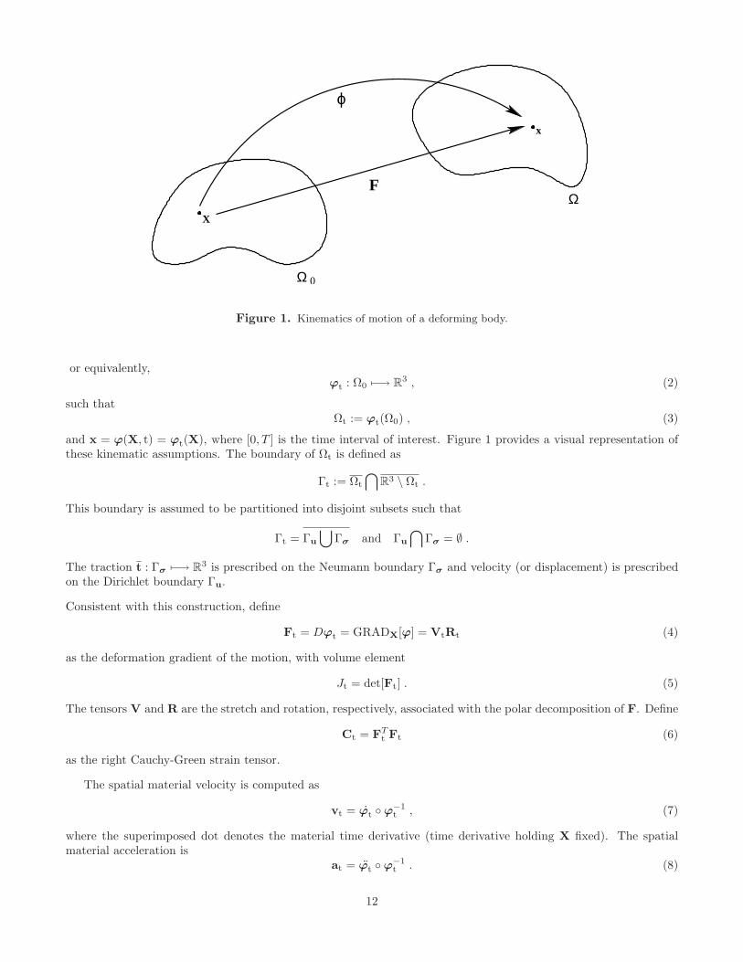
Figure 1. Kinematics of motion of a deforming body.
or equivalently,ϕt : Ω0 7−→ R3 , (2)
such thatΩt := ϕt(Ω0) , (3)
and x = ϕ(X, t) = ϕt(X), where [0, T ] is the time interval of interest. Figure 1 provides a visual representation ofthese kinematic assumptions. The boundary of Ωt is defined as
Γt := Ωt
⋂R3 \ Ωt .
This boundary is assumed to be partitioned into disjoint subsets such that
Γt = Γu
⋃Γσ and Γu
⋂Γσ = ∅ .
The traction t : Γσ 7−→ R3 is prescribed on the Neumann boundary Γσ and velocity (or displacement) is prescribedon the Dirichlet boundary Γu.
Consistent with this construction, define
Ft = Dϕt = GRADX[ϕ] = VtRt (4)
as the deformation gradient of the motion, with volume element
Jt = det[Ft] . (5)
The tensors V and R are the stretch and rotation, respectively, associated with the polar decomposition of F. Define
Ct = FTt Ft (6)
as the right Cauchy-Green strain tensor.
The spatial material velocity is computed as
vt = ϕt ϕ−1t , (7)
where the superimposed dot denotes the material time derivative (time derivative holding X fixed). The spatialmaterial acceleration is
at = ϕt ϕ−1t . (8)
12
Some material models require deformation rate(s) to evaluate their stress response. Towards that end, define
lt = grad[vt] =(FtF
−1t
)ϕ−1
t , (9)
as the spatial velocity gradient anddt = symm[lt] , (10)
as the spatial rate of deformation tensor. The spatial rate of deformation tensor d may be rotated back to thematerial configuration via the transformation
Dt = RTt (dt ϕt) Rt , (11)
thus defining a material rate of deformation tensor. Materials typically undergo both stretch and rotation andmultiple rotation rates may be constructed. For the purposes of this report, define two rotation rates
wt = skew[lt] , (12)
andΩt =
(RtR
Tt
)ϕ−1
t ⇐⇒ Rt = (Ωt ϕt)Rt . (13)
Note that these two rates are in general not the same for arbitrary motions.
2.2 Kinetics
The law of conservation of mass may be written quite simply as follows. Given a material mass density ρ0 : Ω0 7−→ R+,the spatial mass density ρt : Ωt 7−→ R+ is given by
ρt = (J−1t ρ0) ϕ−1
t . (14)
Let σt : Ωt 7−→ R6 denote the symmetric Cauchy stress in the current configuration. Then define
St = JtF−1t (σt ϕt)F
−Tt , (15)
as the second (symmetric) Piola-Kirchhoff stress,
Pt = FtSt , (16)
as the first, and generally unsymmetric, Piola-Kirchhoff stress and
Σt = RTt (σt ϕt)Rt , (17)
as the Cauchy stress rotated back to the material configuration. In many situations it proves convenient to workwith the Kirchhoff stress
τ t := Jtσt = FtStFTt . (18)
Many hypo-elastic material models in Alegra are based upon the use of the Green-McInnis-Naghdi [96] objectivestress rate
σ :=
(Rt
[d
dtΣt
]RT
t
)ϕ−1
t . (19)
Remarks 2.1.
1. The Green-McInnis-Naghdi rate is simply one rate among many. All objective rates are essentially Lie deriva-tives [71]. Hypo-elastic material models require the use of an objective stress rate. However, the choice of whichrate to use is a matter of personal preference or computational convenience. There are no formal mathematicalor rational thermodynamic reasons to prefer one rate over another.
13
2. Reference [104], footnote, page 404: “Various stress rates have been used in the literature. Despite claims andwhole papers to the contrary, any advantage claimed for one such rate over another is pure illusion.”
It proves convenient at this juncture to introduce the L2 inner product(s) as
〈a,b〉t =
∫
Ωt
a • b dΩt , (20)
〈a,b〉Γ =
∫
Γ
a • b dΓ . (21)
With this notation in hand, the weak form of the balance of linear momentum may be written as: find ϕ satisfyingthe boundary conditions on Γu such that for all δϕ
〈δϕ, ρtat〉t +⟨grad(s) δϕ,σt
⟩
t− 〈δϕ, ρtb〉t − 〈δϕ, t〉Γσ
= 0 , (22)
where b is the body-force density per unit mass and t is the prescribed traction on the Neumann boundary Γσ. Thenotation (·)s or (·)(s) indicates the symmetric part of (·). This is often referred to as the principle of virtual workin the spatial configuration [28]. The virtual displacement field δϕ is required to be kinematically admissible in thesense that δϕ vanishes on the Dirichlet boundary Γu. Equation (22) is equivalent to
〈δϕ, ρ0at〉0 + 〈GRADX δϕ,Pt〉0 − 〈δϕ, ρ0b〉0 −⟨δϕ, T
⟩Γ0
σ
= 0 , (23)
where T · dΓ0 := t · dΓt, Γ0 := ϕ−1t (Γt) and Γ0
σ := ϕ−1t (Γσ). This is the principle of virtual work in the reference
(material) configuration [28].
Remarks 2.2. Nansen’s formula [28, 47, 71] states that
n · dΓt = JtF−Tt N · dΓ0 , (24)
where n and N are the unit outward normals to the spatial and material configurations, respectively.
2.3 Balance of energy
Assume there exists an internal energy density function (per unit mass) ε : Ωt −→ R+. The spatial balance of energyequation is ([104], equation 79.3)
ρtε = (σt • dt)− div q + ρtr , (25)
where q : Ωt −→ R3 is the spatial (Cauchy) heat flux and r : Ωt −→ R is the external heat source per unit mass.
3 Discrete Time Integration
For a comprehensive overview of the time-stepping and stress update algorithms used in finite element hydrocodesthe reader is strongly encouraged to review [10]. The notation used in this section is almost exactly that of Section8.1 of [96].
3.1 Incremental kinematics
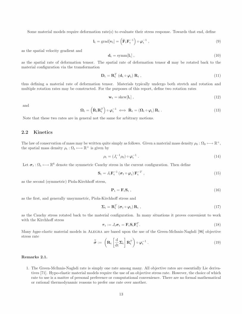
The goal of this subsection is to describe the time-discrete kinematics used in Alegra . Define the midpointconfiguration of the body as the convex combination
ϕn+α = (1− α)ϕn + αϕn+1 for α ∈ [0, 1] . (26)
14
n+α
n+α
n+α
n+α
n+α
n+α
n+α
F
ϕ
X
x
n
n
Ω n
xn+1
Ω 0
ϕn+1 Fn+1 x
F
f
Ω
ϕ
Ω n+1
ϕ ϕn
ϕ ϕ−1n+1
n
−1
Figure 2. Incremental kinematics of motion of a deforming body.
Consistent with this, the midpoint deformation gradient is the convex combination
Fn+α = (1− α)Fn + αFn+1 for α ∈ [0, 1] . (27)
The incremental motion relating the configurations Ωn and Ωn+1 is
φ = ϕn+1 ϕ−1n = id + un+1 , (28)
where id is the identity mapping. By this construction
φ : Ωn −→ Ωn+1 . (29)
The incremental displacement field is defined as
un+1 = (ϕn+1 −ϕn) ϕ−1n . (30)
The displacement field un+1 can be evaluated as a function of xn or as a function of xn+α using the operatorcompositions
un+1 := un+1 ϕn ϕ−1n+α = (ϕn+1 −ϕn) ϕ−1
n+α . (31)
Figure 2 provides a visual representation of these incremental kinematics.
The incremental deformation gradient is defined as
fn+α = gradn[ϕn+α ϕ−1n ] = Fn+αF−1
n , (32)
with an incremental volume elementjn+α = det[fn+α] . (33)
To compute this deformation from the incremental displacement field, notice that
fn+α = (1− α)I + αfn+1 = I + α gradn[un+1] . (34)
15
It is possible to accumulate the total displacement field, if desired. This field is simply the accumulated sum
Un+1 := ϕn+1 −ϕ0 =n∑
i=0
(ϕi+1 −ϕi) =n∑
i=0
ui+1 ϕi (35)
There are at least two ways to compute the total deformation using the total displacement field:
1.Fn+1 = I + GRADX[Un+1]
2.F−1
n+1 = I− gradn+1[Un+1 ϕ−1n+1]
3.Fn+α = GRADX[ϕn+α] = (1− α)Fn + αFn+1
3.2 Central-Difference Method
Alegra uses the central-difference method to integrate in time the continuum dynamics equation(s) of motion.For more detailed information, the reader may consult [7, 62, 110]. Given data Un,vn−1/2,σn, εn, the goal is tocompute un+1,Un+1,vn+1/2,σn+1, εn+1. The time step(s) are defined as
hn+1 = tn+1 − tn;
hn = tn − tn−1;
h =1
2(hn + hn+1)
. (36)
Algorithm Central-Difference. The central-difference method is implemented in eight(8) steps:
1. Solve for the accelerations:
〈δϕ, ρnan〉n +⟨grad(s)
n [δϕ],σn
⟩
n− 〈δϕ, ρnb〉n − 〈δϕ, t〉Γσ
= 0 ∀δϕ , (37)
or equivalently,
〈δϕ, ρ0an〉0 + 〈GRADX[δϕ],Pn〉0 − 〈δϕ, ρ0b〉0 −⟨δϕ, T
⟩Γσ
= 0 ∀δϕ . (38)
2. Modify the accelerations for contact:
(a) Predict the velocity field:
vpredn+1/2 = vn−1/2 + han . (39)
(b) Predict the displacement field(s):
upredn+1 = hn+1v
predn+1/2 , (40)
Upredn+1 = Un + upred
n+1 . (41)
(c) Solve for the contact-induced accelerations: Compute a contact force based on gap-function calculations.The contact force affects the accelerations in that
〈δϕ, ρnac〉n + 〈δϕ, tc〉Γc= 0 ∀δϕ , (42)
where ac is the contact-inducted acceleration and tc is the contact traction on Γc ⊆ Γ \ (Γu
⋃Γσ).
16
(d) Correct the acceleration field: The computed accelerations are modified such that
an+= ac . (43)
3. Update the velocity field:vn+1/2 = vn−1/2 + han (44)
4. Correct the computed velocity field to account for Dirichlet boundary conditions. This essentially involvesresetting the values of vn+1/2 to correspond to known data on any Dirichlet boundaries Γu.
5. Compute the displacement field(s):un+1 = hn+1vn+1/2, (45)
and/or set un+1 directly if the displacement is known on any Dirichlet boundaries Γu. Then simply compute
Un+1 = Un + un+1
ϕn+1 = ϕn + un+1
. (46)
6. Calculate the incremental work done and update the internal energy εn+1 of each material (see Section 5).
7. Given the (corrected) displacement field(s), compute the deformation Fn+1 and compute the stress σn+1. Thisstep is discussed in Section 6.
8. Data swap: Un,vn−1/2,σn, εn ⇐=\ Un+1,vn+1/2,σn+1, εn+1 . Goto one(1).
(End Algorithm Central-Difference)
Remarks 3.1.
1. Step one(1) is only correct assuming the use of a “lumped” mass matrix. If the mass matrix is “consistent”step one(1) must be modified. Let an : Ωn 7−→ R3 be an acceleration field such that an(x) is known if x ison a Dirichlet boundary Γu. (It is entirely possible that an = 0.) Assume the virtual displacement field δϕ is“admissible” in the sense that δϕ = 0 on any Dirichlet boundary Γu. In step one(1) solve
〈δϕ, ρn (an + an)〉n +⟨grad(s)
n δϕ,σn
⟩
n− 〈δϕ, ρb〉n − 〈δϕ, t〉Γσ
= 0 ∀δϕ ,
where an : Ωn 7−→ R3 is zero on all Dirichlet boundaries Γu. The total acceleration is then an = an + an. Thismodification essentially decomposes the acceleration field into two components, one known and one unknown.In step four(4), the velocity correction must be algorithmically consistent with an on Dirichlet boundaries.Note that this of no particular concern since Alegra does in fact use only lumped mass matrices in the soliddynamics algorithms.
2. For frictionless contact, an augmented Lagrangian [42] node-on-surface contact algorithm is used. The detailsare omitted here, but the reader may consult [5, 17, 18, 50] for more information. For simulations withoutcontact step two(2) may be omitted.
3. For purely mechanical problems the central difference algorithm is second-order accurate in time.
4. Notice that the velocities are explicitly computed at times tn−1/2 and tn+1/2. If the velocity at time tn isneeded, it is evaluated as
vn :=1
2
(vn−1/2 + vn+1/2
). (47)
5. In many references [56, 60, 69], the central-difference method is written as1
〈δϕ, ρnan〉n +⟨grad(s)
n δϕ,σn
⟩
n= 0 ∀δϕ
Un+1 = Un + hvn +1
2h2an
vn+1 = vn +1
2h(an + an+1)
, (48)
1For convenience, body forces and applied tractions are omitted.
17
for a time step h > 0. This is equivalent to the form presented in Algorithm Central-Difference, at least for aconstant time step h := hn = hn+1 = h. First, rewrite equation (48)3 as
h2an = 2h(vn+1 − vn)− h2an+1 . (49)
The substitution of this into equation (48)2 produces
Un+1 −Un = hvn+1 −1
2h2an+1 . (50)
The time step index (n) is arbitrary here and thus
Un −Un−1 = hvn −1
2h2an . (51)
The subtraction of equation (51) from equation (48)2 yields
Un+1 − 2Un + Un−1 = h2an . (52)
However, equations (44) - (46) imply
h2an = h(vn+1/2 − vn−1/2)
= (Un+1 −Un)− (Un −Un−1)
= Un+1 − 2Un + Un−1
, (53)
which is the desired result. Both representations produce the same displacement difference stencil. Thisdemonstrates the equivalence of the two alternative representations of the central-difference method.
Remarks 3.2.
1. Many of the material models in Alegra require an approximation of the velocity gradient l = d+w to performconstitutive updates and compute the stress. In Alegra these approximations are
ln+1/2 = gradn+1/2[vn+1/2] , (54)
dn+1/2 = symm[ln+1/2] , (55)
andwn+1/2 = skew[ln+1/2] . (56)
2. Notice thathn+1ln+1/2 = gradn+1/2[un+1]
= gradn[un+1] f−1n+1/2
= gradn[(ϕn+1 −ϕn) ϕ−1n ] f−1
n+1/2
= (fn+1 − I) f−1n+1/2
= 2(fn+1 − I)(fn+1 + I)−1
.
3. Under a superposed rigid body motion (SRBM), ϕn+1 = Qϕn for some Q ∈ SO(3). In this circumstance,dn+1/2 = 0. To see this, notice that in this situation fn+1 = Q,
fn+1/2 =1
2(I + Q),
and thushn+1ln+1/2 = 2(Q− I)(Q + I)
−1.
The reader may easily verify that
symm[(Q + I)
Tln+1/2(Q + I)
]= 0.
Thus ln+1/2 is skew. (See also Corollary 8.1 of [96].)
18
a b
cd
a
bc
d
a
b
c
d ab
c d
a
b
c
d
a
b
c
d
initial
configuration
midpoint
configurations
final
configurations
(collapse)
90
135
180
90
135
1
2
180
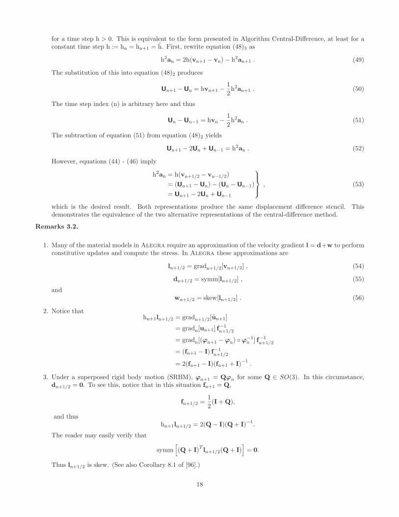
Figure 3. Behavior of the average(midpoint) configuration as a function of rotation. This figure is similarto figure one(1) of reference [57].
4. The immediately preceding analysis ensuring incremental objectivity of ln+1/2 requires that (Q + I) be non-singular. This is equivalent to requiring that −1 not be an eigenvalue of Q. In that pathological case Qrepresents a rotation of π radians and the “average configuration” collapses to a point; see figure 3. Thusthe algorithm for computing l is restricted to rotation increments strictly less than π radians. Fortunately,such a large rotation increment is generally beyond the range of expected values for an explicit time-steppingalgorithm like the central-difference method. More details can be found in [57].
5. There are multiple possibilities for computing the polar decomposition Fn+1/2 = Vn+1/2Rn+1/2. Clearly, oneway is the “DG” method; just compute them directly [51, 52]. Another way is the “VR” method as suggestedby Dienes [35, 39, 62]. The Dienes algorithm is described in excellent detail by reference [41], which includesa flowchart outlining its implementation in an explicit time-stepping scheme. In either case, it is now assumedthat Vn+1/2 and Rn+1/2 are available for use.
4 Spatial Approximation
In almost all regards Alegra uses a standard finite element spatial interpolations. Uniform strain isoparametrictensor product elements transformed from the parent domain [−1, 1]
Ndim are used [7, 8, 40]. These correspond to four-node quadrilateral elements in two dimensions are eight-node hexahedral elements in three dimensions. These are thesimplest (non-locking) elements available for general purpose finite element analysis. Standard nodal shape functionsare used to interpolate continuous fields such as position, velocity and acceleration. Shape function gradients arecalculated by appropriate transformation of natural coordinate gradients [56, 112]. Any needed kinematic tensorfields are computed using the shape function gradients.
For standard finite element analysis,
ϕ =
Nnodes−1∑
A=0
NAϕA =⇒ grad[ϕ] =
Nnodes−1∑
A=0
ϕA ⊗ grad[NA] , (57)
where ϕA is the value of ϕ at node A and the shape function for node A is denoted by NA. The same spatial
19

interpolation is applied to δϕ. Thus equation (37) can be written for node A in matrix form as
Nnodes−1∑
B=0
MABaB + FAint − FA
ext = 0, (58)
where
MAB =
∫
Ωn
ρnNANB dΩn , (59)
is the mass matrix,
FAint :=
∫
Ωn
σn gradn[NA] dΩn , (60)
is the internal force vector at node A and
FAext :=
∫
Ωn
NAρnbn dΩn +
∫
Γn
NAtdΓn , (61)
is the external force vector at node A. If the mass matrix is lumped then
MA :=
Nnodes−1∑
B=0
[∫
Ωn
ρnNANB dΩn
]=
[∫
Ωn
ρnNA dΩn
],
and MAB = MAδAB (no sum on A).
All force integrals in Alegra are evaluated using a “mean quadrature” approach [40]. For example, equation (60)is numerically evaluated using the approximation
FAint ≈ σn
∫
Ωn
gradn[NA] dΩn ,
where σ is the (spatially constant) stress in the element. This stress is calculated using the mean volumetricdeformation, the mean deformation gradient and/or the mean rate of deformation tensor for the element. The meanvalue of a kinematic field (·) in an element Ωe is calculated as
(·) :=1
meas(Ωe)
∫
Ωe
(·) dΩe . (62)
All relevant (thermodynamic) fields, which include but are not limited to, deformation rate, stress, pressure,density and internal energy, are assumed spatially constant in each element. Thus position and velocity are C0(Ω) ⊂H1(Ω) fields defined by nodal values and thermodynamic quantities are L2(Ω) fields defined by piecewise constantelement values. This is often referred to as a staggered grid spatial interpolation [23, 25]. Note also that a givenkinematic field can be non-zero pointwise but may still have a zero mean value. In particular, there exist deformationmodes for four-node planar and eight-node brick elements which have zero mean deformation. To avoid propagationof these zero-energy spurious modes hourglass control (section 8) is required.
Remarks 4.1. Using the divergence theorem, some volume integrals can be converted to surface integrals. Forexample, ∫
Ω
grad[NA] dΩ =
∫
Γ
NAndΓ ,
where Γ is the boundary of Ω and n is the outward normal. This approach to integral evaluation can reduce thetotal number of floating point computations, especially for elements such as the four-node quadrilateral, which hasstraight sides.
5 Energy Calculations
Step six(6) of algorithm central-difference requires a computation of the updated internal energy for each material.This section discusses the method Alegra uses for this update.
20
5.1 Existing Alegra Algorithm
Assuming no external heat sources and adiabatic conditions, equation (25) reduces to
ρtε = (σt • dt) . (63)
One simple way to integrate this numerically is the generalized midpoint rule
ρn+β · (εn+1 − εn) = h(σn+β • dn+β) for β ∈ [0, 1] . (64)
Remarks 5.1.
1. Example material models.
• Ideal gas.σ = −(γ − 1)ρtεI ,
where γ > 1 is the ratio of the specific heats.
• Viscous fluid.σ = 2µdev dt ,
where µ > 0 is the dynamic shear viscosity.
• Hyper-elasticity. See section 6.2.
2. For an element e with domain Ωe ⊆ Ωt,
〈σt,dt〉t = 〈σt, lt〉t
=
⟨σt,
Nnodes−1∑
A=0
vA ⊗ grad[NA]
⟩
t
=
Nnodes−1∑
A=0
⟨vA,σt grad[NA]
⟩t
=
Nnodes−1∑
A=0
vA •[∫
Ωe
σt grad[NA] dΩe
]
=
Nnodes−1∑
A=0
FAint • vA
3. The method above is implicit for β > 0. Alegra currently uses β = 0. Actually, what Alegra really does(for each element) is
εn+1 = εn + h
[∫
Ωn
ρn dΩn
]−1
〈σn,dn〉n
= εn + h
[∫
Ωn
ρn dΩn
]−1[
Nnodes−1∑
A=0
FAint • vA
]
n
= εn + hM−1e
[Nnodes−1∑
A=0
FAint • vA
]
n
.
The total mass of an element e is denoted by Me. (Recall that all stress/strain/energy/density fields areconstant within each cell.) The stress power is computed in UnsDynamics::Calculate_Work() and the energyis updated in UnsDynamics::Update_Density_and_Energy(). Notice that for β = 0 this is an explicit energyupdate, and does not depend on the state of the material at time tn+1, only the state at time tn.
4. Given that Alegra uses β = 0, the algorithm, as implemented, is only first-order accurate. Only the choiceβ = 1/2 is second-order accurate.
21

5.2 Equation(s) of State
For this class of materials assume the stress is simply σ = −pI, where p is the (thermodynamic) pressure. Consistentwith fluid dynamics convention the pressure is assumed positive in compression. Assume there exists an equation of
state such that
p = p(ρ, ε) =⇒ σ = −pI , (65)
for a (smooth) function p : R+ × R+ 7−→ R. For this class of materials, assuming the internal energy density εn+β
(see section 5.1) and the density ρn+β have been computed, the pressure may be updated by a function evaluation
pn+β = p(ρn+β , εn+β) ∀β ∈ [0, 1] . (66)
The update of more complex material models is discussed in Section 6.
Remarks 5.2.
1. The density update is purely kinematic:
ρn+β = det(fn+β)−1
ρn ∀β ∈ [0, 1] .
The density is updated in UnsDynamics::Update_Density_and_Energy().
2. It may be possible to couple equations (65) - (66) with equation (64) for β > 0. This creates a (generally)implicit coupled system of equations for the pressure and the energy. The equations are non-linear and must besolved in some simultaneous iterative fashion [21]. With β = 0 the equations are uncoupled. Again, Alegra
currently uses β = 0.
3. See Ideal_Gas::Update_State(...). In this function it is assumed that εn+1 has already been determined.Thus only the pressure is computed. All equation of state models in Alegra are implemented in this fashion(energy first, pressure second; an explicit, staggered, de-coupled update). See remark (5.1)3.
4. All Alegra material model “updates” (hypo-elastic, hyper-elastic, equation of state, ideal gas...) are drivenby UnsEnergetics::Material_State_Update(). This function is called after density and energy have beenupdated.
5. The reader may find it helpful to review the Alegra equations (for an ideal gas) in one(1) space dimensionusing a finite difference rather than a finite element notation. The one-dimensional stencils can be used forstability analysis, if desired, and are given in Appendix C.
5.3 Conservation Properties
The goal of this section is to discuss the global conservation properties of the Alegra algorithm. Only the caseβ = 0 is considered.
5.3.1 Angular Momentum
In absence of external tractions and body forces, the Alegra algorithm can be written in Lagrangian weak form as
⟨δϕ, ρ0(vn+1/2 − vn−1/2)
⟩0
+ h 〈GRADX[δϕ],FnSn〉0 = 0 ∀ δϕ. (67)
Under suitable (pure Neumann) boundary conditions, an admissible choice for δϕ is δϕ = w×ϕn for some w ∈ R3.A simple substitution yields
⟨w ×ϕn, ρ0(vn+1/2 − vn−1/2)
⟩0
+ h 〈GRADX[w ×ϕn],FnSn〉0 = 0 . (68)
22
Given any vector w ∈ R3, there exists a unique 3 × 3 skew-symmetric tensor w such that w × a = wa ∀a ∈ R3.Using this property, the above equation can be written as
⟨w ×ϕn, ρ0(vn+1/2 − vn−1/2)
⟩0
+ h 〈GRADX[wϕn],FnSn〉0 = 0 . (69)
Consider the second term on the left hand side:
〈GRADX[wϕn],FnSn〉0 = 〈wFn,FnSn〉0=⟨w,FnSnF
Tn ,⟩0
= 0
(70)
since the tensor FSFT is symmetric and w is skew. This leaves only the first term, which by manipulating the crossproduct can be written as ⟨
w,ϕn × ρ0(vn+1/2 − vn−1/2)⟩0
= 0 . (71)
Since the vector w is arbitrary, this yields the conservation statement
∫
Ω0
ϕn × ρ0(vn+1/2 − vn−1/2) dΩ0 =
∫
Ωn
ϕn × ρn(vn+1/2 − vn−1/2) dΩn = 0 . (72)
Remarks 5.3. This conservation statement may seem somewhat odd to the reader. However, it is not inconsistentwith the variational structure of the central difference method [60]. The variational structure of a time integrationscheme guarantees that some momentum-like quantity (a momentum map [72]) is conserved [60, 69]. The conservedquantity is not necessarily intuitive or obvious, but is rather the consequence of a discrete version of Noether’sTheorem [4].
5.3.2 Energy
Definition 5.1. The total kinetic energy is defined as
Tn+α =1
2
∫
Ω0
ρ0‖vn+α‖2 dΩ0. (73)
Definition 5.2. The total internal energy is defined as
Vn+α =
∫
Ω0
ρ0εn+α dΩ0. (74)
In absence of external tractions and body forces, the Alegra algorithm can be written in Lagrangian weak formas ⟨
δϕ, ρ0(vn+1/2 − vn−1/2)⟩0
+ h 〈GRADX[δϕ],Pn〉0 = 0 ∀ δϕ, (75a)
〈ζ, ρ0(εn+1 − εn)〉0 − h〈ζ,Pn •GRADX[vn]〉0 = 0 ∀ ζ, (75b)
with
vn :=1
2(vn−1/2 + vn+1/2) . (76)
Under suitable (pure Neumann) boundary conditions, an admissible choice for δϕ is δϕ = vn. An admissible choicefor ζ is ζ = 1. With these substitutions, the above equations become
Tn+1/2 − Tn−1/2 + ∆W = 0, (77a)
Vn+1 − Vn −∆W = 0, (77b)
with the incremental work done defined as
∆W := h
∫
Ω0
Pn •GRADX[vn] dΩ0 . (78)
Clearly this yields the total energy conservation statement
(Tn+1/2 + Vn+1
)−
(Tn−1/2 + Vn
)= 0. (79)
23
Remarks 5.4.
1. Numerical simulations using Alegra have suggested that the central difference method is mildly unstablefor rapid adiabatic (isentropic) expansion(s) of ideal gases [29, 85]. Please see the continuing remarks whichimmediately follow and also Appendix D.
2. Notice that the energy update equation uses the time step h rather than hn+1. This is necessary to ensurethat a statement of total energy conservation exists. However, the use of the time step h does seem to beinconsistent with the time-centering of the internal energy.
3. One might argue that the above conservation statement is somewhat disconcerting. Notice that the time-centering of the kinetic energy is shifted by a half-step from the time centering of the internal energy. Thisdoes not imply that the conservation statement is invalid or incorrect. Nevertheless, it does bring into questionthe validity of the central difference method for strongly coupled thermo-mechanical continuum problems.
4. The central difference method is a very commonly used time integrator for continuum and structural dynamics.For purely mechanical problems the algorithmic properties are well understood and the method continues to bereliable and effective. However, for strongly coupled thermodynamic problems, the stability and conservationproperties of the algorithm can be brought into question. These issues arise only for thermally (energetically)coupled problems, and not for the purely mechanical case [29, 85].
5. The reason that the choice β = 1/2 is not studied here is because the use of β 6= 0 generally leads to a non-conservative algorithm. The lack of a conserved energy may result in incorrect shock speeds (and thus shocklocations) and a loss of convergence (to weak solutions) for hydrodynamic simulations (see paper [63] and book[101], section 9.6). Convergence to incorrect solutions is also possible [54].
6. An alternative second-order accurate energy update algorithm is proposed in Appendix A. Unfortunately, aconserved total energy quantity does not generally exist for that approach. More significantly, the current Ale-
gra central-difference based algorithm cannot in general achieve linear stability, global second-order accuracy
and conservation of total energy simultaneously [85].
5.3.3 Incremental Objectivity
The goal here is to determine the incremental objectivity properties of the Alegra energy update.
Proposition 5.1. Assume ϕn = Q1ϕn−1 and ϕn+1 = Q2ϕn for some Q1,Q2 ∈ SO(3). Then the energy update isincrementally objective if hn = hn+1 and Q1 = Q2.
Proof. Using the update equations of section 3.2,
ϕn = ϕn−1 + hnvn−1/2
ϕn+1 = ϕn + hn+1vn+1/2
, (80)
under the kinematic assumptions of the proposition gives
vn−1/2 = h−1n (ϕn −ϕn−1) = h−1
n (I−Q1)ϕn−1 = h−1n (I−Q1)Q
T1 ϕn = h−1
n (QT1 − I)ϕn
vn+1/2 = h−1n+1(ϕn+1 −ϕn) = h−1
n+1(I−Q2)ϕn
vn =1
2(vn−1/2 + vn+1/2) =
1
2
[h−1
n (QT1 − I) + h−1
n+1(I−Q2)]ϕn
. (81)
Taking the material gradient of the velocity at time tn results in
GRADX[vn] =1
2
[h−1
n (QT1 − I) + h−1
n+1(I−Q2)]Fn . (82)
Now recall the incremental work done (78)
∆W := h
∫
Ω0
Pn •GRADX[vn] dΩ0 = h
∫
Ω0
Sn • FTn GRADX[vn] dΩ0 . (83)
24
Since S is symmetric, a sufficient condition for ∆W = 0 is that FTn GRADX[vn] be skew. This is satisfied if and only
if the quantityh−1
n (QT1 − I) + h−1
n+1(I−Q2) ,
is skew. This is satisfied in general only when hn = hn+1 and Q1 = Q2.
Remarks 5.5.
1. The energy update is guaranteed incrementally objective only when hn = hn+1 and Q1 = Q2. Unfortunately,these are rather restrictive requirements and in general the energy update is not objective. In particular, a rigidbody motion which occurs in a single time step does not generally produce zero incremental work done.
2. Incremental objectivity is not required for consistency, stability or convergence. However, it is a desirableproperty. Consider a continuum body rotating rigidly. If the energy update is not incrementally objective theinternal energy of the material will change as the body rotates. Consequently, for an equation of state modelthe thermodynamic pressure will also change. The result in this case is spurious pressure variations when thepressure should remain constant in time.
Remarks 5.6.
1. Notice that time centering of the data Z := v,x,σ, ε is staggered in a “leap-frog” fashion for the central-difference method. The velocity v and momentum are time located at the mid-points of a time interval, whilethe position x and energy ε are located at the end-points of a time interval. This makes the definition ofalgorithmic quantities such as total energy and total momentum somewhat difficult.
2. The resolution of the energy consistency issues discussed in this report may necessitate the use of an entirelydifferent conservative time integration algorithm. A mid-point based predictor multi-corrector integrator hasshown promise in this regard [93, 94]. That algorithm conserves total angular momentum and an algorithmicallyconsistent and well defined total energy, and is incrementally objective in both stress and energy updates.
3. All data for the mid-point time integrator is centered at the end-points of a time interval. The integrator isimplicitly a map from Zn 7→ Zn+1. In fact, the algorithm can be written abstractly as
Zn+1 = Zn + hn+1 · F(Zn+1/2,hn+1) ,
for an appropriately defined function F. Algorithmic quantities such as total energy and total momentum areeasily defined. The details are in references [93, 94].
6 Stress Update Algorithm
Step seven(7) of algorithm central-difference requires a computation of the updated stress response of the material.The method for performing the constitutive update depends upon the type of material being used.
6.1 Hypo-Elasticity
The concept of hypo-elasticity was originally introduced by Truesdell [103]. More details can be found in [11, 98,104]. Assume a constitutive model of the form
Σt = CDt , (84)
where the rank-four tensor C is positive-definite (coercive) in the sense that
∃κ > 0 such that ∀v,w ∈ R3 (v ⊗w) • C (v ⊗w) > κ‖v‖2‖w‖2 . (85)
Let β ∈ [0, 1]. The algorithm is as follows [96]:
25
1. Compute the material rate of deformation:
Dn+β = RTn+βdn+βRn+β
2. Compute the material stress:
Σn = RTnσnRn
3. Update the material stress:
Σn+1 = Σn + hn+1CDn+β
4. Rotate forward to get Cauchy stress:
σn+1 = Rn+1Σn+1RTn+1
Remarks 6.1.
1. Assume that dn+β is incrementally objective. Then the algorithm above is incrementally objective. Given theway Alegra computes the rate of deformation tensor, only the choice β = 1/2 is incrementally objective.
2. Even with the choice β = 1/2, under a SRBM fn+1 = Q ∈ SO(3), the Cauchy stresses will transform exactlyas σn+1 = QσnQT if and only if Rn+1R
Tn = Q. The Dienes algorithm [35, 41, 62] only approximates this
condition and does not exactly reproduce Q as the incremental rotation.
3. Residual stresses may remain at the end of a closed strain path for hypo-elastic materials [61, 90].
4. General models of hypo-elasticity are incompatible with the notion of hyper-elasticity [11, 98, 104]. More pre-cisely, given a hypo-elastic material model, there does not generally exist a corresponding Helmholtz free energyfunction for that model. Thus the model lacks a solid mathematical basis relative to rational thermodynam-ics [1, 30, 31, 102] and quantities such as internal energy and heat production are ill-defined. The extension ofthis class of material models to the full thermo-elastic regime remains unclear.
5. Hypo-elastic models remain in common use in many commercial and government computational software ap-plications [49, 62]. However, most if not all academic researchers in computational mechanics have long sinceabandoned hypo-elasticity in favor of thermodynamically consistent models of material behavior.
6. The use of a hypo-elastic material model does not guarantee that the continuum evolution equations define an(infinite-dimensional) Hamiltonian system. A Lagrangian action integral is not well defined and as such thevariational structure of the central-difference method is undetermined in this case.
6.2 Hyper-Elasticity
Given the thermodynamic issues associated with hypo-elasticity, one might want to consider alternative models ofmaterial behavior. From a rigorous thermodynamic perspective, hyper-elasticity is more correct; hypo-elasticity hasproven useful, but remains problematic thermodynamically. For a comprehensive overview of continuum thermody-namics the reader may consult [34, 71, 104].
Let Θ > 0 be the absolute temperature field. Given a Helmholtz free energy density Ψ(C,Θ) (per unit mass) [1,30, 31, 71, 104]
Sn+α = 2ρ0
[∂Ψ
∂C
]
C,Θ=Cn+α,Θn+α
. (86)
Then simply
σn+α = J−1n+αFn+αSn+αFT
n+α . (87)
This holds ∀α ∈ [0, 1].
Remarks 6.2.
26

1. There is essentially no need for objective stress rates relative to hyper-elasticity. The material model is purely“strain-driven,” and stresses can be computed and updated directly from the total deformation Fn+1 (or theincremental deformation fn+1) and the time step hn+1 > 0. This is true even with visco-elastic, visco-plasticand damage extensions.
2. The use of a hyper-elastic material model (under the assumption of constant temperature, or alternativelyconstant entropy [104]) ensures that the continuum evolution equations define an (infinite-dimensional) Hamil-tonian system. In this situation, the central-difference method is a variational time integrator [60, 69]. Thetime-discrete equations of the method can be derived as the Euler-Lagrange equations of a time-discrete La-grangian action integral. Subject to time step restrictions, the method possesses rather remarkable stabilityand conservation properties.
3. Thermo-Elasticity [1, 2, 32, 46, 71, 76, 97]:
Internal Entropy Density (per unit mass) :
η = −∂ΘΨ(C,Θ) (88)
Internal Energy Density (per unit mass) :
ε = ε(C,Θ) = Ψ(C,Θ) + η(C,Θ) ·Θ . (89)
ThermoElastic Heating:
H = −1
2Θ · ∂Θ(S • C) = −Θ ·
[ρ0(∂ΘCΨ) • C
](90)
Specific Heat (per unit mass):c := −Θ · ∂2
ΘΘΨ (91)
Heat Conduction:
(a) Entropy form:ρ0Θη = [−J div q + ρ0R] (92)
(b) Temperature form:ρ0cΘ = −H + [−J div q + ρ0R], (93)
where q is the spatial (Cauchy) heat flux and R is the external heat source per unit mass. In general thespecific heat c > 0 is not constant.
4. Note that an equation-of-state model may be considered a special case of thermo-elasticity. Once the updateddensity and internal energy are calculated, the (thermodynamic) pressure is computed by a function evaluation(see Section 5.2). More abstractly, for an equation-of-state model the free energy is assumed to be function ofvolume and temperature Ψ(detC,Θ).
5. Ideal gas. Consistent with the immediately preceding remark, an ideal gas is in fact a type of thermo-elasticmaterial. The internal energy of an ideal gas is given by
ε(ρ, η) = ε0
[ρ
ρ0exp
(η − η0
R
)](γ−1)
, (94)
where R > 0 is the gas constant, γ > 1 is the adiabatic exponent and ρ0, η0, ε0 is the reference state of thegas [77]. A standard sequence of thermodynamic arguments yields (see chapter 2 of [33])
p = ρ2∂ρε =⇒ p = (γ − 1)ρǫ ,
andΘ = ∂ηε =⇒ Θ = c−1
v ε ,
27
where cv = (γ − 1)−1R is the constant volume specific heat capacity per unit mass. This equation may beinverted in closed form as
η − η0 = R log
[ρ0
ρ
(cvΘ
ε0
) 1γ−1
], (95)
and thus
Ψ(ρ,Θ) = ε (ρ, η(ρ,Θ)) − η(ρ,Θ) ·Θ .
Note also that ρ0/ρ = (detC)1/2.
6. As another example, consider a volumetric-deviatoric uncoupled thermoelastic material. In this case, a simpleform for the free energy is [97]
Ψ(C,Θ) = T (Θ) + M(J,Θ)︸ ︷︷ ︸thermal
+ W (C) + U(J)︸ ︷︷ ︸elastic
,
where C := J−2/3C. For a neo-hookean model, these functions may take the form
T (Θ) = c0
[(Θ−Θ0)−Θ log
(Θ
Θ0
)]
M(J,Θ) = −3β(Θ−Θ0)U′(J)
W (C) =1
2ρ−10 µ [trace(C)− 3]
U(J) = ρ−10 κ
[1
2(J2 − 1)− log(J)
]
,
where Θ0 > 0 is the reference temperature, c0 > 0 is the reference heat capacity, β > 0 is the (linearized)coefficient of thermal expansion, κ > 0 is the (linearized) bulk modulus and µ > 0 is the (linearized) shearmodulus.
7. For non-dissipative materials, which include ideal gas and other equation of state models, the use of equa-tion (63), ignoring heat fluxes and heat sources (and artificial viscosity), implies an isentropic process. Fornon-dissipative materials heat conduction
γcon := − 1
ρΘ2(q • grad Θ) > 0 ,
is the only source of local entropy production [30, 32, 34, 104]. For hyper-elasticity, see remark (6.2)8.
8. For hyper-elastic materials assume that the internal energy density ε is a function of deformation and temper-ature (see [104], section 82),
ε = ε(C,Θ) = Ψ(C,Θ) + η(C,Θ) ·Θ ,
where Ψ is the (Helmholtz) free energy density and η is the specific entropy, both per unit mass. Then it shouldbe possible, given εn+1, to solve for Θn+1 implicitly by solving
εn+1 − ε(Cn+1,Θn+1) = 0 .
This is equivalent to numerically approximating adiabatic (and thus isentropic) thermo-elasticity; see equa-tion (92).
9. For general hypo-elastic (section 6.1) material models an internal energy function does not exist. A discussionof dissipation and/or entropy production is meaningless.
28
7 Shock Capturing
7.1 Background information
In shock physics calculations, physical viscosity2 is truly negligible and has space and time scales much smallerthan those resolved by the grid. The weak, or integral, Euler equations are inherently ill-posed (having an infinitenumber of solutions). Computational solutions involving shocks, without some form of stability control, usually havesevere oscillations because of this. Mathematically, it is common practice to add a viscosity term to shock equationsand consider the unique solution arising in the limit as the viscosity vanishes. This approach is known as viscositysolutions. Computationally, a similar effect can be achieved by use of an artificial viscosity to stabilize the computedsolution about a shock [64].
Like physical viscosity, artificial viscosity appears in both the fluid momentum and energy equations through thestress tensor. In the momentum equation the artificial viscosity stress, σav, should act to reduce momentum at theshock front, and hence also reduce the kinetic energy there. In the energy equation, the kinetic energy lost should bedissipated (and entropy produced [32]) by raising the fluid internal energy (σav •d > 0). Thus, like physical viscosity,artificial viscosity acts to convert kinetic energy into internal energy at the shock front. To form an artificial viscositystress tensor, one must construct artificial analogs of physical terms such as µ ∝ ρvthλ and d.
7.2 Standard Artificial Viscosity
The basic von Neumann-Richtmyer artificial viscosity [106] idea is to exchange the space and time scales from thephysical viscosity for ones applicable to the grid and fluid velocity. They replaced the term vthλ in µ with the productof a term proportional to the spatial gradient of the velocity and a space-scale squared. The space-scale is selectedto be a grid length, resulting in a compact smearing of the shock. This basic idea,
σvisc,quad =(ρh2‖d‖
)· ‖d‖ ←− (ρvthλ) ‖d‖ , (96)
results in a term quadratic in the velocity gradient. In multidimensional applications, the simplest approach is touse a scalar coefficient and to compute ‖d‖ as trace[d], independent of shock direction (since evaluating the shockdirection robustly remains an open problem). This simplest application in multiple space dimensions is what Alegra
uses for its quadratic term,
σvisc,quad,ALEGRA = Qquad =(ρl2 |trace[d]|
)· trace[d] · I , (97)
where l > 0 is what Nevada calls the aspect ratio (an element characteristic length scale).
This term is quadratic in d, whereas the physical viscous stress is only linear in d. The second d in the quadraticterm really serves only to help define the space and time scales over which the artificial viscosity acts. An alternativeis to use the sound speed cs > 0 to obtain those space/time scales. This results in the linear term used in Alegra
σvisc,lin,ALEGRA = Qlin = (ρlcs) trace[d] · I . (98)
Thus the final form for the standard artificial viscosity used in Alegra is
σvisc = ρ(
c1lcs + c2l2 |trace[d]|
)trace[d] I , (99)
where c1 > 0 is the linear constant and c2 > 0 is the quadratic constant. This is the general linear plus quadraticform most commonly used in shock hydrodynamics calculations [9, 22, 26, 37, 78, 108].
Remarks 7.1.
2The physical dynamic viscosity coefficient µ ∝ ρvthλ is proportional to the product of the density, the thermal speed (vth ∝√
Θ)and the molecular collision mean free path λ.
29

1. For the compressible Euler equations, the standard Galerkin finite element solution conserves total entropy [55].Without an additional numerical entropy production mechanism, the standard Galerkin method cannot cor-rectly capture shocks and will not converge to an entropy satisfying solution of the Euler equations in thepresence of shocks.
2. Viscous stresses are a source of dissipation and entropy production [32, 104].
3. Based on the theory presented in [75], the artificial viscosity should be explicitly material dependent. Note thatthe linear term of equation (99) depends on the sound speed of the material, but unfortunately the quadraticterm does not.
7.3 Calculation of the rate of deformation
In order to be consistent with the central-difference method, the artificial shock capturing viscous stresses shouldbe computed at time tn+1. This requires an approximation to dn+1, which has not been previously discussed. Thefollowing definitions prove useful in this regard:
Definition 7.1. The pull-back [7] of a rank-two contravariant spatial tensor τ is
ϕ∗τ := F−1τ F−T . (100)
The corresponding push-forward of a contravariant material tensor S is denoted by ϕ∗S.
Definition 7.2. The pull-back [7] of a rank-two covariant spatial tensor g is
ϕ∗g := FT gF . (101)
The corresponding push-forward of a covariant material tensor G is denoted by ϕ∗G.
Definition 7.3. The rate of deformation tensor d is one-half the Lie derivative of the spatial metric g [7]. Moreprecisely, 2d = Lv[g], where
Lv[g] = ϕ∗
(d
dtϕ∗g
). (102)
Without any significant loss of generality, the spatial metric is henceforward assumed to be the identity g = I.
Given these definitions, the rate of deformation d my be computed as
2d = Lv[ I ]
= F−T
[d
dt(FT IF)
]F−1
= F−T CF−1
. (103)
Inverting this equation yieldsC = 2FT dF
= 2FT dF−T C
= 2[FT dF−T
]C
. (104)
A backward-Euler exponential approximation in time of equation (104) produces
Cn+1 ≈ exp[2hn+1F
Tn+1dn+1F
−Tn+1
]Cn
= FTn+1 exp[2hn+1dn+1]F
−Tn+1Cn
. (105)
Inverting this equation yields
exp[2hn+1dn+1] = F−Tn+1Cn+1C
−1n FT
n+1
= F−Tn+1F
Tn+1Fn+1F
−1n F−T
n FTn+1
= (Fn+1F−1n )(Fn+1F
−1n )
T
= fn+1fTn+1
. (106)
30
The end result is
dn+1 =1
2hn+1log[fn+1f
Tn+1] . (107)
Lemma 7.1. det[expA] = exp[traceA] for all n× n matrices A.
Proof. First, assume A is diagonalizable. Then there exists an invertible matrix S and a diagonal matrix D suchthat A = SDS−1. In this case, expA = S[expD]S−1 and det[expA] = det[expD]. However, for a diagonal matrixthis determinant is simply the product of the exponential of the eigenvalues λk
det[expA] = det[expD]
=
n−1∏
k=0
exp(λk)
= exp
[n−1∑
k=0
λk
]
= exp[traceD]
= exp[traceA] .
The proof is completed by noting that diagonalizable matrices are a dense subset of all matrices.
Proposition 7.2. The derived approximation for dn+1 is both incrementally objective and volume preserving.
Proof. Incremental objectivity is satisfied by construction. Alternatively, it follows from the fact that log I = 0. Asfor volume preservation,
j2n+1 = det[fn+1f
Tn+1]
= det(exp[2hn+1dn+1])
= exp[2hn+1 · tracedn+1] .
Thus jn+1 = 1 if and only if tracedn+1 = 0.
Remarks 7.2.
1. The Alegra shock capturing artificial viscosity can be turned on/off in tension (trace[d] > 0), if desired. Theviscosity is always on in compression (trace[d] < 0).
2. See PRONTO_Artificial_Viscosity::Update_Artificial_Viscosity(...).
3. The present default implementation of Alegra uses dn+1/2 rather than dn+1 to compute the artificial viscositypressure. This may not be consistent with the central-difference method.
4. This logarithmic option my be turned on by typing LOGARITHMIC = ON.
7.4 Tensor Artificial Viscosity
A tensor artificial viscosity can help stabilize mesh deformation in some circumstances [22, 80, 91, 93]. Based on theresults presented in [93], a tensor artificial viscosity may be computed as
σvisc := ρνd, (108)
where ν > 0 is the kinematic viscosity. The kinematic viscosity is computed as
ν := c1 cs l + c2 | trace(d)| l2, (109)
where c1 > 0 is the linear constant, c2 > 0 is the quadratic constant, l > 0 is a mesh-based characteristic length scaleand cs > 0 is the sound speed of the material.
31
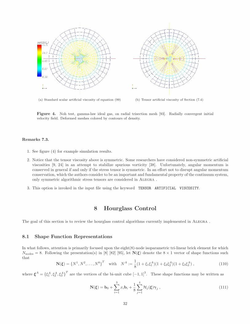
(a) Standard scalar artificial viscosity of equation (99) (b) Tensor artificial viscosity of Section (7.4)
Figure 4. Noh test, gamma-law ideal gas, on radial trisection mesh [93]. Radially convergent initialvelocity field. Deformed meshes colored by contours of density.
Remarks 7.3.
1. See figure (4) for example simulation results.
2. Notice that the tensor viscosity above is symmetric. Some researchers have considered non-symmetric artificialviscosities [9, 24] in an attempt to stabilize spurious vorticity [38]. Unfortunately, angular momentum isconserved in general if and only if the stress tensor is symmetric. In an effort not to disrupt angular momentumconservation, which the authors consider to be an important and fundamental property of the continuum system,only symmetric algorithmic stress tensors are considered in Alegra .
3. This option is invoked in the input file using the keyword TENSOR ARTIFICIAL VISCOSITY.
8 Hourglass Control
The goal of this section is to review the hourglass control algorithms currently implemented in Alegra .
8.1 Shape Function Representations
In what follows, attention is primarily focused upon the eight(8)-node isoparametric tri-linear brick element for whichNnodes = 8. Following the presentation(s) in [8] [82] [95], let N(ξ) denote the 8 × 1 vector of shape functions suchthat
N(ξ) = N1, N2, . . . , N8T with NA :=1
8(1 + ξ1ξ
A1 )(1 + ξ2ξ
A2 )(1 + ξ3ξ
A3 ) , (110)
where ξA = ξA1 , ξA
2 , ξA3
Tare the vertices of the bi-unit cube [−1, 1]
3. These shape functions may be written as
N(ξ) = b0 +
3∑
i=1
xibi +1
8
4∑
j=1
Hj(ξ)γj , (111)
32
where H(ξ) are the hourglass functions defined as
H1(ξ) := ξ2ξ3 , H2(ξ) := ξ3ξ1 , H3(ξ) := ξ1ξ2 , H4(ξ) := ξ1ξ2ξ3 . (112)
The twelve(12)-dimensional hourglass deformation space of the eight-node brick is defined as
H12 := spanH1,H2,H3,H4 × R3 . (113)
This space may be viewed as consisting of four(4) hourglass modes, where each mode can act in any one of three(3)coordinate directions.
The constant 8× 1 vectors b0, bi and γj can be determined in a relatively straight-forward manner. Evaluation
of equation (111) at the nodes of the bi-unit cube and use of the Kronecker property NA(ξB) = δAB yields the 8× 8matrix expression
I8 = b0 ⊗ 18 +
3∑
i=1
bi ⊗ xi +1
8
4∑
j=1
γj ⊗ hj . (114)
In this equation I8 is the 8 × 8 identity matrix, xi = x1i , x
2i , . . . , x
8i
Tis the 8 × 1 vector of nodal coordinates for
component i and
18 := 1, 1, 1, 1, 1, 1, 1, 1T
h1 := 1, 1,−1,−1,−1,−1, 1, 1T
h2 := 1,−1,−1, 1,−1, 1, 1,−1T
h3 := 1,−1, 1,−1, 1,−1, 1,−1T
h4 := −1, 1,−1, 1, 1,−1, 1,−1T
. (115)
The reader may easily verify that 18 •hj = 0 and hj •hk = 8δjk. The multiplication of equation (114) by the vector18 yields the equation
b0 =1
8
[18 −
3∑
i=1
(18 • xi)bi
]. (116)
The multiplication of equation (114) by the vector hk yields the equation
γj =
[hj −
3∑
i=1
(hj • xi)bi
]. (117)
Taking the derivative of (111) with respect to xk (or, alternatively, ξk) and evaluation at the element center ξ = 0yields
bi =3∑
j=1
(J−T
0
)ij
∂N
∂ξj(0) where J0 :=
∂x
∂ξ(0) . (118)
Since bi are consistently computed ’strain-displacement’ operators, one can show that (see [56], chapter 3)
bi • 18 = 0 and bi • xj = δij . (119)
Given these properties, it must also hold from (117) that
γi • 18 = 0 and γi • xj = 0 , (120)
and thus the vectors γi are orthogonal to the homogeneous deformation modes of the tri-linear brick element. Finally,
33
note that in nodal components
γj(A) = hj(A) −3∑
i=1
(hj • xi)bi(A)
= hj(A) −3∑
i=1
(bi(A) ·
Nnodes∑
B=1
hj(B)xi(B)
)
=: hj(A) − bA •Nnodes∑
B=1
hj(B)xB
=: hj(A) − bA • yj
, (121)
where
bA := J−T0 GRADξ[N
A(0)] and yj :=
Nnodes∑
B=1
hj(B)xB . (122)
Remarks 8.1.
1. For a four node quadrilateral element there is only one(1) hourglass function H(ξ) := ξ1ξ2 and one(1) hourglass
vector h = 1,−1, 1,−1T . All the other developments above remain essentially unchanged. The details areomitted.
2. In actual numerical implementations of two(2)-dimensional problems in Alegra , the hourglass vector h isnormalized so that ‖h‖ = 1. In three(3)-dimensional simulations, this normalization is not performed and‖hi‖ =
√8.
8.2 Hourglass Rates
Let vh(A) for A ∈ 1, 2, . . . , Nnodes denote the nodal velocity field of a finite element. Consistent with the develop-ments in [7] [8] [40] [107], define the hourglass rate for mode m as
rhgm :=
Nnodes∑
A=1
γm(A)vh(A) . (123)
8.3 Hourglass Resistance
The goal here is to compute, based on the hourglass rates rhgm , a reasonable value of the hourglass resistance fhg
m .
8.3.1 Pisces
Based on the work in [44], the hourglass resistance for an element e is computed as
fhgm :=
[(2− 1
2Ndim
)· νhg · cs ·
ρ ·meas(Ωe)
he
]· rhg
m , (124)
where Ndim ≥ 2 is the number of spatial problem dimensions, he > 0 is an element characteristic length scale, cs > 0is the maximum material wave speed (ideally determined from an eigenvalue analysis of the acoustic tensor [104])and νhg > 0 is a user defined parameter.
34
8.3.2 Pronto
The Pronto [62] hourglass viscosity coefficient is given by
µhg :=
νhg ·
√128.0 ·G · ρ ·meas(Ωe) if 2-D
νhg ·√
1.5 ·G · ρ · (meas(Ωe))2h−2
e if 3-D, (125)
where G > 0 is the (linearized) shear modulus of the material and νhg > 0 is a user defined parameter. The Prontohourglass control also has the option to time integrate the hourglass ’rate’ to determine an hourglass “stiffness”. ThePronto hourglass stiffness coefficient is given by
κhg :=
khg · 0.5 ·G ·meas(Ωe) · h−2
e if 2-D
khg · 0.125 ·G ·meas(Ωe) · h−2e if 3-D
, (126)
where khg > 0 is a user defined parameter.
Definition 8.1. The pull-back of a spatial one-form (co-vector) ω is defined as
ϕ∗ω := FT ω , (127)
with corresponding push-forward operation ϕ∗ω (see section 1.2 of [71]).
Definition 8.2. The Lie derivative of a spatial one-form ω is defined as
Lv[ω] = ϕ∗
(d
dtϕ∗ω
). (128)
Define a time-integrated “stiffness” parameter shgm for mode m such that
Lv
[shgm
]= F−T d
dt
(FT shg
m
)= khgr
hgm . (129)
A simple approximation in time yields
Lv
[shgm
]≈ F−T
n+1
[FT
n+1shgm (tn+1)− FT
n shgm (tn)
]h−1
n+1
= h−1n+1
[shgm (tn+1)− F−T
n+1FTn shg
m (tn)]
= h−1n+1
[shgm (tn+1)− f−T
n+1shgm (tn)
]
. (130)
This results in the discrete update equation
shgm (tn+1) = f−T
n+1shgm (tn) + hn+1khgr
hgm . (131)
Finally, the hourglass resistance is computed as
fhgm := µhgr
hgm + shg
m . (132)
Remarks 8.2.
1. Clearly the Pronto hourglass control cannot be used for a frictionless material, in particular for frictionlessgases, since the shear modulus G = 0.
2. The Lie derivative is an objective rate and the Pronto stiffness update algorithm is by construction incrementallyobjective.
3. The Pronto stiffness algorithm is implicitly equivalent to using a hypo-elastic material model for hourglassstabilization. Consistent with that, residual hourglass forces may remain at the end of a closed strain path [58].
35
8.4 Hourglass Nodal Forces
Let Fhgm (A) for A ∈ 1, 2, . . . , Nnodes denote the nodal hourglass force field for mode m of a tri-linear brick element.
Once the hourglass resistance has been determined, the nodal forces for hourglass mode m are simply computed as
Fhgm (A) = γm(A) · fhg
m . (133)
8.5 Proposed alternative algorithm
There may be an alternative, albeit more computationally expensive, hourglass control algorithm. For an element ewith domain Ωe ⊆ Ω, define the mean value of the rate of deformation tensor as
d :=1
meas Ωe
∫
Ωe
d dΩe , (134)
and the fluctuation from this mean asd := d− d . (135)
For hourglass control purposes, an artificial viscous stress of the form
σhg := ρνd (136)
can be added to the physical (and shock capturing) stress. In this equation, ν > 0 is a kinematic viscosity, whichmay be computed as
ν = chgcs he , (137)
with chg > 0 an hourglass control parameter. The nodal forces (for node A) associated with this stabilization arecomputed as
Fhg(A) :=
∫
Ωe
σhg grad[NA] dΩe . (138)
Remarks 8.3.
1. This hourglass control algorithm passes the patch test by construction. For a homogeneous deformation, d = 0.
2. This algorithm requires full quadrature to stabilize hourglass modes. The non-homogeneous component d ofthe deformation must be sampled at multiple points, not just at the element center, to fully detect hourglassmodes.
3. The scaling of the hourglass resistance in this approach is similar to that of the Pisces algorithm equation (124).
4. A variational multi-scale based hourglass control algorithm, similar in concept to the one proposed here, isdiscussed in [93, 94].
9 Closure
This report has presented the algorithmic details of the Alegra continuum hydrodynamics package. The packageuses a Galerkin finite element spatial discretization and an explicit central-difference stepping method in time. Thedetails of the algorithm have been presented, along with its strengths and weaknesses. Some suggestions for furtherimprovements and modifications have also been included. It is hoped that this report can help code developers andphysics analysts more easily understand and modify Alegra .
The development and refinement of Alegra is ongoing. Some suggestions for future research and developmentinclude, but are not limited to, the following:
36
• Implementation of a truly second-order, (linearly) stable, conservative predictor multi-corrector time-steppingalgorithm.
• The use of a limiter with the full tensor artificial viscosity to detect isentropic compression and reduce theviscosity smoothly to zero(0) in the absence of shocks.
• Implementation and use of thermodynamically consistent hyperelastic-based solid models for plasticity andfailure.
• The coupling of X-FEM (see [105] and references therein) to the existing Lagrangian scheme to enable a bettertreatment of multi-material problems.
• Investigation into alternative spatial discretizations for Lagrangian shock hydrodynamics, including continuouspressure SUPG-stabilized formulations [92] and H(div) finite elements [3, 6, 12, 14, 15, 86, 87]. H(div) formu-lations are not typically used for Lagrangian hydrodynamics, but recent research has shown promise in thatregard [83, 88].
Acknowledgment: The authors wish to thank Dr. Allen C. Robinson and Dr. Randall M. Summers for theircontinuing support and encouragement. The authors thank Dr. Allen C. Robinson, Dr. William J. Rider andDr. Joshua Robbins for reviewing initial drafts of the report. The authors also thank Dr. William J. Rider andDr. Guglielmo Scovazzi for helpful discussions. Mr. Kyle Cochrane very kindly provided the numerical simulation ofAppendix D.
References
[1] Stuart S. Antman. Nonlinear problems of elasticity, volume 107 of Applied Mathematical Sciences. Springer,New York, 2nd edition, 2005.
[2] F. Armero and J. C. Simo. A new unconditionally stable fractional step method for non-linear coupled thermo-mechanical problems. International Journal for Numerical Methods in Engineering, 35(4):737–766, September1992.
[3] Douglas N. Arnold, Daniele Boffi, and Richard S. Falk. Quadrilateral H(div) finite elements. SIAM Journal
on Numerical Analysis, 42(6):2429–2451, 2005.
[4] V. I. Arnold. Mathematical Methods of Classical Mechanics, volume 60 of Graduate Texts in Mathematics.Springer, New York, 2nd edition, 1989.
[5] S. W. Attaway, B. A. Hendrickson, S. J. Plimpton, D. R. Gardner, C. T. Vaughan, K. H. Brown, and M. W.Heinstein. A parallel contact detection algorithm for transient solid dynamics simulations using PRONTO3D.Computational Mechanics, 22(2):143–159, August 1998.
[6] C. Bahriawati and C. Carstensen. Three matlab implementations of the lowest-order Raviart-Thomas MFEMwith a posteriori error control. Computational Methods in Applied Mathematics, 5(4):333–361, 2005.
[7] Ted Belytschko, Wing Kam Liu, and Brain Moran. Nonlinear finite elements for continua and structures. JohnWiley and Sons, New York, 2000.
[8] Ted Belytschko, Jame Shau-Jen Ong, Wing Kam Liu, and James M. Kennedy. Hourglass control in linear andnonlinear problems. Computer Methods in Applied Mechanics and Engineering, 43(3):251–276, May 1984.
[9] David J. Benson. A new two-dimensional flux-limited shock viscosity for impact calculations. Computer
Methods in Applied Mechanics and Engineering, 93(1):1991, December 1991.
[10] David J. Benson. Computational methods in lagrangian and eulerian hydrocodes. Computer Methods in Applied
Mechanics and Engineering, 99(2-3):235–394, September 1992.
37
[11] Barry Bernstein. Hypo-elasticity and elasticity. Archive for Rational Mechanics and Analysis, 6(1):89 – 104,January 1960.
[12] Pavel B. Bochev, Jonathan J. Hu, Allen C. Robinson, and Raymond S. Tuminaro. Towards robust 3d Z-pinchsimulations: discretization and fast solvers for magnetic diffusion in heterogeneous conductors. Electronic
Transactions on Numerical Analysis, 15:186–210, 2003.
[13] Javier Bonet and Richard D. Wood. Nonlinear Continuum Mechanics for Finite Element Analysis. CambridgeUniversity Press, September 1997.
[14] Franco Brezzi and Michel Fortin. Mixed and Hybrid Finite Element Methods, volume 15 of Springer Series in
Computational Mathematics. Springer-Verlag, New York, 1991.
[15] Franco Brezzi, Jim Douglas Jr., and L. D. Marini. Two families of mixed finite elements for second orderelliptic problems. Numerische Mathematik, 47(2):217–235, June 1985.
[16] Alexander N. Brooks and Thomas J.R. Hughes. Streamline upwind/petrov-galerkin formulations for convectiondominated flows with particular emphasis on the incompressible navier-stokes equations. Computer Methods
in Applied Mechanics and Engineering, 32(1-3):199–259, September 1982.
[17] Kevin H. Brown, Michael W. Glass, Arne S. Gullerud, Martin W. Heinstein, Reese E. Jones, and Randall M.Summers. ACME : a parallel library of algorithms for contact in a multi-physics environment. In K. J. Bathe,editor, Proceedings of the First MIT Conference on Computational Fluid and Solid Mechanics, ComputationalFluid and Solid Mechanics, Cambridge, Massachusetts, June 2001. Massachusetts Institute of Technology,Elsevier. Sandia Report SAND2001-0904A.
[18] Kevin H. Brown, Martin W. Heinstein, Reese E. Jones, and Thomas E. Voth. Explicit transient dynam-ics enforcement of frictional sliding contact in ACME. Technical Report SAND2003-2809P, Sandia NationalLaboratories, Albuquerque, NM, July 2003. Proposed for presentation at the 7th US National Congress onComputational Mechanics held July 27-31, 2003 in Albuquerque, NM.
[19] Thomas A. Brunner, Todd J. Urbatsch, Thomas M. Evans, and Nicholas A. Gentile. Comparison of four parallelalgorithms for domain decomposed implicit monte carlo. Journal of Computational Physics, 212(2):527–539,March 2006.
[20] K. G. Budge and J. S. Peery. RHALE: A MMALE shock physics code written in C++. International Journal
of Impact Engineering, 14(1-4):107–120, 1993.
[21] Richard L. Burden and J. Douglas Faires. Numerical analysis. Brooks/Cole, Pacific Grove, CA, 7th edition,2001.
[22] J. C. Campbell and M. J. Shashkov. A tensor artificial viscosity using a mimetic finite difference algorithm.Journal of Computational Physics, 172(2):739–765, September 2001.
[23] E. J. Caramana, D. E. Burton, M. J. Shashkov, and P. P. Whalen. The construction of compatible hydrody-namics algorithms utilizing conservation of total energy. Journal of Computational Physics, 146(1):227–262,October 1998.
[24] E. J. Caramana and R. Loubere. ”Curl-q”: A vorticity damping artificial viscosity for essentially irrotationallagrangian hydrodynamics calculations. Journal of Computational Physics, 215(2):385–391, July 2006.
[25] E. J. Caramana, C. L. Rousculp, and D. E. Burton. A compatible, energy and symmetry preserving la-grangian hydrodynamics algorithm in three-dimensional cartesian geometry. Journal of Computational Physics,157(1):89–119, January 2000.
[26] E. J. Caramana, M. J. Shashkov, and P. P. Whalen. Formulations of artificial viscosity for multi-dimensionalshock wave computations. Journal of Computational Physics, 144(1):70–97, July 1998.
[27] P. Chadwick. Continuum Mechanics: Concise Theory and Problems. Dover Publications, Mineola, NY, 2ndexpanded edition, November 1999.
38
[28] Phillipe. G. Ciarlet. Mathematical Elasticity, Vol I : Three-Dimensional Elasticity, volume 20 of Studies in
Mathematics and Its Applications. North Holland, Amsterdam, 1988.
[29] Kyle R. Cochrane and William J. Rider. Sandia National Laboratories, Albuquerque, NM, January 2007.private communication.
[30] Bernard D. Coleman and Morton E. Gurtin. Thermodynamics with internal state variables. The Journal of
Chemical Physics, 47(2):597–613, July 1967.
[31] Bernard D. Coleman and Victor J. Mizel. Existence of caloric equations of state in thermodynamics. The
Journal of Chemical Physics, 40(4):1116–1125, February 1964.
[32] Bernard D. Coleman and Walter Noll. The thermodynamics of elastic materials with heat conduction andviscosity. Archive for Rational Mechanics and Analysis, 13(1):167–178, December 1963.
[33] Constantine M. Dafermos. Hyperbolic Conservation Laws in Continuum Physics, volume 325 of Grundlehren
der mathematischen Wissenschaft. Springer-Verlag, Berlin, 2nd edition, 2005.
[34] Alfredo Bermudez de Castro. Continuum Thermomechanics, volume 37 of Progress in Mathematical Physics.Birkhauser Basel, Boston, 2005.
[35] J. K. Dienes. On the analysis of rotation and stress rate in deforming bodies. Acta Mechanica, 32:217–232,1979.
[36] Guy Dimonte, D. L. Youngs, A. Dimits, S. Weber, M. Marinak, S. Wunsch, C. Garasi, A. Robinson, M. J.Andrews, P. Ramaprabhu, A. C. Calder, B. Fryxell, J. Biello, L. Dursi, P. MacNeice, K. Olson, P. Ricker,R. Rosner, F. Timmes, H. Tufo, Y.-N. Young, and M. Zingale. A comparative study of the turbulent Rayleigh-Taylor instability using high-resolution three-dimensional numerical simulations: The alpha-group collabora-tion. Physics of Fluids, 16(5):1668–1693, May 2004.
[37] Jean Donea and Antonio Huerta. Finite Element Methods for Flow Problems. John Wiley and Sons, Hoboken,NJ, 2003.
[38] John K. Dukowicz and Bertrand J. A. Meltz. Vorticity errors in multidimensional lagrangian codes. Journal
of Computational Physics, 99(1):115–134, March 1992.
[39] Grant V. Farnsworth and Allen C. Robinson. Improved kinematic options in ALEGRA. Technical ReportSAND2003-4510, Sandia National Laboratories, Albuquerque, NM, December 2003.
[40] D. P. Flanagan and T. Belytschko. A uniform strain hexahedron and quadrilateral with orthogonal hourglasscontrol. International Journal for Numerical Methods in Engineering, 17(5):679–706, 1981.
[41] D. P. Flanagan and L. M. Taylor. An accurate numerical algorithm for stress integration with finite rotations.Computer Methods in Applied Mechanics and Engineering, 62(3):305–320, June 1987.
[42] Michel Fortin and Roland Glowinski. Augmented Lagrangian Methods: Applications to the Numerical Solution
of Boundary-Value Problems, volume 15 of Studies in Mathematics and its Applications. North-Holland, NewYork, 1983.
[43] C. J. Garasi, D. E. Bliss, T. A. Mehlhorn, B. V. Oliver, A. C. Robinson, and G. S. Sarkisov. Multi-dimensionalhigh energy density physics modeling and simulation of wire array z-pinch physics. Physics of Plasmas,11(5):2729–2737, May 2004.
[44] G. L. Goudreau and J. O. Hallquist. Recent developments in large-scale finite element lagrangian hydrocodetechnology. Computer Methods in Applied Mechanics and Engineering, 33(1-3):725–757, September 1982.
[45] D. F. Griffiths and J. Lorenz. An analysis of the petrov galerkin finite element method. Computer Methods in
Applied Mechanics and Engineering, 14(1):39–64, April 1978.
[46] Morton E. Gurtin. Thermodynamics and stability. Archive for Rational Mechanics and Analysis, 59(1):63–96,March 1975.
39
[47] Morton E. Gurtin. An Introduction to Continuum Mechanics. Academic Press, 1981.
[48] John O. Hallquist. User’s Manual for Dyna2D. Lawrence Livermore Laboratory, Livermore, CA, January1984. UCID 18756 Rev. 2.
[49] John O. Hallquist. LS-DYNA theoretical manual. Technical report, Livermore Software Technology Corpora-tion, Livermore, CA, May 1998.
[50] Martin W. Heinstein, Frank J. Mello, Stephen W. Attaway, and Tod A. Laursen. Contact-impact modelingin explicit transient dynamics. Computer Methods in Applied Mechanics and Engineering, 187(3-4):621–640,July 2000.
[51] Nicholas Higham. Computing the polar decomposition - with applications. SIAM Journal on Scientific and
Statistical Computing, 7(4):1160–1174, October 1986.
[52] Nicholas Higham and Robert Schreiber. Fast polar decomposition of an arbitrary matrix. SIAM Journal on
Scientific and Statistical Computing, 11(4):648–655, July 1990.
[53] Gerhard A. Holzapfel. Nonlinear Solid Mechanics: A Continuum Approach for Engineering. John Wiley &Sons, March 2000.
[54] Thomas Y. Hou and Philippe G. LeFloch. Why nonconservative schemes converge to wrong solutions: Erroranalysis. Mathematics of Computation, 62(206):497–530, April 1994.
[55] T. J. R. Hughes, L. P. Franca, and M. Mallet. A new finite element formulation for computational fluiddynamics: I. Symmetric forms of the compressible euler and navier-stokes equations and the second law ofthermodynamics. Computer Methods in Applied Mechanics and Engineering, 54(2):235–243, February 1986.
[56] Thomas J. R. Hughes. The Finite Element Method: Linear Static and Dynamic Finite Element Analysis.Dover Publications, 2000.
[57] Thomas J. R. Hughes and James Winget. Finite rotation effects in numerical integration of rate constitutiveequations arising in large-deformation analysis. International Journal for Numerical Methods in Engineering,15(12):1862–1867, December 1980.
[58] R. Hutter, P. Hora, and P. Niederer. Total hourglass control for hyperelastic materials. Computer Methods in
Applied Mechanics and Engineering, 189(3):991–1010, September 2000.
[59] E. S. Hertel Jr, R. L. Bell, M. G. Elrick, A. V. Farnsworth, G. I. Kerley, J. M. McGlaun, S. V. Petney, S. A.Silling, P. A. Taylor, and L. Yarrington. CTH: A software family for multi-dimensional shock physics analysis.In Proceedings of the 19th International Symposium on Shock Waves, pages 377–382, Marseille, France, July1993.
[60] C. Kane, J. E. Marsden, M. Ortiz, and M. West. Variational integrators and the Newmark algorithm forconservative and dissipative mechanical systems. International Journal for Numerical Methods in Engineering,49(10):1295–1325, December 2000.
[61] Milos Kojic and Klaus-Jurgen Bathe. Studies of finite element procedures - stress solution of a closed elasticstrain path with stretching and shearing using the updated lagrangian Jaumann formulation. Computers and
Structures, 26(1-2):175–179, 1987.
[62] T. A. Laursen, S. W. Attaway, and R. I. Zadoks. SEACAS theory manuals. Technical Re-port SAND98-1760/1-3, Sandia National Laboratories, P.O. Box 5800, Albuquerque, NM 87185, 1998.(http://endo.sandia.gov/SEACAS/Documentation/SEACAS.html).
[63] Peter Lax and Burton Wendroff. Systems of conservation laws. Communications on Pure and Applied Mathe-
matics, 13(2):217–237, May 1960.
[64] Peter D. Lax. Hyperbolic Systems of Conservation Laws and the Mathematical Theory of Shock Waves, vol-ume 11 of CBMS-NSF Regional Conference Series in Applied Mathematics. SIAM(Society for Industrial andApplied Mathematics), Philidelphia, PA, 1972.
40

[65] B. Leavy, C. Krauthauser, J. Houskamp, and J. LaSalvia. Fundamental investigation of high-velocity impact ofductile projectiles on confined ceramic targets. In Proceedings of the 25th Army Science Conference, Orlando,FL, November 2006.
[66] R. W. Lemke, M. D. Knudson, A. C. Robinson, T. A. Haill, K. W. Struve, J. R. Asay, and T. A. Mehlhorn. Self-consistent, two-dimensional, magnetohydrodynamic simulations of magnetically driven flyer plates. Physics of
Plasmas, 10(5):1867–1874, May 2003.
[67] Randall J. Leveque. Finite Volume Methods for Hyperbolic Problems. Cambridge Texts in Applied Mathematics.Cambridge University Press, Cambridge, UK, 2002.
[68] Randall J. LeVeque. Numerical Methods for Conservation Laws. Lectures in Mathematics. Birkhauser, 2ndedition, February 2006.
[69] A. Lew, J. E. Marsden, M. Ortiz, and M. West. Variational time integrators. International Journal for
Numerical Methods in Engineering, 60(1):153–212, May 2004.
[70] Wing Kam Liu, Herman Chang, Jiun-Shyan Chen, and Ted Belytschko. Arbitrary lagrangian-eulerian petrov-galerkin finite elements for nonlinear continua. Computer Methods in Applied Mechanics and Engineering,68(3):259–310, June 1988.
[71] Jerrold E. Marsden and Thomas J. R. Hughes. Mathematical Foundations of Elasticity. Dover Publications,Mineola, NY, 1994.
[72] Jerrold E. Marsden and Tudor S. Ratiu. Introduction to Mechanics and Symmetry, volume 17 of Texts in
Applied Mathematics. Springer, New York, 2nd edition, 1999.
[73] P. Matejovic and V. Adamik. A one-point integration quadrilateral with hourglass control in axisymmetricgeometry. Computer Methods in Applied Mechanics and Engineering, 70(3):301–320, October 1988.
[74] J. M. McGlaun, S. L. Thompson, and M. G. Elrick. A brief description of the three-dimensional shock wavephysics code CTH. Technical Report SAND89-0607C, Sandia National Laboratories, Albuquerque, NM, July1989.
[75] Ralph Menikoff and Bradley J. Plohr. The Riemann problem for fluid flow of real materials. Reviews of Modern
Physics, 61(1):75–130, January 1989.
[76] C. Miehe. Entropic thermoelasticity at finite strains. Aspects of the formulation and numerical implementation.Computer Methods in Applied Mechanics and Engineering, 120(3-4):243–269, February 1995.
[77] G. H. Miller and P. Colella. A conservative three-dimensional eulerian method for coupled solid fluid shockcapturing. Journal of Computational Physics, 183(1):26–82, November 2002.
[78] W. F. Noh. Errors for calculations of strong shocks using an artificial viscosity and an artificial heat flux.Journal of Computational Physics, 72(1):78–120, September 1987.
[79] R. W. Ogden. Non-Linear Elastic Deformations. Dover Publications, Mineola, NY, 1997.
[80] J. Michael Owen. A tensor artificial viscosity for SPH. Journal of Computational Physics, 201(2):601–629,December 2004.
[81] James S. Peery and Daniel E. Carroll. Multi-material ALE methods in unstructured grids. Computer Methods
in Applied Mechanics and Engineering, 187(3-4):591–619, July 2000.
[82] Michael Anthony Puso. A highly efficient enhanced assumed strain physically stabilized hexahedral element.International Journal for Numerical Methods in Engineering, 49(8):1029–1064, November 2000.
[83] R. Reiben. Mixed finite element methods for lagrangian hydrodynamics. Technical Report UCRL-PRES-231264, Lawrence Livermore National Laboratory, Livermore, CA, June 2007.
41
[84] W. Rider, G. Weirs, A. Robinson, C. Ober, E. Love, H. Hanshaw, R. Lemke, G. Scovazzi, J. Shadid, andJ. Banks. Algorithm developments in Alegra guided by testing. Conference presentation, Numerical methodsfor multi-material fluid flows, Czech Technical University in Prague, September 10-14, 2007. Conference website: http://www-troja.fjfi.cvut.cz/∼multimat07/.
[85] W. J. Rider, E. Love, and G. Scovazzi. A stability analysis of the Alegra lagrangian hydrodynamics method.Technical Report SAND-2007-7640C, Sandia National Laboratories, Albuquerque, NM, November 2007. Pre-sented at the LLNL Workshop on Advanced Numerical Methods for Lagrangian Hydrodynamics, Livermore,CA, November 12-15, 2007.
[86] R. N. Rieben, G. H. Rodrigue, and D. A. White. A high order mixed vector finite element method for solving thetime dependent maxwell equations on unstructured grids. Journal of Computational Physics, 204(2):490–519,April 2005.
[87] R. N. Rieben, D. A. White, B. K. Wallin, and J. M. Solberg. An arbitrary lagrangian-eulerian discretizationof MHD on 3d unstructured grids. Journal of Computational Physics, 226(1):534–570, September 2007.
[88] Robert N. Rieben. Mixed finite element methods for lagrangian hydrodynamics. Conference presentation,Numerical methods for multi-material fluid flows, Czech Technical University in Prague, September 10-14,2007. Conference web site: http://www-troja.fjfi.cvut.cz/∼multimat07/.
[89] Allen C. Robinson and Christopher J. Garasi. Three-dimensional z-pinch wire array modeling with ALEGRA-HEDP. Computer Physics Communications, 164(1-3):408–413, December 2004.
[90] Samit Roy, Arlo F. Fossum, and Robert J. Dexter. On the use of polar decomposition in the integration ofhypoelastic constitutive laws. International Journal of Engineering Science, 30(2):119–133, February 1992.
[91] William D. Schulz. Tensor artificial viscosity for numerical hydrodynamics. Journal of Mathematical Physics,5(1):133–138, January 1964.
[92] G. Scovazzi, M. A. Christon, T. J. R. Hughes, and J. N. Shadid. Stabilized shock hydrodynamics: I. ALagrangian method. Computer Methods in Applied Mechanics and Engineering, 196(4-6):923–966, January2007.
[93] G. Scovazzi, E. Love, and M. Shashkov. A multi-scale Q1/P0 approach to langrangian shock hydrodynamics.Technical Report SAND2007-1423, Sandia National Laboratories, Albuquerque, NM, 2007.
[94] G. Scovazzi, E. Love, and M. J. Shashkov. Multi-scale lagrangian shock hydrodynamics on Q1/P0 finiteelements: Theoretical framework and two-dimensional computations. Computer Methods in Applied Mechanics
and Engineering, 197(9-12):1056–1079, February 2008. doi:10.1016/j.cma.2007.10.002.
[95] J. C. Simo, F. Armero, and R. L. Taylor. Improved versions of assumed enhanced strain tri-linear elements for3D finite deformation problems. Computer Methods in Applied Mechanics and Engineering, 110(3-4):359–386,December 1993.
[96] J. C. Simo and T. J. R. Hughes. Computational Inelasticity, volume 7 of Interdisciplinary applied mathematics.Springer, New York, 1998.
[97] J. C. Simo and C. Miehe. Associative coupled thermoplasticity at finite strains: Formulation, numerical analysisand implementation. Computer Methods in Applied Mechanics and Engineering, 98(1):41–104, July 1992.
[98] J. C. Simo and K. S. Pister. Remarks on rate constitutive equations for finite deformation problems: com-putational implications. Computer Methods in Applied Mechanics and Engineering, 46(2):201–215, October1984.
[99] Randall M. Summers, James S. Peery, Michael K. Wong, Eugene S. Hertel, Timothy G. Trucano, and Lalit C.Chhabildas. Recent progress in Alegra development and application to ballistic impacts. International Journal
of Impact Engineering, 20(6-10):779–788, 1997.
[100] L. M. Taylor and D. P. Flanagan. Pronto 3d : A three-dimensional transient solid dynamics program. TechnicalReport SAND87-1912, Sandia National Laboratories, Albuquerque, NM, March 1989.
42
[101] J. W. Thomas. Numerical Partial Differential Equations: Conservation Laws and Elliptic Problems, volume 33of Texts in Applied Mathematics. Springer-Verlag, New York, 1999.
[102] C. Truesdell. Rational thermodynamics. Springer-Verlag, New York, 2nd edition, 1984.
[103] C. A. Truesdell. Hypo-elasticity. Journal for Rational Mechanics and Analysis, 4:83–133 & 1019–1020, 1955.
[104] C. A. Truesdell and W. Noll. The non-linear field theories of mechanics. Springer-Verlag, New York, 2ndedition, 1992.
[105] Efrem Vitali and David J. Benson. An extended finite element formulation for contact in multi-materialarbitrary lagrangian-eulerian calculations. International Journal for Numerical Methods in Engineering,67(10):1420–1444, September 2006.
[106] J. VonNeumann and R. D. Richtmyer. A method for the numerical calculation of hydrodynamic shocks. Journal
of Applied Physics, 21(3):232–237, March 1950.
[107] F. Vander Weeen and T. Belytschko. Correction of article by D. P. Flanagan and T. Belytschko. International
Journal for Numerical Methods in Engineering, 19(3):467–468, 1983.
[108] Mark L. Wilkins. Use of artificial viscosity in multidimensional fluid dynamic calculations. Journal of Compu-
tational Physics, 36(3):281–303, July 1980.
[109] M. K. Wong, J. R. Weatherby, C. D. Turner, A. C. Robinson, T. A. Haill, and D. E. Carroll. Physics applicationsin the Alegra framework. In K. J. Bathe, editor, Proceedings of the First MIT Conference on Computational
Fluid and Solid Mechanics, Computational Fluid and Solid Mechanics, Cambridge, Massachusetts, June 2001.Massachusetts Institute of Technology, Elsevier.
[110] Joseph P. Wright. Numerical instability due to varying time steps in explicit wave propagation and mechanicscalculations. Journal of Computational Physics, 140(2):421–431, March 1998.
[111] Ya. B. Zel’dovich and Yu. P. Raizer. Physics of Shock Waves and High-Temperature Hydrodynamic Phenomena.Dover Publications, Mineola, NY, 2002.
[112] O. C. Zienkiewicz, R. L. Taylor, and J. Z. Zhu. The Finite Element Method: Its Basis and Fundamentals.Elsevier Butterworth-Heinemann, Burlington, MA, sixth edition, 2005.
A Proposed alternative energy update algorithm
This goal of this subsection is to present an alternative to the Alegra algorithm currently used for incrementalenergy updates. First, consider equation (63)
ρtε = σt • dt .
By multiplying both side by Jt this equation may be written as
ρ0ε = τ t • dt . (139)
The goal here is to write the above equation in a more convenient form for developing a consistent numericalapproximation.
To begin developments, decompose the energy evolution equation into volumetric and deviatoric parts such that
ρ0ε = τ · traced + dev τ • d , (140)
where (·) := 13 trace (·). Using the above developments and the fact that J = J · traced one can write
ρ0ε = σ · J +1
2ϕ∗(dev τ ) • C . (141)
43

Applying a generalized midpoint integrator to the equation yields
ρ0(εn+1 − εn) ∼= σn+β · (Jn+1 − Jn) +1
2ϕ∗
n+β(dev τ n+β) • (Cn+1 −Cn) for β ∈ [0, 1] . (142)
One can use the developments in section 3.1 to expand this into
ρ0(εn+1 − εn) = σn+β · (Jn+1 − Jn) +1
2ϕ∗
n+β(dev τ n+β) • (Cn+1 −Cn)
= σn+β · (jn+1Jn − Jn) +1
2ϕ∗
n+β(dev τ n+β) • (FTn fT
n+1fn+1Fn − FTn Fn)
= σn+β · (jn+1 − 1)Jn +1
2Fnϕ∗
n+β(dev τ n+β)FTn • (fT
n+1fn+1 − I)
. (143)
Next, define DEV(S) := ϕ∗(dev τ ) and note that Fn+β = fn+βFn. The discrete energy evolution equation can thenbe written as
ρ0(εn+1 − εn) = σn+β · (jn+1 − 1)Jn +1
2Fnϕ∗
n+β(dev τ n+β)FTn • (fT
n+1fn+1 − I)
= σn+β · (jn+1 − 1)Jn +1
2Fn[DEV Sn+β ]FT
n • (fTn+1fn+1 − I)
= σn+β · (jn+1 − 1)Jn +1
2f−1n+βFn+β [DEV Sn+β ]FT
n+βf−Tn+β • (fT
n+1fn+1 − I)
= σn+β · (jn+1 − 1)Jn +1
2f−1n+βϕn+β∗
[DEV Sn+β ]f−Tn+β • (fT
n+1fn+1 − I)
= σn+β · (jn+1 − 1)j−1n+βJn+β +
1
2f−1n+β(dev τ n+β)f−T
n+β • (fTn+1fn+1 − I)
= σn+β · (jn+1 − 1)j−1n+βJn+β +
1
2Jn+βf−1
n+β(dev σn+β)f−Tn+β • (fT
n+1fn+1 − I)
. (144)
Of course, conservation of mass requires that ρ0 = ρn+βJn+β so
ρn+β(εn+1 − εn) = j−1n+βσn+β · (jn+1 − 1) +
1
2f−1n+β(dev σn+β)f−T
n+β • (fTn+1fn+1 − I) . (145)
Noting that ρn = ρn+βjn+β , the above equation may be multiplied through by jn+β , yielding
ρn(εn+1 − εn) = σn+β · (jn+1 − 1) +1
2f−1n+β(dev jn+βσn+β)f−T
n+β • (fTn+1fn+1 − I) . (146)
Remarks A.1.
1. The above algorithm is second-order accurate if and only if β = 1/2. For all other choices of β the algorithmis only first-order accurate.
2. For β > 0 the algorithm is implicit since typically the stress at time tn+β depends on the energy at both timestn and tn+1.
3. The algorithm is, by construction, incrementally objective for any choice of the parameter β ∈ [0, 1].
4. For a purely deviatoric deformation (jn+1 = 1), no volume-work is done. This property is ensured a-priori bythe volumetric-deviatoric split.
5. With β = 0 the equation(s) are explicit. This very much simplifies the implementation as equation (146)reduces to
ρn(εn+1 − εn) = σn · (jn+1 − 1) +1
2dev σn • fT
n+1fn+1 . (147)
6. Unfortunately, when this energy update is used in conjunction with the central difference time stepping scheme,a conserved total energy quantity does not generally exist.
44
B Axisymmetric Formulations
B.1 Kinematics
Material cylindrical coordinates are generally denoted as R,Z, with R the radial coordinate and Z the axialcoordinate. The corresponding spatial coordinates are denoted as r, z.
B.1.1 Deformation Gradient
The deformation gradient may be written in orthogonal cylindrical coordinates as
F =
∂r∂R
∂r∂Z 0
∂z∂R
∂z∂Z 0
0 0 λθθ
, (148)
where λθθ = r/R is the hoop stretch.
B.1.2 Volume Form(s)
The volume form transforms as
r · dr ∧ dz = J ·R · dR ∧ dZ , (149)
where J = detF. The area form transforms as
dr ∧ dz = J · λ−1θθ · dR ∧ dZ . (150)
B.1.3 Deformation Rate
The rate of deformation tensor is defined as d = sym(FF−1).
B.2 Kinetics
B.2.1 “Area Galerkin”
The balance of linear momentum (in weak form) can be written as
∫δϕr
r
[∂rσrr +
1
r(σrr − σθθ) + ∂zσrz + ρbr − ρvr
]r · dr ∧ dz = 0 ∀δϕr , (151a)
∫δϕz
r
[∂zσzz + ∂rσrz +
1
rσrz + ρbr − ρvz
]r · dr ∧ dz = 0 ∀δϕz . (151b)
This simplifies to ∫δϕr
[∂rσrr +
1
r(σrr − σθθ) + ∂zσrz + ρbr − ρvr
]dr ∧ dz = 0 ∀δϕr , (152a)
∫δϕz
[∂zσzz + ∂rσrz +
1
rσrz + ρbr − ρvz
]dr ∧ dz = 0 ∀δϕz . (152b)
45
Integration by parts yields (omitting boundary terms)
∫[∂rδϕr · σrr + ∂zδϕr · σrz] dr ∧ dz −
∫δϕr
[1
r(σrr − σθθ) + ρbr − ρvr
]dr ∧ dz = 0 ∀δϕr , (153a)
∫[∂zδϕz · σzz + ∂rδϕz · σrz] dr ∧ dz −
∫δϕz
[1
rσrz + ρbr − ρvz
]dr ∧ dz = 0 ∀δϕz . (153b)
Remarks B.1.
1. This approach is advocated by [10, 44, 48].
2. Notice that the only difference between this formulation and a two-dimensional plane strain formulation is anextra term of the form r−1σ in the area integrals. All other integrals, including body force and surface traction,remain unchanged.
3. This is a Petrov-Galerkin [16, 45, 70] formulation since the weighting functions δϕ are scaled by the inverseradius r−1, but the velocity (and position) interpolation functions are not.
4. Assume that the material model is a purely volumetric equation-of-state. In this situation σrz = 0 andσrr = σθθ = σzz = p, where p is the thermodynamic pressure. The weak form(s) then simplify to
∫∂rδϕr · p dr ∧ dz −
∫δϕr [ρbr − ρvr] dr ∧ dz = 0 ∀δϕr ,
∫∂zδϕz · p dr ∧ dz −
∫δϕz [ρbr − ρvz] dr ∧ dz = 0 ∀δϕz .
Notice that there are no “singular” (proportional to r−1) terms in these integrals. This is the advantage ofthe “area Galerkin” formulation; it more easily allows for accurate numerical integration (quadrature) andthus produces (nearly) symmetric results for radially converging shocks [10]. Unfortunately, conservation andconvergence properties may be negatively affected. See the immediately continuing remarks (5) and (6).
5. The algorithmic mass matrix for this formulation is not constant in time. This is easily verified by evaluatingthe integral ∫
ρ · dr ∧ dz =
∫ρ0J
−1 · dr ∧ dz
=
∫ρ0J
−1 · Jλ−1θθ · dR ∧ dZ
=
∫ρ0 λ−1
θθ · dR ∧ dZ .
(154)
6. Since the algorithmic mass matrix is not constant, an energy conservation statement for this spatial algorithmis not readily available. One should not in general expect that total energy is discretely conserved. The lack ofa conserved energy violates the assumptions of the Lax-Wendroff theorem [63, 101] and may in fact result inconvergence to incorrect solutions [54].
7. This formulation is currently in Alegra .
B.2.2 Standard Galerkin
The balance of linear momentum (in weak form) can be written as
∫δϕr
[∂rσrr +
1
r(σrr − σθθ) + ∂zσrz + ρbr − ρvr
]r · dr ∧ dz = 0 ∀δϕr , (155a)
∫δϕz
[∂zσzz + ∂rσrz +
1
rσrz + ρbr − ρvz
]r · dr ∧ dz = 0 ∀δϕz . (155b)
46

This may also be written as∫
(rδϕr)
[∂rσrr +
1
r(σrr − σθθ) + ∂zσrz + ρbr − ρvr
]dr ∧ dz = 0 ∀δϕr , (156a)
∫(rδϕz)
[∂zσzz + ∂rσrz +
1
rσrz + ρbr − ρvz
]dr ∧ dz = 0 ∀δϕz . (156b)
Integration by parts yields (omitting boundary terms)∫
[∂r(rδϕr) · σrr + ∂z(rδϕr) · σrz] dr ∧ dz −∫
rδϕr
[1
r(σrr − σθθ) + ρbr − ρvr
]dr ∧ dz = 0 ∀δϕr , (157a)
∫[∂z(rδϕz) · σzz + ∂r(rδϕz) · σrz] dr ∧ dz −
∫rδϕz
[1
rσrz + ρbr − ρvz
]dr ∧ dz = 0 ∀δϕz . (157b)
Expansion of the spatial derivatives and some algebraic manipulations results in
∫[∂rδϕr · σrr + ∂zδϕr · σrz] r · dr ∧ dz −
∫δϕr
[−1
rσθθ + ρbr − ρvr
]r · dr ∧ dz = 0 ∀δϕr , (158a)
∫[∂zδϕz · σzz + ∂rδϕz · σrz] r · dr ∧ dz −
∫δϕz [ρbr − ρvz] r · dr ∧ dz = 0 ∀δϕz . (158b)
Remarks B.2.
1. This approach can be considered standard in the finite element literature [56, 73, 112].
2. In this formulation, all integrals are radius-weighted. Volume integrals use the volume form r · dr ∧ dz andboundary traction integrals use the form r · ds, where ds is the standard arc length form on curves (smoothsub-manifolds) in R2.
3. The (algorithmic) mass matrix for this formulation is constant in time. A conserved total energy quantity isthus easily defined, and in fact is the same as in section 5.3.2.
4. The error in numerical integration (quadrature) for this spatial approximation is not a secondary consideration.For example, elements closer to the z-axis (where r = 0) have less mass than elements farther from thataxis. This is due to the radial-weighting of the volume form in the integrals. Standard Gaussian quadrature,optimized for polynomial integration, may not be optional in this situation due to multiple terms containingthe functions r and r−1. Obviously, the symmetry of radially converging shocks can be affected by integrationerror.
5. For hyperelastic material models, this system of equations can be derived as the Euler-Lagrange equations ofthe Lagrangian
L =1
2
∫ρ0‖v‖2R · dR ∧ dZ −
∫W(FT F
)R · dR ∧ dZ , (159)
for a suitably chosen (polyconvex) energy density function W .
C One-dimensional System of Equations
This appendix explicitly documents the Alegra system of equations in one(1) space dimension using a finitedifference notation. In that regard, the notation (·)n
j is meant as quantity (·) at time index n and space indexj. Note also that
(·)j+1/2 =1
2
[(·)j + (·)j+1
].
The (constant) time step is denoted as ∆t > 0 and an ideal gamma-law gas material model is assumed. The “element”masses (constant in time) are notated as mj > 0. Also, x is position, u is velocity, e is internal energy and p ispressure.
47
C.1 Position
xn+1j+1/2 = xn
j+1/2 + ∆tun+1/2j+1/2 (160)
hnj := xn
j+1/2 − xnj−1/2 (161)
C.2 Momentum
1
∆tmj+1/2(u
n+1/2j+1/2 − u
n−1/2j+1/2 ) + (pn
j+1 − pnj ) = 0 (162)
C.3 Energy
1
∆tmj(e
n+1j − en
j ) +1
2
[(u
n+1/2j+1/2 + u
n−1/2j+1/2 )− (u
n+1/2j−1/2 + u
n−1/2j−1/2 )
]pn
j = 0 (163)
C.4 Equation of State
pnj = (γ − 1)
mj
hnj
enj (164)
C.5 Conservation
There are N elements numbered 0, 1, · · · , N − 1. There are (N + 1) nodes numbered −1/2, 1/2, · · · , N − 1/2.
1
2
N∑
j=0
mj−1/2
∥∥∥un+1/2j−1/2
∥∥∥2
+N−1∑
j=0
mjen+1j =
1
2
N∑
j=0
mj−1/2
∥∥∥un−1/2j−1/2
∥∥∥2
+N−1∑
j=0
mjenj (165)
D Adiabatic Expansion of an Ideal Gas
Consider an ideal gas with initial (reference) properties: density ρ0 = 3220.0, temperature Θ0 = 4730.0530, adiabaticexponent γ = 5.0/3.0 and specific heat at constant volume Cv = 1000.0. The gas is initially at rest in the two-dimensional domain [−0.005, 0.005]×5120−1[−0.5, 0.5]. The domain is meshed with 5120×1 four-node quadrilateralelements. (This is one(1) row of square elements.) All the nodes of the mesh are constrained so that they cannotmove in the x2 direction. All the nodes, including those at the x1 coordinates ±0.005, are free to move in the x1
direction. Zero(0) tractions are applied on the boundaries at x1 = ±0.005. When released, the gas should undergoa rapid adiabatic (isentropic) expansion, with a rarefaction wave propagating inward from the outer edges of thedomain [29].
The Alegra simulation results for this problem are shown in Figure D.1. Note the oscillations in the curveof pressure versus position. Density and velocity plots exhibit similar oscillations. This represents an apparentinstability, since (entropy satisfying) rarefaction waves are (almost everywhere) smooth and non-oscillatory [67, 68,111].
48

Figure D.1. pressure vs. position for adiabatic gas expansion
49
DISTRIBUTION:
1 Robert DoneyUS Army Research LaboratoryAMSRD-ARL-WM-TAAberdeen Proving Ground, MD21005-5066
1 Brian LeavyUS Army Research LaboratoryAMSRD-ARL-WM-TAAberdeen Proving Ground, MD21005-5066
1 Robert N. RiebenScientific B-DivisionLawrence Livermore National Lab-oratory7000 East Ave., L-095Livermore, CA 94551
1 Mikhail ShashkovTheoretical Division, Group T-7MS-B284Los Alamos National LaboratoryLos Alamos, NM 87545
1 MS 1318James R. Stewart, 1411
1 MS 1320Denis Ridzal, 1411
1 MS 0370Timothy G. Trucano, 1411
1 MS 1320Pavel B. Bochev, 1414
1 MS 1320David M. Day, 1414
1 MS 1320Richard B. Lehoucq, 1414
1 MS 1320S. Scott Collis, 1416
1 MS 0378Randall M. Summers, 1431
1 MS 0378Richard R. Drake, 1431
1 MS 0378David M. Hensinger, 1431
1 MS 0378Marlin E. Kipp, 1431
1 MS 0378Duane A. Labreche, 1431
1 MS 1319Edward Love, 1431
1 MS 0378Stewart J. Mosso, 1431
1 MS 0378John Niederhaus, 1431
1 MS 0378Sharon J. V. Petney, 1431
1 MS 0378William J. Rider, 1431
1 MS 0378Allen C. Robinson, 1431
1 MS 1319Guglielmo Scovazzi, 1431
1 MS 0378O. Erik Strack, 1431
1 MS 0378V. Gregory Weirs, 1431
1 MS 0378Michael K. Wong, 1431
1 MS 0370James H. Strickland, 1433
1 MS 0316Curtis C. Ober, 1433
1 MS 0378Thomas E. Voth, 1433
1 MS 1322John H. Carpenter, 1435
1 MS 1322Joshua Robbins, 1435
1 MS 1322Paul A. Taylor, 1435
1 MS 0316John N. Shadid, 1437
1 MS 1322Jeffrey W. Banks, 1437
1 MS 0380Arne S. Gullerud, 1542
1 MS 0380Martin Heinstein, 1542
1 MS 1186Thomas A. Brunner, 1641
50
1 MS 1186Kyle R. Cochrane, 1641
1 MS 1186Christopher J. Garasi, 1641
1 MS 1186Thomas A. Haill, 1641
1 MS 1186Heath L. Hanshaw, 1641
1 MS 1186Raymond W. Lemke, 1641
3 MS 9018Central Technical Files, 8944
2 MS 0899Technical Library, 4536
1 MS 0619Review & Approval Desk, 9612
51