ECF Working Paper 1 /2009

Lagom generiC: an agent-based model of growing economies

Antoine Mandel Steffen Fürst, Wiebke Lass, Frank Meissner, Carlo Jaeger

by

European Climate Forum - Mission

ECF initiates and performs high-class research about climate change in close interaction with stakeholders. We provide a pluralistic communication platform in the emerging global field of governments, local authorities, businesses, and social movements. This field lies beyond the traditional linkage between academic institutions and the nation state hosting them. It requires a capability to learn from each other in situations where consensus is impossible, perhaps not even desirable. As a key requisite for addressing the climate challenge in this spirit, ECF contributes to a new economic theory that will enhance our capability to manage climate risks.

European Climate Forum e.V.P.O. Box 60064814406 PotsdamGermany

info@european-climate-forum.netwww. european-climate-forum.net

ECF Working Paper 1 /2009

Editors: Martin Welp, Antonio Ruiz de Elvira, Klaus Hasselmann

Printed on 100% recycled paper.

ISBN: 978-3-941663-00-8

Lagom generiC: an agent-based model

of growing economies‡

Antoine Mandel§,

Steffen Furst, Wiebke Lass, Frank Meissner, Carlo Jaeger¶

January 2009

Potsdam Institute for Climate Impact ResearchP.O BOX 60 12 03

14412 Potsdam, GermanyTel 49 (0)331 288 2572 Fax 49 (0)331 288 2640

AbstractBuilding upon recent work of Gintis, we propose a class of agent-based dy-

namics for disaggregated growth models. We report the results of simulationsobtained in a three-sector representation of the German economy.

Key Words: Agent-Based Model, Economic Growth, German Economy.

JEL Codes: C63, C67, O12, O42, O52

‡To be quoted as : Mandel, A., Furst, S., Lass, W., Meissner, F. and Jaeger, C.(2009)“Lagom generiC: an agent-based model of growing economies”, ECF working paper1/2009.

§Corresponding author: antoine.mandel@pik-potsdam.de. All authors are with the Pots-dam Institute for Climate Impact Research, one of the founding institutions of the EuropeanClimate Forum.

¶The work presented here greatly benefited from related research in collaboration withNicola Botta at the Potsdam Institute for Climate Impact Research and from many discussionsin the European Climate Forum. The simulations presented below were made possible thanksto the use of the multiagent simulation toolkit MASON (see (Luke and al. 2005)). Commentsfrom Klaus Hasselmann and Antonio Ruiz De Elvira are gratefully acknowledged. The usualdisclaimers apply.

1

1 Introduction

As suggested by the case of climate policies, the analysis of economic evolu-tion might sometimes require models which on the one hand have a level ofgranularity sufficient to single out objects such as the production of renewableenergies and on the other hand allow for shifts of regimes triggered by changesin technologies and behaviors.

However the seminal literature on economic growth, from (Ramsey 1928) to(Romer 1990) through (Solow 1956), has mainly dealt with highly aggregatedmodels and focused on “equilibrium” trajectories originating in the intertempo-ral maximization of a social welfare function by a benevolent planner.

In a more disaggregated setting, the consideration of equilibrium dynamicsbecomes problematic because of the lack of analytical tractability, the puzzleof equilibrium selection (underlined by the Sonnenschein-Mantel-Debreu The-orem, see (Sonnenschein 1973))), but also because when introducing a refinedsetting, one aims at a refined description of the economic activity. For instance,one might want to emulate unbalanced growth among sectors, involuntary un-employment, price rigidities, the influence of monetary and fiscal policy, thepresence of different time-scales in economic activity (see (Leijonhufvud 2006)),a whole class of phenomena which are hard to account for within, or even dis-carded by, the equilibrium paradigm.

In search for alternatives, agent-based models might provide a useful ex-perimental field (see (Lebaron and Tesfastion 2008), (Colander 2006)). For ex-ample, in two recent contributions, (Gintis 2006) and (Gintis 2007), Gintishas obtained surprising convergence and equilibrium transition properties, ina framework where agents use private prices as conventions in the sense of(Peyton-Young 1993). Still, Gintis acknowledges the limitation of his model“There is no inter-industry trade and there is only one financial asset. Con-sumers do no life-cycle saving and labour is homogeneous.[...].” Also as pointedout by (Bilancini and Petri 2008) his model lacks capital accumulation. We tryto address part of these issues by developing a “Gintis-like” model of a grow-ing economy with an explicit production structure (informed for example byinput-output tables, see (Duchin 1998))

The present contribution mainly aims at presenting the structure of thismodel, which we call Lagom generiC. Lagom is a Swedish word denoting asense of balance and harmony (perhaps akin to the chinese ”Tao”) used as alabel for a class of models developed at PIK (see e.g (Haas and Jaeger 2005),(Jaeger 2005)). The term generic refers on the one hand to the aim of usingthe model as a “controlled laboratory setting” 1 in which one could test variousmicro-economic specifications in order to determine which lead to the emergenceof realistic macro-economic properties. On the other hand, we also aim atapplying Lagom generiC to simulate the economic dynamics of a wide range ofcountries/regions. A first attempt is presented below: we focus on a three-sectorrepresentation of the German economy, in which growth is triggered by the

1As (Lebaron and Tesfastion 2008)) put it

2

increase of labor productivity proportionally to investment (see (Arrow 1962)).The paper is organized as follows. As preliminaries, we provide in section 2

a tentative mathematical definition for agent-based dynamics in an intertempo-ral economic framework. Section 3 contains a description of the dynamics wepropose in terms of agents’ behavioral rules and interactions, as well as a moreaggregate view on the structure of those dynamics. In section 4, we presentthe results of a first round of simulations on the German economy and comparethem with emprical data. Finally, section 5 contains concluding remarks andan agenda for further investigation.

2 Mathematical Preliminaries

2.1 A Tentative Definition

The label of agent-based dynamics, agent-based models or multi-agent mod-els has been applied to a large number of computer-based models of socialphenomena (in particular in economics, see (Lebaron and Tesfastion 2008) andreferences therein) without, to our knowledge, a precise mathematical definition.It is not our aim here to set the standard in this respect. However a tentativedefinition, valid at least for the work on economic growth presented here, mightease the description of the model and the understanding of its relations withmore standard approaches.

We shall try to characterize agent-based models as a subclass of discreterandom dynamical systems. Let us then consider an arbitrary probability space(Ω,F , P ), a set X and a discrete random dynamical system on X defined by itstransition function

φ : Ω×X → X. (1)

Definition 1 We shall say that (X,Ω, φ) exhibits agent-based dynamics if:

1. The state space X is a cartesian product of the form S1 × · · · × SNA×E,

with NA ≥ 2.

2. φ is of the form:

φ(ω, s1, · · · , sNA, e) = (φ1(ω, s1, e), · · · , φNA

(ω, sNA, e), ψ(ω, s1, · · · , sNA

, e))

Each of the Sn is interpreted as the state space of a particular agent, NAbeing the number of agents. The set E, which we shall call the environment,is a container for the variables that are of concern for more than one agent, forexample the physical state of the outside world, the communications betweenagents, a schedule of the actions to be performed.

The main feature of this type of dynamics is that, because the state-space ofan agent is shielded away from individual transitions performed by other agents,any transformation which involves the state of more than one agent (e.g a flow

3

between two agents) has to channel through E. In practice, this will allow (oreven force) one to identify explicitly the carrier of interactions among the statevariables of E.

This definition can be linked to more informal tentatives in the literaturesuch as this of (Franklin and Graesser 1997): “An autonomous agent is a systemsituated within and a part of an environment that senses that environment andacts on it, over time, in pursuit of its own agenda and so as to effect what itsenses in the future.”

2.2 Intertemporal Economies

In order to operationalize this definition in the context of economic growth, weshall restrict attention to the following class of intertemporal economic frame-works.

We consider models with a finite number of goods G (among which labor),countable periods of time indexed by t ∈ N, a finite number of firms indexed byj = 1 · · ·NF and a finite number of households indexed by h = 1 · · ·NH .

The production process is one period long so that a basic production planfor firm j has the form (ytj , z

t+1j ) ∈ RG− × RG+ where ytj is the vector of inputs

used in period t and zt+1j the vector of outputs delivered in period t+ 1.

A consumption plan for household h in period t is represented by a vectorxth ∈ RG (where the positive coordinates correspond to the goods consumed andthe negative ones to the goods (labor) supplied).

The constraints on technically feasible production plans in period t mightdepend on the history of economic activity. For sake of generality, we representthose technical possibilities by a correspondence

Y tj : ((RG × RG)NF × (RG)NH )t → RG− × RG+ (2)

which associates to the economic history up to time t,2

ηt := ((yτj , zτj )j=1···NF

, (xτh)i=1···NH)τ=0···t−1, (3)

the set of production possibilities of firm j in period t, Y tj (ηt).In a similar manner, consumption possibilities and labor supply might de-

pend on the history of economic activity. We therefore represent the “consump-tion” possibilities (including labor supply) of household h by a correspondence

Xth : ((RG × RG)NF × (RG)NH )t → RG (4)

which associates to the economic history up to time t, the set of consumptionpossibilities of household h in period t, Xt

h(ηt).

2With a slight abuse of notation as “history up to time 0” is not defined. Hence, Y 0j and

X0h are sets rather than correspondences.

4

We shall denote by E(X,Y ) the economy defined by the preceding con-straints. Those constraints define a notion of feasible paths for the economy:the sequences of production and consumption plans which can be implementedfrom a vector of initial stocks (z0

j )j=1···NF∈ (RG+)NF without further input of

goods across time.

Definition 2 Given initial stocks (z0j )j=1···NF

, a sequence of production andconsumption plans ((ytj , z

t+1j )j=1···N , (xth)i=1···NH

)t∈N is feasible in the economyE(X,Y ) if for all t ∈ N :

1. (ytj , zt+1j ) ∈ Y tj (ηt), for all j = 1 · · ·NF

2. xth ∈ Xth(ηt), for all i = 1 · · ·NH

3.∑Mi=1 x

th +

∑Nj=1 y

tj ≤

∑Nj=1 z

tj .

2.3 Agent-Based Dynamics in an intertemporal economy

If agent-based dynamics have to be defined on the “physical” framework givenby E(X,Y ), it seems natural to require that among the agents considered, thereare at least NF firms and NH households. Moreover the equivalent of productionand consumption plans should be identifiable among the state spaces of theseagents and follow, in the course of a simulation, a feasible path.

It is however not necessary that the set of agents be restricted to thesetwo kinds. Indeed, a precise representation of interactions (e.g trading) andthe consideration of complementary phenomena (e.g the use of money) mightrequire the introduction of a richer set of agents. Hence, to define a link betweenan abstract agent-based dynamic (X,Ω, φ) and a physical economic frameworkE(X,Y ), we shall first single out firms and households as agents, second identifythe equivalent of production and consumption plans among their respective statespace and finally ensure those follow feasible paths (up to time-rescaling). Thisleads us to the following definition.

Definition 3 The agent-based dynamics (S1 × · · · × SNA× E, φ) are said to

emulate the growth model E(X,Y ) if NA ≥ NF+NH and if (up to a renumberingof the Sn):

1. there exist retractions3:

• yj : Sj → RG, for all j = 1 · · ·NF ,

• zj : Sj → RG for all j = 1 · · ·NF ,

• xh : SNF+i→ RG for all i = 1 · · ·NH ,

3We recall that f : A→ B is a retraction if there exists g : B → A such that f g = IdB

5

2. for any (z0j ) ∈ (RG)NF , s0 ∈ z−1(z0), and any random trajectory

(ω) ∈ (Ω)N there exists an increasing sequence (τt)t∈N such that4:

• ytj = yj(φτt(ω, s0)),

• zt+1j = zj(φτt+1(ω, s0)),

• xth = xh(φτt(ω, s0))

is a feasible path from (z0j ) in the sense of Definition 1.

3 The Model

3.1 The Economic Framework

Investigating agent-based dynamics in the generic structure introduced in 2.2might be overambitious for a first attempt. We shall introduce explicit agent-based dynamics in a restricted economic framework, however sufficient to obtainaccurate descriptions of the economic activity.

We consider, following the statistical practice, an economy divided in Csectors, each producing a particular kind of output. These outputs can beturned into fixed capital, used for consumption or as circulating capital, storedas inventory. In order to be consistent with the Arrow-Debreu like frameworkintroduced in the preceding section, we have to distinguish G = 2C+1 goods inevery period corresponding to labor, C different kinds of old capital stock andC different kinds of output.

The goods’ transformation process handled by firms has five components:

• transfer of output from period to period at depreciation rates δi ∈ [0, 1]C ,

• transfer of fixed capital from period to period at depreciation rates δc ∈[0, 1]C ,

• instantaneous transformation of output in fixed capital,

• production of new output from labor, fixed capital and output used ascirculating capital, according to a firm-specific production function whichdescribes efficient technologies:

fj : R+ × RC+ × RC+ → RC+ (5)

• free-disposability of goods.4We use implicitly the following recursive notation φ1(ω, s) = φ(ω1, s) and for all τ ≥ 1

φτ+1(ω, s) = φ(ωτ+1, φτ (ω, s))

6

The sets of efficient period to period production possibilities are given by5:

∂Y tj = (−l,−k′,−q),(0, (1− δk)⊗ (k + k′), fj(l, c, k + k′) + (1− δi)⊗ (q − c− k))

| q ≥ c+ k(6)

where l ∈ R+ is the workforce used in the production process, k′ ∈ RC+ the stockof fixed capital initially held, q ∈ RC+ the stock of output initially held, k ∈ RC+the quantity of output turned into fixed capital and c ∈ RC+ the quantity ofoutput used as circulating capital.

Adding free-disposability, the actual sets of production possibilities are:

Y tj = ∂Y tj − (R+ × RC+ × RC+)× (R+ × RC+ × RC+) (7)

One can remark that production possibilities hence defined are constant acrosstime. Technological change will however be introduced in the dynamic by lettingfirms discover progressively their production possibilities.

Another potential source of technological change, which is also the onlypossible source of economic growth in our framework, is the evolution of thelabor supply. Although, we consider only one dimension for labor, the evolutionof the upper bound lth ∈ R+ on the labor capacity of household h can beseen as a proxy for the evolution of its human capital or for the growth of thepopulation. This evolution might be triggered by learning by doing, externaleffects related to investment or imitation of co-workers. For sake of generality,we shall consider that the labor capacity of household h is a function gth(ηt)of the economic history up to time t, ηt defined above. As the household onlyconsumes positive quantities of outputs (and no fixed capital), its consumptionpossibilities are then given by:

Xth(ηt) = [−gth(ηt), 0]× 0 × RC+ (8)

Feasible paths associated to initial inventories (i0j )j=1···NFand fixed capital

stocks (k0j )j=1···NF

, are then defined by the following dynamic inequations 6.

NF∑j=1

it+1j +ct+1

j +(kt+1j −(1−δc)ktj)+ +

NH∑i=1

xth ≤NF∑j=1

(1−δi)itj +fj(ctj , ktj , l

tj). (9)

NF∑j=1

ltj ≤NH∑i=1

gth(ηt), (10)

where ctj ∈ RC+ is the circulating capital and ltj ∈ R+ the workforce used by firmj in period t, ktj ∈ RC+ the fixed capital stock and itj ∈ RC+ the inventory of firmj in period t, lth ∈ R+ is the labor capacity and xth ∈ RC+ the consumption ofhousehold h in period t.

5The symbol ⊗ denotes multiplication coordinatewise.6x+ denotes the vector whose ith coordinate is given by max(xi, 0)

7

To conclude this presentation of the economic framework, let us point outthat when one only considers a single consumer as well as a single sector with asingle firm, the framework specializes to the standard objects of growth theory.The form of the growth function for the labor capacity and of the productionfunction determine the corresponding type of growth model.

Solow Growth Model First, let us consider the case where:

• the firm uses as only inputs labor and fixed capital, that is has a productionfunction of the form f : R2

+ → R+, associating to a level of fixed capitalk ∈ R+ and to a labor input l ∈ R+, the level of output f(k, l),

• the depreciation rate is zero,

• the Labor capacity grows at an exogenously given rate n ∈ R+, that isone has g(lt) = (1 + n)lt.

Then, if the whole labor capacity is supplied inelastically and that a constantfraction s ∈ [0, 1] of output is invested, one obtains a discrete version of theSolow growth model (Solow 1956) of capital accumulation:

kt+1 − kt = sf(kt, (1 + n)lt) (11)

AK Model Second, let us consider the case where:

• the production function is of the Leontieff type, that is one has :

f(k, l) = min(k

κ,l

λ) with κ, λ > 0,

• the depreciation rate for fixed capital is δ ∈ (0, 1),

• The labor capactiy increases proportionally to net investment 7 , that is

one has: lt+1 = ltkt

kt−1.

Then, if the whole labor capacity is supplied inelastically and that a constantfraction s ∈ [0, 1] of output is invested one obtains, after elimination of labor inthe equations, the AK model of capital accumulation:

kt+1 = Akt (12)

where A =s

κ− δ

7E.g. through learning by doing as in (Arrow 1962)

8

3.2 A Proposal For Agent-Based Dynamics

3.2.1 Structure of the dynamics

We explore, in the economic framework described above, the dynamics generatedby the interactions between a population of agents consisting in a set of firmsand households, a government and a financial system. That is, in accordancewith definition 1, we consider a random dynamical system on a set X with thefollowing characteristics 8.

• The set X is defined as the cartesian product of the state spaces SF ofNF firms, SH of NH households, SG of a government, SFS of a financialsystem and of an environment E, that is :

X = SNF

F × SNH

H × SG × SFS × E (13)

• The dynamics are defined on the basis of a discrete schedule of events,sch, stored in the environment. It consists in a list9 of pairs of actionand identity. An identity is a natural number n in 1, · · · , NF +NH + 2to which is associated unambiguously an agent in the population whosetype we denote by T (n) ∈ S,H, FS,G. An action a is an element of afinite set A (e.g of names or of natural numbers) which indexes a family oftransition functions on the state spaces of agents. That is for every a ∈ Aand every T ∈ S,H, FS,G is defined a random transition function

fa,T : Ω× ST × E → ST × E (14)

which corresponds to the performance of action a by an agent of type T .The computation launches sequentially individual state transitions on thebasis of the state of the schedule. Namely, when the first element of theschedule is the pair (a, n), an element ω is drawn randomly in (Ω,F , P )and the transition fa,T (n)(ω, ·) is applied to the state of agent n.

Denoting by sn the current state of agent n, one can then write symboli-cally the complete dynamics on X using the following algorithm10:

repeat(a, n) := head schω := randomize (Ω, P )

(sn, e) := fa,T (n)(ω, sn, e)until sch = []

(15)

8The associated probability space (Ω,F , P ) is left unspecified, we shall denote by ω ageneric element of Ω

9Definition and Notation: a list of elements of a set X is a finite sequence of elements ofX. we denote by [X] the set of such lists and by [x] a generic element of [X]. The symbolhead [x] denotes the first element of the list [x], the symbol [] denotes the empty list, i.e a listwhich contains no element.

10randomize(Ω, P ) stands for the random drawing of an element in Ω according to theprobability distribution P. The condition sch = [] states that the schedule sch is empty, i.ethat there is nor more action to be performed.

9

Such dynamics fit into the framework of definition 1 by setting φn(· · · , (a, n))equal to the projection on Sn of fa,T (n) and ψ(· · · , (a, n)) equal to the pro-jection of fa,T (n) on E, while φν(· · · , (a, n)) is equal to the identity on Sνfor ν 6= n.

Remark 1 There is a certain degree of arbitrariness in the mathemati-cal exposition of a computer program. The actual implementation of themodel is much more parallelized than what the above description suggests,although it requires certain actions to take place sequentially. The abovedescription has been chosen for sake of uniformity.

3.2.2 Structure of the economic process

At the aggregate level, the schedule structures the dynamics in steps of distinctperiodicities. This corresponds to a partition of the economic activity in pro-cesses of different natures evolving along different time-scales. In the currentversion of the model, we consider:

• a core economic cycle consisting in production, consumption, trading, ac-counting and beliefs’ updating,

• a labor market step,

• a financial updating step,

• a genetic evolution step.

These steps have increasing periodicity, corresponding to the different time-scales of evolution of stocks, prices, labor contracts, interest rates and technolo-gies. Each can be seen as a random transition of the form Ω ×X → X where(Ω,F , P ) is a well-chosen probability space. If one then considers the space ofrandom trajectories Ω = ΩN, the complete dynamics can be seen as a stochasticprocess Γ : Ω× N→ X which satisfies the symbolic equation:

Γt+Tω = Gω (Fω (Lω (Bω)TL)TF/L)TG/F[Γtω]

(16)

where

• Bω is the Core economic cycle

• Lω is the labor market step and TL its periodicity with regards to the corecycle,

• Fω is the financial updating step and TF/L its periodicity with regards tothe labor step,

• Gω is the genetic evolution step and TG/F its periodicity with regards tothe financial step.

• T = TL × TF/L × TG/F is the periodicity of a complete dynamic cycle.

10

3.2.3 Agents’ description

In a nutshell, firms are coarse profit maximizers and monopolistic price setters,households are wage earners and, also coarse, utility maximizers, the financialsystem sets the interest rate, collects savings from households and lends moneyto firms, the government is responsible for providing an unemployment insur-ance.

Let us point out a priori that the state space of firms contain, among oth-ers, stocks of fixed capital, inventories, circulating capital and workforce whilethis of households contain labor capacity and quantities consumed. This en-sures the first part of definition 3 is satisfied. Together with equations (17) to(21),(24) and (37) defined below, this will imply that the agent-based dynamicsintroduced below are, in the sense of definition 3, compatible with the economicframework introduced in 3.1.

Core Economic Cycle The core economic cycle consists in good’s produc-tion, consumption and trading, accounting and beliefs’ updating operations:

• Production: each firm11 produces the maximal possible quantity given itsstock of fixed capital k ∈ RC+, its stock of circulating capital c ∈ RC+,and its workforce l ∈ R+. Production takes place according to the currenttechnology of the firm (see the genetic step for its evolution) specified byinput coefficients κ ∈ RC+ for fixed capital, γ ∈ RC+ for circulating capitaland λ ∈ R+ for labor, so that the actual production q ∈ R+ satisfies:

q = min(k

κ,c

γ,l

λ) ≤ f(k, c, l) (17)

Moreover, during the production process, circulating capital is consumedwhile fixed capital (resp. inventory) is depreciated at rate δk ( resp. δi),so that the variation ∆c ∈ RC of circulating capital, ∆k ∈ RC of fixedcapital and ∆i ∈ R of the inventory during the production process aregiven by

∆k = −δ ⊗ κq (18)

∆c = −γq (19)

∆i = q − δi ⊗ i (20)

where q is given by equation 17.

• Consumption: each household consumes its whole stock of goods. That isthe variation ∆x ∈ RC of the stock of goods x ∈ RC is given by

∆x = −x (21)

11The subscript j is omitted in the following

11

• Trading: in a random order each firm and household observes the stocksand prices of a random sample of suppliers, determines its demand, ad-dresses it to the suppliers it has observed starting with the cheapest, andis delivered according to availability.

– The demand of a firm is entirely determined by its target productionq ∈ R+ (see below), its current stock of circulating and fixed capital,and its production technology:

dfirm = (qκ− k)+ + (qγ − c)+ (22)

– The demand of an household is a function of its money holdingsm ∈ R+, its current consumption technology χ ∈ RC+ and of averageprices observed p ∈ RC+ :

dhousehold =m

p · χχ (23)

An important feature of the trading step is conservation of quantities:

∆i = ∆x+ ∆k + ∆c (24)

where ∆i (resp. ∆x, ∆k, ∆c, ) is the variation of inventory (resp. house-holds’ stocks, fixed capital, circulating capital).

Although each trade is accompanied by the corresponding money transfer,it is not true that the total quantity of money is also conserved as firmsmay run deficit (if they are still in deficit at the end of the trading step,they will have to subscribe a debt towards the financial system during theaccounting operations (see below)).

• Accounting:

– Each firm pays w ∈ R+ in wages to its workers, and interests ρd ∈ R+

on its debt d ∈ R+ to the financial system at the prevailing interestrate ρ ∈ [0, 1]. It then updates its profit12

∆π = −w − ρd (25)

It then allocates its profits between a share σdiv towards distributionof a dividend, a share σdebt towards the reimbursement of the princi-pal of its debt and a share σmoney towards the increase of its moneyholdings m ∈ R+. This yields:

div = σdiv × π (26)

12Which also takes into account the trading’s operations

12

∆d = −σdebt × π (27)

∆m = σmoney × π (28)

where σmoney + σdebt + σdiv = 1

If it is in deficit (i.e its money holdings m ∈ R+ are negative ) , itsubscribes a debt towards the financial system in order to balance itsbudget:

∆d = −m if m < 0 (29)

– Each Household receives its income r ∈ R+:

r = w + div + ρs (30)

where w ∈ R+ are wages (or unemployment insurance), div ∈ R+

dividends from the firms it owns , and ρs ∈ R+ interests on itssavings s ∈ R+ at the prevailing interest rate ρ ∈ [0, 1].

– Part of this income is taxed by the government at the rate necessaryto pay for unemployment insurance:

τ =υα · wR

(31)

where υ ∈ [0, 1] is the unemployment rate, w ∈ R+ the averagewage, α ∈ [0, 1] the rate of unemployment insurance and R ∈ R+ theaggregate income.

– Each household then determines the amount it intends to spend onconsumption using Deaton rule of thumb: it saves (at the rate σ ∈[0, 1],) or unsaves part of the difference between its actual income andits expected one r ∈ R. This yields the following variations ∆m ∈ Rof its money holdings and ∆s ∈ R of its savings.

∆m =

min(r, r + s) , if r < rr + (1− σ)(r − r) , if r > r

(32)

∆s = r −∆m (33)

• Beliefs’ Updating :

– Each firm determines its target production for the next period takinginto consideration the demand it has faced qd ∈ R+, its inventory, itsstock of fixed capital, and the profit it has made:

∆q = dq(π, i, k, qd, q) (34)

where dq is a step function increasing with respect to all the variables(but the inventory). The price is updated in a similar manner.

13

– The household updates its expected income and its reservation wagew∗ ∈ R+ (see labor market step below) as functions of its currentincome (resp wage) and of the inflation rate ι ∈ R+ .

∆r = (1 + ι)(µr + (1− µ)r)− r (35)

∆w∗h = (1 + ι)(µw + (1− µ)w∗)− w∗ (36)

where µ ∈ [0, 1] is the rate of belief’s evolution.

– Finally, the labor capacity l of an household evolves according to theeconomic history up to period t, represented by ηt

lt = g(ηt) (37)

Labor Market The employment relations are recontracted on the middle-term, during the Labor Market Step. The negotiation of employment relationsare based on work contracts, which specify a unit wage and a quantity of labor.The labor market operates according to the following algorithm (householdsacting first, firms second, the sequence of operations being otherwise random ):

• Each household has a reservation wage w∗. It first check if this fallbackis higher than its current wage, in which case it quits his job. It thenbrowses a random sample of firms and switches jobs if it finds a firmwhich is looking for employees and offers a wage higher than its actualone (and than its fallback).

• Each firm has a target employment l∗ ∈ R+ which corresponds to theworkforce it can actually put to work given its capital stock:

l∗ = λk

κ(38)

If its actual workforce is greater than this target employment, the firm firesthe corresponding number of workers starting with the less productive.

Otherwise, it repeats until it has reached its target employment the fol-lowing operations:

– Propose a working contract to a sample of unemployed workers (theoffer is accepted if the wage offered is higher than the worker’s fall-back)

– Propose a working contract to a sample of employed workers (theoffer is accepted if the wage offered is higher than the current wageplus a switching cost)

– Increase the offered wage.

14

Updating of the interest rate On the middle-term also, the financialsystem updates the interest rate according to the Tayor rule. It observes theinflation rate ι ∈ [0, 1] and the unemployment rate υ ∈ [0, 1] and sets the interestrate ρ ∈ [0, 1] according to:

r = ρ∗ + ι∗ + φι(ι− ι∗) + φυ(υ∗ − υ) (39)

where ρ∗ ∈ [0, 1] is the “natural interest rate,” ι∗ ∈ [0, 1] the target inflation,υ∗ ∈ [0, 1] the target unemployment rate, φι and φυ adjustment coefficients forinflation and unemployment respectively.

Genetic Evolution On the long term, technologies and prices evolve geneti-cally according to the profitability of firms:

• Entry and exit: in every sector where average profit is negative, the lessprofitable firms are shut down. Meanwhile, in every sector where averageprofit is positive, new firms are activated. Those new firms are initializedwith the characteristics of the most profitable firms of the sector and areendowed with financial capitals provided by the savings of some of therichest households who then become the owners of the firms.

• Imitation: the less profitable firms of a sector copy the operating charac-teristics (technology, wages, price) of the most profitable ones.

• Mutation: Operating characteristics of the firms randomly mutate:

– Price and Wages variate over a fixed range:

∆w = µw(ω)dw (40)

∆p = µp(ω)dp (41)

where ω represents symbolically a random drawing, ε > 0 is themutation rate, dw (resp dp) are variation ranges for the wages (resp.price) and µp and µw are random variables such that P (µ = 1) =P (µ = −1) = ε and P (µ = 0) = 1− 2ε.

– The production technique variates randomly along an isoline of theproduction function:

∆(γ, κ, λ) = (µγ(ω), µκ(ω), µλ(ω)) (42)

with f(γ, κ, λ) = f(γ + µγ(ω), κ+ µκ(ω), λ+ µλ(ω)), (43)

where given a mutation rate ε > 0 and a variation range for tech-nologies dθ ∈ R+, the (µγ , µκ, µλ) are random variables such thatP (µγ(ω), µκ(ω), µλ(ω) = 0) = 1− ε and ‖µγ(ω), µκ(ω), µλ(ω))‖ ≤ dθ(ω represents symbolically a random drawing).

15

4 Results of simulations on the German econ-omy

In a first round of simulations, we have tested these agent-based dynamics on athree-sector partition (industry, services, energy) of the German economy withtwo hundred firms and a thousand households. The main characteristic of theeconomic framework (cf section 3.1) is that the labor capacity increases at thesame rate as net investment (as in (Arrow 1962)13). This external effect ofinvestment on labour is the source of the economic growth apparent in our ex-periment. It is also worth noting that we assume the production functions (cfequation (5)) are linear.

Part of the model has been initialized (at the base year 1978) using dataprovided by the German Statistical Institute:

• Input-output tables, data on the state of the capital stocks and on theworkers’ distribution allow us to infer the initial technology of firms (cfequation (17)).

• Capital stocks depreciation rates are used as such (cf equation (18)),

• Total production determines the initial target production of individualfirms (cf equation (34)),

• Final consumption determines initial consumption coefficients (cf equation(23)).

• Workers’ distribution among sectors and wages determine initial employ-ment relations (see the labor market step).

• Monetary holdings, savings and debts are allocated among firms andhouseholds.

The tuning parameters of the model are on the one hand those related tothe genetic step (e.g mutation rates and ranges, imitation rates). In particular,a bias has been introduced in the mutation of technologies towards substitutionof industrial inputs by services. On the other hand, parameters related to theagents’ decision rules:

• For the financial system, the parameters of the Taylor rule (cf equation(39)).

• For the firms, the target production function (cf equation (34)), the profitallocation rule (cf equations (27), (28) and (3.2.3)).

• For the households, the rate of belief’s evolution (cf equations (35) and(36)) and the saving rate (cf equation (32)).

13See also references therein

16

Finally to introduce some heterogeneity among agents, an initial random-ization takes place at the individual level.

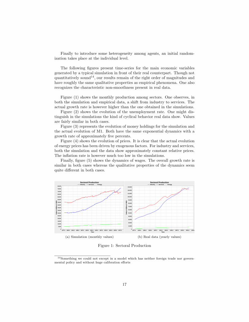
The following figures present time-series for the main economic variablesgenerated by a typical simulation in front of their real counterpart. Though notquantitatively sound14, our results remain of the right order of magnitudes andhave roughly the same qualitative properties as empirical phenomena. One alsorecognizes the characteristic non-smoothness present in real data.

Figure (1) shows the monthly production among sectors. One observes, inboth the simulation and empirical data, a shift from industry to services. Theactual growth rate is however higher than the one obtained in the simulations.

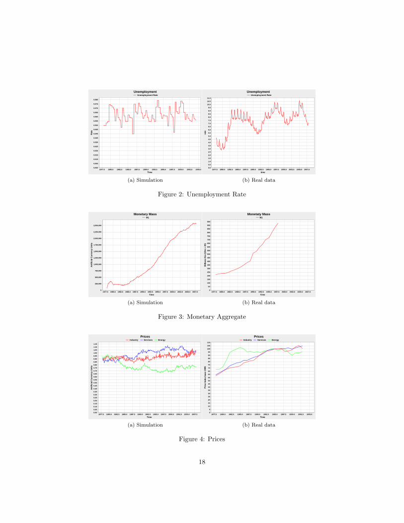
Figure (2) shows the evolution of the unemployment rate. One might dis-tinguish in the simulations the kind of cyclical behavior real data show. Valuesare fairly similar in both cases.

Figure (3) represents the evolution of money holdings for the simulation andthe actual evolution of M1. Both have the same exponential dynamics with agrowth rate of approximately five percents.

Figure (4) shows the evolution of prices. It is clear that the actual evolutionof energy prices has been driven by exogenous factors. For industry and services,both the simulation and the data show approximately constant relative prices.The inflation rate is however much too low in the simulations.

Finally, figure (5) shows the dynamics of wages. The overall growth rate issimilar in both cases whereas the qualitative properties of the dynamics seemquite different in both cases.

Sectoral ProductionIndustry Services Energy

1977.5 1980.0 1982.5 1985.0 1987.5 1990.0 1992.5 1995.0 1997.5 2000.0 2002.5 2005.0 2007.5

Time

0

5,000

10,000

15,000

20,000

25,000

30,000

35,000

40,000

45,000

50,000

55,000

60,000

65,000

70,000

75,000

80,000

Val

ue

in M

illio

n €

200

5

(a) Simulation (monthly values)

Sectoral ProductionIndustry Services Energy

1977.5 1980.0 1982.5 1985.0 1987.5 1990.0 1992.5 1995.0 1997.5 2000.0 2002.5 2005.0

Time

0

10,000

20,000

30,000

40,000

50,000

60,000

70,000

80,000

90,000

100,000

110,000

120,000

130,000

Val

ue

in M

illio

n €

200

5

(b) Real data (yearly values)

Figure 1: Sectoral Production

14Something we could not except in a model which has neither foreign trade nor govern-mental policy and without huge calibration efforts

17

UnemploymentUnemployment Rate

1977.5 1980.0 1982.5 1985.0 1987.5 1990.0 1992.5 1995.0 1997.5 2000.0 2002.5 2005.0

Time

0.000

0.005

0.010

0.015

0.020

0.025

0.030

0.035

0.040

0.045

0.050

0.055

0.060

0.065

0.070

0.075

0.080

Rat

e

(a) Simulation

Unemployment Unemployment Rate

1977.5 1980.0 1982.5 1985.0 1987.5 1990.0 1992.5 1995.0 1997.5 2000.0 2002.5 2005.0 2007.5

time

0.0

0.5

1.0

1.5

2.0

2.5

3.0

3.5

4.0

4.5

5.0

5.5

6.0

6.5

7.0

7.5

8.0

8.5

9.0

9.5

10.0

10.5

11.0

rate

(b) Real data

Figure 2: Unemployment Rate

Monetary MassM1

1977.5 1980.0 1982.5 1985.0 1987.5 1990.0 1992.5 1995.0 1997.5 2000.0 2002.5 2005.0 2007.5

Time

0

250,000

500,000

750,000

1,000,000

1,250,000

1,500,000

1,750,000

2,000,000

2,250,000

2,500,000

Art

ific

ial C

urr

ency

Un

its

(a) Simulation

Monetaty MassM1

1977.5 1980.0 1982.5 1985.0 1987.5 1990.0 1992.5 1995.0 1997.5 2000.0 2002.5 2005.0 2007.5

Time

0

50

100

150

200

250

300

350

400

450

500

550

600

650

700

750

800

850

900

950

Bill

ion

s D

m (

1Dm

= 2

€)

(b) Real data

Figure 3: Monetary Aggregate

PricesIndustry Services Energy

1977.5 1980.0 1982.5 1985.0 1987.5 1990.0 1992.5 1995.0 1997.5 2000.0 2002.5 2005.0 2007.5

Time

0.00

0.05

0.10

0.15

0.20

0.25

0.30

0.35

0.40

0.45

0.50

0.55

0.60

0.65

0.70

0.75

0.80

0.85

0.90

0.95

1.00

1.05

1.10

1.15

Art

ific

ial C

urr

ency

Un

its

(a) Simulation

PricesIndustry Services Energy

1977.5 1980.0 1982.5 1985.0 1987.5 1990.0 1992.5 1995.0 1997.5 2000.0 2002.5 2005.0

Time

0

5

10

15

20

25

30

35

40

45

50

55

60

65

70

75

80

85

90

95

100

105

110

Pri

ce In

dex

bas

e 19

95

(b) Real data

Figure 4: Prices

18

WagesWages

1977.5 1980.0 1982.5 1985.0 1987.5 1990.0 1992.5 1995.0 1997.5 2000.0 2002.5 2005.0 2007.5

Time

0

5

10

15

20

25

30

35

40

45

50

55

60

65

70

Art

ific

ial C

urr

ency

Un

it

(a) Simulation (average wage)

WagesWages

1977.5 1980.0 1982.5 1985.0 1987.5 1990.0 1992.5 1995.0 1997.5 2000.0 2002.5

Time

0.0

0.1

0.2

0.3

0.4

0.5

0.6

0.7

0.8

0.9

1.0

1.1

1.2

1.3

ind

ex b

ase

1990

(b) Real data ( wage Index)

Figure 5: Income

5 Concluding Remarks

The present contribution aims at illustrating a few facts on the use of agent-based models in economics. First, agent-based dynamics could be rigorouslydefined within the seminal framework of analysis of economic systems devisedby Arrow and Debreu in the 1950s (see (Debreu 1959)). They might then helpexplore unknown areas of this map, typically out-of-equilibrium paths. Thishas been achieved by Gintis in (Gintis 2006) and (Gintis 2007) on the issueof equilibrium selection in relatively simple cases. We hope our work mightprove useful to obtain similar insights in more complex frameworks such as(Benhabib and al. 2000).

Second, agent-based dynamics might prove a way to reproduce naively, butaccurately, empirical facts: sound choices for the representation of the behav-ior of micro-economic entities might lead to the emergence of accurate macro-economic properties. The present tentative is in this respect much incomplete,further insight has to be gained on the representation of agent’s decision rules,additional agents (e.g banks) have to be introduced, other phenomena (e.g im-ports and exports, environmental feedbacks) have to be encompassed. We arecurrently working in this direction. However, in this respect, agent-based sim-ulations should not be seen as models of economic reality, but as tools thatmight be used to derive models or to test policy scenarios. The correspondingmathematics might well be different than those of Arrow and Debreu, and moreakin to those of (Peyton-Young 1993) and (Freidlin and Wentzell 1984).

19

References

Arrow, K. (1962) “The economic Implications of Learning by Doing,” TheReview of Economic Studies, Vol. 29, No. 3, pp 155-173.

Benhabib, J. , Meng,Q. and Nishimura,K. (2000) “Indeterminacy under Con-stant Retursn to Scale in Multisector Economies” Econometrica, Vol. 68, No.6 ,pp. 1541-1548

Bilancini, E. and Petri, F. (2008) “The Dynamics of General Equilibrium: AComment on Professor Gintis” Quaderni del dipartimento di economia politica,n. 538, Universita degli studi di siena.

Colander, D. (2006) “Post-Walrasian Macroeconomics: Beyond the DynamicStochastic General Equilibrium Model.” Cambridge University Press, Cam-bridge, U.K., 2006.

Debreu, G (1959) “Theory of Value. An axiomatic analysis of economic equi-librium ”, Cowles Foundation Monograph 17.

Duchin, F. (1998) “Structural Economics: Measuring Change in Technology,Lifestyles and the Environment”, Island Press, Washington, D.C.

Freidlin, M. , and Wentzell,A. (1984) “Random Perturbations of DynamicalSystems” Springer Verlag, New York.

Franklin, S. and Graesser, A. (1997), “Is it an Agent, or just a Program?:A Taxonomy for Autonomous Agents.” Proceedings of the Agent Theories,Architectures, and Languages Workshop, Berlin 1997” Springer Verlag, pp193- 206.

Gintis, H. (2006): “The Emergence of a Price System from Decentralized Bi-lateral Exchange” B. E. Journal of Theoretical Economics, Vol. 6, pp 1302-1322.

Gintis, H. (2007): ”The Dynamics of General Equilibrium.” Economic JournalVol. 117, No. 523, pp. 1280-1309.

Haas, A. and Jaeger, C. (2005) “Agents, Bayes, and Climatic Risks – a modularmodelling approach” Advances in Geosciences, Vol. 4, pp 3–7, 2005.

Jaeger, C. (2005) “A Long-Term Model of the German Economy: lagom d sim”PIK-Report No.102, 2005.

Lebaron, B. and Tesfastion,L. (2008) “Modeling Macroeconomies as Open-Ended Dynamic Systems of Interacting Agents” , American Economic Review,Vol 98, pp. 246-250 .

20

Leijonhufvud, A. (2006) ‘Agent-Based Macro” in Tesfatsion,L. and Judd, K.(eds.), Handbook of Computational Economics, pp 1625-1636.

Luke, S. , Cioffi-Revilla C. , Panait L. , Sullivan,K. and Balan, G (2005)“MASON: A Multi-Agent Simulation Environment´´ , Simulation Vol. 81, pp517-527.

Peyton-Young, H. (1993): “The Evolution of Conventions.” Econometrica, Vol.61, pp 57-84.

Ramsey, PF.P. (1928) ”A Mathematical Theory of Saving”, Economic Journal,Vol. 38, pp 543-59.

Romer,P. (1990) “Endogenous Technological Change.” Journal of PoliticalEconomy. Vol 98, pp 71-102.

Solow, Robert M. (1956) “A Contribution to the Theory of Economic Growth.”Quarterly Journal of Eocnomics Vol. 70, pp 65-94.

Sonnenschein, H. (1973) “ Do Walras’ identity and continuity characterize theclass of community excess demand functions?” Journal of Economic Theory,Vol. 6, pp 345-354

Taylor, J. (1993): “Discretion versus Policy Rules in Practice”, Carnegie-Rochester Conference Series on Public Policy, Vol 39, pp 195-214.

21

ISBN: 978-3-941663-00-8

P.O. Box 600648 14406 Potsdam Germanyinfo@european-climate-forum.net www.european-climate-forum.net

European Climate Forum