Laboratory Evaluation of Corrosion Resistance of Steel ... · DRAFT Laboratory Evaluation of...
161
DRAFT Laboratory Evaluation of Corrosion Resistance of Steel Dowels in Concrete Pavement Prepared for the California Department of Transportation By Mauricio Mancio, Cruz Carlos Jr., Jieying Zhang, John T. Harvey, Paulo J. M. Monteiro, Abdikarim Ali Pavement Research Center Institute of Transportation Studies University of California Berkeley and University of California Davis March, 2005 Revised May 2005
Transcript of Laboratory Evaluation of Corrosion Resistance of Steel ... · DRAFT Laboratory Evaluation of...

DRAFT
Laboratory Evaluation of Corrosion Resistance of Steel Dowels in Concrete Pavement
Prepared for the California Department of Transportation
By
Mauricio Mancio, Cruz Carlos Jr., Jieying Zhang, John T. Harvey, Paulo J. M. Monteiro, Abdikarim Ali
Pavement Research Center Institute of Transportation Studies
University of California Berkeley and University of California Davis
March, 2005 Revised May 2005

ii

iii
TABLE OF CONTENTS
Table of Contents........................................................................................................................... iii
List of Figures ............................................................................................................................... vii
List of Tables ............................................................................................................................... xiii
Executive Summary ...................................................................................................................... xv
Objective of the Study ............................................................................................................. xvi
Dowel Types Evaluated .......................................................................................................... xvii
Test Methods........................................................................................................................... xvii
Experiment Design .................................................................................................................. xix
Phase I................................................................................................................................... xix
Phase II .................................................................................................................................. xx
Phase III ................................................................................................................................ xxi
Conclusions............................................................................................................................. xxii
Phase I Testing..................................................................................................................... xxii
Phase II Laboratory Testing................................................................................................. xxii
Phase III Testing ................................................................................................................. xxiv
Chloride Concentration........................................................................................................ xxv
Recommendations.................................................................................................................. xxvi
1.0 Introduction......................................................................................................................... 1
1.1 Background..................................................................................................................... 2
1.1.1 Corrosion Vulnerability .............................................................................................. 3
1.1.2 Corrosion Prevention .................................................................................................. 5
1.2 Objectives and Scope...................................................................................................... 6
2.0 Experiment Design and Test Procedures ............................................................................ 7

iv
2.1 Phase I: Laboratory Testing ............................................................................................ 8
2.2 Phase II: Laboratory Testing......................................................................................... 11
2.3 Phase III: Evaluation of Field Slabs and Chloride Testing of Cores from Field Slabs 13
2.3.1 Evaluation of Field Slabs .......................................................................................... 13
2.3.2 Chloride Testing of Cores from In-Service Pavements ............................................ 18
2.4 Detection Techniques.................................................................................................... 18
2.5 Holiday Check .............................................................................................................. 21
2.6 Chloride Analyses of Laboratory and Field Cores ....................................................... 22
3.0 Results and Discussion ..................................................................................................... 23
3.1 Phase I Results .............................................................................................................. 23
3.1.1 Half-cell Potential and Linear Polarization Resistance ............................................ 23
3.1.2 Visual Inspection ...................................................................................................... 29
3.2 Phase II Results............................................................................................................. 34
3.2.1 Half-cell Potential and Linear Polarization Resistance ............................................ 34
3.2.2 Statistical Analysis of Results................................................................................... 43
3.2.3 Visual Inspection ...................................................................................................... 45
3.2.4 Microstructural Analysis of Corroded Areas............................................................ 48
3.3 Phase III Results ........................................................................................................... 57
3.3.1 Extracted WSDOT Pavement Slabs.......................................................................... 57
3.4 Analysis of Chloride Contents ...................................................................................... 61
3.4.1 Chloride Analyses from WSDOT Slab Extracted from Interstate 90....................... 61
3.4.2 Chloride Analyses of Cores from WSDOT Pavements in Various Locations ......... 65
3.4.3 Chloride Analyses from Laboratory Samples........................................................... 69

v
4.0 Conclusions and Recommendations ................................................................................. 75
4.1 Phase I Testing Conclusions ......................................................................................... 75
4.2 Phase II Testing Conclusions........................................................................................ 76
4.3 Conclusions from Phase III Testing.............................................................................. 78
4.4 Conclusions from Chloride Analysis ............................................................................ 78
4.5 Recommendations......................................................................................................... 79
5.0 References......................................................................................................................... 81
Appendix A: Detection Techniques............................................................................................ A-1
Half-cell Potential ................................................................................................................... A-1
Linear Polarization Resistance (LPR)..................................................................................... A-3
Physical Inspection ................................................................................................................. A-6
Appendix B: Linear Polarization Results of Individual Specimens ........................................... B-1
Appendix C: Concrete Mix Proportions ..................................................................................... C-1
Appendix D: Chloride Thresholds .............................................................................................. D-1
Appendix E: Half-cell Potentials and Linear Polarization Resistance Laboratory Results .........E-1
Appendix F: Chloride Test Results..............................................................................................F-1
Appendix G: Concrete Technology Laboratories (CTL) Results (Raw Data) ........................... G-1
Appendix H: Characteristics of Microcomposite Steel Used in the Research............................ H-1

vi
vii
LIST OF FIGURES
Figure 1. Schematic representation of steel corrosion sequence in concrete.(6) ............................ 3
Figure 2. Aggressive agents have free access to dowels and are easily dispersed along the length
of the dowel............................................................................................................................. 4
Figure 3. Steel dowel types investigated in Phase I. From top to bottom: carbon steel, stainless
steel clad, carbon steel coated with bendable epoxy, and stainless steel hollow.................... 9
Figure 4. Preparation of dowels before casting in the concrete beams........................................... 9
Figure 5. Half-cell potential test using a high impedance (10 Meg-Ohm) voltmeter, and a
copper/copper sulfate reference cell. .................................................................................... 10
Figure 6. Different types of steel dowels investigated. From left to right: microcomposite steel,
stainless steel hollow, stainless steel clad, non-bendable epoxy-coated dowel (gray coating),
non-flexible epoxy-coated dowel (purple coating), flexible epoxy-coated dowel (green
coating), carbon steel. ........................................................................................................... 12
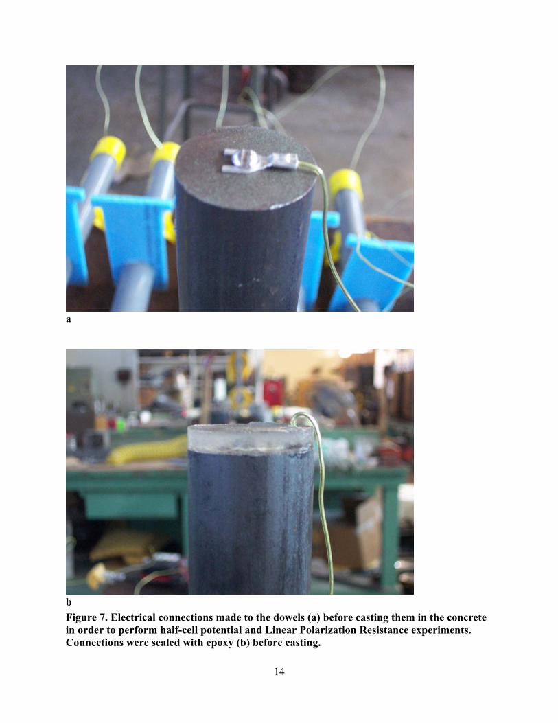
Figure 7. Electrical connections made to the dowels (a) before casting them in the concrete in
order to perform half-cell potential and Linear Polarization Resistance experiments.
Connections were sealed with epoxy (b) before casting....................................................... 14
Figure 8. Electrical connections made to the stainless steel hollow specimens. Connections were
made at the side of the dowel (a) and sealed with epoxy (b) before casting. ....................... 15
Figure 9. Experiment setup to accelerate corrosion using chloride ponding. ............................... 16
Figure 10. Picture of the experimental setup illustrated in Figure 9............................................. 16
Figure 11. WSDOT Slabs at the Pavement Research Center, located at the University of
California Berkeley Richmond Field Station........................................................................ 17
Figure 12. Half-cell potentials of carbon steel bars in Chloride ponding at 40-43ºC................... 24
Figure 13. Half-cell potentials of carbon steel bars in Chloride ponding at 4.4ºC. ...................... 24

viii
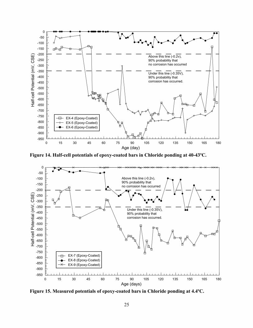
Figure 14. Half-cell potentials of epoxy-coated bars in Chloride ponding at 40-43ºC. ............... 25
Figure 15. Measured potentials of epoxy-coated bars in Chloride ponding at 4.4ºC. .................. 25
Figure 16. Half-cell potentials of stainless hollow steel bars in Chloride ponding at 40-43ºC. ... 26
Figure 17. Half-cell potentials of stainless hollow steel bars in Chloride ponding at 4.4ºC. ....... 26
Figure 18. Half-cell potentials of stainless clad steel bars in Chloride ponding at 40-43ºC. ....... 27
Figure 19. Half-cell potentials of stainless clad steel bars in Chloride ponding at 4.4ºC............. 27
Figure 20. Linear Polarization of the carbon and stainless steels at 40-43ºC............................... 30
Figure 21. Extraction of dowels for visual inspection. ................................................................. 31
Figure 22. Corrosion along the carbon steel bars. ........................................................................ 31
Figure 23. Corrosion on the epoxy-coated bars. ........................................................................... 32
Figure 24. Appearance of stainless steel hollow bars after tests................................................... 33
Figure 25. Appearance of stainless clad bars after tests. .............................................................. 33
Figure 26. Linear Polarization Resistance results for carbon steel dowels................................... 35
Figure 27. Linear Polarization Resistance results for microcomposite steel dowels.................... 36
Figure 28. Linear Polarization Resistance results for stainless steel clad dowels. ....................... 36
Figure 29. Linear Polarization Resistance results for stainless steel hollow dowels.................... 37
Figure 30. Linear Polarization Resistance results for non-flexible, purple epoxy-coated dowels.
............................................................................................................................................... 37
Figure 31. Linear Polarization Resistance results for non-flexible gray epoxy-coated dowels.... 38
Figure 32. Linear Polarization Resistance results for flexible green epoxy-coated dowels. ........ 38
Figure 33. Summary plot showing the variation of potential and current density about the half-
cell potential, for different dowels. ....................................................................................... 40
ix
Figure 34. Detail of the region around the half-cell potential. The greater the slope, the higher the
corrosion resistance............................................................................................................... 40
Figure 35. Comparative column plots showing average results of polarization resistance (Rp) and
corrosion current density (icorr) for non-coated dowels......................................................... 42
Figure 36. Carbon steel dowels. (a) Center region below joint (b) End with electrical connection.
............................................................................................................................................... 46
Figure 37. Microcomposite steel dowels. (a) General view of the center region below joint; (b)
End region............................................................................................................................. 46
Figure 38. Stainless clad dowels. (a) General view of the center region below joint; (b) End
region showing corrosion between the carbon steel core and the stainless steel outer layer.46
Figure 39. Stainless hollow dowels. (a) General view of the center region below joint; (b) End
region showing grouted core................................................................................................. 47
Figure 40. Epoxy-coated dowel (purple). (a) General view of the center region; (b) Corrosion
was verified at the end region, underneath the epoxy seal. .................................................. 47
Figure 41. Epoxy-coated dowel (gray). (a) General view of the center region; (b) Corroded edges
at the end of dowels. ............................................................................................................. 47
Figure 42. Epoxy-coated dowel (green). (a) General view of the center region; (b) Corroded
edges and corrosion underneath coating at the end of dowels.............................................. 48
Figure 43. Corrosion product concentrated in a defective area in the epoxy coating (a); part of the
epoxy coating was removed in order to observe the state of the carbon steel beneath the
coating (b). ............................................................................................................................ 49

x
Figure 44. Carbon steel samples. (a) heavy corrosion along at the dowel surface, magnification =
100×; (b) same region, 200×; (c) different region at the surface, 200×; (d) corrosion at the
bar end, 100×. ....................................................................................................................... 50
Figure 45. Microcomposite steel samples. (a) aspect of corrosion along at the surface, 100×; (b)
same region, 205×; (c) and (d) details of characteristic corrosion sites, 205×. .................... 51
Figure 46. Hollow stainless steel samples: (a) view at the surface, 100×; (b) same region, 300×;
(c) detail of the surface condition, 1000×. The surface appears rough, but no signs of
corrosion damage were observed.......................................................................................... 52
Figure 47. Stainless steel clad samples: (a) aspect of corrosion along the surface, in a region
close to the end of the dowel, 100×; (b) zoom around same region, 200×; (c) details of
corrosion at the surface, interface between sound and corroded area, 2390×; (d) detail of
corrosion at an edge, 2320×. ................................................................................................. 53
Figure 48. Gray-epoxy-coated samples: (a) view of a defect in the coating, with corroded area
inside, 50×; (b) another region, at an edge, where coating is lifted 75×; (c) general view of
the surface, 100×; (d) detail of a pinhole present in image c (see arrow), 1500×. ............... 54
Figure 49. Green-epoxy-coated samples: (a) general view of the surface, 100×; (b) region where
part of the epoxy coating was removed, 100×; (c) condition of the steel underneath the
epoxy, 302×; (d) detail of corroded area and pits present under the coating, 1330×. .......... 55
Figure 50. Purple-epoxy-coated samples: (a) general view of the surface with corrosion products
accumulated in a holiday, 100×; (b) zoom in the same region, 200×; (c) condition of the
steel underneath the epoxy, 200×. ........................................................................................ 56
Figure 51. Linear Polarization Resistance, WSDOT slab, Specimen A....................................... 58
Figure 52. Linear Polarization Resistance, WSDOT slab, Specimen B. ...................................... 58

xi
Figure 53. Linear Polarization Resistance, WSDOT slab, Specimen C. ...................................... 59
Figure 54. Samples extracted from the WSDOT pavement slab for chloride analyses................ 59
Figure 55. View of the interior of a recently made core hole showing corrosion products
underneath the epoxy coating. .............................................................................................. 60
Figure 56. Chloride profile of the slab concrete (Core #1)........................................................... 63
Figure 57. Chloride profile of the slab concrete (Core #2)........................................................... 63
Figure 58. Chloride profile of the grout used for dowel bar retrofit (Core #3). ........................... 64
Figure 59. Chloride profile of the grout around the pavement joint (Core #5). ........................... 64
Figure 60. Chloride profile of the grout around the pavement joint (Core #6). ........................... 65
Figure 61. Chloride profile for SR 5 MP 166.00 (downtown Seattle).......................................... 67
Figure 62. Chloride profile for SR 90 MP 91.324 (Elk Heights). ................................................ 67
Figure 63. Chloride profile for SR 90 MP 61.304 (Price Creek).................................................. 68
Figure 64. Chloride profile for SR 82 MP 10.617 (Military Road).............................................. 68
Figure 65. Chloride profile for SR 82 MP 43.524 (Wapato). ....................................................... 69
Figure 66. Chloride profile on the concrete of a carbon steel specimen....................................... 70
Figure 67. Chloride profile on the concrete of a stainless clad specimen..................................... 71
Figure 68. Chloride profile on the concrete of a stainless hollow specimen. ............................... 71
Figure 69. Chloride profile on the concrete of a flexible (green) epoxy-coated specimen. ......... 72
Figure 70. Chloride profile on the concrete of a non-flexible (purple) epoxy-coated specimen.. 72
Figure 71. Chloride profile on the concrete of a microcomposite steel specimen........................ 73
Figure A1. Apparatus for half-cell potential measurement, described in ASTM C 876.(9)....... A-2
xii
Figure A2. Three-electrode Linear Polarization Resistance method. (a) Measurement of the
open-circuit potential (half-cell potential); (b) Current applied to the counter electrode to
produce a small change in voltage ∆E.(9) .......................................................................... A-4
xiii
LIST OF TABLES
Table 1 Relationship between Half-cell Potential and Corrosion of Steel Embedded in
Concrete (ASTM C 876)....................................................................................................... 19
Table 2 Relationship between Corrosion Current Density and Corrosion Rate(10).............. 20
Table 3 Name Code and Environmental Conditions Used During Phase I ........................... 23
Table 4 Summary Results ...................................................................................................... 41
Table 5 Analysis of Variance (ANOVA) of Half-Cell Potential Results of Non-Coated
Samples ................................................................................................................................. 44
Table 6 Analysis of Variance (ANOVA) of Half-Cell Potential Results of All Samples,
Including Epoxy-Coated Bars............................................................................................... 44
Table 7 Analysis of Variance (ANOVA) of Polarization Resistance (Rp) Results ............... 45
Table 8 Analysis of Variance (ANOVA) of Corrosion Current Density (icorr) Results......... 45
Table 9 Samples Extracted from In-service Pavements for Chloride Analyses (Information
Provided by WSDOT)........................................................................................................... 66
Table A1 Relationship between Half-cell Potential and Corrosion of Steel Embedded in
Concrete (ASTM C 876)..................................................................................................... A-3
Table A2 Relationship between Corrosion Current Density and Corrosion Speed................ A-5

xiv
xv
EXECUTIVE SUMMARY
Dowels are used in jointed concrete pavements to provide load transfer across transverse
joints. Their use reduces vertical deflections that cause faulting and stresses that cause corner and
longitudinal cracking by transferring part of the load to the unloaded slab. However, if corrosion
of the dowels occurs, a number of problems can arise that can compromise the performance of
the pavement and lead to premature failure. These problems include:
• The loss of dowel cross-section, which reduces the capability of the dowel to transfer
loads and restrain vertical movement. The dowel must be tight within the concrete to
effectively minimize slab movement.
• The accumulation of corrosion products, which can potentially restrict the free
expansion and contraction of the slabs, causing lockup and inducing cracks in the
pavement.
Dowel bar corrosion has been investigated in the field and laboratory in the past, which
has lead to the widespread use of epoxy coatings for steel dowels in concrete pavements in place
of bare carbon steel.
Steel reinforcement in sound concrete is protected from corrosion by a passive film
formed due to the high pH (12.5-13.5) of concrete pore solutions. This thin protective film slows
the corrosion reaction rate to very low levels. However, if the passive layer is broken or
dissolves, then the metal reverts to active behavior and rapid corrosion can occur. A conceptual
model proposed by Tuutti represents the process of steel corrosion in reinforced concrete
structures. In Tutti’s model the service life is subdivided into an initiation stage and a
propagation stage.

xvi
The initiation stage is the time necessary for depassiviation of the protective passive layer
as a result of the penetration and concentration of aggressive agents such as carbon dioxide and
chloride ions. For dowels in concrete pavements, the initiation stage is very short because of the
easy access to the dowels by aggressive agents through the joints, and therefore the corrosion
performance of the system depends largely on the properties of the steel dowel being used.
Aggressive agents also potentially access the full length of the dowels because the bond between
the dowels and concrete is designed to be tight, but to have low friction, which probably permits
easier diffusion of the aggressive agents along the dowel than along other reinforcing materials
(rebar). The cyclic horizontal movement of the pavement slabs and the dowel is also likely to
increase the risk of damaging protective coatings such as epoxy.
Most state agencies, including the California Department of Transportation (Caltrans),
seal the joints of concrete pavements in order to minimize the ingress of water and fine debris
into the joint. The effectiveness of this joint sealing practice in preventing aggressive agents
from accessing dowels is unknown. Further, sealing the joint from the surface cannot completely
seal the joint from exposure to water and debris because water and debris can still reach the
dowel from the sides of the joint or from beneath the joint. Aggressive agents can also access the
dowels by penetrating the concrete.
Objective of the Study
The objective of this study was to perform a laboratory investigation of the corrosion
performance of several types of steel dowels embedded in concrete beams. The concrete beams
and dowels were subjected to exposure to concentrated chloride solutions intended to accelerate
corrosion and simulate environmental conditions. The purpose of this investigation was to
develop recommendations for use of different types of dowels for different environmental risk

xvii
conditions. To provide an indication of the aggressiveness of the laboratory conditions relative to
field conditions, a set of field slabs from Washington State was examined, and chloride content
analyses were performed on the concrete beams used in the laboratory studies and on cores taken
from nine locations in Washington State.
Dowel Types Evaluated
The corrosion performance of seven kinds of steel dowel has been evaluated in this study:
bare carbon steel, stainless steel clad, grout-filled hollow stainless steel, microcomposite steel,
carbon steel coated with flexible epoxy (green color code, Designation ASTM A775), and
carbon steel coated with non-flexible epoxies (two types: purple and gray color codes,
Designation ASTM A934).
The stainless clad bars have a core of carbon steel covered by an outer layer
(approximately 5 mm thick) of stainless steel. The ends of the stainless clad dowels do not have
stainless steel cladding, but do have a protective paint coat. Epoxy-coated bars were also epoxy-
coated at the ends. The stainless hollow dowels consisted of a hollow stainless steel cylinder with
a wall thickness of approximately 5 mm, filled with a cementitious grout.
In this study, microcomposite steel refers to microstructurally designed steels with a
ferritic martensitic structure with no carbides, which are anticipated to be more resistant to
corrosion than carbon steel.
Test Methods
Half-cell potential measurements are indicative of the probability of corrosion activity of
the reinforcing steel located beneath the half-cell. The procedure is described by ASTM C 876.
Half-cell potential measurement has been widely used in the field due to its simplicity and
xviii
general agreement that this technique is a good indicator of the existence of active corrosion
along the steel reinforcement in concrete. ASTM C 876 includes a table relating measured
potential and the likelihood of corrosion activity.
The Linear Polarization Resistance (LPR) technique is a well-established method for
determining corrosion rate by using electrolytic test cells. The corrosion rate, expressed as the
corrosion current density is inversely related to the polarization resistance. ASTM G 59 includes
a table with guidelines regarding the relationship between corrosion current density and
corrosion speed.
A major concern with the Linear Polarization Resistance technique is uncertainty about
the area of the steel bar that is affected by the current from the counter electrode. In the present
study, this concern is not justified for the all but the epoxy-coated dowels. It has been assumed
that the area polarized corresponds to that part of the dowel exposed to the NaCl solution inside
the fabricated joint since virtually all the current will flow through the NaCl solution present in
the open joint, which represents a path of very low resistance as compared to concrete. By means
of visual inspection and scanning electron microscopy (SEM), it was found that the corrosion
that occurred in the epoxy-coated dowels was localized and this assumption does not hold.
Therefore, the epoxy-coated dowels could not be evaluated quantitatively using the LPR
technique.
During Phase II of the research, in order to facilitate the identification of corroded areas
in the epoxy-coated dowels and the evaluation of the role of defects in the development of
localized corrosion, the epoxy-coated dowels were checked for holidays (pin-holes, voids,
defects, etc.). This was achieved using a low voltage holiday detector tester before casting the
dowels in concrete beams following ASTM G 62 and CTM 685. This mapping of coating defects
xix
was used to check against locations of corrosion, identified during the visual inspections of
corroded dowels after conditioning. Every epoxy-coated bar examined had one or more defects
on the coating, especially along the edges at the ends. These dowels were shipped from the
manufacturer directly to the laboratory and were subjected to fairly careful handling in the
laboratory.
Chloride analyses were performed on concrete cores extracted from the laboratory beams
from around the dowels in pavement slabs obtained from an early dowel bar retrofit project in
Washington State, and from slab corners of field slabs at six locations in Washington State. The
samples taken from different levels in the cores were tested by the Caltrans chemistry laboratory
or Construction Testing Laboratory in Illinois. Chloride tests were performed following ASTM
C 1152.
Experiment Design
This study was conducted in three phases. Details of the three phases are discussed in the
following sections.
Phase I
Four types of dowels were cast in concrete beams with joints. The four types of dowels
investigated were:
• Carbon steel;
• Stainless steel clad;
• Stainless hollow; and
• Carbon steel coated with flexible epoxy.
xx
The dowels, with diameter 38.1 mm (1.5 in.) and length equal to 460 mm (18 in.), were
cast in concrete beams measuring 150 × 150 × 560 mm (6 × 6 × 22 in.). Electrical connections
were made to the steel bars before casting, expansion end caps were installed on the assembly,
and the dowels were mounted on plastic chairs. In the middle of the concrete beam, a joint was
simulated by using a polystyrene foam spacer, which was removed after 30 days.
The water-to-cement ratio (w/c) of the concrete was 0.42, and the cement:sand:aggregate
ratio was 1:1.84:2.76. Calcium sulfoaluminate cement was used, and the maximum size of the
coarse aggregate was 38 mm (1.5 in.). The specimens were demolded 24 hrs after casting and
cured in a fog room at 23ºC and 100% relative humidity (RH) for 7 days.
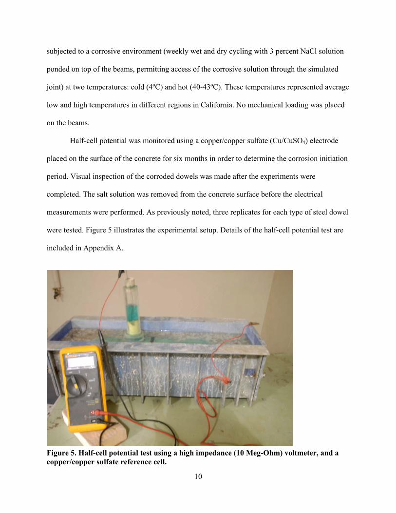
The specimens were then subjected to a corrosive environment (weekly wet and dry
cycling with 3% NaCl solution ponded on top of the beams, permitting access of the corrosive
solution through the simulated joint) at two temperatures: cold (4.4ºC) and hot (40-43ºC). No
mechanical loading was placed on the beams.
Half-cell potential was monitored for six months, and visual inspection of the corroded
dowels was made at the end of testing. Three replicates for each dowel type were tested.
Phase II
Seven types of dowels were cast in concrete beams with joints:
• Carbon steel;
• Microcomposite steel;
• Stainless steel clad;
• Stainless steel hollow;
• Carbon steel coated with flexible epoxy (green color-code); and

xxi
• Carbon steel coated (two types) with non-flexible epoxies (purple and gray color-
codes).
The dimensions of the specimens are the same as those in Phase I, however, a more
permeable concrete was used, with water-to-cement ratio of 0.65 and mix proportions 1:3.0:3.25
(cement:sand:gravel). Type I/II cement was used, and the maximum aggregate size was 12.8 mm
(0.5 in.). The specimens were demolded 24 hours after casting and cured in a fog room at 23ºC
and 100% RH for 28 days.
In the second phase testing, corrosion was accelerated by exposing the samples to cycles
of a 3.5% NaCl solution, at room temperature for a period of 18 months. Half-cell potential tests,
Linear Polarization Resistance curves, visual inspections, chloride content analyses, and
scanning electron microscopic (SEM) investigations were carried out to evaluate the corrosion
performance of the dowels. Four replicates of each type of steel dowel were tested in this phase.
Phase III
Three concrete slabs with two transverse joints were extracted from a dowel bar retrofit
project in Washington. The joints showed loss of load transfer efficiency after 13 years of
service. The slabs and dowels were shipped to Richmond, California and subjected to half-cell
potential tests, Linear Polarization Resistance curves, chloride content tests, and visual
inspections.
This phase of the study also included measurement of chloride contents of concrete cores
taken from transverse joints of field slabs in various climate regions in Washington provided by
the Washington State Department of Transportation (WSDOT), and of cores taken from the
laboratory beam specimens from the Phase II testing, for comparison of the laboratory and field
conditions.

xxii
Conclusions
The following sections present conclusions from the various phases of testing.
Phase I Testing
The following conclusions are drawn from the Phase I testing. Evaluation was made
using half-cell potential tests for corrosion initiation and visual inspection at the completion of
testing.
• Carbon steel dowels present the shortest corrosion initiation period—when chlorides
have direct access to the bar through the joint, the initiation stage can be disregarded
and the corrosion propagation phase begins immediately. Epoxy-coated dowels
exhibited a considerably lengthened initiation period, while the stainless hollow and
stainless clad dowels provided the highest resistance to the onset of corrosion.
• From the visual inspections after 6 months of cyclic ponding, it was observed that the
carbon steel dowels exhibited uniform corrosion along the bar. Epoxy-coated dowels
had localized corrosion at defects—mostly at the ends of the bars where the coating is
most vulnerable to damage. No visible corrosion was observed on either the stainless
steel hollow bars or stainless clad bars.
Phase II Laboratory Testing
The following conclusions are drawn from the Phase II laboratory testing. These
specimens were evaluated for corrosion resistance using half-cell potential tests, Linear
Polarization Resistance curves, visual inspections, chloride analyses, and microscopic
investigations.

xxiii
• In coated specimens, such as the epoxy-coated specimens included in this study,
corrosion is not uniform, but is instead concentrated at localized defective areas (e.g.,
pinholes, voids, etc.). Given that epoxy is an electrical insulator, polarization only
happens at very small locations (defective areas) that cannot be accounted for in the
calculation of the polarization resistance term. Therefore, the epoxy-coated dowels
cannot be quantitatively evaluated with the other dowels and must be evaluated
qualitatively.
• The carbon steel dowels exhibited the lowest values of polarization resistance (Rp)
and therefore have the smallest resistance to charge transfer across the interface.
Carbon steel dowels are therefore expected to have the fastest rate of corrosion
propagation among the types included in this study.
• Microcomposite steel dowels exhibited polarization resistance approximately 35
times larger than carbon steel dowels, while stainless clad and stainless hollow bars
had about 73 times greater polarization resistance. This observation indicates that the
microcomposite steel dowels exhibit much greater resistance to corrosion propagation
than carbon steel dowels, but not as much as the stainless clad and hollow bars.
• Based on corrosion current density results, it was verified that the carbon steel dowels
exhibited very rapid corrosion while microcomposite steel exhibited a moderate level
and stainless steel clad and stainless steel hollow proceeded at low rates of corrosion.
• Visual inspections of the corroded dowels revealed heavy and mostly uniform
corrosion along the carbon steel dowels, light corrosion in the microcomposite steel
dowels, and no visible corrosion in the stainless steel clad and stainless steel hollow
bars. For the epoxy-coated dowels, the visual inspections generally revealed that
xxiv
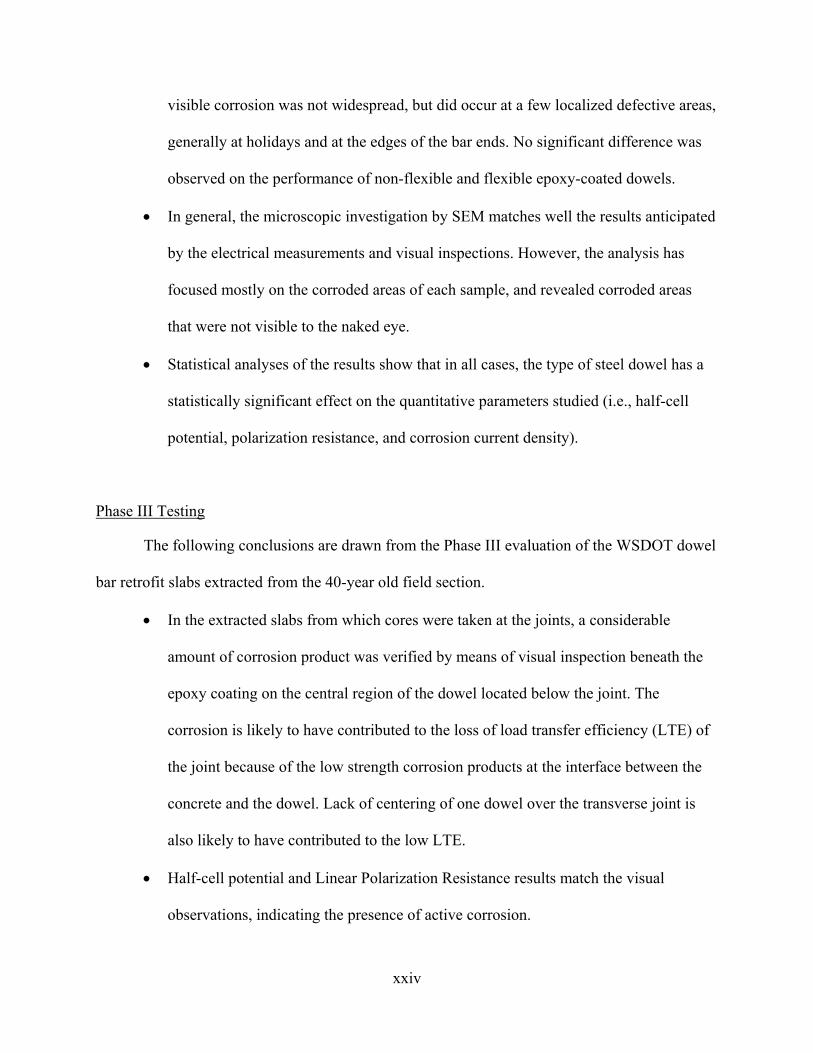
visible corrosion was not widespread, but did occur at a few localized defective areas,
generally at holidays and at the edges of the bar ends. No significant difference was
observed on the performance of non-flexible and flexible epoxy-coated dowels.
• In general, the microscopic investigation by SEM matches well the results anticipated
by the electrical measurements and visual inspections. However, the analysis has
focused mostly on the corroded areas of each sample, and revealed corroded areas
that were not visible to the naked eye.
• Statistical analyses of the results show that in all cases, the type of steel dowel has a
statistically significant effect on the quantitative parameters studied (i.e., half-cell
potential, polarization resistance, and corrosion current density).
Phase III Testing
The following conclusions are drawn from the Phase III evaluation of the WSDOT dowel
bar retrofit slabs extracted from the 40-year old field section.
• In the extracted slabs from which cores were taken at the joints, a considerable
amount of corrosion product was verified by means of visual inspection beneath the
epoxy coating on the central region of the dowel located below the joint. The
corrosion is likely to have contributed to the loss of load transfer efficiency (LTE) of
the joint because of the low strength corrosion products at the interface between the
concrete and the dowel. Lack of centering of one dowel over the transverse joint is
also likely to have contributed to the low LTE.
• Half-cell potential and Linear Polarization Resistance results match the visual
observations, indicating the presence of active corrosion.

xxv
Chloride Concentration
The following conclusions are drawn from the relationship among the concentrations of
chlorides in the laboratory samples, extracted WSDOT field slabs, and cores extracted from slabs
at various locations in Washington State.
• Chloride concentrations close to the pavement joints are significantly higher than in
other regions of the pavement. At the joint, easier access and accumulation of
chlorides leads to higher, localized concentrations.
• When a joint is present, the chloride ions do not diffuse through the concrete (or
grout) from the top; instead, they migrate through the open joint to the dowel.
• In the field cores, it was verified that the chloride threshold for carbon steel was
exceeded in five out of six projects.
• In the laboratory samples, with open joints located above the dowels, the chloride
concentrations are more constant along the depth profile, as compared to field
conditions in which the chlorides have to diffuse through the concrete or migrate
through a narrower joint.
• The use of a 3.5% NaCl solution for laboratory experiments may lead to higher
chloride concentrations than those found in the field specimens, greatly accelerating
the corrosion process compared to the field. As a result of this aggressive
environment, corrosion could be observed in nearly all samples in only 18 months of
exposure.
• Laboratory results can be used to comparatively evaluate the corrosion resistance of
different materials when exposed to the same aggressive environment. However, the
chloride concentration analyses indicate that the actual field conditions and local

xxvi
environment should be taken into account when choosing the appropriate material for
a given project.
Recommendations
The following recommendations are based on the conclusions presented above.
• The presence of corrosion at the bar ends and along the bar from ponding water on
dowels cast in concrete in the laboratory indicates that chlorides can pass all the way
to the bar ends from the joint along the horizontal interface between the dowel and
the concrete, or through the concrete. For this reason it is recommended that uncoated
carbon steel dowels not be used.
• Epoxy dowels present some risk of corrosion, primarily localized at holidays and the
ends. Based on this finding, it is recommended that:
1. Quality control checks to control holidays should be implemented.
2. Bar ends should be coated with epoxy, and care must be taken with epoxy-coated
dowels during shipping, storage, and installation. Corrosion will be exacerbated if
the bar ends are not coated (observed on various Caltrans construction sites) or if
the coated ends are damaged during storage, transport and installation.
• It is recommended that the use of stainless steel clad, hollow stainless steel, or
microcomposite steel dowels be considered for locations with high risk of high
chloride exposure (such as on mountain passes and marine environments), where
exposure to corrosive water is anticipated. The selection of a specific corrosion
resistant dowel should be based on further field investigations and cost differences.

xxvii
• It is recommended that a field study be performed at several mountain pass locations
to measure the chloride content of snow melt after sand/salt application for
comparison with the chloride content of the solution used in the laboratory testing in
Phases I and II and the core results from Phase III. The results of this study should be
used to further refine the risk assessment in these critical locations.

xxviii
1
1.0 INTRODUCTION
The performance of jointed concrete pavements depends to a large extent on adequate
load transfer at the joint. Traffic loads must be effectively transferred across the transverse joints
to minimize differential vertical movement between slabs, and the total movement of each slab.
Minimization of vertical slab movement through the use of dowels has been found to be the most
effective method of slowing the development of faulting, which is a primary cause of roughness
on concrete pavements in California. Effective load transfer at transverse joints also reduces
stresses in the slabs responsible for corner cracking.(1)
Dowels are available in many materials, including stainless steel, epoxy-coated steel, and
fiber reinforced polymer. The most common type is the epoxy-coated steel variety. Dowel bars
provide a mechanical connection between slabs to limit differential vertical movement without
restricting horizontal joint movement. Dowels are usually placed at mid-depth in the slab and
coated with a bond-breaking substance to prevent bonding to the concrete and allow for the
aforementioned horizontal movement.
Corrosion of dowels can compromise the performance of the dowels and of the pavement
in which they are installed and lead to premature failure. In general, concrete seals the steel
dowels from the corrosive effects of weather and environmental exposure, allowing the dowel
bars to function effectively as a long-term reinforcement.(2) However, if corrosion occurs in a
steel-reinforced concrete structure, the expansive steel corrosion products build up tensile stress
in the concrete, often large enough to lead to cracking and deterioration of the structure.(3)
In the case of doweled pavements, the dowel must not have any “play” in the concrete to
achieve maximum load transfer and restriction of vertical movement. The effect of the loss of
cross-section of a dowel due to corrosion introduces “play” and reduces the dowel’s ability to
transfer load and restrain vertical movement. Davids et al. have used finite element analysis to

2
show that a low level of loose fit between the dowel and the concrete can substantially reduce
load transfer efficiency (LTE).(4) Finally, the accumulation of the corrosion products may
restrict the free expansion and contraction of the slabs, causing pavement lock up and potentially
inducing cracks in the pavement.(5)
1.1 Background
The combination of concrete and steel is usually regarded as optimal for both mechanical
performance and durability. Theoretically, this combination should be highly durable, as the
concrete cover provides a chemical and physical protection barrier to the steel, and can
potentially eliminate steel corrosion problems.
Steel reinforcement in sound concrete is protected from corrosion by a passive film
formed due to the high pH (12.5-13.5) of concrete pore solutions. This thin protective film
lowers the corrosion reaction rate to very low levels. However, if the passive layer is broken or
dissolves, then the metal reverts to active behavior and rapid corrosion can occur. In reinforced
concrete, two major factors cause the passive coating to break down:
1. carbonation (reaction with CO2), and
2. the presence of chlorides.
Dowel bar corrosion has been investigated in the field and laboratory in the past, which
has lead to the widespread use of epoxy coatings for steel dowels in concrete pavements in place
of bare carbon steel.

3
1.1.1 Corrosion Vulnerability
In 1982, Tuutti proposed a conceptual model to represent the process of steel corrosion in
reinforced concrete structures. In the model, the service life is subdivided into an initiation stage
and a propagation stage.(6) Figure 1 illustrates this model.
The initiation period is the time necessary for “depassivation” (disruption) of the
protective passive layer. The time to corrosion initiation is determined by how rapidly the
depassivation process occurs as a result of the penetration and concentration of aggressive agents
such as carbon dioxide (CO2) and chloride ions (Cl-).
It is important to note that the initiation stage in Tuutti’s model assumes that the steel
reinforcement or dowels are completely embedded in the concrete, with no direct access by
aggressive agents to the steel except through the intact concrete. However, for dowels in concrete
pavements there is a drastically reduced initiation stage because the access of the aggressive
agents to a dowel bar in a pavement is much easier than to reinforcing steel (rebar) in a structural
concrete element. This is due to the unique functions and design requirements of dowels:
Figure 1. Schematic representation of steel corrosion sequence in concrete.(6)

4
1. The joints through which dowels pass typically allow for free penetration of
aggressive agents such as oxygen, moisture, and de-icing salts to the bar’s surface
(Figure 2). It is recognized that it is not possible to construct and maintain a
completely water- and airtight joint. Water and air can enter the joint from below,
above, and from the sides. Joints are open the widest when temperatures are low,
which in California is the time when most rainfall occurs.
2. Unlike steel placed in concrete for structural reinforcement (rebar), the bond between
the dowels and concrete is designed to be tight, but to have low friction, which likely
permits easier diffusion of the aggressive agents along the dowel than along a rebar.
3. The cyclic horizontal movement between the pavement slabs and the dowel would
increase the risk of damaging protective materials like epoxy-coating.
Thus, aggressive agents such as CO2 and Cl-, plus water and oxygen, have free access to
the steel surface of a dowel, which essentially reduces the time necessary to complete the
initiation stage.
Figure 2. Aggressive agents have free access to dowels and are easily dispersed along the length of the dowel.

5
The beginning of the corrosion process starts at the propagation stage, and the length of
this stage is determined by the rate of corrosion, which is mainly influenced by the moisture
content of the concrete, the temperature, the permeability of the concrete, the chemical
composition of the pore solution, and the thickness of the concrete cover.(6)
1.1.2 Corrosion Prevention
Several methods for reducing the risk of corrosion of steel embedded in concrete exist.
Some are based on the properties of the concrete, and others on the characteristics of the steel
itself.
Over the years, the general approach to improving the durability of reinforced concrete
structures has focused primarily on the improvement of concrete performance. Improvement of
the cracking resistance of the concrete and reduction of concrete permeability, both of which
slow the access of aggressive agents to the passive layer, have produced considerable benefits
and will continue to improve the performance of reinforced concrete structures. However, in the
case of steel doweled pavements, as discussed in the previous section, aggressive agents have
greater access to the steel than in typical steel reinforced concrete and therefore the corrosion
performance of the system depends largely on the properties of the steel dowel being used.
Most state agencies, including the California Department of Transportation (Caltrans),
seal the joints of concrete pavement to minimize the entrance of water and fine debris into the
joint. Sealing is often performed at the time of construction, and joints are often resealed at
intervals in the pavement life. The cost effectiveness of joint sealing is a subject of discussion in
the field of concrete pavements, although most states continue to seal joints. Little research is
available in the literature evaluating the effect of joint sealing on dowel corrosion performance.
Significant research has also improved the corrosion resistance concrete reinforcement, for
6
example, the development of coated steel dowels bars and use of steels with higher corrosion
resistance, as well as several alternatives to regular carbon steel dowels which are now available.
1.2 Objectives and Scope
The main objective of this study was to investigate in the laboratory the corrosion
performance of several types of steel dowels embedded in concrete beams and subjected to
environmental conditions intended to accelerate corrosion by exposure to concentrated chloride
solutions. In this study, seven types of steel dowel were evaluated for their corrosion
performance:
• bare carbon steel,
• stainless steel clad,
• grout-filled hollow stainless steel,
• microcomposite steel,
• carbon steel coated with flexible epoxy (green color code, ASTM Designation A775),
and
• carbon steel coated with non-flexible epoxies (purple and gray color codes, ASTM
Designation A934).
Chapter 2 of this report provides an overview of the experimental work and the
description of the test procedures. Chapter 3 presents the results and discussions of the different
phases of the current study, and Chapter 4 presents the conclusions and recommendations. A
review of the detection techniques used, a brief discussion on chloride thresholds, and detailed
test data and raw data are presented in the appendices.
7
2.0 EXPERIMENT DESIGN AND TEST PROCEDURES
This study included three phases, as follows:
1. Placement of four types of dowels (carbon steel, stainless steel clad, hollow stainless
steel, and epoxy-coated steel dowels) in concrete beams with joints, exposed to a
corrosive environment with chlorides, under two temperature extremes (4ºC and 40-
43ºC). The evaluation included half-cell potential tests over time for the
determination of the corrosion initiation period, and visual inspection at the
completion of testing. Three replicates of each type of dowel were tested.
2. Placement of seven types of dowels cast in concrete beams with joints, exposed to an
accelerated corrosive environment with chlorides. These specimens were evaluated
for corrosion performance using half-cell potential tests, Linear Polarization
Resistance (LPR) experiments, visual inspections, chloride analyses and microscopic
investigations by Scanning Electron Microscope (SEM). In this phase, the in-situ
corrosion rate was measured in order to determine how fast corrosion occurred in the
propagation stage. Four replicates of each type of dowel were tested.
3. Evaluation of three concrete slabs with two transverse joints extracted from a dowel
bar retrofit project in Washington showing loss of load transfer efficiency after 13
years of service. This phase of the study also included measurement of chloride
contents of concrete cores taken from transverse joints of field slabs in various
climate regions in Washington provided by the Washington State Department of
Transportation (WSDOT) for comparison of the laboratory and field conditions.

8
2.1 Phase I: Laboratory Testing
In the first phase, the four types of dowels investigated were:
• Carbon steel. Uncoated and untreated, ASTM A 615.
• Stainless steel hollow. The stainless steel hollow dowels consisted of a hollow type
316 stainless steel cylinder approximately 5 mm thick, filled with a cementitious
grout.
• Stainless steel clad. The stainless clad bars consisted of a core of carbon steel
covered by an outer layer (approximately 5 mm thick) of stainless steel type 316L.
The ends of the dowels did not have stainless steel cladding, but did have a protective
paint coat.
• Carbon steel coated with flexible epoxy. Epoxy-coated dowels with epoxy patch
coating on the ends.
Figure 3 illustrates the dowels used Phase I. All four types of dowels measured 38.1 mm
(1.5 in.) in diameter and 460 mm (18 in.) in length. They were cast in concrete beams measuring
150 × 150 × 560 mm (6 × 6 × 22 in.). As shown in Figure 4, before casting, electrical
connections were made to one end of the steel bars, expansion end caps were placed, and the
dowels were mounted on plastic chairs. In the middle of the concrete beam, a joint was simulated
by using a polystyrene foam spacer, which was carefully removed after 30 days of age.
The water-to-cement ratio (w/c) of the concrete was 0.42, and the cement:sand:aggregate
ratio was 1:1.84:2.76. Calcium sulfoaluminate cement was used, and the maximum size of the
coarse aggregate was 38 mm (1.5 in.). The specimens were demolded 24 hours after casting and
cured at 23ºC and 100 percent relative humidity (RH) for 7 days. These specimens were

9
Figure 3. Steel dowel types investigated in Phase I. From top to bottom: carbon steel, stainless steel clad, carbon steel coated with bendable epoxy, and stainless steel hollow.
Figure 4. Preparation of dowels before casting in the concrete beams.
10
subjected to a corrosive environment (weekly wet and dry cycling with 3 percent NaCl solution
ponded on top of the beams, permitting access of the corrosive solution through the simulated
joint) at two temperatures: cold (4ºC) and hot (40-43ºC). These temperatures represented average
low and high temperatures in different regions in California. No mechanical loading was placed
on the beams.
Half-cell potential was monitored using a copper/copper sulfate (Cu/CuSO4) electrode
placed on the surface of the concrete for six months in order to determine the corrosion initiation
period. Visual inspection of the corroded dowels was made after the experiments were
completed. The salt solution was removed from the concrete surface before the electrical
measurements were performed. As previously noted, three replicates for each type of steel dowel
were tested. Figure 5 illustrates the experimental setup. Details of the half-cell potential test are
included in Appendix A.
Figure 5. Half-cell potential test using a high impedance (10 Meg-Ohm) voltmeter, and a copper/copper sulfate reference cell.

11
2.2 Phase II: Laboratory Testing
Phase II of the testing considered seven different types of dowels:
• Carbon steel. Uncoated and untreated, ASTM A 615.
• Microcomposite steel. Microcomposite steel refers to microstructurally-designed
chromium-containing steels with a ferritic martensitic structure that is virtually
carbide-free. Conventional steels have ferrite-carbide microstructures and, in
corrosive environments, these carbides become cathodic to ferrite and can develop
microgalvanic corrosion cells, which can lead to accelerated corrosion. On the other
hand, microcomposite steels contain ferrite-martensite structures with no carbides,
and thus are anticipated to be more resistant to corrosion (7-9). In this study, the
microcomposite steel specimens presented about 9 percent chromium, according to
information provided by the manufacturer (Appendix H).
• Stainless steel hollow. The stainless steel hollow dowels consisted of a hollow type
316 stainless steel cylinder approximately 5 mm thick, filled with a cementitious
grout.
• Stainless steel clad. The stainless clad bars have a core of carbon steel covered by an
outer layer (approximately 5 mm thick) of stainless steel type 316L. The ends of the
dowels do not have stainless steel cladding, but do have a protective paint coat.
• Carbon steel coated with flexible epoxy (green color code). Epoxy-coated bars
were also epoxy-coated at the ends.
• Carbon steel coated with non-flexible epoxy (two types). Two types were studied:
purple and gray color code epoxy.

12
The dimensions of the specimens are the same as those in Phase I, however a more
permeable concrete was used with a water-to-cement ratio of 0.65 and mix proportions
1:3.0:3.25 (cement:sand:gravel). Type I/II cement was used, and the maximum aggregate size
was 12.8 mm (0.5 in.). The specimens were demolded 24 hours after casting and cured at 23ºC
and 100 percent relative humidity (RH) for 28 days.
In the Phase II testing, corrosion was accelerated by exposing the samples to weekly wet-
and-dry cycles of a 3.5 percent NaCl solution at room temperature for a period of 18 months.
Half-cell potential tests, Linear Polarization Resistance curves, visual inspections, chloride
analyses, and microscopic investigations were carried out to evaluate the corrosion performance
of the dowels. Four replicates of each type of steel dowel were tested in this study. Figures 6
illustrates the different types of dowels used. The in-situ corrosion rate was measured in order to
Figure 6. Different types of steel dowels investigated. From left to right: microcomposite steel, stainless steel hollow, stainless steel clad, non-bendable epoxy-coated dowel (gray coating), non-flexible epoxy-coated dowel (purple coating), flexible epoxy-coated dowel (green coating), carbon steel.
13
permit estimation of the service life of the dowels under the accelerated conditions. Details of the
detection techniques are included in Appendix A. Figures 7 and 8 show the electrical
connections. Figures 9 and 10 demonstrate the experiment setup.
2.3 Phase III: Evaluation of Field Slabs and Chloride Testing of Cores from Field Slabs
In addition to the laboratory experiments described in Section 2.2, further experiments
were performed on concrete pavement slabs obtained from a dowel bar retrofit project from the
Washington Department of Transportation (WSDOT). These slabs were constructed in 1964;
dowel bar retrofit was later performed in 1994. The slabs were extracted from Interstate 90, near
the town of Cle Elum in Washington State, and shipped to the University of California Pavement
Research Center at the Richmond Field Station for testing and evaluation. They were selected
because load transfer efficiencies (LTE) measured using the Falling Weight Deflectometer
(FWD) indicated that the joints were experiencing a decrease in LTE. This was the first WSDOT
dowel bar retrofit project that has shown significant loss of LTE.
According to information provided by WSDOT, until the early 1980’s the approximate
use of rock salt was 120-150 days per year at a typical rate of 180 pounds per mile using a 5:1
ratio (1 scoop of salt to 5 scoops of sand). Each day typically had at least two applications, and
salting typically occurs from mid November to mid April. From the early 1980’s to 1997 or so,
rust inhibitor type deicers/salts have been used. Since 1997, liquid magnesium chloride has been
used at a typical rate of 35 gallons per mile with a range of 15 to 50.
2.3.1 Evaluation of Field Slabs
The slabs used in this study were sawed and sealed during initial construction with a
rubberized joint sealer product called “Seal Target 164.” In 1994, during the dowel bar retrofit,
joints were also sealed with rubberized joint sealant. Figure 11 shows the slabs tested.
14
a
b Figure 7. Electrical connections made to the dowels (a) before casting them in the concrete in order to perform half-cell potential and Linear Polarization Resistance experiments. Connections were sealed with epoxy (b) before casting.

15
a
b Figure 8. Electrical connections made to the stainless steel hollow specimens. Connections were made at the side of the dowel (a) and sealed with epoxy (b) before casting.

16
CROSS - SECTION
SIDE-VIEW
L evel of NaCl solution
Dowel bar
Open-bottom box Open joint
Electrical Connection
3½”
1”
Figure 9. Experiment setup to accelerate corrosion using chloride ponding.
Figure 10. Picture of the experimental setup illustrated in Figure 9.

17
a
b Figure 11. WSDOT Slabs at the Pavement Research Center, located at the University of California Berkeley Richmond Field Station.

18
The location from which these slabs were removed is at an elevation of 543 m. This
location is subject to 568 mm average annual rainfall, 2070 mm average annual snowfall, and 76
average annual freeze-thaw cycles (air temperatures) (16). The slabs were taken from the outside
lane and were subjected to approximately 1 million ESALs annually during their service life.
The dowels are 38 mm in diameter and the concrete slabs 9 in. (228 mm) thick. The dowels were
carbon steel coated with flexible (green) epoxy. After removing the slabs, half-cell potential
tests, Linear Polarization Resistance experiments, chloride analyses and visual inspection work
was performed in order to provide comparison with results obtained in the laboratory under
accelerated conditions. All testing was performed at the University of California, Berkeley
Pavement Research Center.
2.3.2 Chloride Testing of Cores from In-Service Pavements
In addition to the testing performed on the WSDOT slab noted in Section 2.3.1, WSDOT
extracted two cores from near-joint corners of in-service slabs at various locations in
Washington. These cores were tested for chloride content by CTL (Construction Technology
Laboratories, Inc.) for comparison with the laboratory results. (Section 3.4.2 later in this report
describes the locations from which cores were extracted, including years of construction and salt
usage and joint sealing practices.)
2.4 Detection Techniques
Several electrochemical methods have been used to evaluate corrosion activity of steel
reinforcement. The half-cell potential and the Linear Polarization Resistance methods are among
the most commonly used and accepted test methods for in-situ measurements. These tests are
easy to perform in the field, and commercial instruments are readily available. As Carino

19
observes, among the many methods that have been investigated for measuring the in-situ
corrosion rate of steel embedded in concrete, the Linear Polarization Resistance appears to be
gaining most acceptance.(9)
The half-cell potential measurements are indicative of the probability of corrosion
activity of the reinforcing steel located beneath the half-cell, and is described by ASTM C 876.
The setup basically consists of an external electrode (half cell), connecting wires and a high
impedance voltmeter (impedance >10MΩ). A high impedance voltmeter is used so that there is a
very little current through the circuit. Copper/copper sulfate (Cu/CuSO4) electrodes were used
throughout this research.
The half-cell potential measurement has been widely used in the field due to its simplicity
and general agreement among researchers that this technique effectively indicates the existence
of active corrosion along the steel reinforcement in concrete. Table 1 illustrates the relationship
between measured potential and the likelihood of corrosion activity.
Table 1 Relationship between Half-cell Potential and Corrosion of Steel Embedded in Concrete (ASTM C 876)
Half-cell potential (mV)* Corrosion Interpretation > -200 Low probability (10%) of corrosion -200 to -350 Corrosion activity uncertain < -350 High probability (90%) of corrosion * Measurements made with a copper/ copper sulfate electrode.
Thus, the half-cell potential method provides an indication of the likelihood of corrosion
activity at the time of the measurement. However, it does not give any indication of the rate of
corrosion of the steel.

20
On the other hand, the Linear Polarization Resistance (LPR) technique is a well-
established method for determining the rate of corrosion by using electrolytic test cells. The
technique basically involves measuring the change in the open-circuit potential of the electrolytic
cell when an external current is applied to the cell. For a small perturbation about the open-
circuit potential, there is a linear relationship between the change in applied current per unit area
of electrode (∆i) and the change in the measured voltage (∆E). The ratio ∆E/∆i is called the
polarization resistance (Rp). The corrosion rate, expressed as the corrosion current density (i), is
inversely related to the polarization resistance, as indicated by the Stern-Geary relationship i =
B/Rp, where B is a constant (ASTM G 59). Some guidelines have been developed to establish a
relationship between corrosion current density and corrosion rate, as shown in Table 2.(13)
Table 2 Relationship between Corrosion Current Density and Corrosion Rate(13) Corrosion current density, I corr (µA/cm2) Corrosion Rate < 0.1 Negligible 0.1 – 0.5 Low 0.5 – 1.0 Moderate > 1.0 High
A major concern with the LPR method is the uncertainty about the area of the steel bar
that is affected by the current from the counter electrode. Usually, it is assumed that the current
flows in straight lines perpendicular to the bar and the counter electrode, and the affected bar
area is understood to be the bar circumference multiplied by the length of the bar below the
counter electrode, which in fact is not the case, as illustrated in Appendix A. However, in the
laboratory experiments performed in this study (Phases I and II), this concern is not justified,
since virtually all the current will flow through the NaCl solution present in the open joint, which
represents a very low-resistivity path as compared to concrete. As previously stated, the salt

21
solution was removed from the concrete surface in order to perform the electrical measurements,
but the joint remained filled with solution to provide this low-resistivity path for current flow.
Note that the counter electrode (CE) was placed just above the fabricated joint. Thus, it has been
assumed that the area polarized corresponds to that part of the dowel exposed to the NaCl
solution inside the fabricated joint.
In this study, the Linear Polarization Resistance experiments were performed using a
Princeton Applied Research model 263 Potentiostat-Galvanostat. A detailed description of these
detection techniques, along with the explanation of the principles involved, is presented in
Appendix A.
2.5 Holiday Check
During Phase II of this research, in order to facilitate the identification of corroded areas
in the epoxy-coated dowels and the evaluation of the role of defects on the development of
localized corrosion the epoxy-coated dowels were checked for holidays (pin-holes, voids,
defects, etc.). This was done before casting the dowels in the concrete beams using a low voltage
holiday detector tester following ASTM G 62 and CTM 685 (brand Tinker & Rasor, Model M/1
Holiday Detector). This mapping of coating defects was used to check against locations of
corrosion identified during the visual inspections of corroded dowels after conditioning (Section
3.2.2). It is worth mentioning that every single epoxy-coated bar used in Phase II presented one
or more defects on the coating, especially along the edges at the dowel ends. These dowels were
shipped from the manufacturer directly to the laboratory and were subjected to reasonably
careful handling in the laboratory. It would be expected that dowel bars would be subjected to
much rougher handling on a construction site. The holidays found in the mapping were not
caused by being dropped or banged in the laboratory.

22
2.6 Chloride Analyses of Laboratory and Field Cores
Several chloride analyses were performed on concrete cores extracted from the laboratory
beams and from the pavement slabs obtained from WSDOT in order to evaluate the
concentration of chlorides in the region surrounding the steel dowels, particularly in the vicinities
of the open joints. It is believed that over time, chloride ions may build up around the joint area
and close to the dowels, increasing the chloride concentration to considerable levels, perhaps
way above the chloride threshold of the steel being used. The extracted samples were shipped to
the Caltrans chemistry laboratory where the chemical analyses were performed. In addition,
cores from slab corners were obtained from WSDOT pavement at various locations and were
analyzed for chloride content by Construction Technology Laboratories, Inc. Chloride tests are
performed according to ASTM C1152.
23
3.0 RESULTS AND DISCUSSION
The results of the Phase I are presented in Section 3.1 of this report. The results of Phase
II are presented in Section 3.2. The third phase results obtained for the WSDOT slabs from the
dowel bar retrofit project on Interstate 90 and the chloride analyses from the WSDOT cores are
presented in Section 3.3.
3.1 Phase I Results
In the following text and in Figures 12–19, the specimens are identified as RS (“regular
steel,” i.e., carbon steel), SS (stainless steel hollow), EX (epoxy-coated [flexible epoxy, green
code]), and XX (stainless clad bars), as illustrated in Table 3.
Table 3 Name Code and Environmental Conditions Used During Phase I Identification of the specimens
Type of Dowel Hot room (40-43ºC) Cold room (4ºC)
Carbon Steel RS-4, RS-5, RS-6 RS-7, RS-8, RS-9 Stainless Hollow SS-4, SS-5, SS-6 SS-7, SS-8, SS-9 Epoxy-coated EX-4, EX-5, EX-6 EX-7, EX-8, EX-9 Clad XX-4, XX-5, XX-6 XX-1, XX-2, XX-3
3.1.1 Half-cell Potential and Linear Polarization Resistance
Figures 12–19 show the measured half-cell potentials with time for the four types of
dowels investigated in the first phase of this study. As can be observed in Figure 12, for two of
the three replicates of the carbon steels at 40–43ºC, the potentials moved to the active corrosion
region (lower than -350 mV, indicating a 90 percent probability of corrosion as described in
Table 1) after about 75 days. For Specimen RS5, the potentials were more negative than -350
mV from nearly the beginning of the test.

24
0 15 30 45 60 75 90 105 120 135 150 165 180-950
-900
-850
-800-750
-700
-650
-600
-550
-500
-450
-400
-350
-300
-250
-200
-150
-100
-50
0
Age (days)
Hal
f-cel
l Pot
entia
l (m
V, C
SE
)
RS-4 (Carbon Steel)RS-5 (Carbon Steel)RS-6 (Carbon Steel)
Above this line (-0.2v),90% probability thatno corrosion has occurred
Under this line (-0.35V),90% probability thatcorrosion has occurred.
Figure 12. Half-cell potentials of carbon steel bars in Chloride ponding at 40-43ºC.
0 15 30 45 60 75 90 105 120 135 150 165 180-950
-900
-850
-800
-750
-700
-650
-600
-550-500
-450
-400
-350
-300
-250
-200
-150
-100
-50
0
Age (days)
RS-7 (Carbon Steel)RS-8 (Carbon Steel)RS-9 (Carbon Steel)
Hal
f-cel
l Pot
entia
l (m
V, C
SE
)
Above this line (-0.2v),90% probability thatno corrosion has occurred
Under this line (-0.35V),90% probability thatcorrosion has occurred.
Figure 13. Half-cell potentials of carbon steel bars in Chloride ponding at 4.4ºC.
25
0 15 30 45 60 75 90 105 120 135 150 165 180-950
-900
-850
-800
-750
-700
-650
-600
-550-500
-450
-400
-350
-300
-250
-200
-150
-100
-50
0
Age (day)
Above this line (-0.2v),90% probability thatno corrosion has occurred
Under this line (-0.35V),90% probability thatcorrosion has occurred.
EX-4 (Epoxy-Coated)EX-5 (Epoxy-Coated)EX-6 (Epoxy-Coated)
Hal
f-cel
l Pot
entia
l (m
V, C
SE
)
Figure 14. Half-cell potentials of epoxy-coated bars in Chloride ponding at 40-43ºC.
0 15 30 45 60 75 90 105 120 135 150 165 180-950
-900
-850
-800-750
-700
-650
-600
-550
-500
-450
-400
-350
-300
-250
-200
-150
-100
-50
0
Age (days)
EX-7 (Epoxy-Coated)EX-8 (Epoxy-Coated)EX-9 (Epoxy-Coated)
Above this line (-0.2v),90% probability thatno corrosion has occurred
Under this line (-0.35V),90% probability thatcorrosion has occurred.
Hal
f-cel
l Pot
entia
l (m
V, C
SE
)
Figure 15. Measured potentials of epoxy-coated bars in Chloride ponding at 4.4ºC.
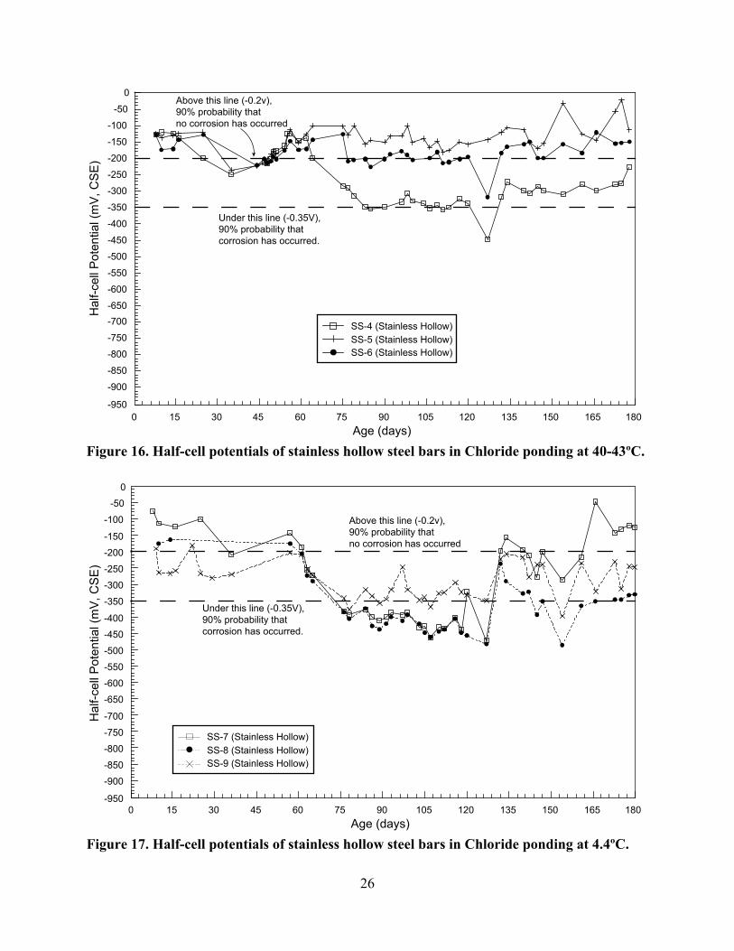
26
0 15 30 45 60 75 90 105 120 135 150 165 180-950
-900
-850
-800
-750
-700-650
-600
-550
-500
-450
-400
-350
-300
-250
-200
-150
-100
-50
0
Age (days)
Hal
f-cel
l Pot
entia
l (m
V, C
SE
)
SS-4 (Stainless Hollow)SS-5 (Stainless Hollow)SS-6 (Stainless Hollow)
Above this line (-0.2v),90% probability thatno corrosion has occurred
Under this line (-0.35V),90% probability thatcorrosion has occurred.
Figure 16. Half-cell potentials of stainless hollow steel bars in Chloride ponding at 40-43ºC.
0 15 30 45 60 75 90 105 120 135 150 165 180-950
-900
-850
-800
-750
-700
-650
-600
-550
-500
-450
-400
-350
-300
-250
-200
-150
-100
-50
0
Age (days)
SS-7 (Stainless Hollow)SS-8 (Stainless Hollow)SS-9 (Stainless Hollow)
Above this line (-0.2v),90% probability thatno corrosion has occurred
Under this line (-0.35V),90% probability thatcorrosion has occurred.
Hal
f-cel
l Pot
entia
l (m
V, C
SE
)
Figure 17. Half-cell potentials of stainless hollow steel bars in Chloride ponding at 4.4ºC.

27
0 15 30 45 60 75 90 105 120 135 150 165 180-950
-900-850-800
-750-700-650
-600-550
-500-450-400
-350-300-250
-200-150-100
-500
Age (days)
Above this line (-0.2v),90% probability thatno corrosion has occurred
Under this line (-0.35V),90% probability thatcorrosion has occurred.
Hal
f-cel
l Pot
entia
l (m
V, C
SE
)
XX-4 (Stainless Clad)XX-5 (Stainless Clad)XX-6 (Stainless Clad)
Figure 18. Half-cell potentials of stainless clad steel bars in Chloride ponding at 40-43ºC.
0 15 30 45 60 75 90 105 120 135 150 165 180-950
-900
-850
-800
-750
-700
-650
-600
-550
-500
-450
-400
-350
-300
-250
-200
-150
-100
-500
XX-1 (Stainless Clad)XX-2 (Stainless Clad)XX-3 (Stainless Clad)
Above this line (-0.2v),90% probability thatno corrosion has occurred
Under this line (-0.35V),90% probability thatcorrosion has occurred.
Hal
f-cel
l Pot
entia
l (m
V, C
SE
)
Age (days) Figure 19. Half-cell potentials of stainless clad steel bars in Chloride ponding at 4.4ºC.

28
As discussed in Section 1.1.1, compared to reinforcing steel in concrete structures in
which the steel is completely encased in concrete, the initiation period may be greatly reduced in
the case of steel dowels due to the easier access of aggressive agents to the bars.
At 4.4ºC (Figure 13), potentials moved to the active corrosion zone after about 30 days
for RS7 and RS9, and not until 75 days for RS8. It is interesting to notice that for some
specimens, corrosion was initiated earlier for carbon steels in the 4.4ºC room than those in 40-
43ºC. The reason may be the difference in oxygen availability at different temperatures. The
higher the temperature, the lower is the oxygen solubility in water. For instance, oxygen
solubility in saltwater is about 11.7 mg/L at 4ºC, and the value drops to 6.5 mg/L at 30ºC.
It is important to mention that the polystyrene foam sheet used to create the joints was
removed after 30 days of age. After the polystyrene sheet was removed, corrosion was
immediate for the carbon steel in the 4.4ºC room, which indicates that the pavement joint is the
dominant access of chloride, oxygen, and water to the dowel surface. This suggests that joint
sealing may potentially reduce the likelihood of, or retard the rate of corrosion of dowels by
limiting access of corrosive solutions. However, joints are typically only sealed at the surface
and corrosive solutions may be able to enter the joint from the sides and bottom of the joint in
addition to the surface.
For the epoxy-coated steel bars at high temperatures (40–43ºC) (see Figures 14 and 15),
the measured potentials for Specimens EX4 and EX5 experienced an abrupt decrease at around
40 days to approximately -650mV in the high-corrosion risk region. Specimen EX6, on the other
hand, measured zero and stayed in the inactive region throughout the test.
For cold temperature specimens (4ºC), the measured potential of Specimen EX9
remained at zero throughout the test, possibly indicating absence of defects in its epoxy coating,

29
or perhaps some problem with the electrical connection at the dowel. The potentials of Specimen
EX7 oscillated within the intermediate corrosion risk (uncertain) range, while Specimen EX8
entered the high-corrosion risk region (< -350mV) at around 70 days. Note that, in Phase I of the
study, the epoxy coating was not checked for defects before casting. This procedure was adopted
in the second phase, as described in Section 2.2.
Both stainless hollow and stainless clad dowels (Figures 16 to 19) generally had
measured potentials above the -350 mV line at both test temperatures, indicating low probability
of corrosion.
In the first phase, emphasis was placed on the determination of the initiation period based
on the measurement of half-cell potentials over time. However, a Linear Polarization Resistance
test to evaluate corrosion rate was also performed on the carbon and stainless steel dowels.
Figure 20 shows the results obtained (specimens were stored at 40–43ºC). The slope of a
polarized potential and corresponding current supply curve is the polarization resistance, Rp. Its
value is inversely proportional to the corrosion rate (i) indicated in Stern-Geary relationship i =
B/Rp, where B is a constant with the value from 25 mV to 56 mV. The corrosion rate of carbon
steel can be 10 times as high as that of the stainless steel. Note that the corrosion rate of RS4 was
low while its half-cell potential was located in the active corrosion region (<-350mV), indicating
that the half-cell potential measurement is not a quantitative method. Results from the other two
specimens (RS5 and RS6) matched the half-cell potential measurements well.
3.1.2 Visual Inspection
At the end of six months, the concrete beams were broken open and the dowels were
retrieved and inspected. Figure 21 shows one of the concrete beams at the moment the dowel
was being retrieved.

30
-0.10 -0.05 0.00 0.05 0.10
-80
-60
-40
-20
0
20
40
60
80
Current (mA)
SS4 (Stainless Hollow)
SS5 (Stainless Hollow)
SS6 (Stainless Hollow)RS4 (Carbon Steel)RS5 (Carbon Steel)
RS6 (Carbon Steel)
Hotroom Age: 130 DaysP
oten
tial (
mV
)
Figure 20. Linear Polarization of the carbon and stainless steels at 40-43ºC.
For the carbon steels exposed to Chloride ponding, corrosion products were distributed
along the length and perimeter of the bars for both the cold and hot conditions, as shown in
Figure 22. The epoxy-coated bars had localized corrosion mostly at the ends of the bars where
the coating is the most vulnerable to damage. All the epoxy-coated bars exposed to Chloride
ponding, except EX9, were corroded at the ends, as shown in Figure 23. The results matched the
half-cell potential in the sense that once corrosion occurred and the coating was lifted, the
measured potential was not zero anymore. No visible corrosion was found on either stainless
steel hollow bars or stainless clad bars, as can be observed in Figures 24 and 25.
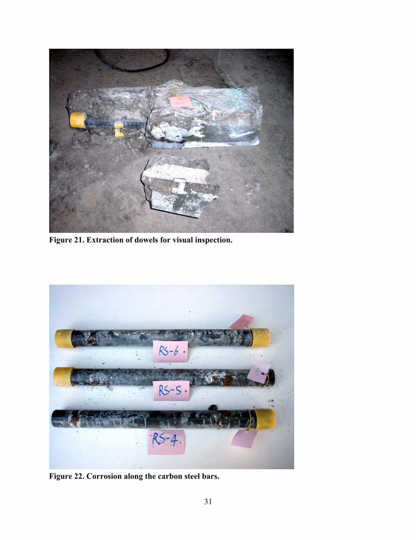
31
Figure 21. Extraction of dowels for visual inspection.
Figure 22. Corrosion along the carbon steel bars.

32
Figure 23. Corrosion on the epoxy-coated bars.

33
Figure 24. Appearance of stainless steel hollow bars after tests.
Figure 25. Appearance of stainless clad bars after tests.
34
3.2 Phase II Results
This section presents the results obtained in the second phase of the research, in which
half-cell potential tests, Linear Polarization Resistance curves, visual inspections, chloride
analyses and microscopic investigation were obtained at room temperature on the seven types of
steel dowels investigated [carbon steel, microcomposite steel, stainless hollow, stainless clad,
carbon steel coated with flexible epoxy (green colored), and carbon steel coated with non-
flexible epoxies (purple and gray colored)].
3.2.1 Half-cell Potential and Linear Polarization Resistance
In this section, individual graphs present the Linear Polarization Resistance results for
each type of dowel investigated. The plots present the average results of four replicates
normalized with respect to the half-cell value. Current density (µA/cm2) and potential (mV) are
given as variations from the values obtained at equilibrium, half-cell potential. Normalizing the
data facilitates comparison among the different samples. Non-normalized results for each type of
steel dowel are presented in Appendix B.
As described in Section 2.1, the slope of the curves (∆E/∆i) provides the value of the
polarization resistance, Rp. Notice that the greater the slope, the more difficult the charge
transfer across the metal/electrolyte interface, and therefore the corrosion current density is lower
and, consequently, the corrosion reaction rate is slower.
Figures 26 to 29 present the Linear Polarization Resistance plots for the carbon steel,
microcomposite, hollow stainless steel, and stainless steel clad bars, respectively. It can be seen
that for the same variation in potential, carbon steel bars exhibit a much larger variation in the
corrosion current density compared to the other materials. Consequently, the carbon steel

35
samples will exhibit a smaller slope, smaller polarization resistance, and larger corrosion rate,
followed by microcomposite steel, stainless steel clad, and stainless steel hollow, respectively.
Figures 30-32 present Linear Polarization Resistance plots for the epoxy-coated bars,
respectively non-flexible (purple and gray) and flexible (green) epoxy coatings. Note that the
results obtained for the epoxy-coated bars are not to be interpreted quantitatively. In coated
specimens, corrosion is not uniform. Rather, it is concentrated at localized defective areas (such
as pinholes, voids, etc.). Given that epoxy is an electrical insulator, polarization only occurs at
these defective areas which cannot be accounted for in the calculation of the polarization
resistance term. As mentioned in Section 2, it has been assumed that the polarized area
corresponds to the surface of the dowels exposed to the NaCl solution inside the fabricated
joints. Note that if the polarized area decreases in size, the corrosion current density (given in
y = 2.9143x - 0.2403R2 = 0.9902
-30
-20
-10
0
10
20
30
-10 -8 -6 -4 -2 0 2 4 6 8
Current Density (µA/cm2)
Pote
ntia
l Var
iatio
n (m
V)
Figure 26. Linear Polarization Resistance results for carbon steel dowels.

36
y = 41.802x + 2.3608R2 = 0.9515
-30
-20
-10
0
10
20
30
-1.0 -0.8 -0.6 -0.4 -0.2 0.0 0.2 0.4 0.6
Current Density (µA/cm2)
Pote
ntia
l Var
iatio
n (m
V)
Figure 27. Linear Polarization Resistance results for microcomposite steel dowels.
y = 279.31x + 4.6152R2 = 0.9204
-30
-20
-10
0
10
20
30
-0.15 -0.12 -0.09 -0.06 -0.03 0.00 0.03 0.06
Current Density (µA/cm2)
Pote
ntia
l Var
iatio
n (m
V)
Figure 28. Linear Polarization Resistance results for stainless steel clad dowels.

37
y = 258.13x + 1.6974R2 = 0.9312
-30
-20
-10
0
10
20
30
-0.15 -0.12 -0.09 -0.06 -0.03 0.00 0.03 0.06 0.09
Current Density (µA/cm2)
Pote
ntia
l Var
iatio
n (m
V)
Figure 29. Linear Polarization Resistance results for stainless steel hollow dowels.
y = 91.692x - 0.2301R2 = 0.9988
-30
-20
-10
0
10
20
30
-0.30 -0.25 -0.20 -0.15 -0.10 -0.05 0.00 0.05 0.10 0.15 0.20 0.25
Current Density (µA/cm2)
Pote
ntia
l Var
iatio
n (m
V)
Figure 30. Linear Polarization Resistance results for non-flexible, purple epoxy-coated dowels.

38
y = 366.55x + 0.2249R2 = 0.9657
-30
-20
-10
0
10
20
30
-0.10 -0.08 -0.06 -0.04 -0.02 0.00 0.02 0.04 0.06 0.08
Current Density (µA/cm2)
Pote
ntia
l Var
iatio
n (m
V)
Figure 31. Linear Polarization Resistance results for non-flexible gray epoxy-coated dowels.
y = 409.59x + 2.9279R2 = 0.9348
-30
-20
-10
0
10
20
30
-0.09 -0.07 -0.05 -0.03 -0.01 0.01 0.03 0.05 0.07
Current Density (µA/cm2)
Pote
ntia
l Var
iatio
n (m
V)
Figure 32. Linear Polarization Resistance results for flexible green epoxy-coated dowels.

39
µA/cm2) will increase. The surface area used in the current density calculations was 7.18 cm2,
which corresponds to the dowel bar circumference (119.69mm) multiplied by the thickness of
the joint (6mm). The microcomposite steel dowels had smaller diameter (1.25 in. or 31.75mm),
and the polarized area was thus 5.98 cm2.
The fact that electrical contact can be made between the reference electrode
(copper/copper sulfate) and the working electrode (steel dowel), and that a half-cell potential can
be measured for epoxy-coated bars, indicates the presence of defects in the coating. The Linear
Polarization Resistance results may indicate the presence of corrosion in the defective areas, but
an evaluation of the extent of corrosion must rely on the visual inspections and microscopic
investigations.
Figures 33 and 34 present a comparison of the Linear Polarization Resistance results of
various dowels. It can be easily seen that the carbon steel specimens performed much worse than
the other dowels tested. On the other hand, it can be observed that the stainless steel hollow bars
exhibited the best performance, followed by stainless steel clad and microcomposite steel
dowels. Table 4 summarizes the individual results obtained for each sample including half-cell
potential, polarization resistance (Rp) and corrosion current density (icorr). (Plots with
calculations are presented in Appendix B.) The criteria used to interpret the results presented in
Table 4 are per ASTM C 876 and ASTM G 59 and are presented in Tables 1 and 2, respectively.
Figure 35 presents a comparative summary of Linear Polarization Resistance and current density
results.
Regarding the half-cell potential values, note that the stainless steel hollow and stainless
steel clad specimens are, on average, located in the uncertain corrosion region, while all the other
samples are in the active corrosion region (refer to Table 1).

40
-25.0
-20.0
-15.0
-10.0
-5.0
0.0
5.0
10.0
15.0
20.0
25.0
-9.0 -8.0 -7.0 -6.0 -5.0 -4.0 -3.0 -2.0 -1.0 0.0 1.0 2.0 3.0 4.0 5.0 6.0 7.0 8.0
Current Density (µA/cm2)
Pote
ntia
l Var
iatio
n (m
V)
Carbon Steel
Microcomposite Steel
Stainless Steel Clad
Stainless Steel Hollow
Figure 33. Summary plot showing the variation of potential and current density about the half-cell potential, for different dowels.
-25.0
-20.0
-15.0
-10.0
-5.0
0.0
5.0
10.0
15.0
20.0
25.0
-1.5 -1.3 -1.1 -0.9 -0.7 -0.5 -0.3 -0.1 0.1 0.3 0.5 0.7 0.9 1.1 1.3 1.5
Current Density (µA/cm2)
Pote
ntia
l Var
iatio
n (m
V)
Carbon Steel
Microcomposite Steel
Stainless Steel Clad
Stainless Steel Hollow
Figure 34. Detail of the region around the half-cell potential. The greater the slope, the higher the corrosion resistance.
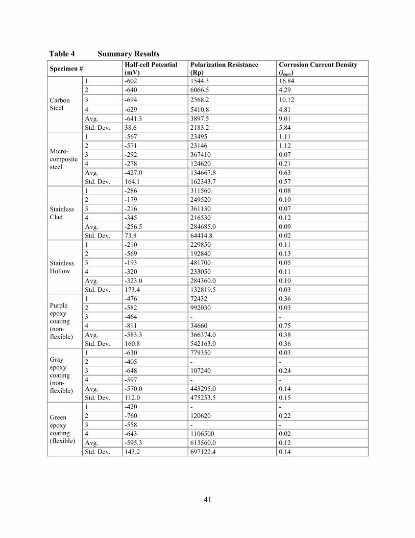
41
Table 4 Summary Results
Specimen # Half-cell Potential (mV)
Polarization Resistance (Rp)
Corrosion Current Density (icorr)
1 -602 1544.3 16.84 2 -640 6066.5 4.29 3 -694 2568.2 10.12 4 -629 5410.8 4.81 Avg. -641.3 3897.5 9.01
Carbon Steel
Std. Dev. 38.6 2183.2 5.84 1 -567 23495 1.11 2 -571 23146 1.12 3 -292 367410 0.07 4 -278 124620 0.21 Avg. -427.0 134667.8 0.63
Micro-composite steel
Std. Dev. 164.1 162343.7 0.57 1 -286 311560 0.08 2 -179 249520 0.10 3 -216 361130 0.07 4 -345 216530 0.12 Avg. -256.5 284685.0 0.09
Stainless Clad
Std. Dev. 73.8 64414.8 0.02 1 -210 229850 0.11 2 -569 192840 0.13 3 -193 481700 0.05 4 -320 233050 0.11 Avg. -323.0 284360.0 0.10
Stainless Hollow
Std. Dev. 173.4 132819.5 0.03 1 -476 72432 0.36 2 -582 992030 0.03 3 -464 - - 4 -811 34660 0.75 Avg. -583.3 366374.0 0.38
Purple epoxy coating (non-flexible)
Std. Dev. 160.8 542163.0 0.36 1 -630 779350 0.03 2 -405 - - 3 -648 107240 0.24 4 -597 - - Avg. -570.0 443295.0 0.14
Gray epoxy coating (non-flexible)
Std. Dev. 112.0 475253.5 0.15 1 -420 - - 2 -760 120620 0.22 3 -558 - - 4 -643 1106500 0.02 Avg. -595.3 613560.0 0.12
Green epoxy coating (flexible)
Std. Dev. 143.2 697122.4 0.14

42
3897.45
134667.75
0
50000
100000
150000
200000
Carbon Steel Microcomposite Steel Stainless Steel Clad Stainless Steel Hollow
Dowel Type
Line
ar P
olar
izat
ion
Res
ista
nce
Figure 35a.
0.6
0.1 0.1
0.0000
1.0000
2.0000
3.0000
4.0000
Carbon Steel Microcomposite Steel Stainless Steel Clad Stainless Steel Hollow
Dowel Type
Cur
rent
Den
sity
(ico
rr)
Figure 35b. Figure 35. Comparative column plots showing average results of polarization resistance (Rp) and corrosion current density (icorr) for non-coated dowels.

43
With respect to the average corrosion current densities, one can observe that the carbon
steel dowels exhibit very rapid corrosion while microcomposite steel exhibits a moderate level of
corrosion. Stainless steel clad and stainless steel hollow dowels proceed at a low corrosion rate
(refer to Tables 1 and 2 for criteria used). Individual results show that two out of four
microcomposite samples were in the “uncertain” corrosion region (as per half-cell potential
results), and presented low corrosion rate.
The average values presented for the epoxy-coated bars also indicate a low corrosion rate
and, in fact, visual inspection (Section 3.2.3) revealed no major signs of corrosion for these
dowels, except at a few localized defective areas. However, LPR results for epoxy-coated bars
cannot be interpreted quantitatively. As is further discussed in Section 3.2.4 (microstuctural
analysis), localized corrosion was identified at defects in the coating. Additional corrosion was
also observed under the coating.
3.2.2 Statistical Analysis of Results
The Analysis of Variance (ANOVA) model was used to evaluate the results obtained and
to verify if there is a statistically significant effect of the type of steel dowel on the parameters
investigated. Basically, the Analysis of Variance table takes into account the effect of the
factor(s) being studied and the variability of the experiments (i.e., the experimental error) to
determine whether the results obtained are statistically significant at a confidence interval of 95
percent. The analysis is based on the so-called “F-test,” in which the calculated value of the
parameter F (“Fcalc”) is compared to the critical value “Fcrit” If Fcalc > Fcrit., it is said that the
effect is statistically significant.
In the case of the research presented herein, the factor or independent variable being
analyzed is the type of steel dowel, and the dependent variable is the experimental result
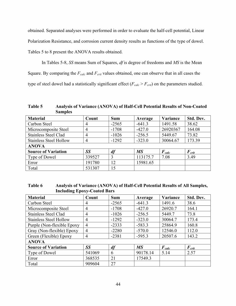
44
obtained. Separated analyses were performed in order to evaluate the half-cell potential, Linear
Polarization Resistance, and corrosion current density results as functions of the type of dowel.
Tables 5 to 8 present the ANOVA results obtained.
In Tables 5-8, SS means Sum of Squares, df is degree of freedoms and MS is the Mean
Square. By comparing the Fcalc and Fcrit values obtained, one can observe that in all cases the
type of steel dowel had a statistically significant effect (Fcalc > Fcrit) on the parameters studied.
Table 5 Analysis of Variance (ANOVA) of Half-Cell Potential Results of Non-Coated Samples
Material Count Sum Average Variance Std. Dev. Carbon Steel 4 -2565 -641.3 1491.58 38.62 Microcomposite Steel 4 -1708 -427.0 26920367 164.08 Stainless Steel Clad 4 -1026 -256.5 5449.67 73.82 Stainless Steel Hollow 4 -1292 -323.0 30064.67 173.39 ANOVA Source of Variation SS df MS Fcalc Fcrit Type of Dowel 339527 3 113175.7 7.08 3.49 Error 191780 12 15981.65 Total 531307 15
Table 6 Analysis of Variance (ANOVA) of Half-Cell Potential Results of All Samples, Including Epoxy-Coated Bars
Material Count Sum Average Variance Std. Dev. Carbon Steel 4 -2565 -641.3 1491.6 38.6 Microcomposite Steel 4 -1708 -427.0 26920.7 164.1 Stainless Steel Clad 4 -1026 -256.5 5449.7 73.8 Stainless Steel Hollow 4 -1292 -323.0 30064.7 173.4 Purple (Non-flexible Epoxy 4 -2333 -583.3 25864.9 160.8 Gray (Non-flexible) Epoxy 4 -2280 -570.0 12546.0 112.0 Green (Flexible) Epoxy 4 -2381 -595.3 20507.6 143.2 ANOVA Source of Variation SS df MS Fcalc Fcrit Type of Dowel 541069 6 90178.14 5.14 2.57 Error 368535 21 17549.3 Total 909604 27

45
Table 7 Analysis of Variance (ANOVA) of Polarization Resistance (Rp) Results Material Count Sum Average Variance Std. Dev. Carbon Steel 4 15589.8 3897.45 4766409 2183.2 Microcomposite Steel 4 538671 134667.8 2.64E+10 162343.7 Stainless Steel Clad 4 1138740 284685 4.15E+09 64414.8 Stainless Steel Hollow 4 1137440 284360 1.76E+10 132819.5 ANOVA Source of Variation SS df MS Fcalc Fcrit Type of Dowel 2E+11 3 7.32E+10 6.08 3.49 Error 1!+11 12 1.2E+10 Total 4E+11 15 Table 8 Analysis of Variance (ANOVA) of Corrosion Current Density (icorr) Results Material Count Sum Average Variance Std. Dev. Carbon Steel 4 36.051 9.0127 34.162 5.845 Microcomposite Steel 4 2.509 0.6273 0.320 0.566 Stainless Steel Clad 4 0.380 0.0949 0.000 0.021 Stainless Steel Hollow 4 0.413 0.1034 0.001 0.035 ANOVA Source of Variation SS df MS Fcalc Fcrit Type of Dowel 229.78 3 76.59247 8.88 3.49 Error 103.45 12 8.621028 Total 333.23 15
3.2.3 Visual Inspection
After the electrical experiments were finished, one beam of each dowel type was cored at
the joint in order to analyze the concentration of chlorides in the concrete surrounding the
dowels. The remainder of the specimens were cut open and broken to retrieve the dowels for
visual inspection of the corroded areas. At this moment, specimens were selected for the
microstructural SEM (Scanning Electron Microscope) analyses presented in Section 3.2.3.
Figures 36 through 42 illustrate the general appearance of the inspected dowels. In
general, carbon steel dowels exhibited generalized corrosion along the bars. Microcomposite
steel dowels showed significantly less corrosion (as compared to carbon steel specimens).
Stainless clad dowels had no visible corroded areas along the bars (corrosion was verified at the

46
a B Figure 36. Carbon steel dowels. (a) Center region below joint (b) End with electrical connection.
A b Figure 37. Microcomposite steel dowels. (a) General view of the center region below joint; (b) End region.
A b Figure 38. Stainless clad dowels. (a) General view of the center region below joint; (b) End region showing corrosion between the carbon steel core and the stainless steel outer layer.

47
A b Figure 39. Stainless hollow dowels. (a) General view of the center region below joint; (b) End region showing grouted core.
A b Figure 40. Epoxy-coated dowel (purple). (a) General view of the center region; (b) Corrosion was verified at the end region, underneath the epoxy seal.
A b Figure 41. Epoxy-coated dowel (gray). (a) General view of the center region; (b) Corroded edges at the end of dowels.

48
A b Figure 42. Epoxy-coated dowel (green). (a) General view of the center region; (b) Corroded edges and corrosion underneath coating at the end of dowels.
ends between the carbon steel core and outer stainless steel layer). Stainless hollow dowels
showed basically no visible corrosion. Localized corrosion was verified in the defective regions
on the epoxy-coated dowels, but no major signs of corrosion could be observed visually.
As seen in Figures 36–42, the carbon steel samples were heavily corroded. The
microcomposite steel dowels exhibited less corrosion. The stainless steel clad and stainless steel
hollow dowels showed essentially no visible signs of corrosion. Defects were observed in the
epoxy-coated bars and, as expected, localized corrosion in the defective regions was verified.
3.2.4 Microstructural Analysis of Corroded Areas
The microstructural investigation was performed with a digital Leo 430 Scanning
Electron Microscope (SEM) using secondary electrons. The SEM imaging consists of
bombarding the sample with an electron beam with sufficient energy to excite and eject
secondary electrons, which are detected and recorded using a CCD camera.
In this study, samples of each corroded dowel type were collected during the visual
inspection and then analyzed by SEM.

49
In the SEM microstructural analysis, preference was given to the inspection of the
corroded areas in each sample (e.g., Figure 43a). In addition, selected regions such as the one
illustrated in Figure 43b were also investigated. Figures 44 to 50 present characteristic SEM
pictures for each material investigated.
In general, the severity of the corrosion observed with the electron microscope matches
the results anticipated by the electrical measurements and visual inspections. However, one
should keep in mind that the microstructural investigation focused mostly on the corroded areas
of each sample, and does not represent the general state of the dowel bars. The stainless steel
clad dowels, for example, exhibited excellent performance on the corrosion rate measurements,
and no corrosion was identified by visual inspection, however, relatively severe localized
corrosion was observed at the ends of the dowels close to the interface with carbon steel (see
Figures 38b and 47).
a b Figure 43. Corrosion product concentrated in a defective area in the epoxy coating (a); part of the epoxy coating was removed in order to observe the state of the carbon steel beneath the coating (b).

50
a b
c d Figure 44. Carbon steel samples. (a) heavy corrosion along at the dowel surface, magnification = 100×; (b) same region, 200×; (c) different region at the surface, 200×; (d) corrosion at the bar end, 100×.

51
a b
c d Figure 45. Microcomposite steel samples. (a) aspect of corrosion along at the surface, 100×; (b) same region, 205×; (c) and (d) details of characteristic corrosion sites, 205×.

52
a b
c
Figure 46. Hollow stainless steel samples: (a) view at the surface, 100×; (b) same region, 300×; (c) detail of the surface condition, 1000×. The surface appears rough, but no signs of corrosion damage were observed.

53
a b
c d Figure 47. Stainless steel clad samples: (a) aspect of corrosion along the surface, in a region close to the end of the dowel, 100×; (b) zoom around same region, 200×; (c) details of corrosion at the surface, interface between sound and corroded area, 2390×; (d) detail of corrosion at an edge, 2320×.

54
a b
c d Figure 48. Gray-epoxy-coated samples: (a) view of a defect in the coating, with corroded area inside, 50×; (b) another region, at an edge, where coating is lifted 75×; (c) general view of the surface, 100×; (d) detail of a pinhole present in image c (see arrow), 1500×.

55
a b
c d Figure 49. Green-epoxy-coated samples: (a) general view of the surface, 100×; (b) region where part of the epoxy coating was removed, 100×; (c) condition of the steel underneath the epoxy, 302×; (d) detail of corroded area and pits present under the coating, 1330×.
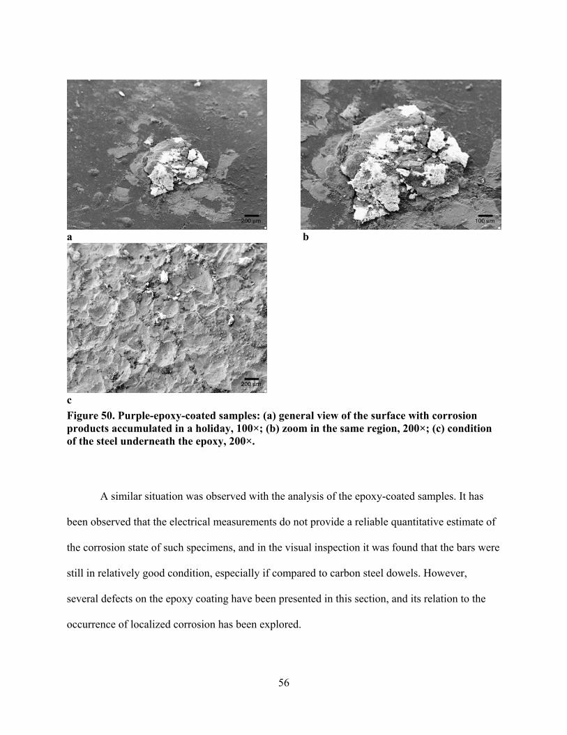
56
a b
c
Figure 50. Purple-epoxy-coated samples: (a) general view of the surface with corrosion products accumulated in a holiday, 100×; (b) zoom in the same region, 200×; (c) condition of the steel underneath the epoxy, 200×.
A similar situation was observed with the analysis of the epoxy-coated samples. It has
been observed that the electrical measurements do not provide a reliable quantitative estimate of
the corrosion state of such specimens, and in the visual inspection it was found that the bars were
still in relatively good condition, especially if compared to carbon steel dowels. However,
several defects on the epoxy coating have been presented in this section, and its relation to the
occurrence of localized corrosion has been explored.

57
3.3 Phase III Results
Six cores from the WSDOT slabs extracted and transported to California were also tested
in the Caltrans laboratory. Ten cores extracted from the corners of in-service pavements (two
from each of five locations in Washington State) were submitted to Construction Technology
Laboratories, Inc. for testing as well. The chloride contents of the concrete at different depths of
the cores were compared between the laboratory specimens and the field slabs to compare the
severity of the laboratory chloride environment to that of field slabs. This comparison helps to
place the results from the accelerated laboratory testing to long-term field conditions.
3.3.1 Extracted WSDOT Pavement Slabs
This section presents the results and discussion of half-cell potential tests, Linear
Polarization Resistance experiments, chloride analyses, and visual inspection performed on the
slabs from the WSDOT dowel bar retrofit project on Interstate 90.
3.3.1.1 Half-cell Potential and Linear Polarization Resistance
Figures 51 to 53 present the results of Linear Polarization Resistance tests done on the
extracted WSDOT slabs. In these plots, the current density (in µA/cm2) is plotted versus
potential (in mV), and the X-axis crosses the Y-axis at the half-cell potential value. The slope of
the curves (∆E/∆i) provides the value of the polarization resistance (Rp), with flatter slopes
indicating faster corrosion rate. The location of specimens A, B and C are illustrated in Figure
54.
Although the polarization resistance appears to be large when estimated by the Linear
Polarization Resistance method (which would lead to a small corrosion current density), it is
important to highlight that accelerated, localized corrosion may occur at defects and/or
underneath the epoxy coating. One has to keep in mind that this corrosion detection technique

58
y = 920.11x - 651.2R2 = 0.9728
-460
-450
-440
-430
-420
-410
-400
0.21 0.22 0.23 0.24 0.25 0.26 0.27
Current Density (µA/cm2)
Pote
ntia
l (m
V)
Figure 51. Linear Polarization Resistance, WSDOT slab, Specimen A.
y = 570.17x - 450.75R2 = 0.9818
-430
-420
-410
-400
-390
-380
-370
0.04 0.05 0.06 0.07 0.08 0.09 0.10 0.11 0.12 0.13
Current Density (µA/cm2)
Pote
ntia
l (m
V)
Figure 52. Linear Polarization Resistance, WSDOT slab, Specimen B.
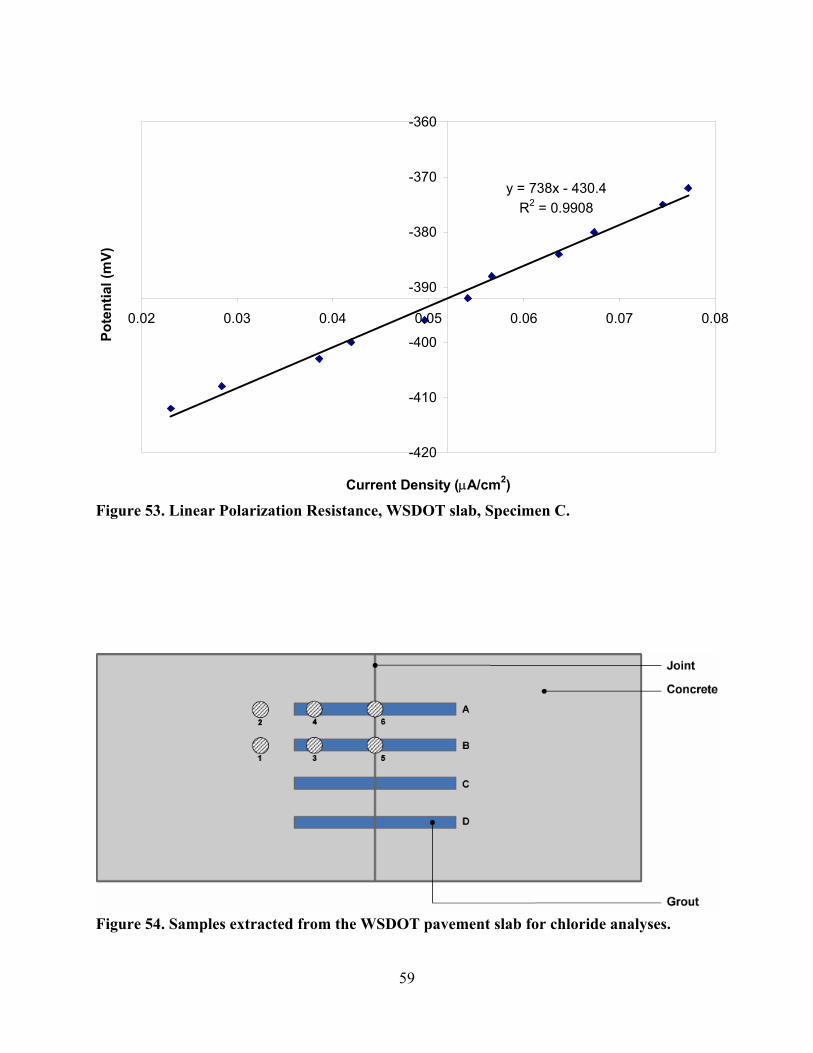
59
y = 738x - 430.4R2 = 0.9908
-420
-410
-400
-390
-380
-370
-360
0.02 0.03 0.04 0.05 0.06 0.07 0.08
Current Density (µA/cm2)
Pote
ntia
l (m
V)
Figure 53. Linear Polarization Resistance, WSDOT slab, Specimen C.
Figure 54. Samples extracted from the WSDOT pavement slab for chloride analyses.
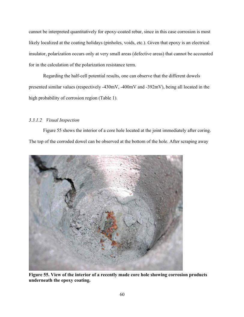
60
cannot be interpreted quantitatively for epoxy-coated rebar, since in this case corrosion is most
likely localized at the coating holidays (pinholes, voids, etc.). Given that epoxy is an electrical
insulator, polarization occurs only at very small areas (defective areas) that cannot be accounted
for in the calculation of the polarization resistance term.
Regarding the half-cell potential results, one can observe that the different dowels
presented similar values (respectively -430mV, -400mV and -392mV), being all located in the
high probability of corrosion region (Table 1).
3.3.1.2 Visual Inspection
Figure 55 shows the interior of a core hole located at the joint immediately after coring.
The top of the corroded dowel can be observed at the bottom of the hole. After scraping away
Figure 55. View of the interior of a recently made core hole showing corrosion products underneath the epoxy coating.

61
some of the loose epoxy coating, a considerable amount of corrosion product was found. The
core was removed using water for cooling the core bit, however, no time was permitted for
corrosion to occur because of the coring water.
The coring also revealed that one of the retrofit dowel bars was not centered over the
transverse joint, and only extended approximately 100 mm into the slab on one side of the joint.
It is certain that this misplacement of the dowel contributed to the low load transfer efficiency of
the joint. It is likely that the observed corrosion, and presence of the weak layer of corrosion
product between the concrete and the dowel also contributed to the loss of LTE.
3.4 Analysis of Chloride Contents
As mentioned in Section 2.6, several chloride analyses were performed on concrete cores
cut from: 1) extracted WSDOT pavement slabs, 2) near-joint corners of in-service slabs at five
different locations in Washington state, and 3) the laboratory beams from Phase II testing
exposed to 3.5% NaCl solution. Such chloride profiles are used to evaluate the concentration of
chlorides in the region surrounding the steel dowels, particularly in the vicinities of the open
joints, and to compare field and laboratory exposure conditions.
3.4.1 Chloride Analyses from WSDOT Slab Extracted from Interstate 90
As schematically represented in Figure 55, six samples were obtained from the extracted
WSDOT slabs from Interstate 90 for chloride analyses. Cores 1 and 2 were made through the
concrete only; cores 3 and 4 were cut through the retrofit grout and the end of the dowel, and
cores 5 and 6 were obtained at the joint through grout and the dowel. The samples were
submitted to the Caltrans chemistry laboratory for the analyses to be performed.

62
Core 4 (grout) could not be completely removed on the same day due to problems with
the coring machine, and was left out of the analyses. Results for Core 3 (Figure 58) showed that
the concentration of chlorides in this region was low, and attention was focused on the study of
chloride concentrations in the jointed region.
Figures 56 to 60 show the chloride profiles obtained for this pavement slab. The
pavement was built in 1964, and deicing salts were applied 120-150 days per year, with each icy
day typically having at least two applications. Details of location, salt usage and joint sealing
practices are presented in Table 9 (SR-90 MP 76.88, extracted slab).
The steel dowels are located approximately at 3 inches depth. It can be noticed that the
chloride concentration at this depth is around 1.0 lb./cu. yd., which is near the chloride threshold
for regular carbon steel found in the literature (7). Notice that sometimes a smaller concentration
may be verified at the top layer due to Cl- being “washed out” by surface water.
Figure 58 shows a profile of the chloride concentrations on the grout used for the dowel-
bar retrofit done in 1994. Even approximately 10-11 years after the project, one can observe that
the concentration of Cl- ions is considerably below the minimum value to initiate corrosion, even
for regular unprotected carbon steels. However, in Figures 59 and 60 it can be seen that the
chloride concentrations close to the joint are significantly higher, reaching values as high as
11.38 lb./cu. yd. along the profile and 8.43 lb./cu. yd. in a region close to the dowel (Figure 60).
The results presented in Figures 56-60 indicate that the chloride ions can more easily
penetrate the grout through the open joint. Thus, at the joint, easier access and accumulation of
chlorides results in higher localized concentrations close to the dowels. It is important to notice
that in this case the chloride ions do not infiltrate the concrete (or grout) from the top, but instead
they migrate through the open joint to the dowel.

63
0 2 4 6 8 10 12 14 16 18 20
0.16
0.31
0.47
0.63
0.79
0.94
1.10
1.26
1.42
1.57
1.73
1.89
2.05
2.20
2.36
2.76
Dep
th (i
n.)
[Cl-], lb./cu. yd.
Figure 56. Chloride profile of the slab concrete (Core #1).
0 2 4 6 8 10 12 14 16 18 20
0.160.310.470.630.790.941.101.261.421.571.731.892.052.202.362.522.682.95
Dep
th (i
n.)
[Cl-], lb./cu. yd.
Figure 57. Chloride profile of the slab concrete (Core #2).

64
0 2 4 6 8 10 12 14 16 18 20
0.16
0.31
0.47
0.63
0.79
0.94
1.10
1.26
1.42
1.57
1.73
1.89
2.05
2.20
2.76
Dep
th (i
n.)
[Cl-], lb./cu. yd.
Figure 58. Chloride profile of the grout used for dowel bar retrofit (Core #3).
0 2 4 6 8 10 12 14 16 18 20
0.16
0.31
0.47
0.63
0.79
0.94
1.10
1.26
1.42
1.57
1.73
2.76
Dep
th (i
n.)
[Cl-], lb./cu. yd.
Figure 59. Chloride profile of the grout around the pavement joint (Core #5).

65
0 2 4 6 8 10 12 14 16 18 20
0.16
0.31
0.47
0.63
0.79
0.94
1.10
1.26
1.42
1.57
1.73
1.89
2.05
2.20
2.76
Dep
th (i
n.)
[Cl-], lb./cu. yd.
Figure 60. Chloride profile of the grout around the pavement joint (Core #6).
3.4.2 Chloride Analyses of Cores from WSDOT Pavements in Various Locations
This section presents the results of the chloride analyses performed on cores extracted
from slab corners, next to the transverse joint of in-service slabs at five different locations in
Washington State. These cores were extracted by WSDOT and tested for chloride content by
CTL (Construction Technology Laboratories, Inc.) for comparison with the laboratory results.
Table 9 describes the locations from which cores were extracted, including years of construction
and salt usage and joint sealing practices. Figures 61-65 present the chloride concentration
profiles for the different locations described in Table 9. The error bars represent minimum and
maximum values obtained at each location.
It is interesting to notice that the concentration of 1.0 lb./cu. yd., regarded as the chloride
threshold for carbon steel, is exceeded in nearly all cases, except for the samples from Wapato

Table 9 Samples Extracted from In-service Pavements for Chloride Analyses (Information Provided by WSDOT) Route Number
Location (MP) Year Depth
(in) Salt Usage Joint Sealing
I-90 76.88 (extracted slab)
1964 9 Up until the early 1980’s, rock salt was used approximately 120-150 days per year at a typical rate of 180 pounds per mile using a 5:1 ratio (1 scoop of salt to 5 scoops of sand). Each day typically had at least two applications. Salting typically occurs from mid November to mid April. From the early 1980’s to 1997 or so, rust inhibitor type deicers/salts have been used. Since 1997 or so liquid magnesium chloride has been used at a typical rate of 35 gallons per mile with a range of 15 to 50. The average rate seems to be coming down with the use of better flow controls.
Sawed and sealed during initial construction with a rubberized joint sealer product called “Seal Target 164.” Joint sealed during 1994 DBR with rubberized joint sealant.
I-5 166.00 (Downtown Seattle)
1967 9 No data yet. Sawed and sealed during initial construction with a rubberized joint sealer product called “Seal Target 164.” No sealing since original construction.
I-90 91.324 (Elk Heights)
1967 9 See I-90 above. Same. Sawed and sealed during initial construction with a rubberized joint sealer product called “Seal Target 164.” Joint sealed during 1994 DBR with rubberized joint sealant with rubberized joint sealant.
I-90 61.304 (Price Creek)
1959 9 See I-90 above. Same. Sawed and sealed during initial construction with a rubberized joint sealer product called “Seal Target 164.” Joint sealed during 1997 DBR with rubberized joint sealant.
SR 82 10.617 (Military Road)
1971 9 Same as 1-90 above except that the use of rock salts was about 100 days per year. Most days had two applications. Rust inhibitor deicers/salts were used from the early 1980’s to 1997 or so. Since 1997 liquid magnesium chloride has been used at the typical rates reported above.
Sawed and sealed during initial construction with a rubberized joint sealer product called “Seal Target 164.” Joint sealed during 1997 DBR with rubberized joint sealant.
SR 82 43.524 (Wapato)
1981 9 Same as I-90 above, however the applications of rock salt were about 60-70 days per year until about 1985. Each day often had two applications. Rock salt was used at a 15:1 to a 20:1 blend. From 1985 to about 2000 rust inhibitor salts were used at the same rate. Since 2000, magnesium Chloride has been used.
Sawed and sealed during initial construction with a rubberized joint sealer product called “Seal Target 164.” No sealing since original construction.
66

67
0 - ¾"
¾" - 1½"
1½" - 2¼"
2¼" - 3"
3" - 3¾"
3¾" - 4½"
0 2 4 6 8 10 12 14 16 18 20D
epth
(in.
)[Cl-], lb./cu. yd.
Figure 61. Chloride profile for SR 5 MP 166.00 (downtown Seattle).
0 - ¾"
¾" - 1½"
1½" - 2¼"
2¼" - 3"
3" - 3¾"
3¾" - 4½"
0 2 4 6 8 10 12 14 16 18 20
Dep
th (i
n.)
[Cl-], lb./cu. yd.
Figure 62. Chloride profile for SR 90 MP 91.324 (Elk Heights).

68
0 - ¾"
¾" - 1½"
1½" - 2¼"
2¼" - 3"
3" - 3¾"
3¾" - 4½"
0 2 4 6 8 10 12 14 16 18 20D
epth
(in.
)[Cl-], lb./cu. yd.
Figure 63. Chloride profile for SR 90 MP 61.304 (Price Creek).
0 - ¾"
¾" - 1½"
1½" - 2¼"
2¼" - 3"
3" - 3¾"
3¾" - 4½"
0 2 4 6 8 10 12 14 16 18 20
Dep
th (i
n.)
[Cl-], lb./cu. yd.
Figure 64. Chloride profile for SR 82 MP 10.617 (Military Road).

69
0 - ¾"
¾" - 1½"
1½" - 2¼"
2¼" - 3"
3" - 3¾"
3¾" - 4½"
0 2 4 6 8 10 12 14 16 18 20D
epth
(in.
)[Cl-], lb./cu. yd.
Figure 65. Chloride profile for SR 82 MP 43.524 (Wapato).
(Figure 65), which is a more recently built pavement where deicing salts were applied only 60-
70 days/year at lower rates. Even so, at this location, [Cl-] reached 0.6-0.7 lb./cu. yd. On the
other hand, only the older pavement built in 1959 (Figure 63), which was exposed to two daily
applications of deicing salts for 120-150 days/year, reached a concentration that was high enough
to overcome the chloride threshold of 7.7 lb./cu. yd. found in the references for the
microcomposite steel (7-9).
3.4.3 Chloride Analyses from Laboratory Samples
As described in Section 2.6, cylindrical cores were extracted from the laboratory concrete
beams at the central, jointed region. The laboratory specimens were subjected to wet-and-dry
cycles with a 3.5% NaCl solution, which is typically used to simulate seawater, over an 18-

70
month period. The extracted samples were shipped to the Caltrans chemistry laboratory where
the [Cl-] analyses were performed. Figures 66-71 present the results from these analyses.
In general, it can be seen that the chloride concentrations are much more constant along
the depth profile, as compared to situations in which the chloride has to diffuse through the
concrete (e.g., Figures 57 and 58) or migrate through a narrow joint (e.g., Figures 60 and 63).
This is due to the fact that in the laboratory specimens, a large (approximately 6 × 50mm) open
joint was cast above the dowels.
In addition, it was verified that the use of a 3.5% NaCl solution may lead to high chloride
concentrations, as compared to the results obtained in the field specimens, greatly accelerating
the corrosion process. As a result of this aggressive environment, corrosion could be observed in
nearly all samples after only 18 months of exposure, except for the stainless clad and stainless
0 4 8 12 16 20 24 28 32 36 40
0.16
0.31
0.47
0.63
0.79
0.94
1.10
1.26
1.42
1.57
1.73
1.89
2.05
2.20
2.36
Dep
th (i
n.)
[Cl-], lb./cu. yd.
Figure 66. Chloride profile on the concrete of a carbon steel specimen.

71
0 4 8 12 16 20 24 28 32 36 40
0.160.310.470.630.790.941.101.261.421.571.731.892.052.202.362.522.682.83
Dep
th (i
n.)
[Cl-], lb./cu. yd.
Figure 67. Chloride profile on the concrete of a stainless clad specimen.
0 4 8 12 16 20 24 28 32 36 40
0.16
0.31
0.47
0.63
0.79
0.94
1.10
1.26
1.42
1.57
1.73
1.89
2.05
2.20
Dep
th (i
n.)
[Cl-], lb./cu yd.
Figure 68. Chloride profile on the concrete of a stainless hollow specimen.

72
0 4 8 12 16 20 24 28 32 36 40
0.16
0.31
0.47
0.63
0.79
0.94
1.10
1.26
1.42
1.57
1.73
1.89
2.05
Dep
th (i
n.)
[Cl-], lb./cu yd.
Figure 69. Chloride profile on the concrete of a flexible (green) epoxy-coated specimen.
0 4 8 12 16 20 24 28 32 36 40
0.16
0.31
0.47
0.63
0.79
0.94
1.10
1.26
1.42
1.57
1.73
1.89
2.05
2.20
2.36
2.52
Dep
th (i
n.)
[Cl-], lb./cu. yd.
Figure 70. Chloride profile on the concrete of a non-flexible (purple) epoxy-coated specimen.
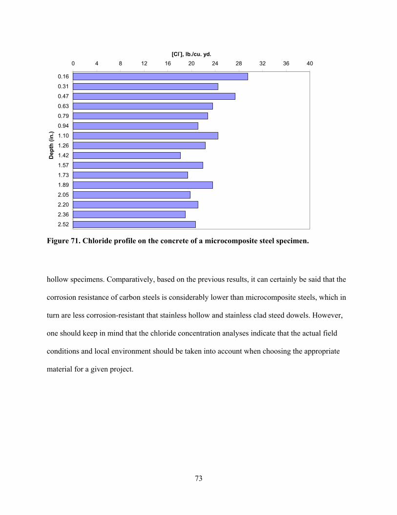
73
0 4 8 12 16 20 24 28 32 36 40
0.16
0.31
0.47
0.63
0.79
0.94
1.10
1.26
1.42
1.57
1.73
1.89
2.05
2.20
2.36
2.52
Dep
th (i
n.)
[Cl-], lb./cu. yd.
Figure 71. Chloride profile on the concrete of a microcomposite steel specimen.
hollow specimens. Comparatively, based on the previous results, it can certainly be said that the
corrosion resistance of carbon steels is considerably lower than microcomposite steels, which in
turn are less corrosion-resistant that stainless hollow and stainless clad steed dowels. However,
one should keep in mind that the chloride concentration analyses indicate that the actual field
conditions and local environment should be taken into account when choosing the appropriate
material for a given project.

74

75
4.0 CONCLUSIONS AND RECOMMENDATIONS
This study investigated the corrosion performance of several types of steel dowels cast in
concrete beams through the use of accelerated laboratory tests. The accelerated testing consisted
of ponding water with a chloride solution on the top of the beams and including a “joint” in each
beam that provided direct access to a short segment of the dowels. No force loading was applied
to the beams. Results are presented from the tests.
Conclusions are based on the results of half-cell potential tests, Linear Polarization
Resistance curves, visual inspections, and microscopic investigations by Scanning Electron
Microscope (SEM), all of which are presented in this report.
4.1 Phase I Testing Conclusions
The following conclusions are from the Phase I testing consisting of placement of four
types of dowels (carbon steel, epoxy-coated steel, stainless steel hollow, and stainless steel clad)
cast in concrete beams with joints in different corrosive environments, and evaluation using half-
cell potential tests for corrosion initiation and visual inspection at the completion of testing.
1. Carbon steel dowels present the shortest corrosion initiation period—when chlorides
have direct access to the bar through the joint, the initiation stage can be disregarded
and the corrosion propagation phase begins immediately. Epoxy-coated dowels
increased the initiation period considerably, while the stainless hollow and stainless
clad dowels provided the highest resistance to the onset of corrosion.
2. From the visual inspections after 6 months of cyclic ponding, it was observed that the
carbon steel dowels present uniform corrosion along the bar, while epoxy-coated
dowels had localized corrosion at defects mostly at the ends of the bars where the
76
coating is most vulnerable to damage. No visible corrosion was found on either the
stainless steel hollow bars or stainless clad bars.
4.2 Phase II Testing Conclusions
The following conclusions are based on the Phase II laboratory testing in which seven
types of dowels (carbon steel, microcomposite steel, stainless steel hollow, stainless steel clad,
carbon steel coated with flexible epoxy (green colored), and carbon steel coated with non-
flexible epoxies (purple and gray colored)) were cast in concrete beams with joints in different
corrosive environments. These specimens were evaluated for corrosion resistance using half-cell
potential tests, Linear Polarization Resistance curves, visual inspections, chloride analyses, and
microscopic investigations.
1. In coated specimens, such as the epoxy-coated specimens included in this study,
corrosion is not uniform, but is instead concentrated at localized defective areas (such
as pinholes, voids, etc.). Given that epoxy is an electrical insulator, polarization
happens only at very small areas (defective areas) that cannot be accounted for in the
calculation of the polarization resistance term. Therefore, the epoxy-coated dowels
cannot be quantitatively evaluated with the other dowels and must be evaluated
qualitatively.
2. The carbon steel dowels exhibited the lowest values of polarization resistance (Rp)
and therefore have the smallest resistance to charge transfer across the interface, and
are therefore expected to have the fastest rate of corrosion propagation
3. Microcomposite steel dowels exhibited polarization resistance (Rp) approximately 35
times greater than carbon steel dowels, while stainless clad and stainless hollow bars
had about 73 times greater polarization resistance. Notice that Rp is inversely

77
proportional to the corrosion current density, and thus to the corrosion rate (see
Equations A1 and A2 in Appendix A). This indicates that the microcomposite steel
dowels exhibit much greater resistance to corrosion propagation than carbon steel
dowels, but not as much as the stainless clad and hollow bars.
4. Based on corrosion current density results, it was verified that the carbon steel dowels
exhibited very rapid corrosion, while microcomposite steel exhibited a moderate level
and stainless steel clad and stainless steel hollow proceeded at a low corrosion rate.
5. Visual inspections of the corroded dowels revealed heavy and mostly uniform
corrosion along the carbon steel dowels, light corrosion in the microcomposite steel
dowels, and no visible corrosion in the stainless steel clad and stainless steel hollow
bars. For the epoxy-coated dowels, the visual inspections generally revealed that
visible corrosion was not widespread, but did occur at a few localized defective areas,
generally at holidays and at the edges of the bar ends. No significant difference was
observed on the performance of non-flexible and flexible epoxy-coated dowels.
6. In general, the microscopic investigation by SEM matches well the results anticipated
by the electrical measurements and visual inspections. However, the analysis has
focused mostly on the corroded areas of each sample, and revealed corroded areas
that were not visible to the naked eye.
7. Statistical analyses of the results show that, in all cases, the type of steel dowel have a
statistically significant effect on the quantitative parameters studied (i.e., half-cell
potential, polarization resistance, and corrosion current density).

78
4.3 Conclusions from Phase III Testing
The following conclusions are drawn from the Phase III evaluation of the WSDOT dowel
bar retrofit slabs extracted from the 40-year old field section.
1. In the extracted slabs from which cores were taken at the joints, a considerable
amount of corrosion product was verified by means of visual inspection. The
corrosion occurred underneath the epoxy coating on the central region of the dowel
beneath the joint. The corrosion is likely to have contributed to the loss of load
transfer efficiency of the joint because of the low strength corrosion products at the
interface between the concrete and the dowel. Lack of centering of one dowel over
the transverse joint is also likely to have contributed to the low LTE.
2. Half-cell potential and Linear Polarization Resistance results match the visual
observations, indicating the presence of active corrosion.
4.4 Conclusions from Chloride Analysis
The following conclusions are made regarding the relationship among the concentrations
of chlorides in the laboratory samples, extracted WSDOT field slabs, and cores extracted from
slabs in various locations in Washington State:
1. Chloride concentrations close to the pavement joints are significantly higher than in
other regions of the pavement. At the joint, easier access and accumulation of
chlorides leads to higher, localized concentrations.
2. When a joint is present, the chloride ions do not reach the dowel through the concrete
(or grout) from the top, rather, they migrate through the open joint to the dowel.
3. In the field experiments, it was verified that the chloride threshold for carbon steel
was exceeded in five out of six projects.
79
4. In the laboratory samples, with open joints located above the dowels, the chloride
concentrations are more constant along the depth profile, as compared to field
conditions in which the chloride have to diffuse through the concrete or migrate
through a narrower joint.
5. The use of a 3.5% NaCl solution for laboratory experiments may lead to considerably
high chloride concentrations, as compared to the results obtained in the field
specimens, greatly accelerating the corrosion process. As a result of this aggressive
environment, corrosion could be observed in nearly all samples in only 18 months of
exposure.
6. Laboratory results can be used to comparatively evaluate the corrosion resistance of
different materials when exposed to the same aggressive environment. However, the
chloride concentration analyses indicate that the actual field conditions and local
environment should be taken into account when choosing the appropriate material for
a given project.
4.5 Recommendations
The following recommendations are based on the conclusions presented above.
1. The presence of corrosion at the ends and along the length of a dowel from ponding
water on cast in concrete dowels indicates that chlorides can pass all the way to the
dowel ends from the joint along the horizontal interface between the dowel and the
concrete, or through the concrete. For this reason it is recommended that uncoated
carbon steel dowels not be used.
2. Epoxy dowels present some risk of corrosion, primarily localized at holidays and the
ends. Based on this finding, it is recommend that

80
1. Quality control checks to control holidays should be implemented.
2. Bar ends should be coated with epoxy, and care must be taken with epoxy-coated
dowels during shipping, storage, and installation. Corrosion will be exacerbated if
the bar ends are not coated (observed on various Caltrans construction sites) or if
the coated ends are damaged during storage, transport and installation.
3. It is recommended that the use of stainless steel clad, hollow stainless steel, or
microcomposite steel dowels be considered for locations with high risk of high
chloride exposure (such as on mountain passes and marine environments), where
exposure to corrosive water is anticipated. The selection of a specific corrosion
resistant dowel should be based on further field investigations and cost differences.
4. It is recommended that a field study be performed at several mountain pass locations
to measure the chloride content of snow melt after sand/salt application for
comparison with the chloride content of the solution used in the laboratory testing in
Phases I and II. The results of this study should be used to further refine the risk
assessment in these critical locations.

81
5.0 REFERENCES
1. Harvey, J. T., A. Ali, D. Hung, J. Uhlmeyer, L Popescu, D. Bush, K Grote, J. Lea, C. Scheffy. Construction and Test Results from Dowel Bar Retrofit HVS Test Sections 553FD, 554FD and 555FD: US 101, Ukiah, Mendocino County. Draft report prepared for the California Department of Transportation. Pavement Research Center, Institute of Transportation Studies, University of California. February 2003.
2. Bentur, A., S. Diamond, N.S. Berke. Steel Corrosion in Concrete. E&FN Spon, 1997.
3. Mehta, P.K. and P.J.M. Monteiro. Concrete: Structure, Properties and Materials. 2nd Edition, McGraw Hill, 1993.
4. Davids, W.G., Z.M. Wang, G. Turkiyyah, J. Mahoney, and D. Bush. “3D Finite Element Analysis of Jointed Plain Concrete Pavement with EverFE2.2.” Transportation Research Record 1853, TRB, National Research Council, Washington, D.C., 2003, pp 92-99.
5. Mack, J.W. “Dowel Retrofit Restores Pavement Load Transfer.” American Concrete Paving Association. Available online at http://www.pavement.com/PavTech/Tech/Dwnlds/DwnldPubs.html
6. Tuutti, K. Corrosion of Steel in Concrete. Stockholm (in Swedish). Cement and Concrete Research Institute, 1982.
7. Trejo, D.; Radhakrishna, P. Evaluation of the Critical Chloride Threshold for Different Steel Reinforcement Types. TEES/MMFX Final Report. Texas Engineering Experiment Station, Texas A&M University, March 2005.
8. Trejo, D.; Radhakrishna, P. “Accelerated Chloride Threshold Testing: Part I – ASTM A 615 and A 706 Reinforcement.” ACI Materials Journal, 100 (6). 2003. pp.519-527.
9. Trejo, D.; Radhakrishna, P. “Accelerated Chloride Threshold Testing: Part I – Corrosion Resistant Reinforcement.” ACI Materials Journal, 101 (1). 2004. pp.57-64.
10. Trejo, D. Microstructural Design and Electrochemical Evaluation of Dual-phase Ferritic Martensitic Steel for Concrete Reinforcement. Ph.D. Dissertation, University of California, Berkeley, California, 1997.
11. Trejo, D.; P.J.M. Monteiro, B.C. Gerwick, and G. Thomas. “Microstructural Design of Concrete Reinforcing Bars for Improved Corrosion Performance.” ACI Materials Journal, 97 (1). 2000. pp.78-83.
12. Carino, N.J. “Nondestructive Techniques to Investigate Corrosion Status in Concrete Structures.” Journal of Performance of Constructed Facilities, 13 (3). 1999. pp.96-106.
13. Broomfield, J.P. Corrosion of Steel in Concrete: Understanding, Investigation and Repair. E&FN Spon, 1997.

82
14. Vesilind, P.A. Introduction to Environmental Engineering. PWS Publishing Company, Boston, 468 pages, 1996.
15. Lee, S-K, and P.D. Kraus. Long-Term Performance of Epoxy-Coated Reinforcing Steel in Heavy Salt-Contaminated Concrete. FHWA Publication No. FHWA-HRT-04-090.
16. Pavement Systems Limited LLC. Climatic Database for Integrated Model (CDIM). Software, version 1.0. Prepared for California Department of Transportation under contract to University of California Partnered Pavement Research Center. Bethesda, MD. April, 2004.

A-1
APPENDIX A: DETECTION TECHNIQUES
Half-cell Potential
The standard test method for half-cell potential measurements is described in ASTM C
876 (1997). The test apparatus (illustrated in A1) consists of an external electrode (half cell)1,
connecting wires, and a high impedance voltmeter (impedance >10MΩ). The high impedance
voltmeter is used so that there is a very little current through the circuit.
The half-cell potential measurement has been widely used in the field, due to its
simplicity and general agreement that this technique does indicate the existence of active
corrosion along the steel reinforcement in concrete.
Note that one terminal of the voltmeter must be connected to the reinforcement, that is,
physical access to the reinforcement must be provided, so it is usual practice to break away the
concrete cover to enable the electrical contact to be made.
When active corrosion is present, current flows through the concrete between the anodic
and cathodic sites due to the migration of ions, and this current is accompanied by an electrical
potential field surrounding the corroding bar. Also, once the metal used for the half-cell electrode
(silver, mercury, or copper) has a more positive standard potential than iron, the external
electrode will be the cathode in the circuit (Figure A1).
1 The most commonly used electrodes are: silver/ silver chloride (Ag/AgCl), mercury/mercury oxide (Hg/HgO) and copper/copper sulfate (Cu/CuSO4). In laboratory, it is more usual to measure potentials with a calomel electrode (mercury/mercury chloride).

A-2
Figure A1. Apparatus for half-cell potential measurement, described in ASTM C 876.
So, if the bar is corroding, the excess electrons in the bar will tend to flow from the bar
(anode) to the half-cell (cathode). Because of the way the terminals of the voltmeter are
connected, the voltmeter indicates a negative voltage. A more negative voltage reading is
interpreted to mean that the embedded bar has more excess electrons and, therefore, there is a
higher likelihood that the bar is corroding. The half-cell potential measurements are indicative of
the probability of corrosion activity of the reinforcing steel located beneath the half-cell. (12, 13)
The appendix of ASTM C 876 provides guidelines on interpreting results obtained
through half-cell potential measurements. There are two basic techniques to evaluate the results:
the numerical technique, in which the value of the potential is used as an indicator of the

A-3
likelihood of corrosion activity (see Table A1); and the potential difference technique, in which
the areas of active corrosion are identified on the basis of the potential gradients, constructed
based on an equipotential contour plot.
Table A1 Relationship between Half-cell Potential and Corrosion of Steel Embedded in Concrete (ASTM C 876)
Half-cell potential (mV) * Interpretation > -200 Low probability (10%) of corrosion -200 to -350 Corrosion activity (uncertain) < -350 High probability (90%) of corrosion) *Measurements made with a copper/ copper sulfate electrode. According to Carino, it is generally accepted that the potential difference technique is
more reliable for identifying regions of active corrosion than is the use of numerical limits.(12)
Thus, the half-cell potential method provides an indication of the likelihood of corrosion activity
at the time of the measurement. However, it does not give any information on the rate of
corrosion of the reinforcement.
Linear Polarization Resistance (LPR)
Several methods have been investigated for measuring the in-situ corrosion rate of steel
embedded in concrete. Among these methods, Linear Polarization Resistance (LPR) appears to
be gaining most acceptance.(12)
LPR is a well-established method for determining corrosion rate by using electrolytic test
cells (ASTM G 59). The technique involves measuring the change in the open-circuit potential of
the electrolytic cell when an external current is applied to the cell. For a small perturbation about
the open-circuit potential, there is a linear relationship between the change in applied current per
unit area of electrode (∆i) and the change in the measured voltage (∆E). The ratio ∆E/∆i is called
the polarization resistance (Rp). The corrosion rate, expressed as the corrosion current density, is
inversely related to the polarization resistance (ASTM G 59), as showed in Equation A1.

A-4
P
corr RBi = (A1)
In this equation, icorr is the corrosion current density (in A/cm2), B is a constant (in V) and
Rp is the polarization resistance (in Ω/cm2). The constant B is a characteristic of the polarization
curves, and a value of 26mV is commonly used for steel that is actively corroding in concrete.
The basic apparatus utilized is shown in Figure A2a.
One electrode is a reference half-cell, and the reinforcement is a second electrode called
the working electrode. The third electrode is referred to as the counter electrode, and it supplies
the polarization current to the bar. Supplementary instrumentation measures the voltages and
currents during different stages of the test.
A major concern with this method is the uncertainty regarding the area of the steel bar
that is affected by the current from the counter electrode. Usually it is assumed that the current
flows in straight lines perpendicular to the bar and the counter electrode, and the affected bar
area is taken as the bar circumference multiplied by the length of the bar below the counter
electrode. In the laboratory experiments performed as part of this study, the counter electrode
(CE) was placed above the joint, and therefore this concern is not justified. In this case, virtually
a b Figure A2. Three-electrode Linear Polarization Resistance method. (a) Measurement of the open-circuit potential (half-cell potential); (b) Current applied to the counter electrode to produce a small change in voltage ∆E.(12)

A-5
all the current will flow through the NaCl solution present in the open joint, which represents a
very low-resistivity path as compared to concrete.
Some guidelines have been developed to establish a relationship between corrosion
current density and corrosion speed, as can be seen in Table A2.(13)
Table A2 Relationship between Corrosion Current Density and Corrosion Speed Corrosion current density (µA/cm2) * Corrosion speed < 0.1 Negligible 0.1 – 0.5 Low 0.5 – 1.0 Moderate > 1.0 High *Measurements made with a guard electrode device.
Using Faraday’s law, the corrosion current density (Equation A1) can be converted to metal loss.
Faraday’s law can be expressed as
Fz
tiMm.
..= (A2)
In this equation, m is the mass of steel consumed, i is the current (in amperes), t is the
time (in seconds), F is Faraday’s constant (96500A), z is the ionic charge (equal to 2 for Fe
Fe+2 + 2e-), and M is the atomic weight of the metal (equal to 56g for Fe). This gives a
conversion of 1µA.cm2 = 11.6µm = 1.16*10-2 mm of steel section loss per year. It is important to
note that this calculation assumes that corrosion is occurring uniformly on the bar, which is the
typical condition when the corrosion is induced by a carbonation front. However, chloride-
induced corrosion is associated with small, concentrated areas of corrosion. It has been reported
that the depth of local pitting may be four to eight times the average depth of corrosion (12).
A-6
Physical Inspection
In addition to the electrochemical techniques, physical techniques have also found wide
application for detecting corrosion in reinforced concrete. Physical methods such as visual
inspection and others (e.g., stress wave techniques, magnetic methods, radar) can be used to
detect deterioration of concrete or reinforcement loss by corrosion. Most of these techniques
have been translated from concrete technology, where they were originally used for concrete
inspection of concrete degradation. Thus, most aim to detect corrosion from the identification of
damage to concrete, and other tests are usually needed to confirm the source and cause of the
deterioration (13). In the present study, the concrete samples were broken apart and direct visual
inspection was made on the corroded dowels.

B-1
APPENDIX B: LINEAR POLARIZATION RESULTS OF INDIVIDUAL SPECIMENS
Linear Polarization ResistanceCarbon Steel - 1
y = 1.5443x - 615.68R2 = 0.9822
-632
-622
-612
-602
-592
-582
-572
-10 -5 0 5 10 15 20 25
Current Density (µA/cm2)
Pote
ntia
l (m
V)
Linear Polarization ResistanceCarbon Steel - 2
y = 6.0665x - 643.73R2 = 0.9955
-670
-660
-650
-640
-630
-620
-610
-4.0 -3.0 -2.0 -1.0 0.0 1.0 2.0 3.0 4.0
Current Density (µA/cm2)
Pote
ntia
l (m
V)

B-2
Linear Polarization ResistanceCarbon Steel - 3
y = 2.5682x - 699.5R2 = 0.9894
-720
-710
-700
-690
-680
-670
-10 -5 0 5 10
Current Density (µA/cm2)
Pote
ntia
l (m
V)
Linear Polarization Resistance
Carbon Steel - 4
y = 5.4108x - 631.33R2 = 0.984
-660
-650
-640
-630
-620
-610
-600
-5 -4 -3 -2 -1 0 1 2 3 4 5
Current Density (µA/cm2)
Pote
ntia
l (m
V)

B-3
Linear PolarizationMicrocomposite - 1
y = 23.495x - 572.9R2 = 0.9559
-600
-590
-580
-570
-560
-550
-540
-1.0 -0.8 -0.6 -0.4 -0.2 0.0 0.2 0.4 0.6 0.8 1.0
Current density (µA/cm2)
Po
ten
tial
(m
V)
Linear PolarizationMicrocomposite - 2
y = 23.146x - 567.8R2 = 0.9611
-600
-590
-580
-570
-560
-550
-540
-1.4 -1.2 -1.0 -0.8 -0.6 -0.4 -0.2 0.0 0.2 0.4 0.6 0.8
Current density (µA/cm2)
Po
ten
tial
(m
V)
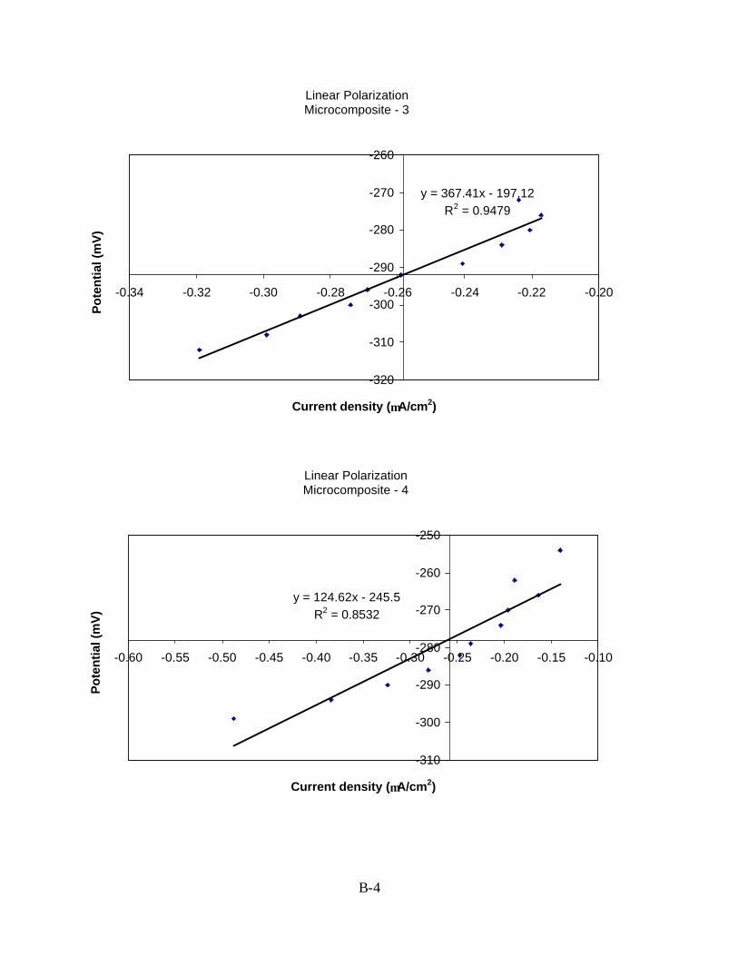
B-4
Linear PolarizationMicrocomposite - 3
y = 367.41x - 197.12R2 = 0.9479
-320
-310
-300
-290
-280
-270
-260
-0.34 -0.32 -0.30 -0.28 -0.26 -0.24 -0.22 -0.20
Current density (µA/cm2)
Po
ten
tial
(m
V)
Linear PolarizationMicrocomposite - 4
y = 124.62x - 245.5R2 = 0.8532
-310
-300
-290
-280
-270
-260
-250
-0.60 -0.55 -0.50 -0.45 -0.40 -0.35 -0.30 -0.25 -0.20 -0.15 -0.10
Current density (µA/cm2)
Po
ten
tial
(m
V)
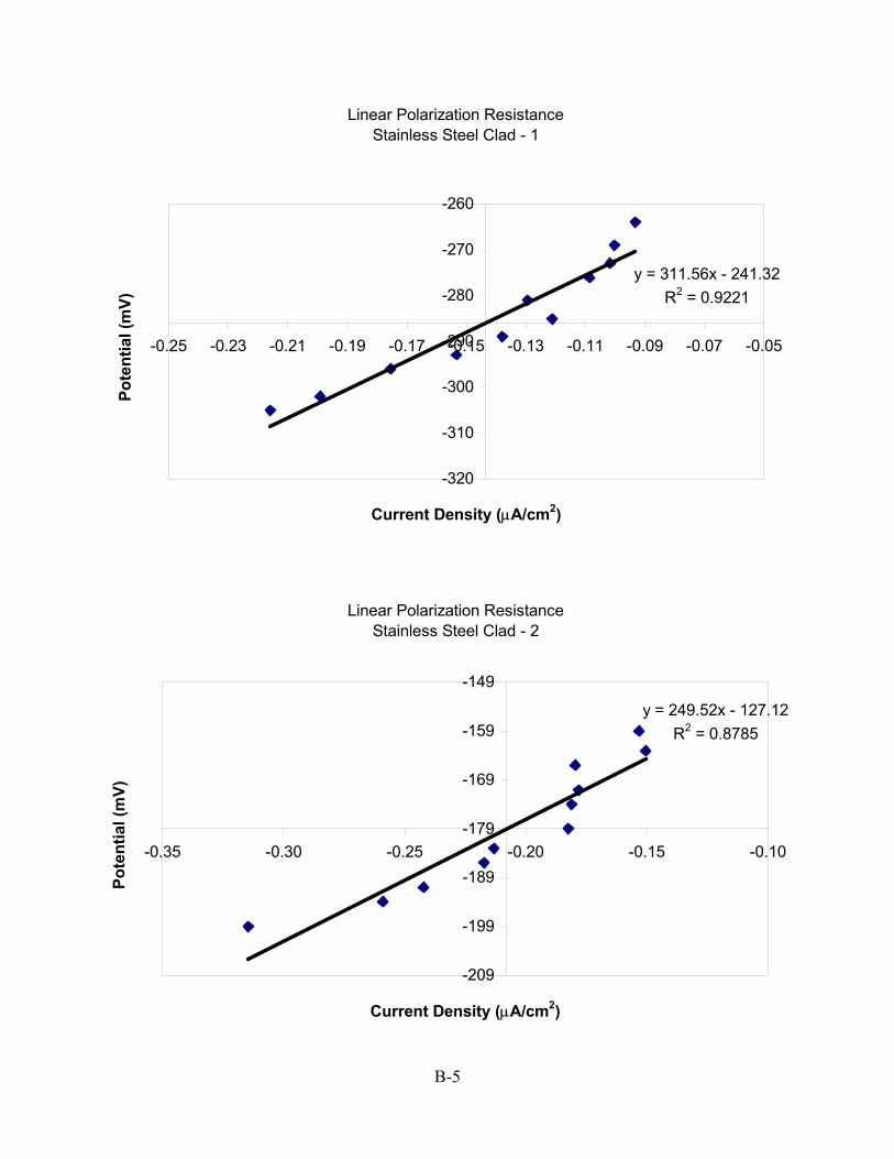
B-5
Linear Polarization ResistanceStainless Steel Clad - 1
y = 311.56x - 241.32R2 = 0.9221
-320
-310
-300
-290
-280
-270
-260
-0.25 -0.23 -0.21 -0.19 -0.17 -0.15 -0.13 -0.11 -0.09 -0.07 -0.05
Current Density (µA/cm2)
Pote
ntia
l (m
V)
Linear Polarization ResistanceStainless Steel Clad - 2
y = 249.52x - 127.12R2 = 0.8785
-209
-199
-189
-179
-169
-159
-149
-0.35 -0.30 -0.25 -0.20 -0.15 -0.10
Current Density (µA/cm2)
Pote
ntia
l (m
V)

B-6
Linear Polarization ResistanceStainless Steel Clad - 3
y = 361.13x - 141.12R2 = 0.9016
-250
-240
-230
-220
-210
-200
-190
-0.28 -0.26 -0.24 -0.22 -0.20 -0.18 -0.16
Current Density (µA/cm2)
Pote
ntia
l (m
V)
Linear Polarization ResistanceStainless Steel Clad - 4
y = 216.53x - 299.52R2 = 0.9075
-380
-370
-360
-350
-340
-330
-320
-0.35 -0.30 -0.25 -0.20 -0.15 -0.10
Current Density (µA/cm2)
Pote
ntia
l (m
V)
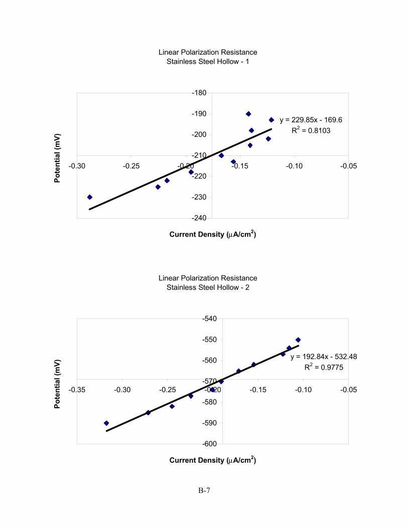
B-7
Linear Polarization ResistanceStainless Steel Hollow - 1
y = 229.85x - 169.6R2 = 0.8103
-240
-230
-220
-210
-200
-190
-180
-0.30 -0.25 -0.20 -0.15 -0.10 -0.05
Current Density (µA/cm2)
Pote
ntia
l (m
V)
Linear Polarization ResistanceStainless Steel Hollow - 2
y = 192.84x - 532.48R2 = 0.9775
-600
-590
-580
-570
-560
-550
-540
-0.35 -0.30 -0.25 -0.20 -0.15 -0.10 -0.05
Current Density (µA/cm2)
Pote
ntia
l (m
V)
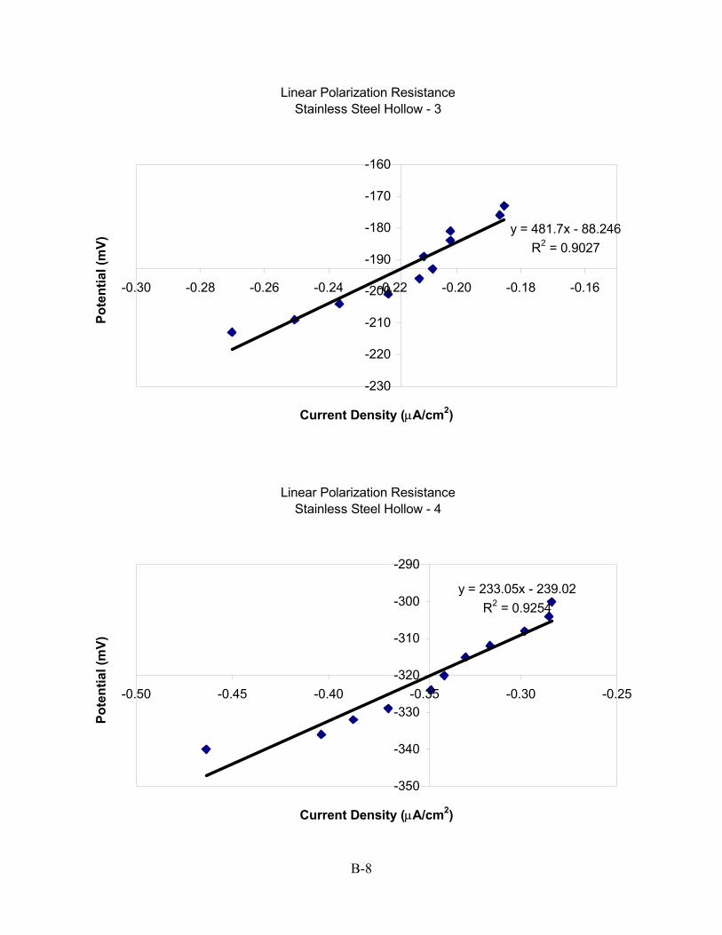
B-8
Linear Polarization ResistanceStainless Steel Hollow - 3
y = 481.7x - 88.246R2 = 0.9027
-230
-220
-210
-200
-190
-180
-170
-160
-0.30 -0.28 -0.26 -0.24 -0.22 -0.20 -0.18 -0.16
Current Density (µA/cm2)
Pote
ntia
l (m
V)
Linear Polarization ResistanceStainless Steel Hollow - 4
y = 233.05x - 239.02R2 = 0.9254
-350
-340
-330
-320
-310
-300
-290
-0.50 -0.45 -0.40 -0.35 -0.30 -0.25
Current Density (µA/cm2)
Pote
ntia
l (m
V)

B-9
Linear Polarization ResistancePurple Epoxy (Non-flexible) - 1
y = 72.432x - 463.42R2 = 0.986
-510
-500
-490
-480
-470
-460
-450
-0.50 -0.40 -0.30 -0.20 -0.10 0.00 0.10
Current Density (µA/cm2)
Pote
ntia
l (m
V)
Linear Polarization ResistancePurple Epoxy (Non-flexible) - 2
y = 992.03x - 358.25R2 = 0.8704
-610
-600
-590
-580
-570
-560
-0.25 -0.24 -0.23 -0.22 -0.21 -0.20
Current Density (µA/cm2)
Pote
ntia
l (m
V)

B-10
Linear Polarization ResistancePurple Epoxy (Non-flexible) - 3
y = 626.38x - 334.1R2 = 0.1037
-490
-480
-470
-460
-450
-440
-0.23 -0.22 -0.21 -0.20 -0.19
Current Density (µA/cm2)
Pote
ntia
l (m
V)
Linear Polarization ResistancePurple Epoxy (Non-flexible) - 4
y = 34.664x - 802.39R2 = 0.999
-840
-830
-820
-810
-800
-790
-780
-1.00 -0.80 -0.60 -0.40 -0.20 0.00 0.20 0.40
Current Density (µA/cm2)
Pote
ntia
l (m
V)
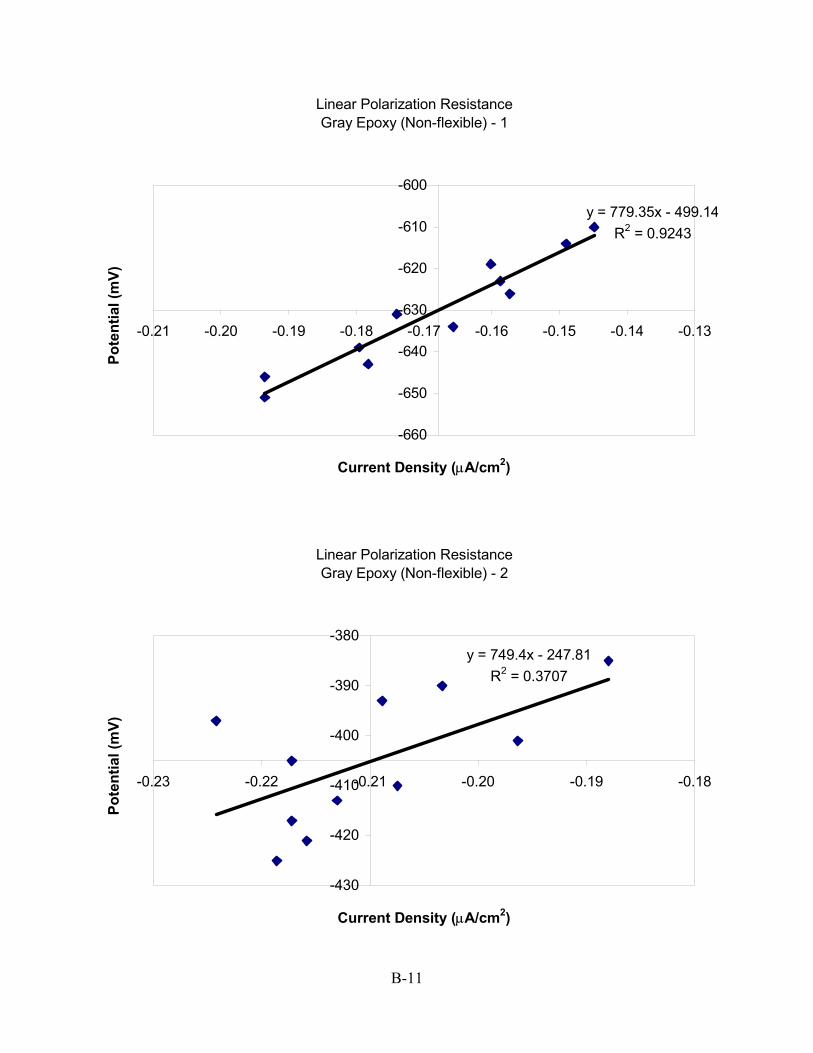
B-11
Linear Polarization ResistanceGray Epoxy (Non-flexible) - 1
y = 779.35x - 499.14R2 = 0.9243
-660
-650
-640
-630
-620
-610
-600
-0.21 -0.20 -0.19 -0.18 -0.17 -0.16 -0.15 -0.14 -0.13
Current Density (µA/cm2)
Pote
ntia
l (m
V)
Linear Polarization ResistanceGray Epoxy (Non-flexible) - 2
y = 749.4x - 247.81R2 = 0.3707
-430
-420
-410
-400
-390
-380
-0.23 -0.22 -0.21 -0.20 -0.19 -0.18
Current Density (µA/cm2)
Pote
ntia
l (m
V)

B-12
Linear Polarization ResistanceGray Epoxy (Non-flexible) - 3
y = 107.24x - 627.02R2 = 0.9733
-680
-670
-660
-650
-640
-630
-620
-0.50 -0.40 -0.30 -0.20 -0.10 0.00
Current Density (µA/cm2)
Pote
ntia
l (m
V)
Linear Polarization ResistanceGray Epoxy (Non-flexible) - 4
y = 331.55x - 527.91R2 = 0.0269
-620
-610
-600
-590
-580
-570
-0.23 -0.23 -0.22 -0.22 -0.21 -0.21 -0.20
Current Density (µA/cm2)
Pote
ntia
l (m
V)

B-13
Linear Polarization ResistanceGreen Epoxy (Flexible) - 1
y = 66.339x - 409.14R2 = 0.001
-460
-450
-440
-430
-420
-410
-400
-390
-380
-0.18 -0.17 -0.16 -0.15 -0.14
Current Density (µA/cm2)
Pote
ntia
l (m
V)
Linear Polarization ResistanceGreen Epoxy (Flexible) - 2
y = 120.62x - 735.68R2 = 0.9496
-790
-780
-770
-760
-750
-740
-730
-0.45 -0.40 -0.35 -0.30 -0.25 -0.20 -0.15 -0.10 -0.05 0.00
Current Density (µA/cm2)
Pote
ntia
l (m
V)

B-14
Linear Polarization ResistanceGreen Epoxy (Flexible) - 3
y = 669.91x - 411.68R2 = 0.3206
-590
-580
-570
-560
-550
-540
-530
-0.25 -0.25 -0.24 -0.24 -0.23 -0.23 -0.22 -0.22 -0.21 -0.21
Current Density (µA/cm2)
Pote
ntia
l (m
V)
Linear Polarization ResistanceGreen Epoxy (Flexible) - 4
y = 1106.5x - 389.5R2 = 0.9053
-670
-660
-650
-640
-630
-620
-0.25 -0.25 -0.24 -0.24 -0.23 -0.23 -0.22 -0.22 -0.21
Current Density (µA/cm2)
Pote
ntia
l (m
V)

C-1
APPENDIX C: CONCRETE MIX PROPORTIONS
Phase I Mix Proportions
Material Content (kg/m3)
Content (lb./cu. yd.)
Unit Proportions
Cement 399 672 1.00 Fine Aggregate 734 1237 1.84
Coarse Aggregate Total
Aggregate 1100 1834 1855 3092 2.76 4.60
Water 167 282 0.42 Phase II Mix Proportions
Material Content (kg/m3)
Content (lb./cu. yd.)
Unit Proportions
Cement 313 527 1.00 Fine Aggregate 939 1582 3.00
Coarse Aggregate Total
Aggregate 1017 1956 1714 3297 3.25 6.25
Water 131 222 0.65

C-2
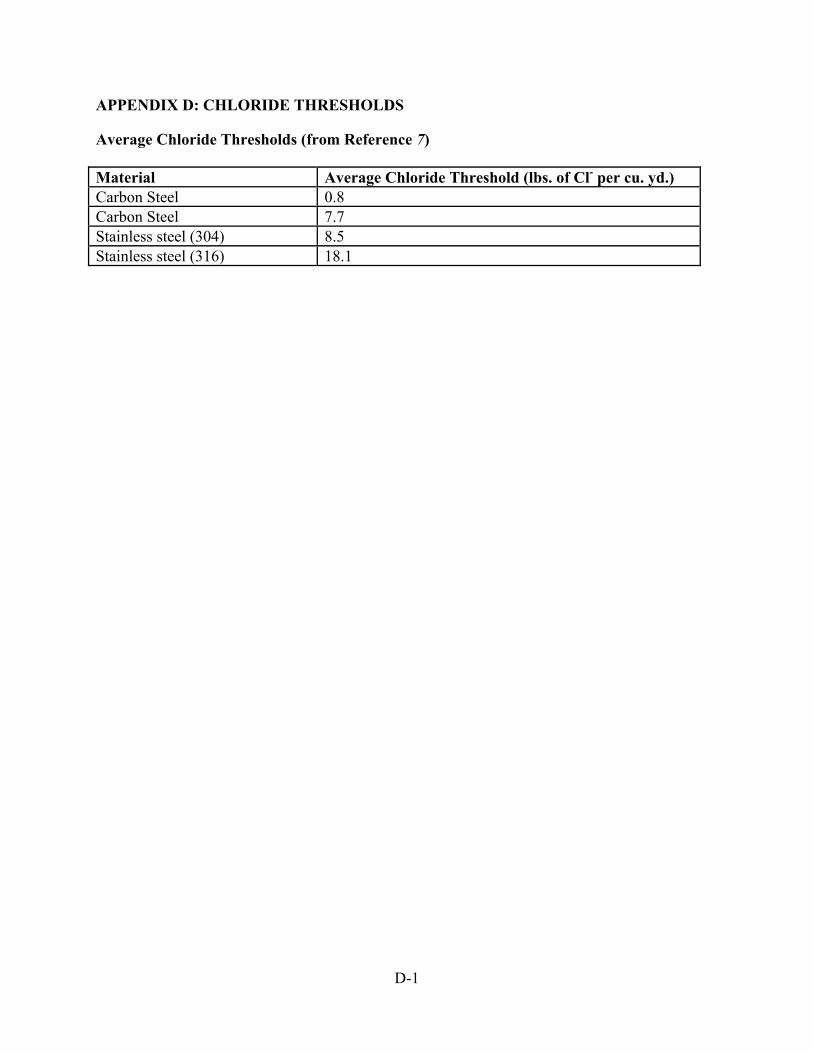
D-1
APPENDIX D: CHLORIDE THRESHOLDS
Average Chloride Thresholds (from Reference 7) Material Average Chloride Threshold (lbs. of Cl- per cu. yd.) Carbon Steel 0.8 Carbon Steel 7.7 Stainless steel (304) 8.5 Stainless steel (316) 18.1

D-2
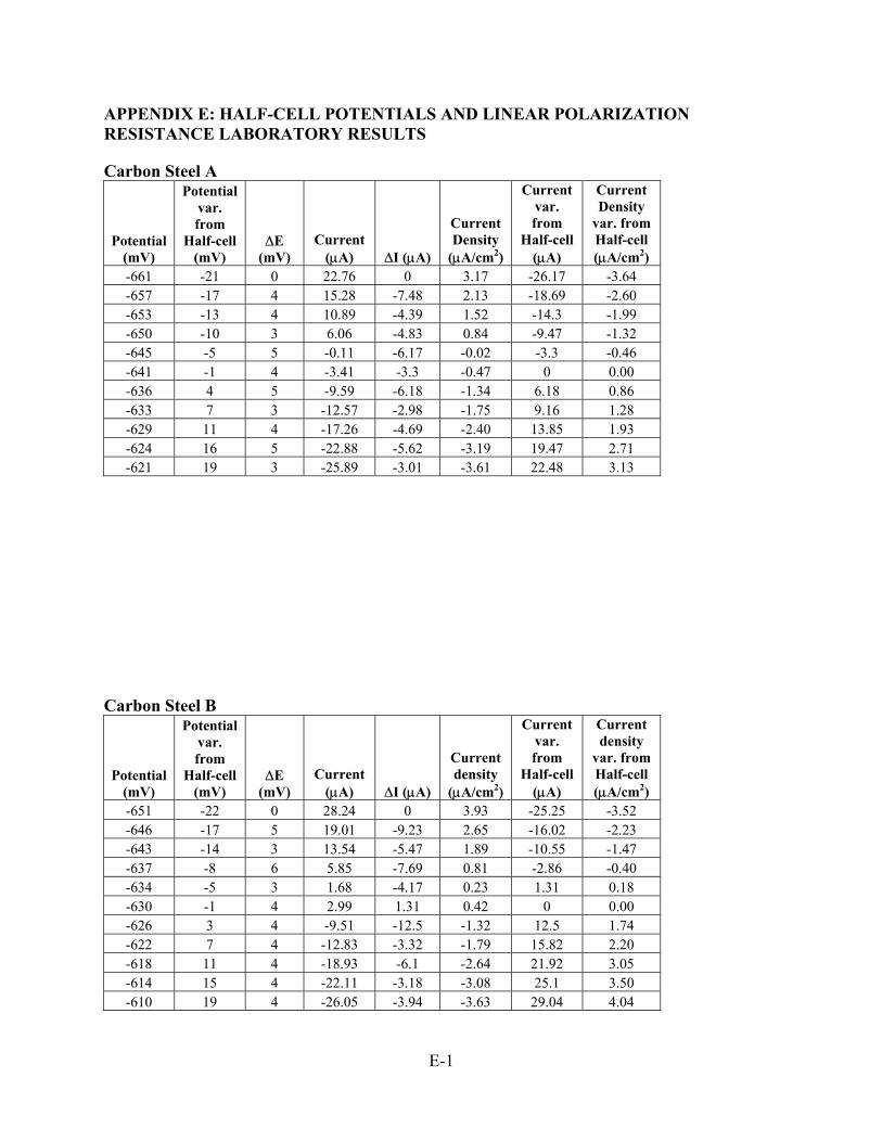
E-1
APPENDIX E: HALF-CELL POTENTIALS AND LINEAR POLARIZATION RESISTANCE LABORATORY RESULTS
Carbon Steel A
Potential (mV)
Potential var. from
Half-cell (mV)
∆E (mV)
Current (µA) ∆I (µA)
Current Density
(µA/cm2)
Current var. from
Half-cell (µA)
Current Density
var. from Half-cell (µA/cm2)
-661 -21 0 22.76 0 3.17 -26.17 -3.64 -657 -17 4 15.28 -7.48 2.13 -18.69 -2.60 -653 -13 4 10.89 -4.39 1.52 -14.3 -1.99 -650 -10 3 6.06 -4.83 0.84 -9.47 -1.32 -645 -5 5 -0.11 -6.17 -0.02 -3.3 -0.46 -641 -1 4 -3.41 -3.3 -0.47 0 0.00 -636 4 5 -9.59 -6.18 -1.34 6.18 0.86 -633 7 3 -12.57 -2.98 -1.75 9.16 1.28 -629 11 4 -17.26 -4.69 -2.40 13.85 1.93 -624 16 5 -22.88 -5.62 -3.19 19.47 2.71 -621 19 3 -25.89 -3.01 -3.61 22.48 3.13
Carbon Steel B
Potential (mV)
Potential var. from
Half-cell (mV)
∆E (mV)
Current (µA) ∆I (µA)
Current density
(µA/cm2)
Current var. from
Half-cell (µA)
Current density
var. from Half-cell (µA/cm2)
-651 -22 0 28.24 0 3.93 -25.25 -3.52 -646 -17 5 19.01 -9.23 2.65 -16.02 -2.23 -643 -14 3 13.54 -5.47 1.89 -10.55 -1.47 -637 -8 6 5.85 -7.69 0.81 -2.86 -0.40 -634 -5 3 1.68 -4.17 0.23 1.31 0.18 -630 -1 4 2.99 1.31 0.42 0 0.00 -626 3 4 -9.51 -12.5 -1.32 12.5 1.74 -622 7 4 -12.83 -3.32 -1.79 15.82 2.20 -618 11 4 -18.93 -6.1 -2.64 21.92 3.05 -614 15 4 -22.11 -3.18 -3.08 25.1 3.50 -610 19 4 -26.05 -3.94 -3.63 29.04 4.04

E-2
Carbon Steel C
Potential (mV)
Potential var. from
Half-cell (mV)
∆E (mV)
Current (µA) ∆I (µA)
Current density
(µA/cm2)
Current var. from
Half-cell (µA)
Current density
var. from Half-cell (µA/cm2)
-623 -21 0 46.81 0 6.52 -113.22 -15.77 -619 -17 4 18.78 -28.03 2.61 -85.19 -11.86 -614 -12 5 -11.41 -30.19 -1.59 -55 -7.66 -611 -9 3 -27.58 -16.17 -3.84 -38.83 -5.41 -607 -5 4 -52.25 -24.67 -7.28 -14.16 -1.97 -603 -1 4 -66.41 -14.16 -9.25 0 0.00 -599 3 4 -79.61 -13.2 -11.09 13.2 1.84 -595 7 4 -102.34 -22.73 -14.25 35.93 5.00 -591 11 4 -113.55 -11.21 -15.81 47.14 6.56 -587 15 4 -126.87 -13.32 -17.67 60.46 8.42 -583 19 4 -139.06 -12.19 -19.36 72.65 10.12
Carbon Steel D
Potential (mV)
Potential var. from
Half-cell (mV)
DE (mV)
Current (mA) ∆I (µA)
Current density
(µA/cm2)
Current var. from
Half-cell (µA)
Current density
var. from Half-cell (µA/cm2)
-714 -20 0 46.61 0 6.49 -64.06 -8.92 -711 -17 3 32.7 -13.91 4.55 -50.15 -6.98 -706 -12 5 15.12 -17.58 2.11 -32.57 -4.54 -703 -9 3 4.88 -10.24 0.68 -22.33 -3.11 -700 -6 3 3.79 -1.09 0.53 -21.24 -2.96 -695 -1 5 -17.45 -21.24 -2.43 0 0.00 -691 3 4 -25.36 -7.91 -3.53 7.91 1.10 -687 7 4 -38.24 -12.88 -5.32 20.79 2.89 -683 11 4 -44.64 -6.4 -6.22 27.19 3.79 -679 15 4 -53.69 -9.05 -7.48 36.24 5.05 -675 19 4 -65.02 -11.33 -9.05 47.57 6.62
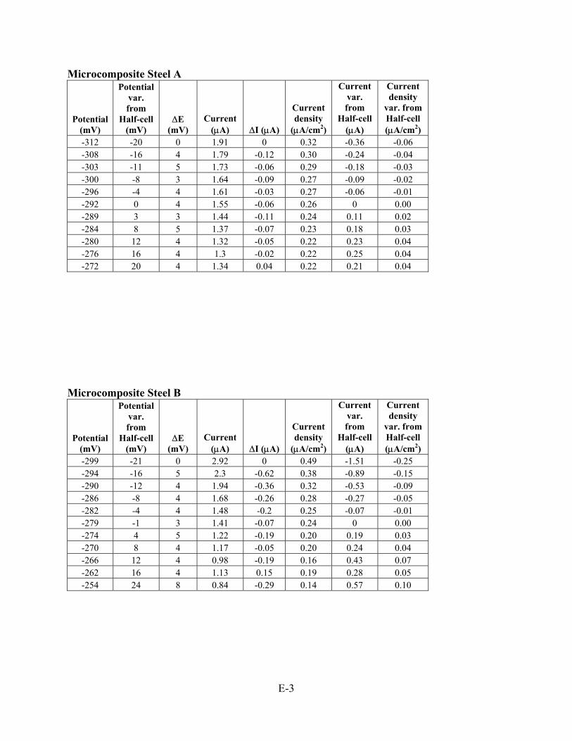
E-3
Microcomposite Steel A
Potential (mV)
Potential var. from
Half-cell (mV)
∆E (mV)
Current (µA) ∆I (µA)
Current density
(µA/cm2)
Current var. from
Half-cell (µA)
Current density
var. from Half-cell (µA/cm2)
-312 -20 0 1.91 0 0.32 -0.36 -0.06 -308 -16 4 1.79 -0.12 0.30 -0.24 -0.04 -303 -11 5 1.73 -0.06 0.29 -0.18 -0.03 -300 -8 3 1.64 -0.09 0.27 -0.09 -0.02 -296 -4 4 1.61 -0.03 0.27 -0.06 -0.01 -292 0 4 1.55 -0.06 0.26 0 0.00 -289 3 3 1.44 -0.11 0.24 0.11 0.02 -284 8 5 1.37 -0.07 0.23 0.18 0.03 -280 12 4 1.32 -0.05 0.22 0.23 0.04 -276 16 4 1.3 -0.02 0.22 0.25 0.04 -272 20 4 1.34 0.04 0.22 0.21 0.04
Microcomposite Steel B
Potential (mV)
Potential var. from
Half-cell (mV)
∆E (mV)
Current (µA) ∆I (µA)
Current density
(µA/cm2)
Current var. from
Half-cell (µA)
Current density
var. from Half-cell (µA/cm2)
-299 -21 0 2.92 0 0.49 -1.51 -0.25 -294 -16 5 2.3 -0.62 0.38 -0.89 -0.15 -290 -12 4 1.94 -0.36 0.32 -0.53 -0.09 -286 -8 4 1.68 -0.26 0.28 -0.27 -0.05 -282 -4 4 1.48 -0.2 0.25 -0.07 -0.01 -279 -1 3 1.41 -0.07 0.24 0 0.00 -274 4 5 1.22 -0.19 0.20 0.19 0.03 -270 8 4 1.17 -0.05 0.20 0.24 0.04 -266 12 4 0.98 -0.19 0.16 0.43 0.07 -262 16 4 1.13 0.15 0.19 0.28 0.05 -254 24 8 0.84 -0.29 0.14 0.57 0.10

E-4
Microcomposite Steel C
Potential (mV)
Potential var. from
Half-cell (mV)
∆E (mV)
Current (µA) ∆I (µA)
Current density
(µA/cm2)
Current var. from
Half-cell (µA)
Current density
var. from Half-cell (µA/cm2)
-592 -21 0 7.59 0 1.27 -7.14 -1.19 -588 -17 4 5.01 -2.58 0.84 -4.56 -0.76 -584 -13 4 3.73 -1.28 0.62 -3.28 -0.55 -580 -9 4 2.5 -1.23 0.42 -2.05 -0.34 -575 -4 5 1.19 -1.31 0.20 -0.74 -0.12 -572 -1 3 0.45 -0.74 0.08 0 0.00 -567 4 5 -0.5 -0.95 -0.08 0.95 0.16 -564 7 3 -1.14 -0.64 -0.19 1.59 0.27 -560 11 4 -1.77 -0.63 -0.30 2.22 0.37 -555 16 5 -2.71 -0.94 -0.45 3.16 0.53 -552 19 3 -3.18 -0.47 -0.53 3.63 0.61
Microcomposite Steel F
Potential (mV)
Potential var. from
Half-cell (mV)
∆E (mV)
Current (µA) ∆I (µA)
Current density
(µA/cm2)
Current var. from
Half-cell (µA)
Current density
var. from Half-cell (µA/cm2)
-587 -20 0 4.88 0 0.82 -7.05 -1.18 -584 -17 3 2.86 -2.02 0.48 -5.03 -0.84 -580 -13 4 1.32 -1.54 0.22 -3.49 -0.58 -575 -8 5 -0.3 -1.62 -0.05 -1.87 -0.31 -572 -5 3 -0.96 -0.66 -0.16 -1.21 -0.20 -567 0 5 -2.17 -1.21 -0.36 0 0.00 -564 3 3 -2.58 -0.41 -0.43 0.41 0.07 -560 7 4 -3.33 -0.75 -0.56 1.16 0.19 -555 12 5 -4.43 -1.1 -0.74 2.26 0.38 -552 15 3 -4.68 -0.25 -0.78 2.51 0.42 -547 20 5 -5.62 -0.94 -0.94 3.45 0.58

E-5
Stainless Steel Clad A
Potential (mV)
Potential var. from
Half-cell (mV)
∆E (mV)
Current (µA) ∆I (µA)
Current density
(µA/cm2)
Current var. from
Half-cell (µA)
Current density
var. from Half-cell (µA/cm2)
-235 -19 0 1.94 0 0.27 -0.52 -0.07 -232 -16 3 1.78 -0.16 0.25 -0.36 -0.05 -228 -12 4 1.7 -0.08 0.24 -0.28 -0.04 -223 -7 5 1.57 -0.13 0.22 -0.15 -0.02 -220 -4 3 1.54 -0.03 0.21 -0.12 -0.02 -215 1 5 1.42 -0.12 0.20 0 0.00 -212 4 3 1.39 -0.03 0.19 0.03 0.00 -208 8 4 1.31 -0.08 0.18 0.11 0.02 -203 13 5 1.15 -0.16 0.16 0.27 0.04 -200 16 3 1.19 0.04 0.17 0.23 0.03 -195 21 5 1.29 0.1 0.18 0.13 0.02
Stainless Steel Clad B
Potential (mV)
Potential var. from
Half-cell (mV)
∆E (mV)
Current (µA) ∆I (µA)
Current density
(µA/cm2)
Current var. from
Half-cell (µA)
Current density
var. from Half-cell (µA/cm2)
-299 -20 0 1.72 0 0.24 -0.7 -0.10 -294 -15 5 1.59 -0.13 0.22 -0.57 -0.08 -291 -12 3 1.37 -0.22 0.19 -0.35 -0.05 -287 -8 4 1.19 -0.18 0.17 -0.17 -0.02 -283 -4 4 1.1 -0.09 0.15 -0.08 -0.01 -279 0 4 1.02 -0.08 0.14 0 0.00 -274 5 5 0.5 -0.52 0.07 0.52 0.07 -271 8 3 1.04 0.54 0.14 -0.02 0.00 -266 13 5 0.53 -0.51 0.07 0.49 0.07 -263 16 3 0.93 0.4 0.13 0.09 0.01 -259 20 4 1.03 0.1 0.14 -0.01 0.00

E-6
Stainless Steel Clad B(2)
Potential (mV)
Potential var. from
Half-cell (mV)
∆E (mV)
Current (µA) ∆I (µA)
Current density
(µA/cm2)
Current var. from
Half-cell (µA)
Current density
var. from Half-cell (µA/cm2)
-305 -19 0 1.55 0 0.22 -0.68 -0.09 -302 -16 3 1.43 -0.12 0.20 -0.56 -0.08 -296 -10 6 1.26 -0.17 0.18 -0.39 -0.05 -293 -7 3 1.1 -0.16 0.15 -0.23 -0.03 -289 -3 4 0.99 -0.11 0.14 -0.12 -0.02 -285 1 4 0.87 -0.12 0.12 0 0.00 -281 5 4 0.93 0.06 0.13 -0.06 -0.01 -276 10 5 0.78 -0.15 0.11 0.09 0.01 -273 13 3 0.73 -0.05 0.10 0.14 0.02 -269 17 4 0.72 -0.01 0.10 0.15 0.02 -264 22 5 0.67 -0.05 0.09 0.2 0.03
Stainless Steel Clad D
Potential (mV)
Potential var. from
Half-cell (mV)
∆E (mV)
Current (µA) ∆I (µA)
Current density
(µA/cm2)
Current var. from
Half-cell (µA)
Current density
var. from Half-cell (µA/cm2)
-199 -20 0 2.26 0 0.31 -0.95 -0.13 -194 -15 5 1.86 -0.4 0.26 -0.55 -0.08 -191 -12 3 1.74 -0.12 0.24 -0.43 -0.06 -186 -7 5 1.56 -0.18 0.22 -0.25 -0.03 -183 -4 3 1.53 -0.03 0.21 -0.22 -0.03 -179 0 4 1.31 -0.22 0.18 0 0.00 -174 5 5 1.3 -0.01 0.18 0.01 0.00 -171 8 3 1.28 -0.02 0.18 0.03 0.00 -166 13 5 1.29 0.01 0.18 0.02 0.00 -163 16 3 1.08 -0.21 0.15 0.23 0.03 -159 20 4 1.1 0.02 0.15 0.21 0.03
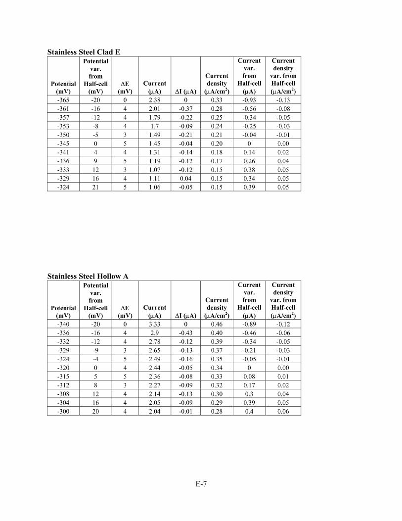
E-7
Stainless Steel Clad E
Potential (mV)
Potential var. from
Half-cell (mV)
∆E (mV)
Current (µA) ∆I (µA)
Current density
(µA/cm2)
Current var. from
Half-cell (µA)
Current density
var. from Half-cell (µA/cm2)
-365 -20 0 2.38 0 0.33 -0.93 -0.13 -361 -16 4 2.01 -0.37 0.28 -0.56 -0.08 -357 -12 4 1.79 -0.22 0.25 -0.34 -0.05 -353 -8 4 1.7 -0.09 0.24 -0.25 -0.03 -350 -5 3 1.49 -0.21 0.21 -0.04 -0.01 -345 0 5 1.45 -0.04 0.20 0 0.00 -341 4 4 1.31 -0.14 0.18 0.14 0.02 -336 9 5 1.19 -0.12 0.17 0.26 0.04 -333 12 3 1.07 -0.12 0.15 0.38 0.05 -329 16 4 1.11 0.04 0.15 0.34 0.05 -324 21 5 1.06 -0.05 0.15 0.39 0.05
Stainless Steel Hollow A
Potential (mV)
Potential var. from
Half-cell (mV)
∆E (mV)
Current (µA) ∆I (µA)
Current density
(µA/cm2)
Current var. from
Half-cell (µA)
Current density
var. from Half-cell (µA/cm2)
-340 -20 0 3.33 0 0.46 -0.89 -0.12 -336 -16 4 2.9 -0.43 0.40 -0.46 -0.06 -332 -12 4 2.78 -0.12 0.39 -0.34 -0.05 -329 -9 3 2.65 -0.13 0.37 -0.21 -0.03 -324 -4 5 2.49 -0.16 0.35 -0.05 -0.01 -320 0 4 2.44 -0.05 0.34 0 0.00 -315 5 5 2.36 -0.08 0.33 0.08 0.01 -312 8 3 2.27 -0.09 0.32 0.17 0.02 -308 12 4 2.14 -0.13 0.30 0.3 0.04 -304 16 4 2.05 -0.09 0.29 0.39 0.05 -300 20 4 2.04 -0.01 0.28 0.4 0.06

E-8
Stainless Steel Hollow B
Potential (mV)
Potential var. from
Half-cell (mV)
∆E (mV)
Current (µA) ∆I (µA)
Current density
(µA/cm2)
Current var. from
Half-cell (µA)
Current density
var. from Half-cell (µA/cm2)
-590 -21 0 2.28 0 0.32 -0.91 -0.13 -585 -16 5 1.95 -0.33 0.27 -0.58 -0.08 -582 -13 3 1.76 -0.19 0.25 -0.39 -0.05 -577 -8 5 1.61 -0.15 0.22 -0.24 -0.03 -574 -5 3 1.44 -0.17 0.20 -0.07 -0.01 -570 -1 4 1.37 -0.07 0.19 0 0.00 -565 4 5 1.23 -0.14 0.17 0.14 0.02 -562 7 3 1.11 -0.12 0.15 0.26 0.04 -557 12 5 0.88 -0.23 0.12 0.49 0.07 -554 15 3 0.83 -0.05 0.12 0.54 0.08 -550 19 4 0.76 -0.07 0.11 0.61 0.08
Stainless Steel Hollow D
Potential (mV)
Potential var. from
Half-cell (mV)
∆E (mV)
Current (µA) ∆I (µA)
Current density
(µA/cm2)
Current var. from
Half-cell (µA)
Current density
var. from Half-cell (µA/cm2)
-230 -20 0 2.07 0 0.29 -0.87 -0.12 -225 -15 5 1.62 -0.45 0.23 -0.42 -0.06 -222 -12 3 1.56 -0.06 0.22 -0.36 -0.05 -218 -8 4 1.4 -0.16 0.19 -0.2 -0.03 -213 -3 5 1.12 -0.28 0.16 0.08 0.01 -210 0 3 1.2 0.08 0.17 0 0.00 -205 5 5 1.01 -0.19 0.14 0.19 0.03 -202 8 3 0.89 -0.12 0.12 0.31 0.04 -198 12 4 1 0.11 0.14 0.2 0.03 -193 17 5 0.87 -0.13 0.12 0.33 0.05 -190 20 3 1.02 0.15 0.14 0.18 0.03

E-9
Stainless Steel Hollow F
Potential (mV)
Potential var. from
Half-cell (mV)
∆E (mV)
Current (µA) ∆I (µA)
Current density
(µA/cm2)
Current var. from
Half-cell (µA)
Current density
var. from Half-cell (µA/cm2)
-213 -20 0 1.94 0 0.27 -0.45 -0.06 -209 -16 4 1.8 -0.14 0.25 -0.31 -0.04 -204 -11 5 1.7 -0.1 0.24 -0.21 -0.03 -201 -8 3 1.59 -0.11 0.22 -0.1 -0.01 -196 -3 5 1.52 -0.07 0.21 -0.03 0.00 -193 0 3 1.49 -0.03 0.21 0 0.00 -189 4 4 1.51 0.02 0.21 -0.02 0.00 -184 9 5 1.45 -0.06 0.20 0.04 0.01 -181 12 3 1.45 0 0.20 0.04 0.01 -176 17 5 1.34 -0.11 0.19 0.15 0.02 -173 20 3 1.33 -0.01 0.19 0.16 0.02
Purple Non-flexible Epoxy A
Potential (mV)
Potential var. from
Half-cell (mV)
∆E (mV)
Current (µA) ∆I (µA)
Current density
(µA/cm2)
Current var. from
Half-cell (µA)
Current density
var. from Half-cell (µA/cm2)
-484 -20 0 1.55 0 0.22 -0.13 -0.02 -480 -16 4 1.52 -0.03 0.21 -0.1 -0.01 -476 -12 4 1.49 -0.03 0.21 -0.07 -0.01 -473 -9 3 1.47 -0.02 0.20 -0.05 -0.01 -469 -5 4 1.59 0.12 0.22 -0.17 -0.02 -464 0 5 1.42 -0.17 0.20 0 0.00 -461 3 3 1.45 0.03 0.20 -0.03 0.00 -456 8 5 1.5 0.05 0.21 -0.08 -0.01 -453 11 3 1.46 -0.04 0.20 -0.04 -0.01 -449 15 4 1.47 0.01 0.20 -0.05 -0.01 -444 20 5 1.52 0.05 0.21 -0.1 -0.01
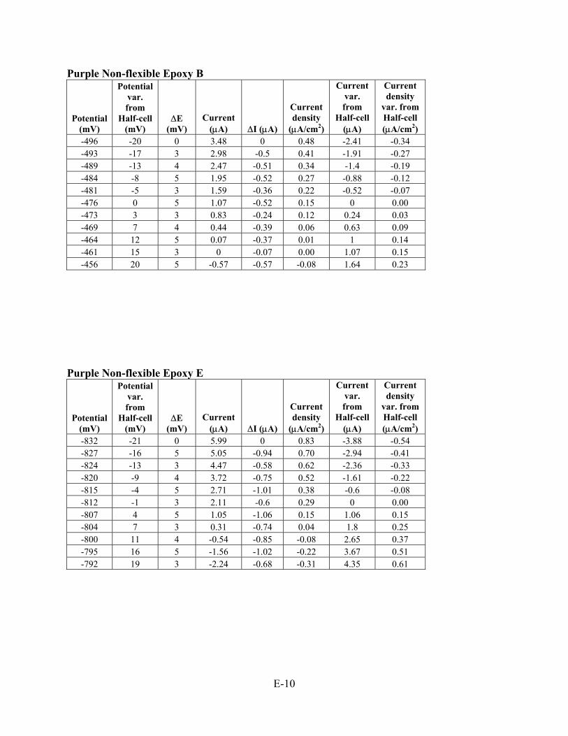
E-10
Purple Non-flexible Epoxy B
Potential (mV)
Potential var. from
Half-cell (mV)
∆E (mV)
Current (µA) ∆I (µA)
Current density
(µA/cm2)
Current var. from
Half-cell (µA)
Current density
var. from Half-cell (µA/cm2)
-496 -20 0 3.48 0 0.48 -2.41 -0.34 -493 -17 3 2.98 -0.5 0.41 -1.91 -0.27 -489 -13 4 2.47 -0.51 0.34 -1.4 -0.19 -484 -8 5 1.95 -0.52 0.27 -0.88 -0.12 -481 -5 3 1.59 -0.36 0.22 -0.52 -0.07 -476 0 5 1.07 -0.52 0.15 0 0.00 -473 3 3 0.83 -0.24 0.12 0.24 0.03 -469 7 4 0.44 -0.39 0.06 0.63 0.09 -464 12 5 0.07 -0.37 0.01 1 0.14 -461 15 3 0 -0.07 0.00 1.07 0.15 -456 20 5 -0.57 -0.57 -0.08 1.64 0.23
Purple Non-flexible Epoxy E
Potential (mV)
Potential var. from
Half-cell (mV)
∆E (mV)
Current (µA) ∆I (µA)
Current density
(µA/cm2)
Current var. from
Half-cell (µA)
Current density
var. from Half-cell (µA/cm2)
-832 -21 0 5.99 0 0.83 -3.88 -0.54 -827 -16 5 5.05 -0.94 0.70 -2.94 -0.41 -824 -13 3 4.47 -0.58 0.62 -2.36 -0.33 -820 -9 4 3.72 -0.75 0.52 -1.61 -0.22 -815 -4 5 2.71 -1.01 0.38 -0.6 -0.08 -812 -1 3 2.11 -0.6 0.29 0 0.00 -807 4 5 1.05 -1.06 0.15 1.06 0.15 -804 7 3 0.31 -0.74 0.04 1.8 0.25 -800 11 4 -0.54 -0.85 -0.08 2.65 0.37 -795 16 5 -1.56 -1.02 -0.22 3.67 0.51 -792 19 3 -2.24 -0.68 -0.31 4.35 0.61

E-11
Purple Non-flexible Epoxy F
Potential (mV)
Potential var. from
Half-cell (mV)
∆E (mV)
Current (µA) ∆I (µA)
Current density
(µA/cm2)
Current var. from
Half-cell (µA)
Current density
var. from Half-cell (µA/cm2)
-603 -21 0 1.77 0 0.25 -0.16 -0.02 -599 -17 4 1.75 -0.02 0.24 -0.14 -0.02 -595 -13 4 1.7 -0.05 0.24 -0.09 -0.01 -591 -9 4 1.68 -0.02 0.23 -0.07 -0.01 -587 -5 4 1.62 -0.06 0.23 -0.01 0.00 -583 -1 4 1.61 -0.01 0.22 0 0.00 -579 3 4 1.59 -0.02 0.22 0.02 0.00 -574 8 5 1.59 0 0.22 0.02 0.00 -571 11 3 1.48 -0.11 0.21 0.13 0.02 -567 15 4 1.57 0.09 0.22 0.04 0.01 -563 19 4 1.53 -0.04 0.21 0.08 0.01
Gray Non-flexible Epoxy A
Potential (mV)
Potential var. from
Half-cell (mV)
∆E (mV)
Current (µA) ∆I (µA)
Current density
(µA/cm2)
Current var. from
Half-cell (µA)
Current density
var. from Half-cell (µA/cm2)
-617 -20 0 1.46 0 0.20 -0.01 0.00 -614 -17 3 1.61 0.15 0.22 -0.16 -0.02 -609 -12 5 1.5 -0.11 0.21 -0.05 -0.01 -605 -8 4 1.47 -0.03 0.20 -0.02 0.00 -602 -5 3 1.54 0.07 0.21 -0.09 -0.01 -597 0 5 1.45 -0.09 0.20 0 0.00 -594 3 3 1.54 0.09 0.21 -0.09 -0.01 -590 7 4 1.49 -0.05 0.21 -0.04 -0.01 -585 12 5 1.54 0.05 0.21 -0.09 -0.01 -582 15 3 1.49 -0.05 0.21 -0.04 -0.01 -577 20 5 1.48 -0.01 0.21 -0.03 0.00

E-12
Gray Non-flexible Epoxy B
Potential (mV)
Potential var. from
Half-cell (mV)
∆E (mV)
Current (µA) ∆I (µA)
Current density
(µA/cm2)
Current var. from
Half-cell (µA)
Current density
var. from Half-cell (µA/cm2)
-425 -20 0 1.57 0 0.22 -0.01 0.00 -421 -16 4 1.55 -0.02 0.22 0.01 0.00 -417 -12 4 1.56 0.01 0.22 0 0.00 -413 -8 4 1.53 -0.03 0.21 0.03 0.00 -410 -5 3 1.49 -0.04 0.21 0.07 0.01 -405 0 5 1.56 0.07 0.22 0 0.00 -401 4 4 1.41 -0.15 0.20 0.15 0.02 -397 8 4 1.61 0.2 0.22 -0.05 -0.01 -393 12 4 1.5 -0.11 0.21 0.06 0.01 -390 15 3 1.46 -0.04 0.20 0.1 0.01 -385 20 5 1.35 -0.11 0.19 0.21 0.03
Gray Non-flexible Epoxy C
Potential (mV)
Potential var. from
Half-cell (mV)
∆E (mV)
Current (µA) ∆I (µA)
Current density
(µA/cm2)
Current var. from
Half-cell (µA)
Current density
var. from Half-cell (µA/cm2)
-651 -21 0 1.39 0 0.19 -0.14 -0.02 -646 -16 5 1.39 0 0.19 -0.14 -0.02 -643 -13 3 1.28 -0.11 0.18 -0.03 0.00 -639 -9 4 1.29 0.01 0.18 -0.04 -0.01 -634 -4 5 1.19 -0.1 0.17 0.06 0.01 -631 -1 3 1.25 0.06 0.17 0 0.00 -626 4 5 1.13 -0.12 0.16 0.12 0.02 -623 7 3 1.14 0.01 0.16 0.11 0.02 -619 11 4 1.15 0.01 0.16 0.1 0.01 -614 16 5 1.07 -0.08 0.15 0.18 0.03 -610 20 4 1.04 -0.03 0.14 0.21 0.03

E-13
Gray Non-flexible Epoxy D
Potential (mV)
Potential var. from
Half-cell (mV)
∆E (mV)
Current (µA) ∆I (µA)
Current density
(µA/cm2)
Current var. from
Half-cell (µA)
Current density
var. from Half-cell (µA/cm2)
-670 -22 0 3.12 0 0.43 -1.7 -0.24 -665 -17 5 2.56 -0.56 0.36 -1.14 -0.16 -662 -14 3 2.22 -0.34 0.31 -0.8 -0.11 -657 -9 5 1.82 -0.4 0.25 -0.4 -0.06 -653 -5 4 1.65 -0.17 0.23 -0.23 -0.03 -650 -2 3 1.42 -0.23 0.20 0 0.00 -645 3 5 1.12 -0.3 0.16 0.3 0.04 -642 6 3 0.95 -0.17 0.13 0.47 0.07 -639 9 3 0.96 0.01 0.13 0.46 0.06 -635 13 4 0.66 -0.3 0.09 0.76 0.11 -631 17 4 0.38 -0.28 0.05 1.04 0.14
Green Flexible Epoxy B
Potential (mV)
Potential var. from
Half-cell (mV)
∆E (mV)
Current (µA) ∆I (µA)
Current density
(µA/cm2)
Current var. from
Half-cell (µA)
Current density
var. from Half-cell (µA/cm2)
-782 -22 0 3.06 0 0.43 -1.74 -0.24 -777 -17 5 2.47 -0.59 0.34 -1.15 -0.16 -774 -14 3 2.11 -0.36 0.29 -0.79 -0.11 -770 -10 4 1.89 -0.22 0.26 -0.57 -0.08 -765 -5 5 1.56 -0.33 0.22 -0.24 -0.03 -762 -2 3 1.32 -0.24 0.18 0 0.00 -757 3 5 1.21 -0.11 0.17 0.11 0.02 -754 6 3 1.17 -0.04 0.16 0.15 0.02 -750 10 4 0.94 -0.23 0.13 0.38 0.05 -745 15 5 0.73 -0.21 0.10 0.59 0.08 -742 18 3 0.54 -0.19 0.08 0.78 0.11

E-14
Green Flexible Epoxy C
Potential (mV)
Potential var. from
Half-cell (mV)
∆E (mV)
Current (µA) ∆I (µA)
Current density
(µA/cm2)
Current var. from
Half-cell (µA)
Current density
var. from Half-cell (µA/cm2)
-665 -22 0 1.78 0 0.25 -0.12 -0.02 -661 -18 4 1.75 -0.03 0.24 -0.09 -0.01 -656 -13 5 1.73 -0.02 0.24 -0.07 -0.01 -653 -10 3 1.66 -0.07 0.23 0 0.00 -648 -5 5 1.69 0.03 0.24 -0.03 0.00 -645 -2 3 1.66 -0.03 0.23 0 0.00 -641 2 4 1.69 0.03 0.24 -0.03 0.00 -636 7 5 1.59 -0.1 0.22 0.07 0.01 -632 11 4 1.55 -0.04 0.22 0.11 0.02 -628 15 4 1.56 0.01 0.22 0.1 0.01 -624 19 4 1.54 -0.02 0.21 0.12 0.02
Green Flexible Epoxy D
Potential (mV)
Potential var. from
Half-cell (mV)
∆E (mV)
Current (µA) ∆I (µA)
Current density
(µA/cm2)
Current var. from
Half-cell (µA)
Current density
var. from Half-cell (µA/cm2)
-440 -20 0 1.16 0 0.16 -0.04 -0.01 -435 -15 5 1.08 -0.08 0.15 0.04 0.01 -432 -12 3 1.07 -0.01 0.15 0.05 0.01 -428 -8 4 1.1 0.03 0.15 0.02 0.00 -423 -3 5 1.15 0.05 0.16 -0.03 0.00 -420 0 3 1.12 -0.03 0.16 0 0.00 -415 5 5 1.11 -0.01 0.15 0.01 0.00 -412 8 3 1.22 0.11 0.17 -0.1 -0.01 -406 14 6 1.09 -0.13 0.15 0.03 0.00 -403 17 3 1.06 -0.03 0.15 0.06 0.01 -400 20 3 1.12 0.06 0.16 0 0.00

E-15
Green Flexible Epoxy E
Potential (mV)
Potential var. from
Half-cell (mV)
∆E (mV)
Current (µA) ∆I (µA)
Current density
(µA/cm2)
Current var. from
Half-cell (µA)
Current density
var. from Half-cell (µA/cm2)
-579 -21 0 1.69 0 0.24 -0.16 -0.02 -574 -16 5 1.77 0.08 0.25 -0.24 -0.03 -571 -13 3 1.56 -0.21 0.22 -0.03 0.00 -566 -8 5 1.51 -0.05 0.21 0.02 0.00 -563 -5 3 1.54 0.03 0.21 -0.01 0.00 -559 -1 4 1.53 -0.01 0.21 0 0.00 -554 4 5 1.53 0 0.21 0 0.00 -551 7 3 1.54 0.01 0.21 -0.01 0.00 -547 11 4 1.57 0.03 0.22 -0.04 -0.01 -543 15 4 1.55 -0.02 0.22 -0.02 0.00 -539 19 4 1.55 0 0.22 -0.02 0.00

E-16

F-1
APPENDIX F: CHLORIDE TEST RESULTS
WSDOT Slab Core 1
Sample Depth (x) Depth (in.) Chloride (mg/kg) Chloride (mass%) kg/m3 lb./cu. yd. C1-1 4 0.16 1700 0.170 4.3 7.16 C1-2 8 0.31 3500 0.350 8.8 14.75 C1-3 12 0.47 3500 0.350 8.8 14.75 C1-4 16 0.63 3100 0.310 7.8 13.06 C1-5 20 0.79 2100 0.210 5.3 8.85 C1-6 24 0.94 2200 0.220 5.5 9.27 C1-7 28 1.10 1700 0.170 4.3 7.16 C1-8 32 1.26 1500 0.150 3.8 6.32 C1-9 36 1.42 1400 0.140 3.5 5.90 C1-10 40 1.57 1000 0.100 2.5 4.21 C1-11 44 1.73 1100 0.110 2.8 4.64 C1-12 48 1.89 740 0.074 1.9 3.12 C1-13 52 2.05 700 0.070 1.8 2.95 C1-14 56 2.20 630 0.063 1.6 2.65 C1-15 60 2.36 410 0.041 1.0 1.73 C1-BG 70 2.76 170 0.017 0.4 0.72
WSDOT Slab Core 2
Sample Depth (x) Depth (in.) Chloride (mg/kg) Chloride (mass%) kg/m3 lb./cu. yd. C2-1 4 0.16 1200 0.120 3.0 5.06 C2-2 8 0.31 3500 0.350 8.8 14.75 C2-3 12 0.47 3300 0.330 8.3 13.91 C2-4 16 0.63 2900 0.290 7.3 12.22 C2-5 20 0.79 2800 0.280 7.0 11.80 C2-6 24 0.94 2400 0.240 6.0 10.11 C2-7 28 1.10 2300 0.230 5.8 9.69 C2-8 32 1.26 2100 0.210 5.3 8.85 C2-9 36 1.42 1600 0.160 4.0 6.74 C2-10 40 1.57 1000 0.100 2.5 4.21 C2-11 44 1.73 790 0.079 2.0 3.33 C2-12 48 1.89 850 0.085 2.1 3.58 C2-13 52 2.05 610 0.061 1.5 2.57 C2-14 56 2.20 380 0.038 1.0 1.60 C2-15 60 2.36 410 0.041 1.0 1.73 C2-16 64 2.52 330 0.033 0.8 1.39 C2-17 68 2.68 300 0.030 0.8 1.26 C2-BG 75 2.95 250 0.025 0.6 1.05

F-2
WSDOT Slab Core 3
Sample Depth (x) Depth (in.) Chloride (mg/kg) Chloride (mass%) kg/m3 lb./cu. yd. C3-1 4 0.16 1600 0.160 4.0 6.74 C3-2 8 0.31 1000 0.100 2.5 4.21 C3-3 12 0.47 650 0.065 1.6 2.74 C3-4 16 0.63 440 0.044 1.1 1.85 C3-5 20 0.79 280 0.028 0.7 1.18 C3-6 24 0.94 250 0.025 0.6 1.05 C3-7 28 1.10 160 0.016 0.4 0.67 C3-8 32 1.26 150 0.015 0.4 0.63 C3-9 36 1.42 130 0.013 0.3 0.55 C3-10 40 1.57 85 0.009 0.2 0.36 C3-11 44 1.73 170 0.017 0.4 0.72 C3-12 48 1.89 81 0.008 0.2 0.34 C3-13 52 2.05 59 0.006 0.1 0.25 C3-14 56 2.20 35 0.004 0.1 0.15 C3-BG 70 2.76 10 0.001 0.0 0.04
WSDOT Slab Core 5
Sample Depth (x) Depth (in.) Chloride (mg/kg) Chloride (mass%) kg/m3 lb./cu. yd. C5-A2 4 0.16 2300 0.23 5.8 9.69 C5-A3 8 0.31 2100 0.21 5.3 8.85 C5-A4 12 0.47 1900 0.19 4.8 8.01 C5-A5 16 0.63 1700 0.17 4.3 7.16 C5-A6 20 0.79 1800 0.18 4.5 7.58 C5-A7 24 0.94 1900 0.19 4.8 8.01 C5-A8 28 1.10 1900 0.19 4.8 8.01 C5-A9 32 1.26 2000 0.2 5.0 8.43 C5-A10 36 1.42 1500 0.15 3.8 6.32 C5-ADB 40 1.57 660 0.066 1.7 2.78 C5-ABG1 44 1.73 260 0.026 0.7 1.10 C5-ABG2 70 2.76 18 0.0018 0.0
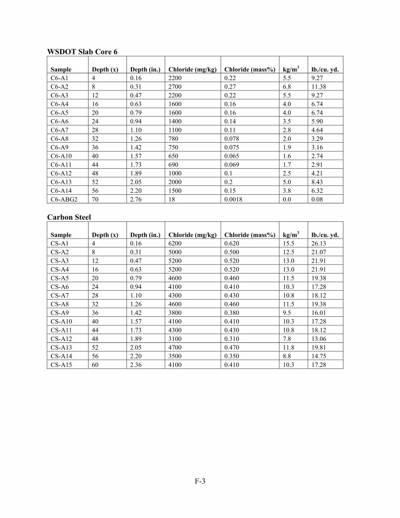
F-3
WSDOT Slab Core 6
Sample Depth (x) Depth (in.) Chloride (mg/kg) Chloride (mass%) kg/m3 lb./cu. yd. C6-A1 4 0.16 2200 0.22 5.5 9.27 C6-A2 8 0.31 2700 0.27 6.8 11.38 C6-A3 12 0.47 2200 0.22 5.5 9.27 C6-A4 16 0.63 1600 0.16 4.0 6.74 C6-A5 20 0.79 1600 0.16 4.0 6.74 C6-A6 24 0.94 1400 0.14 3.5 5.90 C6-A7 28 1.10 1100 0.11 2.8 4.64 C6-A8 32 1.26 780 0.078 2.0 3.29 C6-A9 36 1.42 750 0.075 1.9 3.16 C6-A10 40 1.57 650 0.065 1.6 2.74 C6-A11 44 1.73 690 0.069 1.7 2.91 C6-A12 48 1.89 1000 0.1 2.5 4.21 C6-A13 52 2.05 2000 0.2 5.0 8.43 C6-A14 56 2.20 1500 0.15 3.8 6.32 C6-ABG2 70 2.76 18 0.0018 0.0 0.08
Carbon Steel
Sample Depth (x) Depth (in.) Chloride (mg/kg) Chloride (mass%) kg/m3 lb./cu. yd. CS-A1 4 0.16 6200 0.620 15.5 26.13 CS-A2 8 0.31 5000 0.500 12.5 21.07 CS-A3 12 0.47 5200 0.520 13.0 21.91 CS-A4 16 0.63 5200 0.520 13.0 21.91 CS-A5 20 0.79 4600 0.460 11.5 19.38 CS-A6 24 0.94 4100 0.410 10.3 17.28 CS-A7 28 1.10 4300 0.430 10.8 18.12 CS-A8 32 1.26 4600 0.460 11.5 19.38 CS-A9 36 1.42 3800 0.380 9.5 16.01 CS-A10 40 1.57 4100 0.410 10.3 17.28 CS-A11 44 1.73 4300 0.430 10.8 18.12 CS-A12 48 1.89 3100 0.310 7.8 13.06 CS-A13 52 2.05 4700 0.470 11.8 19.81 CS-A14 56 2.20 3500 0.350 8.8 14.75 CS-A15 60 2.36 4100 0.410 10.3 17.28
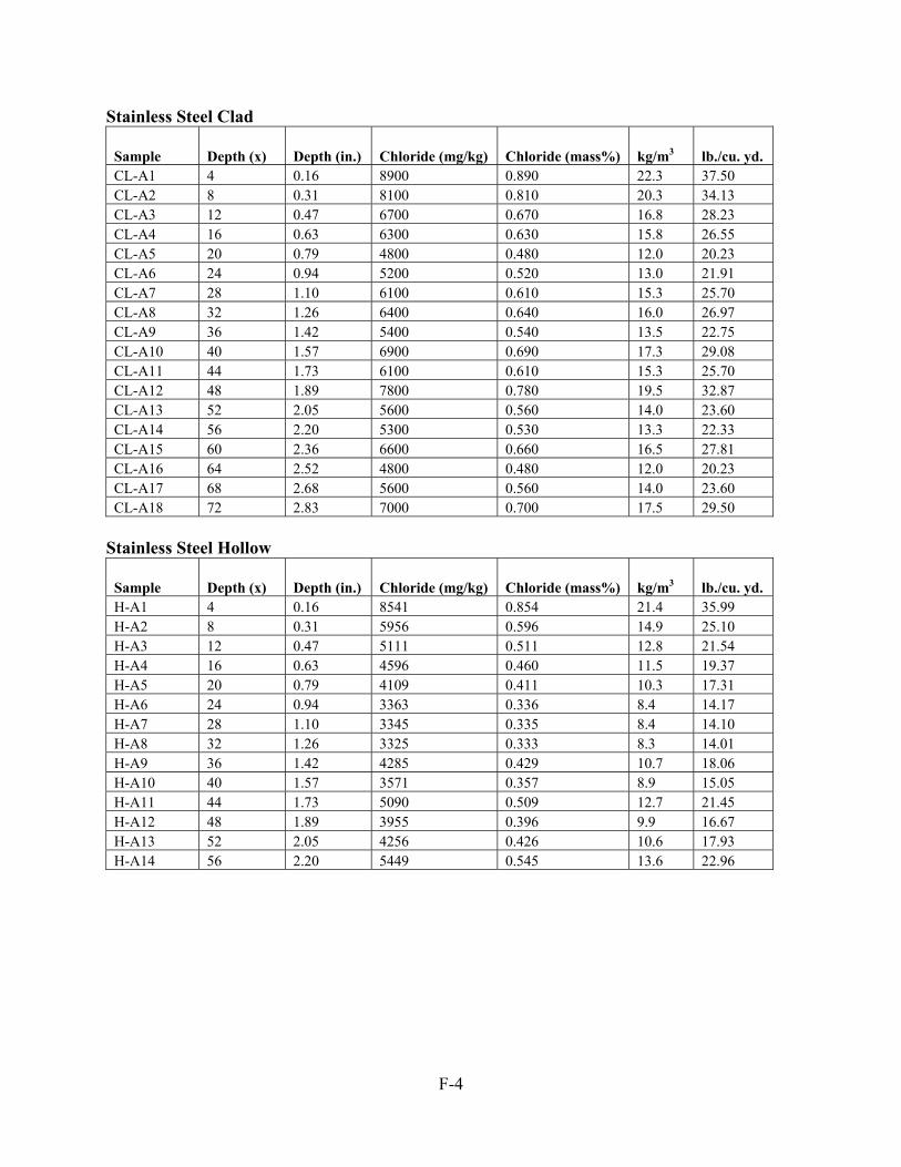
F-4
Stainless Steel Clad
Sample Depth (x) Depth (in.) Chloride (mg/kg) Chloride (mass%) kg/m3 lb./cu. yd. CL-A1 4 0.16 8900 0.890 22.3 37.50 CL-A2 8 0.31 8100 0.810 20.3 34.13 CL-A3 12 0.47 6700 0.670 16.8 28.23 CL-A4 16 0.63 6300 0.630 15.8 26.55 CL-A5 20 0.79 4800 0.480 12.0 20.23 CL-A6 24 0.94 5200 0.520 13.0 21.91 CL-A7 28 1.10 6100 0.610 15.3 25.70 CL-A8 32 1.26 6400 0.640 16.0 26.97 CL-A9 36 1.42 5400 0.540 13.5 22.75 CL-A10 40 1.57 6900 0.690 17.3 29.08 CL-A11 44 1.73 6100 0.610 15.3 25.70 CL-A12 48 1.89 7800 0.780 19.5 32.87 CL-A13 52 2.05 5600 0.560 14.0 23.60 CL-A14 56 2.20 5300 0.530 13.3 22.33 CL-A15 60 2.36 6600 0.660 16.5 27.81 CL-A16 64 2.52 4800 0.480 12.0 20.23 CL-A17 68 2.68 5600 0.560 14.0 23.60 CL-A18 72 2.83 7000 0.700 17.5 29.50
Stainless Steel Hollow
Sample Depth (x) Depth (in.) Chloride (mg/kg) Chloride (mass%) kg/m3 lb./cu. yd. H-A1 4 0.16 8541 0.854 21.4 35.99 H-A2 8 0.31 5956 0.596 14.9 25.10 H-A3 12 0.47 5111 0.511 12.8 21.54 H-A4 16 0.63 4596 0.460 11.5 19.37 H-A5 20 0.79 4109 0.411 10.3 17.31 H-A6 24 0.94 3363 0.336 8.4 14.17 H-A7 28 1.10 3345 0.335 8.4 14.10 H-A8 32 1.26 3325 0.333 8.3 14.01 H-A9 36 1.42 4285 0.429 10.7 18.06 H-A10 40 1.57 3571 0.357 8.9 15.05 H-A11 44 1.73 5090 0.509 12.7 21.45 H-A12 48 1.89 3955 0.396 9.9 16.67 H-A13 52 2.05 4256 0.426 10.6 17.93 H-A14 56 2.20 5449 0.545 13.6 22.96
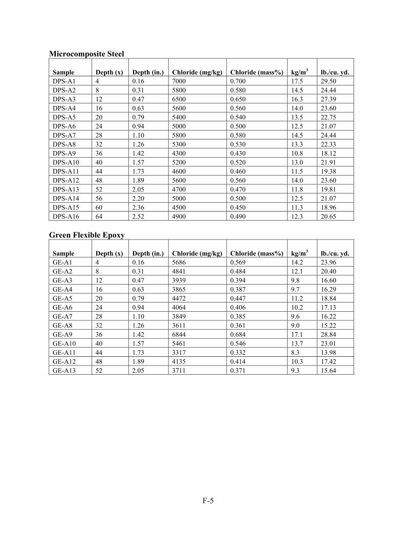
F-5
Microcomposite Steel
Sample Depth (x) Depth (in.) Chloride (mg/kg) Chloride (mass%) kg/m3 lb./cu. yd. DPS-A1 4 0.16 7000 0.700 17.5 29.50 DPS-A2 8 0.31 5800 0.580 14.5 24.44 DPS-A3 12 0.47 6500 0.650 16.3 27.39 DPS-A4 16 0.63 5600 0.560 14.0 23.60 DPS-A5 20 0.79 5400 0.540 13.5 22.75 DPS-A6 24 0.94 5000 0.500 12.5 21.07 DPS-A7 28 1.10 5800 0.580 14.5 24.44 DPS-A8 32 1.26 5300 0.530 13.3 22.33 DPS-A9 36 1.42 4300 0.430 10.8 18.12 DPS-A10 40 1.57 5200 0.520 13.0 21.91 DPS-A11 44 1.73 4600 0.460 11.5 19.38 DPS-A12 48 1.89 5600 0.560 14.0 23.60 DPS-A13 52 2.05 4700 0.470 11.8 19.81 DPS-A14 56 2.20 5000 0.500 12.5 21.07 DPS-A15 60 2.36 4500 0.450 11.3 18.96 DPS-A16 64 2.52 4900 0.490 12.3 20.65
Green Flexible Epoxy
Sample Depth (x) Depth (in.) Chloride (mg/kg) Chloride (mass%) kg/m3 lb./cu. yd. GE-A1 4 0.16 5686 0.569 14.2 23.96 GE-A2 8 0.31 4841 0.484 12.1 20.40 GE-A3 12 0.47 3939 0.394 9.8 16.60 GE-A4 16 0.63 3865 0.387 9.7 16.29 GE-A5 20 0.79 4472 0.447 11.2 18.84 GE-A6 24 0.94 4064 0.406 10.2 17.13 GE-A7 28 1.10 3849 0.385 9.6 16.22 GE-A8 32 1.26 3611 0.361 9.0 15.22 GE-A9 36 1.42 6844 0.684 17.1 28.84 GE-A10 40 1.57 5461 0.546 13.7 23.01 GE-A11 44 1.73 3317 0.332 8.3 13.98 GE-A12 48 1.89 4135 0.414 10.3 17.42 GE-A13 52 2.05 3711 0.371 9.3 15.64

F-6
Purple Non-flexible Epoxy
Sample Depth (x) Depth (in.) Chloride (mg/kg) Chloride (mass%) kg/m3 lb./cu. yd. E-A1 4 0.16 8600 0.860 21.5 36.24 E-A2 8 0.31 3500 0.350 8.8 14.75 E-A3 12 0.47 6100 0.610 15.3 25.70 E-A4 16 0.63 5800 0.580 14.5 24.44 E-A5 20 0.79 6300 0.630 15.8 26.55 E-A6 24 0.94 5400 0.540 13.5 22.75 E-A7 28 1.10 3500 0.350 8.8 14.75 E-A8 32 1.26 5600 0.560 14.0 23.60 E-A9 36 1.42 3500 0.350 8.8 14.75 E-A10 40 1.57 4900 0.490 12.3 20.65 E-A11 44 1.73 5300 0.530 13.3 22.33 E-A12 48 1.89 4600 0.460 11.5 19.38 E-A13 52 2.05 3500 0.350 8.8 14.75 E-A14 56 2.20 4200 0.420 10.5 17.70 E-A15 60 2.36 5200 0.520 13.0 21.91 E-A16 64 2.52 4800 0.480 12.0 20.23

G-1
APPENDIX G: CONCRETE TECHNOLOGY LABORATORIES (CTL) RESULTS (RAW DATA)

G-2

G-3

G-4

APPENDIX H: CHARACTERISTICS OF MICROCOMPOSITE STEEL USED IN THE RESEARCH
Information provided by manufacturer.
MMFX Heat info
Heat history:
MMFX # Grade Melting Plant Melt # Melt Date Size Roll Plant Roll# Roll Date Cert DateD-55A100 GR75 Nucor, NE 710789 12/11/2000 1 1/4" Nucor, NE 710789 1/20/2001 1/20/2001
Chemistry info:
C% Mn% Si% S% P% Cu% Cr% Ni% Mo% V% Nb% N2 ppm 0.06 0.43 0.29 0.008 0.01 0.1 9.28 0.08 0.02 0.018 0.007 110 Machined bars from 1 1/2" 710789 heat As rolled testing info:
MMFX # Testing Location and Date
Yield, [PSI]
Yield [MPa]
0.35% stress Mpa
Tensile [PSI]
Tensile Elongationin 8" [MPa] [%]
Bend Pass /Fail
D-55A100 Houston 4/2/2004 143600 990 756 183000 1262 16.05 P
D-55A100 Houston 4/2/2004 144100 994 621 177700 1225 13.19 P
H-1