Measuring the spatial resolution of an optical system in an undergraduate opticslaboratoryCalvin Leung and T. D. Donnelly

Citation: American Journal of Physics 85, 429 (2017); doi: 10.1119/1.4979539View online: http://dx.doi.org/10.1119/1.4979539View Table of Contents: http://aapt.scitation.org/toc/ajp/85/6Published by the American Association of Physics Teachers

Measuring the spatial resolution of an optical systemin an undergraduate optics laboratory

Calvin Leung and T. D. DonnellyDepartment of Physics, Harvey Mudd College, Claremont, 91711, USA

(Received 13 June 2016; accepted 12 February 2017)

Two methods of quantifying the spatial resolution of a camera are described, performed, and

compared, with the objective of designing an imaging-system experiment for students in an

undergraduate optics laboratory. With the goal of characterizing the resolution of a typical digital

single-lens reflex (DSLR) camera, we motivate, introduce, and show agreement between traditional

test-target contrast measurements and the technique of using Fourier analysis to obtain the

modulation transfer function (MTF). The advantages and drawbacks of each method are compared.

Finally, we explore the rich optical physics at work in the camera system by calculating the MTF

as a function of wavelength and f-number. For example, we find that the Canon 40D demonstrates

better spatial resolution at short wavelengths, in accordance with scalar diffraction theory, but is

not diffraction-limited, being significantly affected by spherical aberration. The experiment and

data analysis routines described here can be built and written in an undergraduate optics lab setting.VC 2017 American Association of Physics Teachers.

[http://dx.doi.org/10.1119/1.4979539]

I. INTRODUCTION

What is meant when we say a camera is high quality? Wemight mean that the camera can do justice to an unevenly litscene, or has a high dynamic range. Maybe the camera’s sen-sor has many pixels and thus round objects do not appearpixelated. Or perhaps we mean the camera responds consis-tently to different colors of light, or has very little chromaticaberration. Maybe we mean to say that the camera has goodspatial resolution, that it does a good job of reproducingsmall objects, sharp edges, and fine detail.

Spatial resolution measurements are a standard way to testthe quality of an optical system. Having a resolution-measurement testbed in an undergraduate optics lab is aninteresting and relevant way to learn about optics andelectro-optical systems. For the hobbyist, the curious student,or anybody with a smartphone camera, it is interesting andworthwhile to be able to quantitatively compare differentimaging options on the market. In particular, off-the-shelfDSLR cameras, such as the Canon 40D, are compelling sys-tems to study because they are ubiquitous, the technologicalbang-for-the-buck is very high, and there is a great deal ofconsumer interest in selecting appropriate cameras andlenses. In this paper, we explore two ways in which a cam-era’s spatial resolution can be measured and investigate thedependence of the resolution on various parameters of thecamera. A widely accepted method for quantifying the per-formance of imaging systems is through the use of a set ofresolution test targets. Another more sophisticated methoduses Fourier analysis and measures the camera’s response tothe different spatial-frequency components of a known sig-nal. Using the modulation transfer function to quantify reso-lution illustrates the power of using the discrete Fouriertransform as a robust tool to extract subtle patterns from spa-tial data.

In the remainder of this paper, we first motivate the studyof spatial resolution by discussing scalar diffraction theory,which predicts fundamental physical limits on the spatial res-olution of any imaging system. Then, we introduce theexperimental setup we will use and present procedures and

the necessary mathematical formalism for making measure-ments via both techniques. A set of measurements is madevia both of these methods. The data analysis procedures aredescribed in detail and the results are compared. Finally, asan application of this work, we characterize the Canon 40Dand perform two tests that confirm that it is not diffractionlimited.

There is a vast literature on spatial resolution, Fouriertransforms,1 and methods of quantifying optical systems,both in the peer-reviewed literature and in textbooks.2 Theimportance of helping students to master the most relevantpieces of this literature through an improved upper-divisionundergraduate optics laboratory curriculum was highlightedover two decades ago.3 However, with regard to treatmentsof these topics that are appropriate for an upper-divisionundergraduate laboratory, the previous work on the spatialresolution measurement usually focuses on measuring themodulation transfer function of a system. In most cases, theliterature assumes a strong background in Fourier optics andsignal processing.4 In other cases, the techniques describedare highly specialized5 or no longer applicable due to advan-ces in computing power.6 To our knowledge, this manuscriptis the first self-contained treatment of spatial-resolution mea-surement methods developed with the modern-day under-graduate in mind. In particular, we are careful to discussexperimental difficulties that specialists take for granted. Anundergraduate in an upper-division optics laboratory canbecome fluent in the basic theory and practice of variousmethods of spatial resolution measurement with the guidanceof this manuscript.

II. WHY SPATIAL RESOLUTION IS IMPORTANT

Spatial resolution is fundamentally limited by diffractionin any optical system. This limit comes from the diffractionof electromagnetic waves propagating through a finite aper-ture. Traditional imaging cannot overcome the diffractionlimit, but optical engineering can design a system that balan-ces cost and performance to get as close as possible to thatlimit for a given camera setting. One way, therefore, to judge

429 Am. J. Phys. 85 (6), June 2017 http://aapt.org/ajp VC 2017 American Association of Physics Teachers 429

the quality of a camera is to see how closely it performs tothe diffraction limit.

The diffraction limit can be illustrated by studying the sys-tem depicted in Fig. 1, consisting of a point source of mono-chromatic light, a circular aperture of finite radius a, and animage plane some distance D away. A well-known result ofdiffraction theory is that small apertures act to blur sharpedges and smear point sources. This means that the image ofthe point source formed on the other side of the finite aper-ture fundamentally cannot be a point.

In fact, in the limit that the point source is far away, theintensity profile due to the diffraction of light can be analyti-cally calculated. If the light has wavelength k, its imageformed on a faraway image plane takes the form

I hð Þ ¼ 4I0

J1 2pa sin h=kð Þ2pa sin h=k

� �2

; (1)

where h (the independent angular variable) and a (the aper-ture radius) are shown in Fig. 1, and J1 is the first-orderBessel function of the first kind. This intensity distribution,plotted in Fig. 2, was first calculated by George Airy7 and isthus referred to as an “Airy disk.” From Eq. (1), it is evidentthat shortening the wavelength of the light or increasing theaperture size (increasing the ratio a=k) both make the result-ing diffraction pattern resemble a point source more closely,improving the resolution.

Clearly, diffraction poses a problem to scientists whostudy increasingly small systems or increasingly distant sys-tems with microscopes and telescopes. Lord Rayleighaddressed the difficulties posed by diffraction by quantifyingthe resolution limit of optical systems due to diffraction.8

The Rayleigh Criterion says that two point sources are “justresolvable” if the Airy disk of one has a maximum at the firstminimum of the other. If the Airy disks are separated anyfurther than this, they are resolvable as two distinct pointsources. If the Airy disks are any closer together, they appearas a single blur and are deemed not resolvable under theRayleigh Criterion.

III. TEST TARGETS (CONTRAST TRANSFER

FUNCTION)

Another experimentally straightforward way of quantify-ing resolution involves imaging test targets, which are typi-cally objects upon which are printed lines of well-definedand varying sizes and separations, as shown in Fig. 3. Anoptical system’s resolution can be measured by imaging thealternating light and dark lines at successively finer spatialscales, as displayed in Fig. 4. The spatial scale at which theline pairs become indistinguishable defines a resolution cut-off for a particular camera. The resolution cutoff can bereported as a quantitative basis of comparison between dif-ferent cameras.

The most direct way to report the resolution cutoff is bymeasuring the line spacing of the test targets with a pair ofcalipers, in line pairs per millimeter (lp/mm). However,instead of directly reporting a spatial frequency, it is oftenmore convenient to report angular spatial frequencies,2 suchthat the specified cutoff is defined independently of the target

Fig. 1. An aperture (left) diffracts light to produce an image on the screen

(right). If the screen is far away from the diffraction aperture, with D� aand D� k, a Fraunhofer diffraction pattern will be visible on the screen.

The dark circles roughly indicate the relative sizes of the aperture and the

diffraction pattern but are not drawn to scale.

Fig. 2. The Airy disk is plotted for three point sources of different visible

wavelengths. An aperture diameter of 3.5 mm, which is typical of a commer-

cial DSLR camera and is achievable on the Canon 40D, is assumed. Note

that the intensity function does not monotonically diminish outwards from

the central maximum but rather oscillates as it vanishes.

Fig. 3. The 1951 US Air Force Resolution Test Chart (Ref. 17). The hori-

zontal/vertical line pairs are arranged in groups of six targets each. Each

group has a group number vertically above or below the target. The six tar-

gets within a group are numbered, with the element number being horizon-

tally adjacent to each target. This numbering scheme makes it possible to

quickly quantify the resolution limit of a camera out in the field without hav-

ing to worry about spatial or angular frequencies.

Fig. 4. An image of the test chart, taken at f/8.0. The data plotted in Fig. 5 is

taken by sampling a horizontally oriented row of pixels across vertically ori-

ented targets within this image.

430 Am. J. Phys., Vol. 85, No. 6, June 2017 C. Leung and T. D. Donnelly 430

distance used during testing. While one may be tempted tomeasure and report angular spatial frequencies in inverseradians, it is more convenient to measure angular spatial fre-quencies as a fraction of the total angle subtended by thecamera’s field of view. Hence, the units of angular spatialfrequency are “lines per picture width” (LPPW), where a“picture width” is not a unit of distance but rather the anglesubtended by the camera’s full field of view. Calculating theangular spatial frequency n of a set of lines in LPPW isstraightforward for digital images, which can be quantita-tively manipulated as large matrices; we simply divide thetotal number of pixels subtending the field of view by theimaged width of the line (also measured in pixels).

For example, the camera sensor in the Canon 40D sub-tends some angular field of view that spans 3888 pixelsmeasured from left to right. The intensity profile plotted inFig. 5, taken from a row of pixels in Fig. 4, cuts across threedark and two bright lines in the image. We can see that forthis particular set of bright/dark lines, a “line pair” spans 110pixels. Hence, the angular spatial frequency for this particu-lar set of lines in the test target is

n ¼ 3; 888 pixels=picture width

110 pixels=2 lines� 71 LPPW: (2)

In addition, with digital imaging and image-processingsoftware, we no longer have to rely on a resolution cutoffbeyond which we deem the lines blurry. Instead, we can takea set of pixels such as those plotted in Fig. 5 and calculate ameasure of resolution called the contrast

C ¼ Imax � Imin

Imax þ Imin

; (3)

as a function of the spacing of the line pairs or the angularspatial frequency. As the lines get more closely spaced andour optical system has trouble resolving individual lines, Imax

and Imin tend towards each other and the contrast tendstowards zero. A contrast closer to 1 corresponds to well-resolved line pairs, while a contrast of 0 implies that Imin ¼Imax (or that there is absolutely no spatial variation in theimage intensity).

Measuring the contrast as a function of the spatial or angu-lar frequency gives us an elegant and quantitative way torepresent the resolution of a system. In fact, the contrast as afunction of n defines the “contrast transfer function,” orCTF,2 as plotted in Fig. 6.

A. Image acquisition and data analysis

To measure the contrast transfer function, we image aprinted version of the test target (shown in Fig. 3) using theCanon 40D connected to an EF 28–135 mm f/3.5–5.6 lens.

The primary experimental difficulty with test targets isensuring that all areas of the test target are evenly illumi-nated. A higher background illumination increases Imin anddecreases the contrast artificially due to glare. Since the linepairs are arranged on the test target in a spiral fashion, spatialvariations in the illumination of the test target can make itseem like the CTF repeatedly increases and decreases. Thus,to eliminate spatial variation in the lighting of the test targetdue to glare, the entire setup is illuminated with ambientlight rather than the camera’s built-in flash.

In addition, mechanical vibrations can degrade the mea-sured resolution of the camera, especially for long exposures.Mounting the camera on a tripod or breadboard and using aremote trigger reduces any resolution degradation due tomechanical vibrations as to be negligible compared to thecontributions from optical aberrations, diffraction, etc., ofwhich we are interested. In our setup, the camera is mountedon a breadboard at a fixed distance of about 0.5 m from thetest targets. Great care should be taken to ensure that at leastthe smallest line pairs are in the center of the camera’s fieldof view so that we can compare the test target method toother methods of resolution measurement in the high-frequency limit. There exist open-source software packagesthat facilitate computerized control of the Canon 40D over aUSB transfer cable. Having a live stream from the camerasensor displayed on the computer facilitates alignment andideal focusing of the optics.9

Once the setup is constructed and the camera aligned andfocused, it is important to choose the camera settings well.For example, high ISO increases shot noise on the sensor,while long exposure times coupled with mechanical vibra-tions can degrade the image resolution.2 Since these twoparameters both affect the exposure of the image in a well-understood way, it is possible to experiment with a goodcombination of ISO and shutter speed that balance electronicnoise and mechanical noise. For the best signal-to-noiseratio, we adjust the ISO and shutter speed to maximize theintensity throughout the image without saturating the sensor.

The camera’s aperture size, often described in terms of itsf-number, can affect a camera’s resolution limit in a number

Fig. 5. A horizontal row of pixels is sampled from Fig. 4. The pixel intensity

values are plotted as a function of the pixel index. The contrast is measured

by estimating the maximum and minimum intensity levels as indicated by

the horizontal lines. In this example, C¼ 0.74.

Fig. 6. The contrast is plotted as a function of the angular spatial frequency

(bottom axis), which is linearly proportional to the spatial frequency of the

targets on the screen, and which can be measured easily with the use of cali-

pers. As one would expect, the contrast decreases as the angular frequency

grows large, in correspondence with the observation that real cameras blur

fine details.

431 Am. J. Phys., Vol. 85, No. 6, June 2017 C. Leung and T. D. Donnelly 431

of ways. By decreasing the f-number, one opens the aperturewider. This lets in light from a wider range of angles thanonly near the center of the lens, where lenses typically per-form best. In addition, light incident on the detector at anoblique angle increases the probability of pixel cross-talk,which worsens the resolution. On the other hand, the diffrac-tion limit increases as the aperture radius a is increased, asseen earlier in Fig. 2. We fix the aperture diameter to2a¼ 3.5 mm when using test targets.

When the shutter button is pressed, light incident on thecamera’s sensor is captured and stored in a raw format.Then, a slew of (potentially proprietary) algorithms areapplied to the raw sensor output to denoise and enhance theimage, which then is converted to a JPG image. While it canbe interesting to analyze the sensor output in the minimallyprocessed raw format, it is equally meaningful to simplystudy the final JPG such as that in Fig. 4, taking into accountall of the processing done by the camera.

MATLAB is used to process the image as a large matrix ofpixel intensities, and the resolution of the camera-lens com-bination is measured by making CTF measurements. First,the pixel intensities over a contiguous row of pixels are plot-ted as a function of the pixel indices. Here, Imax and Imin aretaken as shown in Fig. 5, allowing the contrast to be calcu-lated according to Eq. (3). For wider lines, the frequency n,can be computed as discussed in Eq. (2), but precise determi-nation of the frequency is more difficult as the lines becomeonly a few pixels wide. However, since the frequency of anytarget is 21=6 � 1:12 times the previous one, it is possible toprecisely measure a wider target as in Fig. 5 and extrapolatethe frequencies of smaller ones.

Repeating this procedure over many frequencies allows usto plot the CTF, as in Fig. 6. As a general rule of thumb, asystem’s resolution is considered poor if C � 0:2. Knowingthe CTF can inform us as to what spatial frequency corre-sponds to poor resolution.

IV. ILLUMINATED SLIT (MODULATION

TRANSFER FUNCTION)

While test targets offer a straightforward method for mea-suring the spatial resolution of an optical system, the meas-urements can be time-consuming and tedious. This begs thequestion: Is there a more efficient way to measure the spatialresolution of an optical system?

Fortunately, the answer to this question is yes. Anothermethod, using the formalism of the “modulation transferfunction,” trades off simplicity and straightforward calcula-tion for greater precision, speed, and lower sensitivity tonoise. As in the test target method, a quantity called the mod-ulation is defined. Like the contrast, the modulation isanother way to quantify the resolution at a certain spatial fre-quency. Furthermore, in the same way that contrast measure-ments define the CTF, measuring the modulation as afunction of frequency defines the modulation transfer func-tion, or the MTF. To understand what the modulation is, con-sider a test target that contains not a set of solid black andwhite bars, but a sinusoidal intensity profile that sweepsfrom the left to the right of the field of view as a function ofthe azimuthal angle h, as shown in Fig. 7. Suppose this sinu-soidal intensity profile projects onto the camera’s field ofview a sinusoid of a certain angular frequency n with somepositive amplitude Ain and background offset Bin, asdescribed by

InputðhÞ ¼ Ain sinð2pnhþ /inÞ þ Bin: (4)

To a very good approximation, the output intensityprofile captured by the camera will also look like a sinu-soid. However, the output sinusoid will likely have a dif-ferent amplitude, offset, and phase (Aout;Bout, and /out), asgiven by

OutputðhÞ ¼ Aout sinð2pnhþ /outÞ þ Bout: (5)

The modulation at that frequency n can be defined asAoutðnÞ=AinðnÞ. Note that the modulation is always positiveand does not specify any information about the phase; thus,even though the modulation turns out to be a very usefulquantity, in this sense it is an incomplete description of thecamera. If our camera is perfect, then the imaged profile willbe exactly the same as the input, and we would have Aout=Ain

¼ 1 for all frequencies n. If our camera is imperfect, oscilla-tions will not be resolved fully, especially as n increases.Mathematically stated, we will always have Aout < Ain, andas n increases we will have Aout=Ain ! 0. In a manner verysimilar to the CTF, the MTF (modulation transfer function)is defined by making measurements at various angularspatial frequencies n, with the important restriction thatMTFðn ¼ 0Þ � 1.

The choice of using a sinusoidal pattern to define the mod-ulation may seem arbitrary. Why is the modulation definedin terms of sinusoidal inputs and outputs? After all, smoothlyvarying sinusoidal test targets are more difficult to manufac-ture than alternating black and white bars. The answer lies inFourier synthesis—by considering a linear combination ofsinusoids of different spatial frequencies, we can constructintensity profiles that are experimentally convenient to real-ize and whose frequency content is known. Taking a pictureof such a target contains spatially superimposed informationat each spatial frequency in the linear combination. Thisinformation can be separated by taking a discrete Fouriertransform.

The advantages of this method are manifold. First, insteadof isolating smaller and smaller line pairs for contrast meas-urements at only one spatial frequency, using the Fouriertransform gives us data over many frequency components ina single measurement. Second, because a Fourier transform

Fig. 7. Simulated responses to a sinusoidal target filling a camera’s field of

view are shown here. The 25 bright and 25 dark lines spanning the picture

width means our frequency is n ¼ 50 LPPW. The top third of the image is the

response of an ideal camera, with MTFðn ¼ 50 LPPWÞ ¼ 1. The middle third

is the simulated response of a camera with MTFðn ¼ 50 LPPWÞ ¼ 0:70, and

the bottom third is a camera with MTFðn ¼ 50 LPPWÞ ¼ 0:30. Among the

many advantages of using the MTF is the fact that it is straightforward to simu-

late the response of cameras to arbitrary input signals.

432 Am. J. Phys., Vol. 85, No. 6, June 2017 C. Leung and T. D. Donnelly 432

takes into account the information distributed over the entirespatial domain, our measurement is robust against spatiallylocalized defects such as dead pixels, dust on the detector,etc. This is very different from using test targets, where theinformation about the camera is localized in spatial fre-quency and in space to a small region of the test target that iseasily susceptible to experimental imperfections (such asuneven illumination). Finally, knowing the MTF of a cameraallows users to simulate output images for arbitrary inputsignals.10

A. Selecting an intensity profile

To measure the (one-dimensional) modulation transferfunction, it remains to select an intensity profile to imageand find out what its frequency components are as a functionof spatial frequency. In principle, most signals will have spa-tial frequency content over a wide range of frequencies, butin the presence of noise, we want to maximize the signal-to-noise ratio at high frequencies. That is, we want AinðnÞ todrop off as slowly as possible as n increases. The ideal inten-sity profile would have spatial frequency content distributedevenly over all frequencies. Such an intensity profile exists:it is the well-known Dirac delta function, which can be mod-eled as

Input hð Þ ¼ I0

L

Dd hð Þ ¼ 1 h ¼ 0

0 h 6¼ 0;

�(6)

where I0L=D is a scaling constant describing the “strength”of the input signal. This profile is infinitely localized in spaceand contains information at all spatial frequencies. Thus, byimaging an intensity profile that is a Dirac delta function, ora close approximation to it, our output signal will also con-tain a wide range of spatial frequencies, and thereby allow usto sample over a wide frequency spectrum with a singleimage.

This idea can be represented more quantitatively by takinga continuous Fourier transform of the Dirac delta function tosee how the total input intensity is distributed as a functionof the frequency n. This calculation is analogous to measur-ing the input amplitude Ain as a function of n. Denoting thisfunction XdðnÞ, we have

Xd nð Þ ¼ð1�1

I0L

Dd hð Þe�inh dh ¼ I0L

De�in 0ð Þ ¼ I0

L

D: (7)

We can make sense of the fact that XdðnÞ is constant overall angular frequencies in the sense that the signal present inthe Dirac delta function is uniformly distributed over allangular frequencies. Then I0 can be interpreted as the powerper 2p radians per unit angular frequency emitted by thesource, and I0L=D is the power coming through an arc thatsubtends an angle of L/D radians.

In practice, arbitrarily thin and bright intensity profiles areimpossible to realize. To circumvent this problem, we willconsider a thin slit of finite width, which is a rectangular pro-file of small, finite width L illuminated by a bright light offinite power I0 per unit angular frequency per 2p radians.This profile can be modeled by

Input hð Þ ¼ I0 H h� L

2D

� ��H hþ L

2D

� �� �; (8)

where H is the unit step function. The spatial frequency con-tent theoretically present in the input signal is given by tak-ing the Fourier transform11 of InputðhÞ. We compute

XL nð Þ ¼ F Input hð Þ� �

¼ðL=2D

�L=2D

I0e�inh dh

¼ I0L

Dsinc

nL

2D

� �; (9)

and observe that the input signal vanishes at high frequencies(n!1), a direct consequence of InputðhÞ having finitewidth.

OutputðhÞ is then measured by taking a picture ofInputðhÞ. Taking the discrete Fourier transform of OutputðhÞgives YLðnÞ, the spatial content present in the output signal;this is analogous to finding the output amplitude Aout at allfrequencies simultaneously. A more sophisticated definitionof the modulation transfer function, therefore, is the Fouriertransform of the output signal divided by its correspondinginput signal, with absolute value bars inserted to keep themodulation positive

MTF nð Þ ¼ Y nð ÞX nð Þ

: (10)

B. Diffraction theory and the MTF

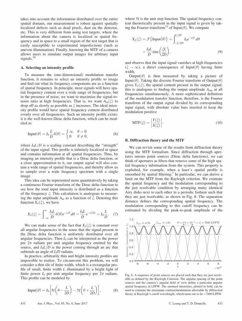
We can revisit some of the results from diffraction theoryusing the MTF formalism. Since diffraction through aper-tures smears point sources (Dirac delta functions), we canthink of apertures as filters that remove some of the high spa-tial frequency information from the system. This property isexploited, for example, when a laser’s spatial profile issmoothed by spatial filtering.1 In particular, we can derive alimit on the MTF from the Rayleigh criterion. We estimatethe spatial frequency and the modulation corresponding tothe just resolvable condition by arranging many identicalAiry disks next to each other in a periodic fashion such thatthey are just resolvable, as shown in Fig. 8. The separationdistance defines the corresponding spatial frequency. Themodulation corresponding to this cutoff frequency can beestimated by dividing the peak-to-peak amplitude of the

Fig. 8. A sequence of point sources are placed such that they are just resolv-

able as defined by the Rayleigh Criterion. The angular spacing of the point

sources and the camera’s angular field of view define a particular angular

spatial frequency in LPPW. The summed intensities, plotted in bold, can be

used to estimate the maximum contrast/modulation allowable by diffraction

theory at Rayleigh’s cutoff wavelength, which turns out to be �7800 LPPW.

433 Am. J. Phys., Vol. 85, No. 6, June 2017 C. Leung and T. D. Donnelly 433

summed intensities by the height of each individual Airydisk.

To estimate the Airy disk size, we write down some typi-cal parameters used in our setup. We fix the aperture size ofthe Canon 40D to 2a¼ 3.5 mm. We assume the light is greenon average, with k¼ 550 nm, and take the object to be at adistance D¼ 70 cm away. The angular separation implied bythe Rayleigh criterion corresponds to a spatial frequency of�7800 LPPW. This can be estimated using the angle sub-tended by the field of view, which is roughly 0.76 rad fromleft to right at a focal length f¼ 28 mm, according to onlinesources including the Canon 40D manual.12 As shown inFig. 8, the contrast at that spatial frequency can be estimatedto be C¼ 0.14. As we will discuss later, the contrast is agood approximation to the modulation in the high-frequencylimit, so we write MTFð7800 LPPWÞ � 0:14.

C. Image acquisition

To measure the modulation transfer function, it is neces-sary to precisely realize the illuminated slit of width L asdescribed in Eq. (8), and then to acquire an image. To pre-cisely realize a slit of width L, a pair of razor blades placedon an adjustable micrometer drive and a black cardboardscreen together obscure all but a thin slit. The razor bladesare aligned by eye to be parallel and oriented such that thesharp edges face each other. Assuming the lens is symmetricabout the lens axis, rotating the slit about the lens axis simplyrotates the image formed on the sensor, providing no newinformation about the optics. However, choosing to orientthe slit along one of the axes of the pixel array maximizesthe Nyquist frequency attained without resorting to sophisti-cated supersampling methods.13 An incandescent lamp isplaced about 2 m behind the razor blades to provide colli-mated, spatially uniform light at the slit. The camera isplaced about half a meter away from the razor blades, andmounted to the breadboard to ensure repeatability. A sche-matic of the entire setup can be seen in Fig. 9, and a closeupof our slit is shown in Fig. 10.

To compare the results from the illuminated slit with theresults from the test targets, camera parameters that signifi-cantly affect the camera’s resolution must be held constantfrom before. The intensity profile of interest, in this case theilluminated slit, should be in the center of the field of view,just as the test targets were. Measurements should be madeat similar distances so the camera’s focus is similar. The

camera’s aperture size should be held constant. We use2a¼ 3.5 mm, which corresponds to f/8.0, to begin with. TheISO and shutter speed are selected as discussed previously.After the camera is aligned, focused, and set to the desiredsettings, an image of the illuminated slit is taken. Asdescribed earlier, a JPG image consisting of 2592� 3888pixels is produced, which can be treated as a 2592� 3888� 3 matrix, where the three layers represent the intensity ineach of the red, green, and blue color bands.

Because modulation measurements are faster to make thancontrast measurements, it is straightforward to quickly mea-sure the MTF at different aperture diameters to characterizethe camera. In addition to measuring the MTF at2a¼ 3.5 mm, we open up the aperture to 2a¼ 8.6 mm corre-sponding to f/3.5. Measuring the MTF at two different aper-ture sizes allows us to observe the opposing effects of lensnonideality and the diffraction limit on the camera’s resolu-tion. As the lens is opened up, the diffraction limit increases.At the same time, spherical aberration is increased becausethe curvature of the lens is no longer negligible as the aper-ture is opened up. In addition, by separating the image intoits constituent red/green/blue channels, we may investigatethe MTF as a function of color band.

D. Data analysis

This section describes how the JPG image of a slit ofwidth L is used to determine the MTF. The input and outputspectra, XLðnÞ and YLðnÞ, can both be fully determined fromthe image.

Given a JPG image, a small rectangular region of interest(ROI) consisting of ðM � NÞ � 3 pixels is selected. Croppingthe image only affects the frequency resolution, leaving theupper limit of the angular frequency (or the Nyquist fre-quency), unchanged. Increasing the number of points in theROI is a tradeoff between increasing the frequency resolutionand increasing the noise, since the signal is localized near thebright slit and pixel readings sufficiently far away from thebright slit contain less information about the camera’sresponse. We experimented with different ROI sizes andfound that M � N ¼ 79� 779 gave good frequency resolu-tion and low noise for a variety of different slit widths, as

Fig. 9. A schematic of the setup used to realize and image a uniformly illumi-

nated slit is shown. An idealization of the camera optics and aperture are shown,

with the camera’s CMOS sensor represented by the dark bar at the far right.

Fig. 10. The slit setup as seen from the source side (i.e., the left side of Fig.

9). The arrows (green online) indicate the razor blades that define the slit.

The blade to the left is mounted on a micrometer drive while the right blade

remains fixed. The black cardboard and the pieces of tape on the razor blade

block stray light from the source.

434 Am. J. Phys., Vol. 85, No. 6, June 2017 C. Leung and T. D. Donnelly 434

shown in Fig. 11. The color bands can either be analyzed sep-arately or aggregated with a weighted average

Igrayscale ¼ crIred þ cgIgreen þ cbIblue; (11)

where ðcr; cg; cbÞ are weights whose exact values depend ondifferent conversions to grayscale taking into account the dif-ferent energies of photons in the different bands, the responseof the human eye, the efficiency of the detectors, etc. Bydefault, MATLAB has a built in function that implements thisconversion, taking ðcr; cg; cbÞ ¼ ð0:2989; 0:5870; 0:1140Þ.14

Regardless of whether color is separated or combined into asingle intensity value according to Eq. (11), we can now dis-cuss how to obtain XLðnÞ and YLðnÞ from a matrix of pixelintensities with M rows and N columns in which the same spa-tial information is encoded in each of the M rows, correspond-ing to Fig. 11.

In the case of the input spectrum, the functional form ofXLðnÞ is known from Eq. (9). Since the zeros of XLðnÞ willshow up as dips in YLðnÞ, we can fit the first zero of the func-tional form of XLðnÞ experimentally, as shown in Fig. 12.The intensity scale of XLðnÞ is set by XLð0Þ ¼ YLð0Þ, sinceMTFð0Þ ¼ 1 by definition. The remainder of this section willfocus on how to obtain smooth estimates of YLðnÞ.

Taking the discrete Fourier transform of each of M rows inthe ROI yields M estimates of the frequency content of theoutput signal YLðnÞ. These estimates, labeled Y1;LðnÞ;…;YM;LðnÞ, are in general complex-valued to reflect the phaseoffset of each frequency component. However, since the MTFdoes not encode phase information and is a real, positivequantity, we ignore the phase factor and average the magni-tudes over the M estimates to provide a smoother estimate ofthe real, positive output spectrum YLðnÞ, or

YL nð Þ ¼ 1

M

XM rows

i¼1

jYi;L nð Þj: (12)

The same procedure repeated with the lamp turned offprovides an estimate of the (real and positive) noise floor dueto electronic cross-talk, stray light, etc. To a very goodapproximation, this noise floor NðnÞ is independent of theslit width, so we do not denote it with a subscript L. Thethree spectra XLðnÞ; YLðnÞ;NðnÞ are plotted in Fig. 12. Theresulting MTF estimate MTFLðnÞ ¼ YLðnÞ=XLðnÞ is plottedin Fig. 13.

The obvious problem with Fig. 13 is that it features a spu-rious peak which is clearly unphysical in nature. This behav-ior is a result of our measurements having YLðnÞ > 0everywhere due to the finite noise floor, whereas XðnÞ ¼I0L=DjsincðnL=2DÞj has zeros at n ¼ 2npD=L; n ¼ 1; 2;…,one of which is seen in Fig. 12. One solution is to use valuesof L that are so narrow that the finite pixels cannot distin-guish the slit from an infinitely thin impulse. This approachruns into difficulties because as the slit gets narrower, thereis not enough light incident on the detector to maintain agood signal-to-noise ratio, as discussed in Eq. (9). On theother hand, as the slit gets wider, the spurious peaks in theMTF estimates are shifted to lower and lower frequencies.

A robust solution is to take a weighted average of multipleMTF estimates over several slit widths chosen to be not toonarrow and not too wide. In our experiment, six such widthsranging from 0.21 to 1.06 mm are used and are listed inTable I. The “weights” in the weighted average are taken tobe the relative signal-to-noise ratio at each frequency. For aparticular slit width L, we can define the signal-to-noise ratioas a function SNRLðnÞ of the angular frequency n as

SNRL nð Þ ¼ XL nð ÞN nð Þ ; (13)

Fig. 12. Assuming an input spectrum of the form XðnÞ ¼ ðI0L=DÞjsincðnL=2DÞj, we fit the first zero of the input spectrum by estimating the

minimum of the experimental data.

Fig. 13. Plotting YLðnÞ=XLðnÞ from the data shown in Fig. 12 reveals a spuri-

ous peak in the MTF estimate, a result of the fact that the analytically

defined input spectrum XLðnÞ vanishes for certain values of n while the

experimentally measured output spectrum YLðnÞ contains noise.

Fig. 11. The region of interest shown is cropped from a larger JPG image of

the slit. The dimensions of the region of interest are chosen to strike a balance

between frequency resolution and increased noise. Discrete Fourier transforms

are taken along the horizontal axis to obtain a number of different output spec-

trum estimates. This particular image was taken at a slit width of 1.06 mm.

Table I. Angular spatial frequencies n for different slit widths. The slit

widths were measured to a precision of 1 lm with a micrometer drive on the

translation stage. The first few frequency values were measured experimen-

tally, and since the first zero of XLðnÞ scales as 1=L, the higher values are

extrapolated to some extent (the extrapolated values are indicated with an

asterisk).

Slit width [mm] n of first zero [LPPW]

1.060 1013

0.860 1273

0.660 1812

0.460 2670

0.260 4480*

0.210 5546*

435 Am. J. Phys., Vol. 85, No. 6, June 2017 C. Leung and T. D. Donnelly 435

with the relative signal-to-noise ratio defined as

RSNRLinð Þ ¼ SNRLi

nð ÞXall L

SNRL nð Þ: (14)

As we would like the weight RSNRLðnÞ on a particular mea-surement YLðnÞ vanishes at the frequencies where the inputsignal XLðnÞ vanishes, the sum of the RSNR weights is 1.Hence, the spurious peaks, such as the one seen in Fig. 13,do not end up affecting the MTF estimate significantly.

We form a weighted average of MTF estimates over thevalues of L tabulated in Table I, which turns out to be equiv-alent to measuring the sum of the output signals divided bythe sum of the input signals. The individual MTF estimatesat six different slit widths and their weighted average are

MTF nð Þ ¼Xall L

RSNRL nð ÞMTFL nð Þ ¼

Xall L

YL nð ÞXall L

XL nð Þ; (15)

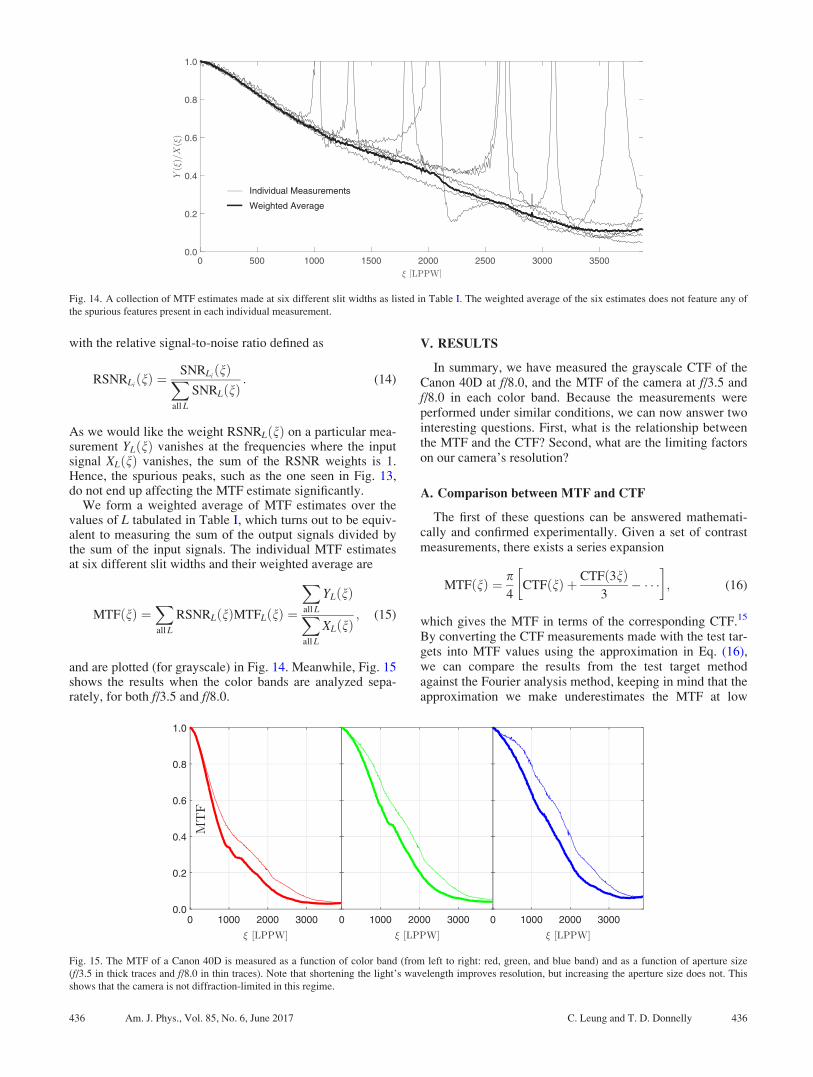
and are plotted (for grayscale) in Fig. 14. Meanwhile, Fig. 15shows the results when the color bands are analyzed sepa-rately, for both f/3.5 and f/8.0.

V. RESULTS

In summary, we have measured the grayscale CTF of theCanon 40D at f/8.0, and the MTF of the camera at f/3.5 andf/8.0 in each color band. Because the measurements wereperformed under similar conditions, we can now answer twointeresting questions. First, what is the relationship betweenthe MTF and the CTF? Second, what are the limiting factorson our camera’s resolution?

A. Comparison between MTF and CTF

The first of these questions can be answered mathemati-cally and confirmed experimentally. Given a set of contrastmeasurements, there exists a series expansion

MTF nð Þ ¼ p4

CTF nð Þ þ CTF 3nð Þ3

� � �

; (16)

which gives the MTF in terms of the corresponding CTF.15

By converting the CTF measurements made with the test tar-gets into MTF values using the approximation in Eq. (16),we can compare the results from the test target methodagainst the Fourier analysis method, keeping in mind that theapproximation we make underestimates the MTF at low

Fig. 14. A collection of MTF estimates made at six different slit widths as listed in Table I. The weighted average of the six estimates does not feature any of

the spurious features present in each individual measurement.

Fig. 15. The MTF of a Canon 40D is measured as a function of color band (from left to right: red, green, and blue band) and as a function of aperture size

(f/3.5 in thick traces and f/8.0 in thin traces). Note that shortening the light’s wavelength improves resolution, but increasing the aperture size does not. This

shows that the camera is not diffraction-limited in this regime.

436 Am. J. Phys., Vol. 85, No. 6, June 2017 C. Leung and T. D. Donnelly 436

angular frequencies. Interestingly, since both the MTF andCTF tend toward zero in the high-frequency limit, thehigher-order terms in Eq. (16) vanish faster than the CTFðnÞterm. That is, the CTF converges to the MTF up to a constantas n gets large, so that

MTF nð Þ � p4

CTF nð Þ: (17)

Experimentally, this agreement is seen at high frequencies asexpected (see Fig. 16).

The tradeoffs of using contrast versus modulation to quan-tify a system’s optical quality are clear from Fig. 16. On theone hand, measuring the contrast is much more intuitive andstraightforward than measuring the modulation and does notrequire the same amount of averaging to obtain meaningfulresults. On the other hand, measuring the contrast at manypoints is much more tedious. Naturally, choosing betweenone quantification method or another depends on what infor-mation is relevant. If the falloff rate of the spatial resolutionas a function of frequency is not of interest, it is more practi-cal to specify a contrast threshold and measure the frequencycorresponding to that threshold. In many situations, however,the MTF is more valuable to have. For example, astronomersroutinely measure the MTF of telescopes and imaging cam-eras in order to estimate the size of astronomical objectsfrom telescope images.16

B. Limits on resolution

We know that for even the most ideal camera, diffractionis the ultimate downfall of resolution. But how close to idealis our Canon 40D? In this section, we discuss possible limit-ing factors on the resolution and conclude that sphericalaberration, rather than pixelation, chromatic effects, or dif-fraction, is the most likely culprit.

Recall that we derived theoretically that MTFð7800 LPPWÞ� 0:14 corresponds to an angular separation implied by theRayleigh criterion. Since this spatial frequency corresponds toan angular size smaller than a pixel (whose angular size corre-sponds to 3888 LPPW), we determine that our consumer-grade imaging system is not operating near the Rayleigh limit.

Pixelation is another concern. The fact that pixelationcauses the image of a point source to instead look like a

square the size of a pixel allows us to infer the functionalform of the MTF contribution due to pixelation. If pixelationwere the limiting factor on the resolution, the resolutionshould fall off like sincðn=3888 LPPWÞ. However, as seen inFig. 15, the resolution falls off far more rapidly and has astrong dependence on the aperture size, leading us to rule outthis hypothesis.

From the same set of data, Fig. 15, we can rule out chro-matic, or color-dependent, aberration as the dominant contri-bution to our resolution. The data show that the qualitativewavelength dependence is as predicted by scalar diffractiontheory for both large and small aperture sizes—the resolutionimproves as the wavelength is decreased. We conclude thatchromatic aberration is not the limiting factor on the Canon40D’s resolution.

Finally, we consider spherical abberation, an effect thatoccurs in imaging systems where the thin-lens approximationbreaks down. This effect becomes more pronounced as theaperture is opened wider.1 Our data show that when the aper-ture size is increased to 2a¼ 8.6 mm, the resolutiondecreases. We conclude that spherical aberration is likely thelimiting factor on the resolution.

It is plausible that the camera’s designers have carefullyoptimized the resolution limits of all of the components inthe body of the camera—the pixel array, electronics, etc.—tominimize the cost of the camera. At the same time, photogra-phy connoiseurs have the option to improve the system’sperformance by replacing the stock lens with a specializedlens to suit their imaging needs. In this way, the Canon 40Dcan cater to a wide range of consumers at minimal base cost.This sensible design choice is a direct reflection of the richscience and engineering that goes into making a camera.

VI. CONCLUSION

We have demonstrated a number of ways to quantify theresolution of a camera with a relatively simple experimentalsetup, including using the Rayleigh Criterion, the contrasttransfer function (CTF), and finally the modulation transferfunction (MTF). Our measurements suggest that the resolu-tion of a typical DSLR such as the Canon 40D is limited byits optical subsystem, namely, spherical aberration. Thisexperiment provides a concrete introduction to cornerstoneconcepts of modern optics, including Fourier analysis, dif-fraction theory, and analysis techniques to resolve informa-tion in spatial data. The emphasis placed on overcomingpractical problems dealt with in the MTF measurement (i.e.,making measurements that are robust against noise) makesthe experiment described well-suited for the undergraduatelaboratory and for students going on in the optics/photonicsindustry.3

ACKNOWLEDGMENTS

The authors thank Professors Richard Haskell, Peter Saeta,and Patricia Sparks for helpful discussions. This investigationwould not have been possible without their support.

APPENDIX A: SUGGESTED BILL OF MATERIALS

Included in Table II is a suggested bill of materials to usein building this experiment. We did not have an adjustablemechanical slit and built our own without much difficultyout of translation stages, right angle brackets, and two

Fig. 16. Contrast measurements made from the test targets at f/8.0 shown in

Fig. 4 are converted to modulation using Eq. (16). These values are com-

pared to our MTF measurements made under similar conditions with the

illuminated slit. As expected, the test-target measurement underestimates

the modulation at low frequencies, and the two measurements converge as nincreases.

437 Am. J. Phys., Vol. 85, No. 6, June 2017 C. Leung and T. D. Donnelly 437

commercially available razor blades. Though our setup wasmounted to a breadboard, mechanical vibrations were notfound to be the limiting factor in our ability to make robustmeasurements.

1M. Born and E. Wolf, Principles of Optics: Electromagnetic Theory ofPropagation, Interference and Diffraction of Light (Cambridge U. P.,

Liberty Plaza Floor 20. New York NY 10006, 2000), pp. 370–433.2G. D. Boreman, Modulation Transfer Function in Optical and Electro-Optical Systems (SPIE Press, Bellingham, 2000), pp. 1–61.

3D. C. O’Shea, “Transition to reality: Preparing the student at Georgia Tech

through an undergraduate sequence of optics laboratories,” Educ. Opt.

1603, 317–324 (1992).

4A. P. Tzannes and J. M. Monney, “Measurement of the modulation trans-

fer function of infrared cameras,” Opt. Eng. 34, 1808–1817 (1995).5H. Fujita, D.-Y. Tsai, T. Itoh, J. Morishita, K. Ueda, and A. Ohtsuka, “A

simple method for determining the modulation transfer function in digital

radiography,” IEEE Trans. Med. Imaging 11, 34–39 (1992).6D. C. O’Shea, “A modulation transfer function analyzer based on a micro-

computer and dynamic ram chip camera,” Am. J. Phys. 54, 821–854 (1986).7G. B. Airy, “On the diffraction of an object-glass with circular aperture,”

Cambridge Philos. Soc. Trans. 5, 283 (1835).8J. Strutt, “On the theory of optical images, with special reference to the

microscope,” Philos. Mag. 42, 167–195 (1896).9In this study, we used http://digicamcontrol.com/digiCamControl, which is open

source, available at no charge, and is compatible with a wide range of cameras.10Of course, to handle two dimensional images, one needs to generalize the

definition of the MTF to two dimensions.11Readers familiar with scalar diffraction theory will notice the similarity

between the functional form of ½XLðnÞ2 and the Fraunhofer diffraction pat-

tern projected onto a screen by a coherently illuminated rectangular slit.1

The connection between Fourier transforms and diffraction is profound

but outside the scope of this paper.12EOS 40D Instruction Manual (Canon Inc., Lake Success, NY 11042,

USA, 2007), pp. 181–188.13P. Burns, “Slanted-edge MTF for digital camera and scanner analysis,” in

Proceedings of the IS&T’s PICS Conference (2000), pp. 135–138.14L. Benedetti, M. Corsini, P. Cignoni, M. Callieri, and R. Scopigno, “Color

to gray conversions in the context of stereo matching algorithms,” Mach.

Vision Appl. 23, 327–348 (2012).15J. W. Coltman, “The specification of imaging properties by response to a

sine wave input,” J. Opt. Soc. Am. 44, 468–471 (1954).16R. Lupton, J. E. Gunn, Z. Ivezic, G. R. Knapp, S. Kent, and N. Yasuda,

“The SDSS imaging pipelines,” ASP Conf. Ser. 10, 269–278 (2001).17U.S. Department of the Air Force, Military Standard Photograph Lenses

(U.S. Government Publishing Office, Washington DC., 1959), p. 21.

Table II. A suggested bill of materials to be used in building this experi-

ment. Standard hardware like an optical breadboard and bolts are not

included.

Item Cost

Digital camera, e.g., Canon EOS 40D (used) $300

Lens, e.g., Canon EF 28–135 mm f/3.5–5.6 IS USM $300

Camera remote trigger $10

Mini-USB transfer cable $5

Thorlabs adjustable mechanical slit VA100 $248

1951 Air force resolution test targets $10

Table lamp $10

Black cardboard for stray light blockage $5

Total $890

438 Am. J. Phys., Vol. 85, No. 6, June 2017 C. Leung and T. D. Donnelly 438