Labor Supply, Wealth Dynamics, and Marriage Decisions
53
Labor Supply, Wealth Dynamics, and Marriage Decisions * Maurizio Mazzocco Claudia Ruiz Shintaro Yamaguchi UCLA World Bank McMaster University First Draft July 2005, Current Draft December 2013 Preliminary Abstract Using the Panel Study of Income Dynamics (PSID), we provide evidence that labor supply, household production, savings, and marital decisions are linked. We then develop and estimate a model that has the ability to generate the patterns observed in the data. Using the estimated model we first show that it is important to consider the link between labor supply, household production, wealth, and marriage choices to understand household behavior and its response to policy changes. We then use the model to evaluate the effect of the Earned Income Tax Credit (EITC) and other subsidy programs on individual decisions and welfare. ∗ We are very grateful to Moshe Buchinsky, Pierre-Andr´ e Chiappori, Lucas Davis, James Heckman, Joseph Hotz, John Kennan, James Walker, Victor Rios-Rull, Duncan Thomas, and participants at SITE, the Econometric Society World Congress, the Minnesota Applied Micro Workshop, the Queen’s University Quantitative Economics Workshop, UCLA, and the Conference on Households, Gender and Fertility at UC Santa Barbara for their helpful comments. Mazzocco thanks the National Science Foundation for Grant SES-0519276, and the Academic Technology Services at UCLA and the San Diego Supercomputer Center for the use of their computer clusters. 1
Transcript of Labor Supply, Wealth Dynamics, and Marriage Decisions

Labor Supply, Wealth Dynamics, and Marriage Decisions∗
Maurizio Mazzocco Claudia Ruiz Shintaro Yamaguchi
UCLA World Bank McMaster University
First Draft July 2005, Current Draft December 2013
Preliminary
Abstract
Using the Panel Study of Income Dynamics (PSID), we provide evidence that labor supply,
household production, savings, and marital decisions are linked. We then develop and estimate
a model that has the ability to generate the patterns observed in the data. Using the estimated
model we first show that it is important to consider the link between labor supply, household
production, wealth, and marriage choices to understand household behavior and its response to
policy changes. We then use the model to evaluate the effect of the Earned Income Tax Credit
(EITC) and other subsidy programs on individual decisions and welfare.
∗We are very grateful to Moshe Buchinsky, Pierre-Andre Chiappori, Lucas Davis, James Heckman, Joseph Hotz,
John Kennan, James Walker, Victor Rios-Rull, Duncan Thomas, and participants at SITE, the Econometric Society
World Congress, the Minnesota Applied Micro Workshop, the Queen’s University Quantitative Economics Workshop,
UCLA, and the Conference on Households, Gender and Fertility at UC Santa Barbara for their helpful comments.
Mazzocco thanks the National Science Foundation for Grant SES-0519276, and the Academic Technology Services
at UCLA and the San Diego Supercomputer Center for the use of their computer clusters.
1

1 Introduction
Many of the policies discussed by policy makers and economists affect the decisions and welfare of
individuals and of the households in which they live. The most common examples are changes to
the tax code or changes to programs for low-income families such as the Earned Income Tax Credit
(EITC), unemployment benefits, or food stamp programs. To evaluate whether these changes are
socially beneficial, it is important that economists and policy makers understand their effect on
individual and household decisions.
The first contribution of this paper is to show empirically that different types of household
decisions, namely labor supply, household production, savings, and marital decisions, are intercon-
nected. As a consequence, to evaluate the effect of a particular policy on individual decisions and
welfare, economists and policy makers should not consider its impact on one type of decision at a
time, but rather on all of them simultaneously. Specifically, using the Panel Study of Income Dy-
namics (PSID), we find that households display large differences in labor supply, savings, and time
devoted to household production by marital status. Married men work on average about 200 hours
more than single men, who work 200 hours more than single women, whose labor hours exceed the
labor hours of married women by about 200 hours. The same ranking applies to labor force par-
ticipation. Married men have the highest participation rate, followed by single men, single women,
and married women. The ranking for household production is reversed. Married women spend
the highest number of hours in household production at 1287 annual hours. They are followed by
single women with 604 annual hours, single men with 372 hours, and married men with 366 hours.
Households display large differences by marital status also with respect to savings decisions. In
the PSID, married couples on average have more than four times the wealth of individuals who
are single and more than twice the wealth of married couples that will experience a divorce in the
following year.
In the paper, we provide evidence that the differences between married and single individuals
in labor supply and household production observed in the PSID data do not arise suddenly at the
time of marriage, but rather emerge gradually over time. To document this pattern, we study the
evolution of these variables for women and men who experience a marriage or a divorce. We show
that, before women choose to marry, they supply on average the same amount of labor hours as the
average single woman. Starting from two years before marriage, however, they begin to gradually
reduce their labor hours. At the time of marriage, their labor supply is about 200 hours lower
than the average single woman and about 300 hours higher than the average married woman. The
labor supply of women who experience this transition into marriage continue to decline until after
4-5 years of marriage it reaches the level of the average married woman. The labor supply of men
2

who enter marriage displays a similar transition but with a positive trend. Prior to marriage, they
supply the same amount of labor hours as the average single man. Beginning from two years before
marriage, this group of men starts to increase their labor supply. At the time of marriage, their
labor supply is about 150 hours larger than the average labor supply of single men and about 100
hours less than the average married man. After they enter marriage, their labor supply continues
to increase until the fourth year of marriage when it reaches the level of the average married man.
As an additional result, we provide evidence that when women transition into fewer labor hours,
they adjust accordingly the time they spend in household production. Specifically, the year before
marriage, women start to increase the number of hours they devote to household production from
the level supplied by the average unmarried woman. The rise in hours then continues until after
five years of marriage it converges to the amount supplied by the average married women.
The transition of married couples into divorce is also characterized by significant changes in labor
supply and time spent in household production. Well before a divorce occurs, married households
start reducing the degree of intra-household specialization. The changes affect mostly women.
Their labor supply begins to increase three years before a divorce is observed and keeps increasing
until the first year after divorce when it reaches the level that characterizes the average single
woman. Men do not change their labor supply before a divorce, but adjust the number of labor
hours after the event. Three years after a divorces, the average men supplies the same amount of
labor hours as the average single man.
The evidence provided in the first part of the paper indicates that to understand the effect of
policy interventions on household decisions and individual welfare, one has to take into account the
relationship between different aspects of household behavior. Most studies that analyze household
decisions ignore this relationship and focus on a subset of household choices. The main goal of the
second part of the paper is to develop a model that considers simultaneously labor supply, household
production, savings, and marital decisions. A model that can therefore be used to evaluate the
benefits and costs of the many policies that have an impact on individual welfare.
In the model that we propose, individuals who are single meet potential spouses and decide
whether to marry. Married couples make decisions cooperatively, in the sense that they are efficient.
But, given that non-consensual divorces are frequent in the U.S. data, we do not allow them to
commit to future allocations of resources. A couple divorces when the marriage no longer generates
a positive surplus and therefore both spouses are better off as single. The inability of spouses to
commit implies that the relative decision power of each household member varies with changes
in their outside options. This has two main implications. First, saving decisions and decisions
related to labor hours and time spent in household production change over time not only because
of variation in interest rates and wages, but also because of changes in the relative intra-household
3
decision power. Second, savings and time allocation decisions affect the individual outside options
and therefore the individual decision power.
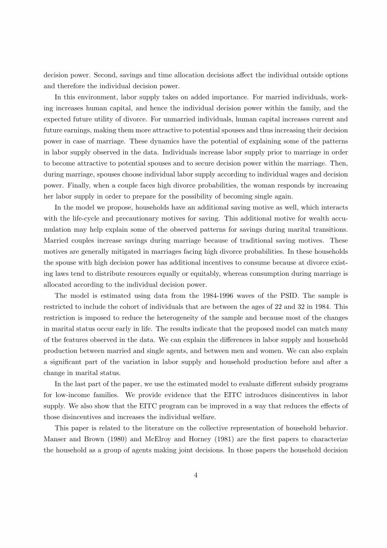
In this environment, labor supply takes on added importance. For married individuals, work-
ing increases human capital, and hence the individual decision power within the family, and the
expected future utility of divorce. For unmarried individuals, human capital increases current and
future earnings, making them more attractive to potential spouses and thus increasing their decision
power in case of marriage. These dynamics have the potential of explaining some of the patterns
in labor supply observed in the data. Individuals increase labor supply prior to marriage in order
to become attractive to potential spouses and to secure decision power within the marriage. Then,
during marriage, spouses choose individual labor supply according to individual wages and decision
power. Finally, when a couple faces high divorce probabilities, the woman responds by increasing
her labor supply in order to prepare for the possibility of becoming single again.
In the model we propose, households have an additional saving motive as well, which interacts
with the life-cycle and precautionary motives for saving. This additional motive for wealth accu-
mulation may help explain some of the observed patterns for savings during marital transitions.
Married couples increase savings during marriage because of traditional saving motives. These
motives are generally mitigated in marriages facing high divorce probabilities. In these households
the spouse with high decision power has additional incentives to consume because at divorce exist-
ing laws tend to distribute resources equally or equitably, whereas consumption during marriage is
allocated according to the individual decision power.
The model is estimated using data from the 1984-1996 waves of the PSID. The sample is
restricted to include the cohort of individuals that are between the ages of 22 and 32 in 1984. This
restriction is imposed to reduce the heterogeneity of the sample and because most of the changes
in marital status occur early in life. The results indicate that the proposed model can match many
of the features observed in the data. We can explain the differences in labor supply and household
production between married and single agents, and between men and women. We can also explain
a significant part of the variation in labor supply and household production before and after a
change in marital status.
In the last part of the paper, we use the estimated model to evaluate different subsidy programs
for low-income families. We provide evidence that the EITC introduces disincentives in labor
supply. We also show that the EITC program can be improved in a way that reduces the effects of
those disincentives and increases the individual welfare.
This paper is related to the literature on the collective representation of household behavior.
Manser and Brown (1980) and McElroy and Horney (1981) are the first papers to characterize
the household as a group of agents making joint decisions. In those papers the household decision
4
process is modeled by employing a Nash bargaining solution. Chiappori (1988) and Chiappori
(1992) extend their model to allow for any type of efficient decision process. The theoretical model
used in the present paper is a generalization of the static collective model introduced by Chiappori to
an intertemporal framework without commitment. The static collective model has been extensively
tested and estimated. Thomas (1990) is one of the first papers to test the static unitary model
against the static collective model. Browning et al. (1994) perform a similar test and estimate the
intra-household allocation of resources. Chiappori, Fortin, and Lacroix (2002) analyze theoretically
and empirically the impact of the marriage market and divorce legislations on household labor
supply using a static collective model. Blundell et al. (2007) develop and estimate a static collective
labor supply framework which allows for censoring and nonparticipation in employment. Donni
(2004) shows that different aspects of a static collective model can be identified and estimated.
This paper also contributes to a growing literature which attempts to model and estimate the
intertemporal aspects of household decisions using a collective formulation. Lundberg, Startz,
and Stillman (2003) use a collective model with no commitment to explain the consumption-
retirement puzzle. Guner and Knowles (2003) simulate a model in which marital formation affects
the distribution of wealth in the population. van der Klaauw and Wolpin (2008) formulate and
estimate a model of retirement and saving decisions of elderly couples who make efficient decisions.
Duflo and Udry (2004) study the resource allocation and insurance within households using data
from Cote D’Ivoire. Rios-Rull, Short, and Regalia (2010) develop a model in which men and women
make marital status, fertility, and investment in children decisions conditional on the available wage
distribution. The model is then used to explain the large increase in the share of single women
and single mothers between the mid seventies and the early nineties. Mazzocco (2004) analyzes the
effect of risk sharing on household decisions employing a full-commitment model. Mazzocco (2007)
tests three models: the intertemporal unitary model, the full-commitment intertemporal collective
model, and the no-commitment collective model. The data reject the first two models in favor of
the no-commitment model. Tartari (2007) employs a dynamic model of the household to evaluate
the effect of divorce on the cognitive ability of children. Casanova (2010) is one of the first papers to
study retirement decisions as the joint decision of husband and wife using a collective model of the
household with commitment. Gemici (2011) analyzes migration family choices when both spouses
are involved in the decision process. Gemici and Laufer (2011) consider the effect of cohabitation on
future household decisions and individual welfare using a no-commitment model of the household
similar to the one considered here. Voena (2011) evaluates the effect of changes in divorce laws
in the late sixties and early seventies on labor supply of single and married individuals using a
framework similar to the one employed in this paper. Fernandez and Wong (2011) attempt to
explain the larger increase in labor force participation of women in the second half of the twentieth
5

century using a dynamic model of household decisions.
Many papers have analyzed labor supply decisions by gender and marital status. For instance,
Heckman and Macurdy (1980) estimate a life cycle model of labor supply decisions of married fe-
males. Jones, Manuelli, and McGrattan (2003) and Olivetti (2006) study the large increase in labor
supply of married women in the United States in the second half of the twentieth century. Andres,
Fuster, and Restuccia (2005) document gender differences in wages, employment and hours of work
during the life cycle. They use a model with fertility decision and human capital accumulation
to rationalize the empirical patterns. The present paper is, however, one of the first attempts to
estimate a model of labor supply decisions that considers the transitions in and out of marriage.
The paper proceeds as follows. The next section documents the patterns observed in the PSID.
Sections 3 and 4 describe the no-commitment intertemporal collective model. Sections 5 and 6
explain how the model is estimated and present the results. In section 7, we describe a set of policy
evaluations. Section 8 concludes.
2 Empirical Evidence
This section presents empirical evidence which indicates that labor supply, household production,
savings, and marital decisions are related. The discussion is based on data from the Panel Study
of Income Dynamics (PSID). The PSID is well suited to analyze the relationship between labor
supply, saving, and marital decisions for two reasons. First, the PSID has gathered individual-level
data on labor supply, time spent on household production, and marital status annually each spring
since 1968 and data on household wealth every four years starting in 1984. Second, since the PSID
is a true panel that follows the same households and their split-offs over time, the dataset can be
used to examine the dynamics of household decisions.
Table 1 summarizes some of the household decisions made by unmarried females, married
females, unmarried males, and married males. The sample covers the period 1968-1996 and is
restricted to include individuals between the ages of 20 and 40. The latino and immigrant samples
are excluded from the analysis. These restrictions are used to reduce the heterogeneity in the
sample and because most of the changes in marital status occur at young ages.
Table 1 displays some features of household behavior that are worth discussing. First, there
is a clear pattern by gender and marital status in labor supply behavior: married men work more
than unmarried men, who work more than umarried women, who choose to supply more hours
than married women. Specifically, conditional on working, unmarried females supply on average
about 200 more hours a year than married females. The annual labor supply of unmarried men is
lower than the labor supply of married men by slightly more than 200 hours. Both unmarried and
6

married women supply fewer hours on the labor market than men. Second, labor force participation
of single men is only 2% lower than labor force participation of married men which is equal to 98%.
Unmarried women are five percentage points less likely to work than unmarried men. As expected,
married women are less likely to work in the labor market with a participation rate of 66%. Hours
spent on household production display a pattern that is consistent with the data on labor supply:
the individuals that supply longer labor hours devote less time to household production. Married
women are the top of the ranking with 1287 annual hours, followed by single women with 604.
Next in the ranking we find single men with 372 hours and, in the last position, married men who
devote about the same amount of hours to household production as single men at 366.
The numbers in Table 1 give a static picture of the relationship between labor supply, household
production, and marriage decisions. To provide a more dynamic description of the link among these
decisions, we now describe the evolution of labor supply and household production decisions around
the time a couple chooses to marry. Figures 1-6 describe labor supply decisions as individuals enter
marriage relative to two baseline comparison groups: married individuals and single individuals.
An index is used where 0 denotes the first year of a transition between marital states. The index
-t indicates the t-th year prior to the transition and t indicates the t-th year after the transition.
These marriages occur during different years in the sample for different individuals. In some cases
particular observations will not be available for particular individuals. For example, an observation
for three years prior to marriage will not be available for an individual who gets married in the
second year of the sample. For this reason the number of observations will vary at different points
in the index. To take this into account, we weight the baseline comparison groups to reflect the
calendar year composition of the transition groups.
Figure 1 describes women’s labor supply before and during marriage. During the transition,
average annual labor supply falls from the average number of hours supplied by single women,
around 1600, to the average amount of labor hours supplied by married women, around 1100
hours. This large decline begins two years prior to marriage and continues many years into the
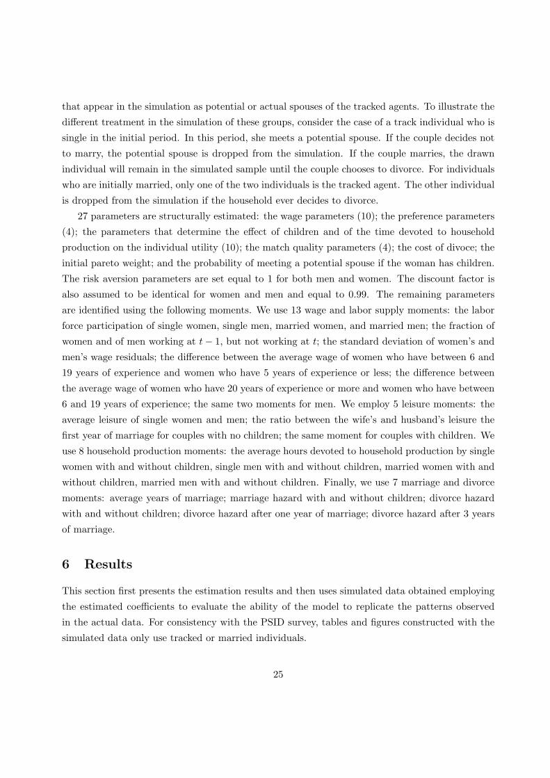
marriage. Figures 3 and 5 describe similar patterns for labor supply conditional on working and
labor force participation. Figure 2 reports the evolution of the same variables for men. The labor
supply behavior of men shows a pattern similar to the one displayed by women, but with a trend
that goes in the opposite direction. When women start decreasing their labor supply about two
years before marriage, men begin to increase their labor hours. They continue to increase the
amount of labor hours until their fourth year of marriage when they reach the level of the average
married man. During the transition men increase their labor supply by about 300 hours. Figures
4 and 6 display labor supply conditional on working and labor force participation for the same
sample of men.
7

In the next two figures, we describe the evolution of the time spent on household production by
women and men. Figure 7 shows that the large decline in labor supply of women around the year
of marriage is accompanied by a similar increase in time devoted to household production. This
rise starts the year before the woman marries and continues for the first five years of marriage.
After the transition, women supply on average 600 more hours to household production than the
average single woman. In Figure 8, we report the evolution of the same variable for men. Given
that there is no difference in household production between single and married men, there is also
no transition for this variable for men that enter a marriage.
One possible explanation for the changes in labor supply behavior around the time of marriage
is that marriage proxies for the time of the first birth. To evaluate whether this is the case, in
Figures 9 and 10 we show the evolution of labor supply of women and men before and after the
first birth. The birth of the first child explains a significant fraction of the decline in labor supply
of women before and during marriage. Their average labor supply decreases from about 1600 hours
two years before the first birth to about 900 hours in the year of the first birth. The decline is
explained by a drop in the number of hours conditional on working as well as by a reduction in
labor force participation. Men display a different pattern. Their labor supply increases steadily
starting three years before the birth of their first child and ending two years after the first child
was born. The increase in labor supply is almost entirely explained by the increase in hours worked
conditional on participation. Since the transition in the labor supply of men starts well before the
birth of the first child and continues afterward, our results suggest that their transition in labor
supply is not generated exclusively by a birth.
To determine whether for women the entire transition is explained by the birth of a child, Figure
11 depicts the labor supply decisions of women without children before and during marriage. This
group of women displays a decrease in labor supply before and during marriage even if they do
not have children. This last result implies that the variation in labor supply of women observed
around marriage is not exclusively explained by children. We have also looked at the changes in
labor supply decisions of men without children. Figure 12 indicates that for this selected sample
there is no transition in labor supply.
To investigate the role of labor market experience and education on the decisions of women
around the time of marriage, in figure 13 and 14 we graph the residuals obtained by regressing
labor supply of women without children and men on education and on a polynomial of second
order in experience. The objective is to understand whether accumulated human capital explains
the variation in labor supply that is not explained by children. Accumulated human capital explains
part of the observed changes in labor supply. However, for both women without children and men
we still observe the labor supply transition discussed above.
8

The next set of figures studies the effect of divorce on labor supply and household production
decisions. Figure 15 describes labor supply of women before and after divorce. Our results indicate
that the intra-household specialization that is generated during marriage disappears in the years
that precede a divorce. Specifically, five years before a divorce, women work on average the same
amount of hours as the average married woman. Starting from three years before a divorce, however,
women start to increase their labor supply. At the time of divorce, women supply about 400 labor
hours more than the average married woman and about 150 hours less than the average single
woman. Then one year after divorce, women going through this transition work as much as the
average single woman. These results are consistent with the results presented in Johnson and
Skinner (1986). Figure 16 describes the evolution of labor supply for men that experience a divorce.
During marriage they work the same amount of hours as the average married man. It is only after
divorce that they reduce their labor supply by about 200 hours.
In the next set of figures, we describe the evolution of household production before and after
divorce. Figures 17 and 18 describe the amount of hours spent by women and men on household
production before and after divorce. They show that the labor supply changes experienced by
women are matched by changes in the amount of time they devote to household production. When
women increase their market labor before a divorce, they reduce the time spent on household
production by about the same amount. As a consequence their leisure remains roughly unchanged
during this transition. In the figure for men there is nothing remarkable, which is not surprising
given that there is no difference between the time spent on household production by married and
single men.
We conclude this section with a discussion of the differences in wealth holding by marital
status. Real estate values and the value of cars are excluded from our definition of wealth. Table
2 indicates that wealth levels vary with marital decisions. Married couples have on average more
than four times the wealth of umarried individuals. This difference grows over time since at the
time of marriage couples have slightly less than twice the wealth of unmarried individuals. It is
also noteworthy that couples that will experience a divorce in one year have on average less than
half the wealth level of married couples.
This section provides evidence that labor supply, household production, savings, and marriage
decisions are related. Traditional studies of labor supply have focused on married individuals only
or single individuals only, therefore ignoring the relationship among these variables. The rest of the
paper is devoted to developing and estimating a model that can generate the link between labor
supply, household production, wealth, and marital choices observed in the data.
9

3 The Model
In this section we develop a model that has the potential of generating the empirical patterns
observed in the data. To explain those patterns, a model must be able to generate a type of intra-
household specialization which has the following two features. First, the specialization starts before
marriage and increases after the household has been formed. Second, the specialization decreases
before a divorce. The empirical evidence suggests that the change over time in specialization is
partially explained by the following two variables: the birth of children and by the accumulation of
human capital. The data also indicate that there is a residual part of the evolution of specialization
that these two variables cannot explain. The model should therefore include children, the evolution
of human capital, and an additional source of specialization that can explain its residual component.
Specifically, we will consider a model with the following features. There are two types of
individuals: women and men. Each one of them lives for T periods in an environment characterized
by uncertainty, which is captures by the states of nature ω ∈ Ω. Each individual enters the period
as married or single. If she is single, she draws from the population a potential spouse. They must
then decide whether to get married. If she is married, her and her spouse must decide whether to
stay married. In case of divorce, a cost D must be paid.
One can use different approaches to characterize the decision process of married individuals.
The degree of intra-household specialization observed in the data suggests, however, that there
is some level of cooperation in the majority of married households. We will therefore use a co-
operative framework to represent their decision process. In a static framework, the cooperative
model generally used is the collective model, whose main feature is the assumption that household
decisions are efficient. When the collective model is extended to an intertemporal environment, a
commitment issue arises. One can consider a model in which the married individuals can commit
to future plans. In this case the individuals choose a contingent plan at the time of marriage and
stick to it even if ex-post it would be optimal to renegotiate the initial agreement or divorce. As an
alternative, one can consider a model with no commitment. In this case, the married individuals
renegotiate the initial plan or divorce if it is optimal. It is equivalent to requiring that the con-
tingent plan satisfies a set of participation constraints in each period and state of nature, i.e. the
expected welfare of each individual if she stays married is greater than the expected welfare provide
by the best outside option.1 Mazzocco (2007) tests the full-commitment and the no-commitment
intertemporal collective models. Using US data the full-commitment model is rejected, whereas
the no-commitment model cannot be rejected. For this reason, we will characterize the decision
1The model used here builds on the approach developed in the no-commitment literature. See for example Marcet
and Marimon (1992), Marcet and Marimon (1998), Kocherlakota (1996), Attanasio and Rios-Rull (2000) and Ligon,
Thomas, and Worrall (2002), and Mazzocco (2007).
10
process of married households using an intertemporal collective model with no commitment. Since
the cost of divorce in the US is generally low, we use divorce as the best outside option for married
individuals. In the no-commitment model, the difference between the value of being married and
the value of divorce for two married individuals characterizes the marital surplus or, equivalently,
the gains from marriage. This variable plays an important role in our model since it affects the
probability of divorce and hence every other decision of a married household.
To allow the degree of specialization to be affected by the birth of children, in the model, women
give birth to children according to a fertility process that depend on their marital status and age.
Specifically, we follow the data in assuming that the probability of giving birth increases if a woman
is married and declines with her age. There is a cost Pt that a household has to pay to raise a
child. In case of divorce the children spend y% of the time with the mother and the rest of the
time with the father. Each individual is endowed with a given amount of time T which can be
devoted to three different activities: market production, household production, and leisure. The
time they spend on market production hi is compensated at a wage rate wi. Men and women draw
wage offers from different probability distributions fj (wi), where j = f,m. Married individuals
will therefore specialize in market production or household production depending on their wage
offer and the wage offer of the spouse.
Each household produces a good Q. The good represents the quality of the children present in a
household and other goods that are produced within the household like meals and a cleanness. The
inputs in the production of the good are hours of work and the number of children. Specifically,
in married households Q = f (n, dw, dm), where dw and dm denote the number of hours the wife
and husband devote to domestic labor. In single households, Q = f (n, di). In case of divorce, the
number of children n is replace by yn in the mother’s production function and by (1− y)n in the
father’s production function, where y describes the fraction of time a child spends with the mother.
It is important to remark that Q is a public good for married households and a private good
for single households. As a consequence, Q increases the marital surplus of a married household.
Individuals can choose freely the amount of domestic labor to devote to households production as
long as it is above a threshold that represents the minimum amount that must be provided. The
threshold is higher for married households and increases with the number of children.
We allow for two types of investment. First, individuals can save or borrow at a risk-free gross
return Rt. Married households can only save jointly.2 Second, individuals can accumulate human
2In a model with no-commitment, it may be optimal for household members to have individual accounts to improve
their outside options. Note, however, that the only accounts that may have an effect on the reservation utilities are
the ones that are considered as individual property during a divorce procedure. In the United States the fraction
of wealth that is considered individual property during a divorce procedure depends on the state law. There are
three different property laws in the United States: common property law, community property law, and equitable
11

capital whose stock HCt has the effect of improving the probability distribution of wages. We
assume that the amount of human capital accumulated in period t, hcit, is an increasing function
of labor supply, f(hit), and that the corresponding stock depreciates at a rate δi. For married
households, there is an important difference between these two types of investment. The amount
saved bt is owned by the couple and in case of divorce a fraction x is allocated to the husband and
the rest to the wife, where x is established by the divorce law in effect at the time of separation. In
the data, in case of divorce wealth is divided in half in the majority of cases. The stock of human
capital, however, belongs to the individual who accumulated it and remains in her or his possession
in case of divorce.
In the model, human capital accumulation and children mechanically generate an increase
in intra-household specialization. The spouse with the best wage process specializes in market
production. As a consequence, she will accumulate relatively more human capital, which makes
her return to market production even higher. Children play a similar role. After the birth of a
child, the parents must increase the amount of time they devote to household production. The
spouse with the worst wage process will be the one that will absorb most of the increase hence
expanding intra-household specialization.
In the no-commitment model we have described, the marital surplus varies over time. To
understand why, observe that households characterized by a lower marital surplus are more likely
to divorce. Also, the spouse with the worst wage process has a larger return to human capital if
the probability of divorce is high, since in case of divorce her earnings will be the only source of
income. As a consequence, households with lower surplus are characterized by a lower degree of
specialization. Using a similar argument, one can show that households with larger surplus display
a higher degree of specialization. This in turn implies that changes in marital surplus will produce
variations in the degree of intra-household specialization. This feature of the model enables us to
generate the changes in intra-household specialization that in the data is not explained by human
capital and children.
In the model we use three variables to generate changes in the marital surplus: children, time
spent in household production, and match quality θ. We will now describe how these three variables
affect the marital surplus. In married households, an increase in the number of children increases
the amount of public goods produced. As a consequence, children expand the gains from marriage.
property law. Common property law establishes that marital property is divided at divorce according to whom has
the legal title to the property. Only the state of Mississippi has common property law. In the remaining 49 states, all
earnings during marriage and all property acquired with those earnings are community property and at divorce are
divided equally between the spouses in community property states and equitably in equitable property states, unless
the spouses legally agree that certain earnings and assets are separate property. The assumption that household
members can only save jointly should therefore be a good approximation of household behavior.
12

Similarly, when additional hours are devoted to household production, the amount of public goods
produced increases and with it the marital surplus.
We will now describe the effect of match quality on the dynamics of the marital surplus. In
our model, match quality, which represents the main source of unobservable heterogeneity, affects
at the same time the welfare of both spouses. It has therefore the same effect of a public good.
Hence, a change in match quality modifies the marital surplus and hence the optimal degree of
intra-household specialization.
To generate changes in match quality and therefore in the degree of intra-household specializa-
tion that in the data are not explained by children and human capital, we use the common intuition
that a married couple learns gradually over time its true match quality. Specifically, we attempt
to capture the general idea that each married household is characterized by an underlying match
quality, which represents the fundamental unobserved value of the marriage. The two spouses,
however, do not observe the true value of match quality. They only observe a noisy signal. With
time this signal becomes more precise and the true value of match quality is gradually revealed. If
this is case, there will be two main groups of households: households with an underlying true match
quality that is higher than the initial signal and households with an underlying match quality that
is below the initial signal. Over time, the first group will generally experience an increase in gains
from marriage when they learn that their match quality is higher than initially thought. As a
consequence, their degree of specialization will generally increase. The second group of households
will generally be characterized by declining gains from marriage and intra-household specialization.
The final piece of intuition we want to capture is that it is unlikely that the underlying match
quality is constant throughout a marriage. Households experience shocks that change the quality
of their marriage.
In the model, we capture these insights in the following reduced-form way. Each couple starts
its marriage with an initial value of match quality θi and an initial trend for match quality, tθ, which
can be upward or downward. If the match quality trend is upward, in each year of marriage, match
quality increases by a given amount. If the trend is downward, every year match quality declines by
the same amount. To capture the possibility that the true underlying match quality varies during
a marriage, with some probability the household is hit by a shock that changes the match quality
trend to a trend that goes in the opposite direction. With this match quality framework, we will
be able to generate households with gains from marriage and intra-household specialization that
increase over time and households that are characterized by gains and specialization that decline
over time.
Individuals have preferences over private consumption ci, leisure li, and the home-produced
good Q. The preferences of married individuals depend also on the current value of match quality.
13

The corresponding utility function, which is ui (ci, li, Q) for singles and ui (ci, li, Q, θ) for married
individuals, is allowed to differ between women and men.
We will now formally describe the model using a recursive formulation, starting from the last
period T for an arbitrary state of nature ω. The last period is easier to describe because households
do not choose savings and there is no human capital accumulation. Consider individual i and
suppose that she or he enters the period as married. We determine her or his value function as
follows. We first compute individual i’s welfare if she or he chooses to divorce. We then compute
individual i’s welfare conditional on staying married. The individual value function can then be
determined by comparing the value of being divorced with the value of staying married.
To compute the value of divorce, observe that the set of state variables ST for a divorced
individual is composed of the individual wage, stock of human capital, savings, and the number
of children. Conditional on the value of the state variables and the choice of divorce, individual i
chooses consumption, labor supply, time spent in household production, and leisure by solving the
following problem:3
V 0,iT (ST ) = max
ciT ,liT ,hiT ,diT
ui(ciT , l
iT , Q
iT
)s.t. ciT + PTn
iT +D = wi
ThiT +RT b
iTx,
QiT = f
(niT , d
iT
), liT + hiT + diT = T i,
where x is the fraction of household savings allocated to the husband in case of divorce and V 0,iT
describes the value of being single for individual i.
To determine individual i’s value of staying married it is important to remember that we
characterize the decisions of married individuals using a no-commitment model, which corresponds
to a standard Pareto problem with the addition of participation constraints. The set of relevant
state variables for the solution of this problem includes the wage and stock of human capital of
individual i, the wage and stock of human capital of the spouse, savings, the number of children,
the value of match quality, and the relative intra-household decision power which the couple entered
the period MT .
The optimal decisions in a no-commitment model can be determined in two steps. In the
first step, optimal consumption, labor supply, time spent in household production, and leisure are
computed without taking into account the participation constraints and using the relative decision
3 The dependence on the state of nature will be suppressed to simplify the notation.
14
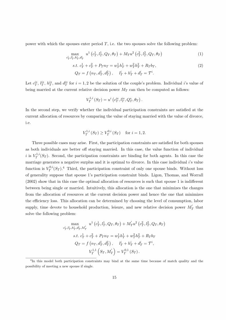
power with which the spouses enter period T , i.e. the two spouses solve the following problem:
maxciT ,liT ,hi
T ,diT
u1(c1T , l
1T , QT , θT
)+MTu
2(c2T , l
2T , QT , θT
)(1)
s.t. c1T + c2T + PTnT = w1Th
1T + w2
Th2T +RT bT , (2)
QT = f(nT , d
1T , d
2T
), liT + hiT + diT = T i.
Let ci∗T , li∗T , hi∗T , and di∗T for i = 1, 2 be the solution of the couple’s problem. Individual i’s value of
being married at the current relative decision power MT can then be computed as follows:
V 1,iT (ST ) = ui
(ci∗T , l
i∗T , Q∗
T , θT).
In the second step, we verify whether the individual participation constraints are satisfied at the
current allocation of resources by comparing the value of staying married with the value of divorce,
i.e.
V 1,iT (ST ) ≥ V 0,i
T (ST ) for i = 1, 2.
Three possible cases may arise. First, the participation constraints are satisfied for both spouses
as both individuals are better off staying married. In this case, the value function of individual
i is V 1,iT (ST ). Second, the participation constraints are binding for both agents. In this case the
marriage generates a negative surplus and it is optimal to divorce. In this case individual i’s value
function is V 0,iT (ST ).
4 Third, the participation constraint of only one spouse binds. Without loss
of generality suppose that spouse 1’s participation constraint binds. Ligon, Thomas, and Worrall
(2002) show that in this case the optimal allocation of resources is such that spouse 1 is indifferent
between being single or married. Intuitively, this allocation is the one that minimizes the changes
from the allocation of resources at the current decision power and hence the one that minimizes
the efficiency loss. This allocation can be determined by choosing the level of consumption, labor
supply, time devote to household production, leisure, and new relative decision power M′T that
solve the following problem:
maxciT ,liT ,hi
T ,diT ,M′T
u1(c1T , l
1T , QT , θT
)+M
′Tu
2(c2T , l
2T , QT , θT
)s.t. c1T + c2T + PTnT = w1
Th1T + w2
Th2T +RT bT
QT = f(nT , d
1T , d
2T
), liT + hiT + diT = T i,
V 1,1T
(ST ,M
′T
)= V 0,1
T (ST ) .
4In this model both participation constraints may bind at the same time because of match quality and the
possibility of meeting a new spouse if single.
15

Let c1∗∗T , l1∗∗T , c2∗∗T , l2∗∗T and M′∗∗ be the solution of this problem. Then if the participation
constraint of spouse 2 is also satisfied the two spouse stay married and the value function of
individual i is
V 1,iT (ST ) = ui
(ci∗∗T , li∗∗T , Q∗∗
T , θT).
Otherwise they divorce and the value function of individual i corresponds to the value of being
single V 0,iT (ST ).
Consider now the case in which individual i enters period T as single. The value function can be
computed using the approach described above with two modifications. First, the relative decision
power is not a state variable but a parameter that is assumed to be identical across couples and will
be estimated. Second, there is no renegotiation. As a consequence, the value function of individual
i corresponds to the value of marriage V 1,iT
(ci∗T , l
i∗T , Q∗
T , θT)if it is greater than the value of staying
single and to the value of staying single V 0,iT (ST ) otherwise.
The household problem has a similar structure in a generic period t < T . The only difference
is that one have to consider the savings decision, the evolution of human capital, and the trend in
match quality.
4 Assumptions on Preferences, Human Capital, Uncertainty, and
Household Production
The estimation of the proposed model requires assumptions about preferences and human capital
accumulation, about the household production functions, and about the uncertainty that charac-
terizes the environment. The next four subsections outline these assumptions.
4.1 Preferences, Household Production, and Human Capital
We will first describe the preferences of an individual who is single. Her preferences depend on
consumption, leisure, and the two household goods. We assume that the corresponding utility
function takes a Cobb-Douglas form for consumption and leisure and it is strongly separable in the
two public goods, i.e.
ui (c, l, Q) =
(cσi l1−σi
)1−γi
1− γi+ αi lnQ.
The parameters γi > 0, σi > 0, and αi > 0 are allowed to differ across gender.
We will now describe the economic meaning of the parameters. The parameter γi captures the
intertemporal aspects of individual preferences. In particular, −1 /γi is individual i’s intertemporal
elasticity of substitution, which measures the willingness to substitute the composite good C =
16

(ci)σi
(T − hi
)1−σi between different periods. The parameter σi captures the intraperiod features
of individual preferences and it measures how individual i allocates her or his resources between
private consumption and leisure. The parameter αi captures the significance of the household
produced good for individual welfare.
The utility function of a married individual is equal to the utility function of an individual who
is single plus the current value of match quality, i.e.
ui (c, l, Q, θ) =c1−γi
1− γi+
l1−σi
1− σi+ α1,i lnQ+ θ.
The value of match quality θ is not observed. As a consequence every increasing transformation of
match quality f (θ) would produced identical results.
We will now describe the household production function. Its functional form has been chosen to
capture three common insights. First, generally the individual welfare increases with the number
of children.5 Second, conditional on the number of children, the amount of home-produced good
should be an increasing function of the time devoted to household production. Third, the amount
of Q that can be produced with a given amount of hours should change if children are present.
For married households we capture these insights using a production function with the following
functional form:
Q = f (n, dm, dw) = (n+ 1)δ1 (dw)δ2+nδ3 (dm)δ4+nδ5 ,
which implies that
lnQ = δ1 ln (n+ 1) + δ2 ln (dw) + δ3n ln (dw) + δ4 ln (dm) + δ5n ln (dm) .
The parameters have a straightforward interpretation. The parameter δ1 measures the percentage
change in Q if a new child is born independently of its quality. δ2 captures the effect of the time
that the woman devotes to household production on Q. δ3 measures the additional effect of the
woman’s hours if the family has children, where the effect is allowed to be positive or negative. δ4
and δ5 have a similar interpretation for the men’s time. Individuals that are not married have the
same functional form for f except that only the domestic labor of the unmarried individual affects
the production of Q.
We can now substitute lnQ in the utility function to understand which preference and pro-
duction function parameters can be identified. The contribution of the goods Q to the individual
welfare can be written in the following way:
αi lnQ = αiδ1 ln (n+ 1) + αiδ2 ln (dw) + αiδ3n ln (dw) + αiδ4 ln (dm) + αiδ5n ln (dm) i = w,m.
5In the empirical part we will consider only households that have two or fewer children. We will therefore avoid
the problem of negative returns to children that may characterized big families.
17
We therefore have the standard result that only the following combinations of preference and
production function paramameters can be identified:
ζ1,i = αiδ1, ζ2,i = αiδ2, ζ3,i = αiδ3, ζ4,i = αiδ4, ζ5,i = αiδ5 i = w,m.
An important component of the model is the accumulation of human capital. In this paper,
it take the form of labor market experience. If an individual works full time during a period,
his experience increases by one year. Instead, if he works part time, his labor market experience
increases by half a year. The stock of human capital depreciates if an individual does not supply
market labor during a period. The accumulated stock of human capital and its depreciation affect
the probability distribution of wages. Individuals with more experience have a wage distribution
with a higher mean. Similarly, individuals who supplied labor during the previous period have
wage offers that are on average higher.
4.2 Sources of Uncertainty
In the model, individuals face four sources of uncertainty: wage shocks, fertility shocks, match
quality shocks, and marriage market shocks. In this subsection we describe how we model them.
In the model the wage process should generate part of the intra-household specialization ob-
served in the data. To that end, we use a wage precess with the following two features. First,
women and men are allowed to have different wage processes. Second, human capital accumulation
has an effect on the wage process of men and women. We incorporate these two features in the
model as follows. We first assume that wit is log-normally distributed with a mean and variance
that differ across gender. Second, we assume that the mean is a linear function of labor market
experience and of a dummy equal to one if the individual worked in the previous period. The wage
process can therefore be written in the following way:
lnwit = ξ1,i + ξ2,iexpt,i + ξ3,iexp
2t,i + ξ4,ilfpt−1,i + ϵt,i,
where ϵt ∼ N(0, σi
ϵ
)and ϵt is assumed to be identically and independently distributed over time.
The coefficient ξ1,i measures the expected wage for an individual with no experience. The parame-
ters ξ2,i and ξ3,i measure the linear and concave effect on wages of an additional year of experience.
The parameter ξ4,i describes the effect of human capital depreciation on the expected wage. An
individual that did not participate in the labor market in the previous period has an expected wage
that is ξ4,i percent lower than the wage of an individual that supplied labor. Here we make the
simplifying assumption that the depreciation is independent of the accumulated stock of human
capital.
18
The fertility process is a second source of intra-household specialization. For computational
reasons, we do not allow individuals to choose the timing and number of children. Instead, we
follow Brien, Lillard, and Stern (2006) and assume that the fertility choices can be characterized
using a statistical process that matches the data. The generalization of the current model to an
environment in which individuals are allowed to choose when to have children is important, but it
is left for future research.
The statistical process for fertility is estimated using a standard probit. The sample employed
to estimate the probit includes married and unmarried women. An observation is a woman/year
and the dependent variable is a dummy variable that takes the value of one if the number of children
in the household increases in the year following the current year. We experimented with two sets of
independent variables. The first set includes marital status, number of existing children, savings,
labor supply, and age and wage of the woman. This specification would enable the woman to have
control over the fertility process. However, it would have the unrealistic property that women that
do not wish to have a child would increase their labor supply and savings with the purpose of
decreasing the fertility rate. For this reason, we decided to restrict the set of independent variables
to marital status, existing children, and the woman’s age. Specifically, we estimate a specification
that includes the following variables: a dummy equal to one if the woman is younger than 25, and
similar dummies if the woman is between the ages of 25 and 29, between the ages of 30 and 34, or
between the ages of 35 and 39; the same dummies interacted with marital status; and a dummy
equal to 1 if the household already has a child. For computational reasons, we limit the number
of children in a household to be smaller than or equal to 2. Table 3 reports the estimates for the
fertility probit. The most important predictor of fertility are marital status and age. Everything
else equal, a married woman between the ages of 25 and 29 has a probit score that is higher by
.695 standard deviations. Evaluated at the mean, this implies that a married woman has a 6.8
percentage point higher probability of having a child during a given year. This effect is large
relative to the overall fertility rate in the sample of 10.1%. The current number of children in the
household is also predictive. Relative to households without children, households with one child
are more likely to give birth to a second child.
Match quality represents a third source for intra-household specialization. As discussed in the
previous section, we model in a reduced form way a framework of learning about match quality.
Specifically, we assume that match quality in period t is perceived to be
θt = θt−1 + tθ∆θ,
where tθ is a positive slope if the household is characterized by a positive trend and negative
otherwise, tθ∆θ is the constant increase or decrease in match quality that affect the household in
19
each period of marriage, and θt−1 = θi, the initial value of match quality, if t − 1 is the year of
marriage. The slope tθ will be estimated, whereas ∆θ will be set equal to the average value of
match quality from which households can initially draw θi, conditional on the initial match quality
being positive. With a given probability pθ, in each period households switch from the current
trend to a trend with opposite sign.
The marriage market is modeled using a simply random search framework. In each period, an
individual who is single meets with probability one a potential spouse. The set of characteristics
that defines the potential spouse are drawn from a uniform distribution which is constructed using
a discretized version of the continuous state variables which will be discussed in the next section.
There is one exception to the assumption that the potential spouse is drawn from a uniform distri-
bution. We assume that an individual draws a potential spouse with similar wealth to capture the
common insight that individuals generally meet partners of similar economic and social extraction.
In practice, we compute the point on the wealth grid that is the closest to the wealth level of the
unmarried individual. We then assume that she can only meet a potential spouse with a wealth
level that is one point below, one point above, or at the same point of the wealth grid.
5 Estimation Implementation
This section discusses the estimation of the model developed in this paper. The model is estimated
using the Simulated Method of Moments (SMM) and data from the 1984-1996 waves of the PSID.
In 1997 the survey was redesigned for biennial data collection. For this reason, data gathered
starting in 1997 are not included.6
To estimate the parameters using the SMM, the model is first simulated to generate an artificial
data set of labor supply, marital status, consumption, and wealth paths. The simulated data
are then used to compute moments such as the divorce hazard rate, the percentage of married
individuals, the average labor supply of married men. These simulated moments are then compared
with the corresponding moments computed using the actual data. The objective of the estimation
is to search for structural parameters that minimize a weighted sum of the distances between the
simulated and data moments. In the estimation we use the inverse of the covariance matrix of
the data moments as a weighting matrix. The covariance matrix is computed using a standard
bootstrap method with 10000 bootstraps.
We will now describe the main aspects of the simulation that is required to compute the sim-
ulated moments. In case of divorce, in the model household wealth must be divided between the
6In 1990, 2,000 latino households were added to the sample. This latino sample was dropped after 1995 and
replaced with a sample of 441 immigrant families in 1997. We exclude both the latino and immigrant samples.
20

spouses. To determine the fraction that is allocated to the wife, we use divorce settlements from the
National Longitudinal Study of the High School Class of 1972 (NLS-72), Fifth Follow-up (1986).
The sample (n=1685) includes all first marriages that ended in legal divorce prior to 1986. The
average percentage of wealth allocated to the wife is 0.496 with a standard deviation of 0.177, where
household wealth is the total net value of all property including the house value and the value of
other real estate. In the simulation we, therefore, assume that wealth is divided equally between
the two spouses.
To deal with households that have income levels below the subsistence level, we introduce
subsidies in the form of the Earned Income Tax Credit (EITC). This program was introduced 1975
and was made more generous over the years. The EITC is a refundable federal income tax credit for
working individuals and families with income below given thresholds. Conditional on the number
of children, there are three income thresholds that determine the amount of the credit. The first
threshold τ1 determines the end of the phase-in part of the EITC: families with income below τ1
receive a credit that is equal to a percentage g1 multiplied by the family income. The second
threshold τ2 establishes the end of the plateau part of the EITC: families with income between τ1
and τ2 receive a constant credit which is equal to the percentage g1 multiplied by the first threshold
τ1. The last threshold τ3 ends the phase-out part of the EITC where families with income between
τ2 and τ3 receive a credit that declines at a rate g2 starting from g1τ1. For instance, for a household
with two children, in 1993, τ1, τ2, and τ3 were equal to $7, 750, $12, 200, and $23, 050, respectively.
The percentages g1 and g2 were set equal to 19.5% and 13.93%.
In the simulation one has to decide which parent receives custody of the children in case of
divorce. According to the United States Census, 58.1% of mothers are the custodial parent. Data
collected from the US Census also indicates that only 54.9% of fathers have either joint custody or
visitation rights. The standard arrangement in case of visitation rights is that the non-custodial
parents can spend 2 weekend days every two weeks with their children. This corresponds to around
15% of time for 54.9% of fathers. To be consistent with these facts, it is assumed that mothers
maintain custody of their children and that children spend 85% of their time with the mother
and the remaining 15% with the father. In the simulation, we implement this by multiplying the
number of children in the production function of a divorced mother by 0.85 and of a divorced father
by 0.15. In addition, the mother pays 85% of the children’s cost and the father the residual part.
To simplify the simulation, it is also assumed that in case of remarriage of one of the two parents,
the children spend 100% of their time with the mother and that the father does not pay any child
cost. This is equivalent to assuming that the utility provided by children to divorced fathers in
case of remarriage is equivalent to the utility provided by the quantity of composite good C that
divorced fathers can purchase with the income they save by not paying the cost of children.
21

The state space has been chosen to reflect the features of the sample that will be used in the
simulation. We start with a description of the grid for the three sources of uncertainty. First,
the continuous distribution of real wages is approximated using the method proposed by Kennan
(2004). He shows that the best discrete approximation F to a given distribution F using the fixed
support points wini=1 is given by
F (wi) =F (wi) + F (wi+1)
2,
where n denotes the number of support points and i indexes each point. In the simulation we set
n equal to 3 and we use as grid points the real wages that corresponds to the 1/6th, 3/6th, and
5/6th point of the empirical distribution. The corresponding grid for women is $2.93, $4.70, and
$7.91. The grid for men is $3.96, $6.60, and $10.72. Dollar values are reported in 1984 dollars.
Second, the grid for children is composed of 3 points, starting with zero children and ending with 2
children. The number of children varies according to the fertility process illustrated in the previous
section. Third, it is assumed that the initial match quality is drawn from a five-point distribution.
The decision variables savings and relative decision power, M , are also discretized. Wealth is
described using an equally-spaced 12-point grid varying between -$75,000 and $200,000 for singles
and between -$150,000 and $400,000 for married individuals. This range is chosen to reflect the
distribution of total wealth minus home equity and the value of vehicles in the PSID, where about
5.2% of households report a wealth level below our range and 4.7% above. We have experimented
with using a larger range for wealth, particularly on the high end, and we have found that few
households choose to accumulate such high levels of wealth. The grid for relative decision power
includes 13 points: 0.000001, 0.05, 0.10, 0.20, ..., 0.80, 0.90, 0.95, and 0.99999. We have tested the
robustness of the simulations with respect to changing the number of grid points for the relative
decision power and we have found that it is important to include a reasonably fine grid. With
a grid that is too coarse, there may be mutually beneficial marriages that do not occur because
the grid does not contain any point within the range of Pareto weights for which the marriage is
sustainable.
The grid for experience requires a separate discussion. This grid can be constructed in two
different ways. A first possibility is to choose a number of points for the grid that is equal to the
number of periods in the simulation. Then in a given year, the individual’s experience increases
by one if she works full time and by half if she works part time. This approach is computationally
demanding since it increases significantly the size of the state space. We therefore adopt a different
strategy that generates similar results. The grid for experience is constructed using a two-point
distribution, 0 and 20 years. Experience then increases according to the following law of motion.
If an individual with 0 experience works full time in a given period, she has a 1 in 20 chances of
22
moving to the high experience state. If she works part time, the probability of moving to the higher
experience level decreases to 1 in 40 changes. Thus, the expected increase in experience for such an
individual is equivalent to the expected increase generated by the first approach. This mechanism
allows us to capture the effect of labor supply on human capital accumulation without using a grid
that makes the simulations excessively time consuming.
The model is simulated for 60 periods. In the first 40 periods individuals make decisions about
marriage, labor supply, consumption, and savings. The remaining 20 years represent the retirement
period, where individuals can only choose consumption and saving. The rate of return on savings
is allowed to change over time. In particular, for 1982-2004 the 20-year municipal bond rate is used
as the relevant rate of return.7 For 2005-2009 the interest rate is assumed to remain unchanged at
the 2004 level.
We solve the problem using backward induction. Consider an arbitrary period. Each individual
enters the period either as single or married. If the individual is single, she draws a potential
spouse from the distribution of available spouses. For this unmarried individual and her potential
spouse, we first evaluate the level of utility associated with being single. We then compute the
level of utility associated with being married this period and with making optimal decisions from
next period onward. The level of utility conditional on marital status is computed by checking
all possible alternatives for consumption, labor supply, time devoted to household production, and
savings, and by selecting the choice that yields the highest level of utility. The two individuals
will choose to marry and the corresponding value of consumption, labor supply, time devoted to
household production, and savings if for both of them the value of being married is higher than
the value of being single.
If two individuals enter the period as married, we follow a similar procedure with the following
exception. The value of being married must first be computed at the value of the relative decision
power with which the two spouses entered the period. We then determine to which of the following
three regimes the couple belongs: (i) both individuals prefer being single; (ii) both individuals
prefer being married; (iii) one individual prefers being single whereas the other is better off as
married. In the first two cases the marital choice is straightforward: in case (i) they stay married
at the current decision power, while in case (ii) they divorce. In the third case, we allow the couple
to renegotiate the current and future allocation of resources. Specifically, we find the allocation
that makes the constrained spouse just indifferent between being single and being married to the
current partner. This goal is achieved by shifting the relative decision power, and accordingly the
allocation, until this indifference condition is satisfied. If at the new allocation both individuals
prefer being married, the couple remains married. Otherwise the two spouses divorce since the
7The rates are obtained from Bloomberg.
23

marriage generates no positive surplus.
It is worth discussing in more details the mechanism by which potential spouses are drawn.
Each individuals is characterized by his own experience, wage, wealth, number of children, relative
decision power, and match quality. For potential spouses, experience and wages are drawn from the
discrete grid described above. Wealth is drawn using a similar approach, but as mentioned earlier
each individual can only draw a potential spouse with a wealth level that is one point below, one
point above, or at the same point in the wealth grid. With regard to children, it is assumed that
single men draw only women with no children. We make this assumption for two reasons. First,
men in the age range considered in our simulations marry mostly women with no children. Second,
in our model men derive utility from children independently of whether the children were conceived
during or before the marriage. This implies that, if we do not make this assumption, single men
search for single women with children to increase their utility after marriage, which is unrealistic.
The initial relative decision power, M , is estimated with the rest of the parameters. Finally, match
quality is drawn from our discrete grid with equal probability for each point.
The solution of the model generates value functions for single and married individuals. The value
functions are then used to simulate the model for the group of individuals available in the 1984 wave
of the PSID that satisfy the selection restrictions mentioned above. For each individual in the 1984
wave we match her experience and number of children to the point of the corresponding grid that
most closely approximates each of the characteristics observed in the data. For married individuals
there are two state variables that are not observed: relative decision power and match quality. We
need to make two assumptions for individuals who are already married in the 1984 wave. First, we
assume that their relative decision power is equivalent to the one that characterizes a newly married
couple. After the first period, their relative decision power is optimally computed. Second, we
assume that their initial match quality is drawn from our grid using a probability distribution that
assigns higher probabilities to positive values of match quality, where the probability is estimated.
Each individual is then simulated 100 times for the period 1984-2034.
We now describe how individuals are followed in the simulation. In the simulation there are
three groups of individuals. The first group includes individuals that are in the 1984 wave and in
1968 lived in one of the households that formed the original 1968 PSID sample. These individuals
are tracked by the PSID even if there is a split-off. There are two main reasons for a split-off: a
child in one of the original families forms her own household; or a couple in the original sample or
one of their children divorces. We will refer to them as tracked individuals. Given the age range
used in this paper, all our tracked individuals are children of families in the original sample. The
second group comprises of individuals that are in the 1984 wave, but are not tracked by the PSID.
If there is a split-off, they vanish from the data set. The third group is composed of individuals
24
that appear in the simulation as potential or actual spouses of the tracked agents. To illustrate the
different treatment in the simulation of these groups, consider the case of a track individual who is
single in the initial period. In this period, she meets a potential spouse. If the couple decides not
to marry, the potential spouse is dropped from the simulation. If the couple marries, the drawn
individual will remain in the simulated sample until the couple chooses to divorce. For individuals
who are initially married, only one of the two individuals is the tracked agent. The other individual
is dropped from the simulation if the household ever decides to divorce.
27 parameters are structurally estimated: the wage parameters (10); the preference parameters
(4); the parameters that determine the effect of children and of the time devoted to household
production on the individual utility (10); the match quality parameters (4); the cost of divoce; the
initial pareto weight; and the probability of meeting a potential spouse if the woman has children.
The risk aversion parameters are set equal to 1 for both men and women. The discount factor is
also assumed to be identical for women and men and equal to 0.99. The remaining parameters
are identified using the following moments. We use 13 wage and labor supply moments: the labor
force participation of single women, single men, married women, and married men; the fraction of
women and of men working at t− 1, but not working at t; the standard deviation of women’s and
men’s wage residuals; the difference between the average wage of women who have between 6 and
19 years of experience and women who have 5 years of experience or less; the difference between
the average wage of women who have 20 years of experience or more and women who have between
6 and 19 years of experience; the same two moments for men. We employ 5 leisure moments: the
average leisure of single women and men; the ratio between the wife’s and husband’s leisure the
first year of marriage for couples with no children; the same moment for couples with children. We
use 8 household production moments: the average hours devoted to household production by single
women with and without children, single men with and without children, married women with and
without children, married men with and without children. Finally, we use 7 marriage and divorce
moments: average years of marriage; marriage hazard with and without children; divorce hazard
with and without children; divorce hazard after one year of marriage; divorce hazard after 3 years
of marriage.
6 Results
This section first presents the estimation results and then uses simulated data obtained employing
the estimated coefficients to evaluate the ability of the model to replicate the patterns observed
in the actual data. For consistency with the PSID survey, tables and figures constructed with the
simulated data only use tracked or married individuals.
25
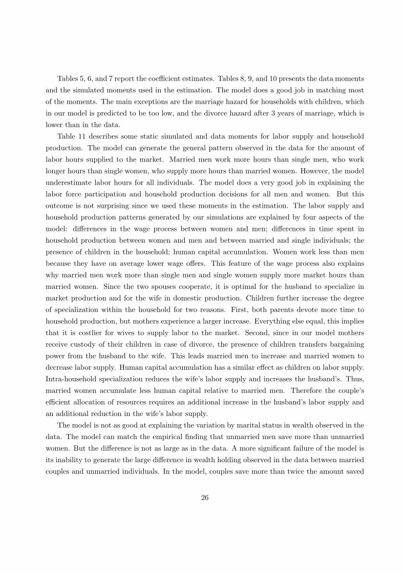
Tables 5, 6, and 7 report the coefficient estimates. Tables 8, 9, and 10 presents the data moments
and the simulated moments used in the estimation. The model does a good job in matching most
of the moments. The main exceptions are the marriage hazard for households with children, which
in our model is predicted to be too low, and the divorce hazard after 3 years of marriage, which is
lower than in the data.
Table 11 describes some static simulated and data moments for labor supply and household
production. The model can generate the general pattern observed in the data for the amount of
labor hours supplied to the market. Married men work more hours than single men, who work
longer hours than single women, who supply more hours than married women. However, the model
underestimate labor hours for all individuals. The model does a very good job in explaining the
labor force participation and household production decisions for all men and women. But this
outcome is not surprising since we used these moments in the estimation. The labor supply and
household production patterns generated by our simulations are explained by four aspects of the
model: differences in the wage process between women and men; differences in time spent in
household production between women and men and between married and single individuals; the
presence of children in the household; human capital accumulation. Women work less than men
because they have on average lower wage offers. This feature of the wage process also explains
why married men work more than single men and single women supply more market hours than
married women. Since the two spouses cooperate, it is optimal for the husband to specialize in
market production and for the wife in domestic production. Children further increase the degree
of specialization within the household for two reasons. First, both parents devote more time to
household production, but mothers experience a larger increase. Everything else equal, this implies
that it is costlier for wives to supply labor to the market. Second, since in our model mothers
receive custody of their children in case of divorce, the presence of children transfers bargaining
power from the husband to the wife. This leads married men to increase and married women to
decrease labor supply. Human capital accumulation has a similar effect as children on labor supply.
Intra-household specialization reduces the wife’s labor supply and increases the husband’s. Thus,
married women accumulate less human capital relative to married men. Therefore the couple’s
efficient allocation of resources requires an additional increase in the husband’s labor supply and
an additional reduction in the wife’s labor supply.
The model is not as good at explaining the variation by marital status in wealth observed in the
data. The model can match the empirical finding that unmarried men save more than unmarried
women. But the difference is not as large as in the data. A more significant failure of the model is
its inability to generate the large difference in wealth holding observed in the data between married
couples and unmarried individuals. In the model, couples save more than twice the amount saved
26

by unmarried individuals. But the difference in wealth by marital status is far from the difference
observed in the PSID.
We will now evaluate the ability of the model to explain the evolution of labor supply and time
devoted to household production during a transition into and out of marriage. Figure 19 describes
the labor supply pattern for women as they enter marriage. As before, an index is used where 0
denotes the first year of a transition between marital states. In the PSID, women’s labor supply
decreases starting one-two years prior to marriage and continues to gradually decrease during the
first five years of marriage. Moreover, at the time of marriage women’s labor supply is between
the average labor supply of married women and the average labor supply of single women. The
model can generate the pattern observed in the data starting from the year in which the woman
marries. In the simulations, in the year of marriage women supply on average an amount of labor
that is between the labor hours supplied by single women and married women. After women
enter marriage, in the model their labor supply declines steadily until the fifth year of marriage
when their labor hours reach the level of the average married woman. The model cannot replicate
the decline in labor hours in the one-two years that precede marriage. This outcome should be
expected since in our model individuals meet and immediately choose whether to marry. There is
therefore no dating period in which the two potential spouses may decide to start preparing for
marriage by changing their labor supply decisions. The gradual decline of labor supply for married
women after marriage is explained by three features of our model: the presence of children; the
differential accumulation of human capital between wife and husband; the absence of commitment.
During these years married women tend to work less and less as they increase the time devoted to
household production and increase their bargaining power in the marriage. This causes married
women to accumulate less human capital relative to married men. For the household, it is therefore
optimal to further increase specialization by reducing the wife’s labor supply and by increasing the
husband’s hours of work even more. The lack of commitment produces a more gradual decline in
the amount of hours supplied by wives. To see this note that married women know that with some
probability the marriage will end, in which case the accumulated human capital will be important.
Conditional on children, the probability of divorce depends on the level of match quality. In
our model the marriages that survive are the ones with an upward trend in match quality or,
equivalently, marriages where the spouses learn over time that the quality of their match is high.
In this marriages, the spouses increase gradually the degree of specialization, which explain the
gradual decline in labor supply of women. Figures 21 and 23 show the simulation results for labor
force participation and labor supply conditional on working. Figure 25 presents the simulation
results for household production before and during marriage. The model is able to replicate the
patterns observed in the data at the time of marriage and after.
27

Figure 20 describes the labor supply behavior of men generated by the model as they enter
marriage. Similarly to the pattern observed in the PSID, in the model men increase their labor
hours at the time of marriage. However, the model cannot generate the gradual increase in labor
supply after men enter marriage. Married men move to the higher level of labor supply and remain
there during the years they stay married.
Figure 27 describes women’s labor supply before and after divorce. Both this figure and the
analogous figure obtained using the PSID describe a steady increase in labor supply beginning
several years prior to divorce. In the model this behavior is explained by two types of married
couples: couples with a downward trend in match quality and couples in which the wife experiences
a high wage offer and therefore increases her labor supply. To provide the intuition underlying
this result, consider first a couple with a downward trend in match quality. In this case, the
probability of divorce increases over time. It is therefore optimal for the spouses to reduce the
degree of intra-household specialization, which explains the gradual increase in the wife’s labor
supply. Consider now a couple in which the wife receives a good wage offer. In this case, she will
increase her labor supply and reduce the time spend in household production. As a consequence,
the marriage produces a lower amount of public good, which increases the probability of divorce.
As a consequence, it is optimal for the pair to reduce the degree of specialization, which increases
even more the probability of divorce. Figures 29 and 30 show the simulation results for labor supply
conditional on working and labor force participation.
Figure 28 describes the labor supply pattern for men before and after divorce. This Figure
should be compared to Figure 16 which describes the same pattern in the PSID. In the PSID, before
divorce men work about the same amount of hours as the average married man. In the simulation
labor supply displays a similar pattern. In the PSID, after divorce men decrease gradually their
labor supply. In the model, similarly to what is observed in the data, men experience a drop in
labor supply the year of the divorce. But then increase their labor hours, which is not the pattern
displayed by the data.
7 Policy Evaluation
In this section we use the estimated model to evaluate the effect of two policies on the labor
supply and household production decisions of low-income households. The first one consists in the
removal of the EITC program. The second policy replaces the EITC with a program that is meant
to reduce the labor supply disincentives that are implicit in the EITC. The alternative program has
the following features. A family with an income below Y receives, independently of labor supply
decisions, a fixed subsidy equal to the percentage paid by the EITC program in its phase-in part,
28
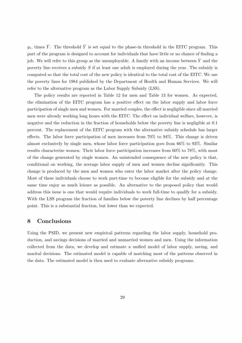
g1, times Y . The threshold Y is set equal to the phase-in threshold in the EITC program. This
part of the program is designed to account for individuals that have little or no chance of finding a
job. We will refer to this group as the unemployable. A family with an income between Y and the
poverty line receives a subsidy S if at least one adult is employed during the year. The subsidy is
computed so that the total cost of the new policy is identical to the total cost of the EITC. We use
the poverty lines for 1984 published by the Department of Health and Human Services. We will
refer to the alternative program as the Labor Supply Subsidy (LSS).
The policy results are reported in Table 12 for men and Table 13 for women. As expected,
the elimination of the EITC program has a positive effect on the labor supply and labor force
participation of single men and women. For married couples, the effect is negligible since all married
men were already working long hours with the EITC. The effect on individual welfare, however, is
negative and the reduction in the fraction of households below the poverty line is negligible at 0.1
percent. The replacement of the EITC program with the alternative subsidy schedule has larger
effects. The labor force participation of men increases from 70% to 94%. This change is driven
almost exclusively by single men, whose labor force participation goes from 66% to 93%. Similar
results characterize women. Their labor force participation increases from 60% to 78%, with most
of the change generated by single women. An unintended consequence of the new policy is that,
conditional on working, the average labor supply of men and women decline significantly. This
change is produced by the men and women who enter the labor market after the policy change.
Most of these individuals choose to work part-time to become eligible for the subsidy and at the
same time enjoy as much leisure as possible. An alternative to the proposed policy that would
address this issue is one that would require individuals to work full-time to qualify for a subsidy.
With the LSS program the fraction of families below the poverty line declines by half percentage
point. This is a substantial fraction, but lower than we expected.
8 Conclusions
Using the PSID, we present new empirical patterns regarding the labor supply, household pro-
duction, and savings decisions of married and unmarried women and men. Using the information
collected from the data, we develop and estimate a unified model of labor supply, saving, and
marital decisions. The estimated model is capable of matching most of the patterns observed in
the data. The estimated model is then used to evaluate alternative subsidy programs.
29

References
Andres, Erosa, Luisa Fuster, and Diego Restuccia. 2005. “A Quantitative Theory of the Gender
Gap in Wages.” Manuscript.
Attanasio, Orazio, and Jose-Victor Rios-Rull. 2000. “Consumption smoothing in island economies:
Can public insurance reduce welfare?” European Economic Review 44 (7): 1225–1258 (June).
Blundell, Richard, Pierre-Andre Chiappori, Thierry Magnac, and Costas Meghir. 2007. “Collective
Labour Supply: Heterogeneity and Non-Participation.” Review of Economic Studies 74:417–
445.
Browning, Martin, Francois Bourguignon, Pierre-Andre Chiappori, and Valerie Lechene. 1994.
“Income and outcomes: a structural model of intrahousehold allocation.” Journal of Political
Economy 102:1067–96.
Casanova, Maria. 2010. “Happily Together: A Structural Model of Couples’ Joint Retirement
Choices.” Working Paper, UCLA.
Chiappori, Pierre Andre. 1988. “Rational household labor supply.” Econometrica 56:63–89.
. 1992. “Collective labor supply and welfare.” Journal of Political Economy 100:437–467.
Chiappori, Pierre Andre, Bernard Fortin, and Guy Lacroix. 2002. “Marriage Market, Divorce
Legislation, and Household Labor Supply.” Journal of Political Economy 110 (1): pp. 37–72.
Donni, Olivier. 2004. “A Collective Model of Household Behavior with Private and Public Goods:
Theory and Some Evidence from U.S. Data.” DELTA Working Papers.
Fernandez, Raquel, and Joyce Cheng Wong. 2011. “The Disappearing Gender Gap: The Impact of
Divorce, Wages, and Preferences on Education Choices and Women’s Work.” NBER Working
Papers, no. 17508.
Gemici, Ahu. 2011. “Family Migration and Labor Market Outcomes.” Working Paper, NYU.
Gemici, Ahu, and Steve Laufer. 2011. “Marriage and Cohabitation.” Working Paper, NYU.
Guner, Nezih, and John Knowles. 2003. “A Quantitative Theory of the Gender Gap in Wages.”
Manuscript.
Heckman, James J., and Thomas E. Macurdy. 1980. “A Life Cycle Model of Female Labour
Supply.” The Review of Economic Studies 47 (1): pp. 47–74.
Jones, Larry E., Rodolfo E. Manuelli, and Ellen R. McGrattan. 2003. “Why are married women
working so much?” no. 317.
Kennan, John. 2004. “A Note on Approximating Distribution Functions.” Manuscript.
30

Kocherlakota, Narayana R. 1996. “Implications of Efficient Risk Sharing without Commitment.”
Review of Economic Studies 63:595–609.
Ligon, Ethan, Jonathan P Thomas, and Tim Worrall. 2002. “Informal Insurance Arrangements
with Limited Commitment: Theory and Evidence from Village Economies.” Review of Eco-
nomic Studies 69:209–44.
Lundberg, Shelly, Richard Startz, and Steven Stillman. 2003. “The retirement-consumption
puzzle: a marital bargaining approach.” Journal of Public Economics 87 (56): 1199 – 1218.
Manser, Marilyn, and Murray Brown. 1980. “Marriage and Household Decision-Making: A
Bargaining Analysis.” International Economic Review 21 (1): pp. 31–44.
Marcet, Albert, and RamonMarimon. 1992. “Communication, commitment, and growth.” Journal
of Economic Theory 58 (2): 219–249 (December).
. 1998. “Recursive Contracts.” Working Paper, European University Institute, no. eco98/37.
Mazzocco, Maurizio. 2004. “Saving, Risk Sharing, and Preferences for Risk.” The American
Economic Review 94 (4): pp. 1169–1182.
. 2007. “Household Intertemporal Behaviour: A Collective Characterization and a Test of
Commitment.” Review of Economic Studies 74:857–895.
McElroy, Marjorie B., and Mary Jean Horney. 1981. “Nash-bargained household decisions: toward
a generalization of the theory of demand.” International Economic Review 22:333–349.
Olivetti, Claudia. 2006. “Changes in Women’s Hours of Market Work: The Role of Returns to
Experience.” Review of Economic Dynamics 9 (4): 557–587 (October).
Rios-Rull, Jose-Victor, Jacob Short, and Ferdinando Regalia. 2010. “What Accounts for the
Increase in the Number of Single Households?” no. 995.
Tartari, Melissa. 2007. “Divorce and Cognitive Achievement of Children.” Working Paper, Yale
University.
Thomas, Duncan. 1990. “Intra-household resource allocation: An inferential approach.” Journal
of Human Resources 25:635–664.
van der Klaauw, Wilbert, and Kenneth I. Wolpin. 2008. “Social security and the retirement and
savings behavior of low-income households.” Journal of Econometrics 145 (1-2): 21–42 (July).
Voena, Alessandra. 2011. “Yours, Mine and Ours: Do Divorce Laws Affect the Intertemporal
Behavior of Married Couples?” Working Paper, Stanford University.
31

B. Tables
Table 1: PSID Descriptive Statistics
Mean SD
Marital Status and Transitions:
percentage married .79 (.41)
marriage hazard .101 (.392)
divorce hazard .030 (.169)
Labor Force Participation:
single women .91 (.26)
single men .96 (.18)
married women .66 (.39)
married men .98 (.15)
Annual Hours Worked if Working:
single women 1861 (669)
single men 2095 (711)
married women 1660 (736)
married men 2312 (622)
Annual Hours Spent on Household Production:
single women 604 (482)
single men 372 (349)
married women 1287 (729)
married men 366 (351)
Note: The PSID is a longitudinal study of a representative sample of U.S. individuals. The sample is from the
1968-1996 waves and the 1984, 1989 and 1994 Wealth Supplement Files. The Latino and Immigrant Samples have
been excluded along with the 1968 low-income Census oversample. The sample is restricted to include only household
heads and wives, not sons, daughters or other household members, unless they have started their own household.
After these exclusions there are 29,594 total individual-year observations, or, about 2000 individual-year observations
per year. Each survey wave records extensive individual-level information on labor supply and wages. Annual hours
worked is constructed as the typical number of hours worked at each of up to three jobs multiplied by the number of
weeks during the year worked at each job. Wages are calculated as annual individual labor market income divided by
total annual hours worked. After-tax wages are adjusted for federal and state income tax using the NBER’s TAXSIM
using household income, year, state of residence, marital status, and number of children.
32

Table 2: Average Wealth Levels in the PSID
married couples $49,732
unmarried individuals $11,161
married couples the year before divorce $18,471
individuals the year before marriage $11,499
just married couples $19,798
just divorced individuals $8,385
Note: The transitions are described over the last year. For example, “married couples just before divorce” arecurrently married but will not be married next year and “just married couples” are currently married but were notmarried last year. The wealth measure excludes wealth in housing and cars.
Table 3: Estimates of Fertility Process (Probit)
dependent variable
25 ≤ age < 29 -.114(.081)
29 ≤ age < 34 .105(.083)
35 ≤ age < 39 .261(.088)
age < 25 and married .675(.065)
25 ≤ age < 29 and married .695(.063)
30 ≤ age < 34 and married .507(.068)
35 ≤ age < 39 and married .067(.077)
one child 0.175(.032)
constant -1.486(.057)
n 11180
Note: The dependent variable is a dummy equal to one if during the current year the household gives birthto a child.
33

Table 4: Annual Cost of Children, CEX 1980-1996
dependent variable
cost for first child 486.0(16.2)
cost for second child 370.8(17.0)
cost for additional children 287.3(9.98)
Note: The dependent variable is a measure of annual expenditure that includes food at home, child care,boy’s clothing and shoes, girl’s clothing and shoes, and infant clothing. The sample includes households withthe head with ages 20 to 40. All dollar values have been deflated to reflect year 1984 dollars. Coefficientsfor after tax income, age of the household head, education of the household head, race and marital statusare omitted. The regression includes 29,961 observations and the R2 is .36.
Table 5: Estimates for the Wage Processes
Women
experience 0.622experience2 -0.021dummy if not working at t− 1 -0.424constant 1.351standard deviation 4.861
Men
experience 0.409experience2 -0.011dummy if not working at t− 1 -0.548constant 1.636standard deviation 5.452
Table 6: Estimates of the Public Good Parameters
Women’s Preferences
children 0.323woman’s household time 0.106man’s household time 0.0001woman’s household time X children 0.100man’s household time X children 0.0000
Men’s Preferences
children 2.011man’s household time 0.929woman’s household time 0.478man’s household time X children 0.0002woman’s household time X children 0.415
34

Table 7: Estimates of the Remaining Parameters
Woman’s leisure parameter 0.698Man’s leisure parameter 0.698Initial probability of an upward trend 0.45Trend in match quality 2.301Probability of changing trend 0.12Probability a married couple draws an initial negative match quality 0.09Initial Pareto weight 0.28Prob a woman meets a potential spouse if kids 0.33Cost of divorce 28,543
Table 8: Moments Used in EstimationData Simulation
Wage and Labor Supply Moments:
LFP of single women 0.910 0.891
LFP of single men 0.960 0.967
LFP of married women 0.662 0.693
LFP of married men 0.983 0.997
Fraction of women working at t-1 not working at t 0.055 0.057
Fraction of men working at t-1 not working at t 0.009 0.011
Standard deviation of women’s wage residuals 2.880 3.028
Standard deviation of men’s wage residuals 3.483 2.744
E [wwt |5 ≤ Experience < 20 ]− E [ww
t |Experience < 5 ] 1.876 3.689
E [wwt |Experience ≥ 20 ]− E [ww
t |5 ≤ Experience < 20 ] 0.154 3.528
E [wmt |5 ≤ Experience < 20 ]− E [wm
t |Experience < 5 ] 2.184 3.583
E [wmt |Experience ≥ 20 ]− E [wm
t |5 ≤ Experience < 20 ] 0.159 1.227
35

Table 9: Moments Used in EstimationData Simulation
Leisure Moments:
Average leisure of single women 2,843 2,577
Average leisure of single men 2,779 2,538
Ratio wife’s to husb’s leisure 1st year of mar, no kids 1.160 0.996
Ratio wife’s to husb’s leisure 1st year of mar, with kids 1.144 1.016
Household Production Moments:
Average hours on hous prod by single women no kids 473 408
Average hours on hous prod by single men no kids 368 357
Average hours on hous prod by married women no kids 788 756
Average hours on hous prod by married men no kids 350 367
Average hours on hous prod by single women with kids 715 729
Average hours on hous prod by single men with kids 449 357
Average hours on hous prod by married women with kids 1357 1061
Average hours on hous prod by married men with kids 368 364
Table 10: Moments Used in EstimationData Simulation
Marriage Moments:
Years of marriage 7.475 7.427
Marriage hazard no kids 0.100 0.094
Marriage hazard with kids 0.102 0.054
Divorce Moments:
Divorce hazard no kids 0.041 0.035
Divorce hazard with kids 0.015 0.016
Divorce hazard after 1 year of marriage 0.072 0.091
Divorce hazard after 3 years of marriage 0.060 0.013
36

Table 11: Simulation ResultsData Simulation
Annual Hours of Work if Working:single women 1861.3 2125.3single men 2095.6 2301.3married women 1660.2 1761.8married men 2312.3 2388.6
Labor Force Participation:single women 0.910 0.895single men 0.960 0.963married women 0.662 0.693married men 0.983 0.997
Household Production without Childrensingle women 473.1 407.7single men 368.4 356.7married women 787.7 755.5married men 350.7 366.9
Household Production with Childrensingle women 715.0 728.9single men 449.2 356.7married women 1357.2 1060.9married men 368.7 364.1
Wealthunmarried women 8,180 9,198unmarried men 14,149 10,228married couples 49,732 21,276
Table 12: Policy Results: Men
No Subsidy EITC LSSMen b. Poverty LineLFP 0.72 0.70 0.94Cond. Labor Supply 2306.8 2298.7 2088.6Welfare -3990.4 -3990.0 -3989.8Single Men b. Poverty LineLFP 0.67 0.66 0.93Cond. Labor Supply 2286.2 2277.4 2031.0Welfare -4001.9 -4000.8 -4000.5Married Men b. Poverty LineLFP 0.996 0.993 0.994Cond. Labor Supply 2395.2 2394.8 2391.0Welfare -3917.5 -3921.1 -3914.3% Households b. Poverty LineFraction below 10.6 10.7 10.1
37

Table 13: Policy Results: Women
No Subsidy EITC LSSWomen b. Poverty LineLFP 0.61 0.60 0.78Cond. Labor Supply 2293.2 2286.9 2105.8Welfare -3949.0 -3947.4 -3948.6Single Women b. Poverty LineLFP 0.64 0.63 0.83Cond. Labor Supply 2302.6 2295.8 2113.1Welfare -3955.0 -3952.2 -3952.8Married Women b. Poverty LineLFP 0.16 0.16 0.19Cond. Labor Supply 1843.8 1840.7 1748.2Welfare -3875.9 -3871.8 -3873.4% Households b. Poverty LineFraction below 10.6 10.7 10.1
38

Figure 1: PSID 1968-1996, Women’s Labor Supply Before and During Marriage.
1000
1200
1400
1600
1800
Annu
al W
ork H
ours
−5 −4 −3 −2 −1 0 1 2 3 4 5Years Relative To Marriage
Transition SampleNot MarriedMarried − Weighted
Women’s Labor Supply Before and During MarriagePSID 1968−1996
Figure 2: PSID 1968-1996, Men’s Labor Supply Before and During Marriage.
1900
2000
2100
2200
2300
2400
Annu
al W
ork H
ours
−5 −4 −3 −2 −1 0 1 2 3 4 5Years Relative To Marriage
Transition SampleNot MarriedMarried − Weighted
Men’s Labor Supply Before and During MarriagePSID 1968−1996
39
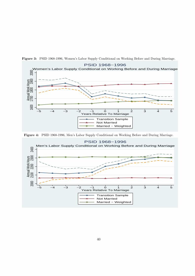
Figure 3: PSID 1968-1996, Women’s Labor Supply Conditional on Working Before and During Marriage.
1600
1700
1800
1900
2000
Annu
al W
ork H
ours
−5 −4 −3 −2 −1 0 1 2 3 4 5Years Relative To Marriage
Transition SampleNot MarriedMarried − Weighted
Women’s Labor Supply Conditional on Working Before and During MarriagePSID 1968−1996
Figure 4: PSID 1968-1996, Men’s Labor Supply Conditional on Working Before and During Marriage.
2000
2100
2200
2300
2400
Annu
al W
ork H
ours
−5 −4 −3 −2 −1 0 1 2 3 4 5Years Relative To Marriage
Transition SampleNot MarriedMarried − Weighted
Men’s Labor Supply Conditional on Working Before and During MarriagePSID 1968−1996
40
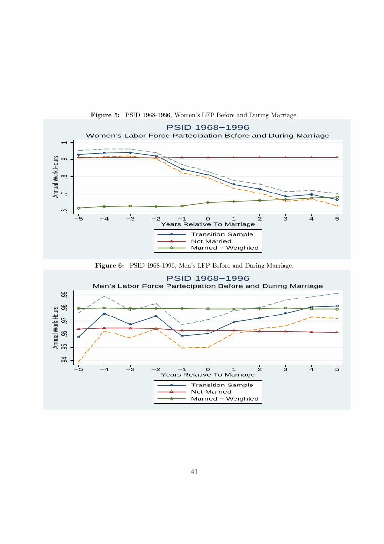
Figure 5: PSID 1968-1996, Women’s LFP Before and During Marriage.
.6.7
.8.9
1An
nual
Work
Hou
rs
−5 −4 −3 −2 −1 0 1 2 3 4 5Years Relative To Marriage
Transition SampleNot MarriedMarried − Weighted
Women’s Labor Force Partecipation Before and During MarriagePSID 1968−1996
Figure 6: PSID 1968-1996, Men’s LFP Before and During Marriage.
.94.95
.96.97
.98.99
Annu
al W
ork H
ours
−5 −4 −3 −2 −1 0 1 2 3 4 5Years Relative To Marriage
Transition SampleNot MarriedMarried − Weighted
Men’s Labor Force Partecipation Before and During MarriagePSID 1968−1996
41
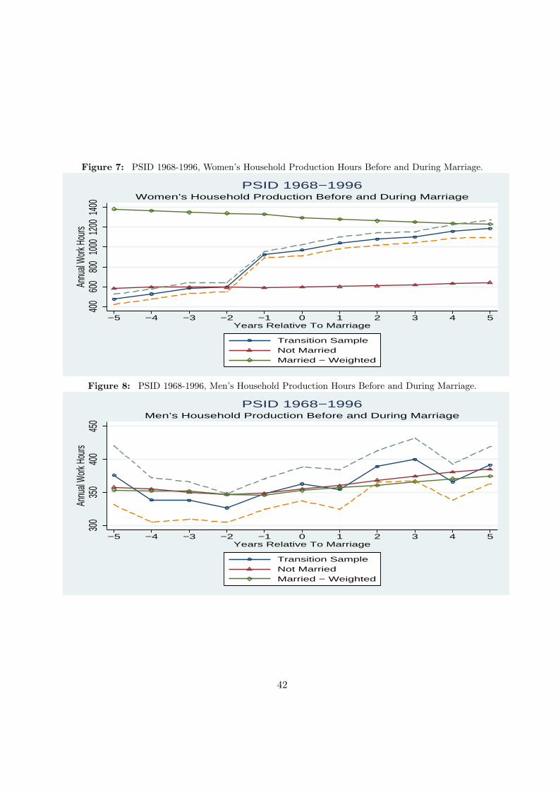
Figure 7: PSID 1968-1996, Women’s Household Production Hours Before and During Marriage.
400
600
800
1000
1200
1400
Annu
al W
ork H
ours
−5 −4 −3 −2 −1 0 1 2 3 4 5Years Relative To Marriage
Transition SampleNot MarriedMarried − Weighted
Women’s Household Production Before and During MarriagePSID 1968−1996
Figure 8: PSID 1968-1996, Men’s Household Production Hours Before and During Marriage.
300
350
400
450
Annu
al W
ork H
ours
−5 −4 −3 −2 −1 0 1 2 3 4 5Years Relative To Marriage
Transition SampleNot MarriedMarried − Weighted
Men’s Household Production Before and During MarriagePSID 1968−1996
42

Figure 9: PSID 1968-1996, Women’s LS Before and After First Birth.
800
1000
1200
1400
1600
1800
Annu
al Ho
urs
−5 −4 −3 −2 −1 0 1 2 3 4 5Years Relative To First Birth
Transition SampleNo kids − WeightedKids − Weighted
Before and After First BirthWomen: Labor Hours
Figure 10: PSID 1968-1996, Men’s LS Before and After First Birth.
2000
2100
2200
2300
Annu
al Ho
urs
−5 −4 −3 −2 −1 0 1 2 3 4 5Years Relative To First Birth
Transition SampleNo kids − WeightedKids − Weighted
Before and After First BirthMen: Labor Hours
43

Figure 11: PSID 1968-1996, LS of Women with no Children.
1500
1600
1700
1800
1900
2000
Annu
al Ho
urs
−5 −4 −3 −2 −1 0 1 2 3 4 5Years Relative To Marriage
Transition SampleSingle − WeightedMarried − Weighted
Before and During MarriageWomen Without Children: Labor Hours
Figure 12: PSID 1968-1996, LS of Men with no Children.
1800
1900
2000
2100
2200
2300
Annu
al Ho
urs
−5 −4 −3 −2 −1 0 1 2 3 4 5Years Relative To Marriage
Transition SampleSingle − WeightedMarried − Weighted
Before and During MarriageMen Without Children: Labor Hours
44

Figure 13: PSID1968-1996, Residual LS of Women without Children.
020
040
060
080
0An
nual
Hours
−5 −4 −3 −2 −1 0 1 2 3 4 5Years Relative To Marriage
Transition SampleSingle − WeightedMarried − Weighted
Before and During MarriageWomen Without Children: Labor Hours
Figure 14: PSID 1968-1996, Residual LS of Men without Children.
−200
−100
010
020
0An
nual
Hours
−5 −4 −3 −2 −1 0 1 2 3 4 5Years Relative To Marriage
Transition SampleSingle − WeightedMarried − Weighted
Before and During MarriageMen With Children: Labor Hours
45

Figure 15: PSID 1968-1996, Women’s Labor Supply Before and After Divorce.
1000
1200
1400
1600
1800
Annu
al W
ork H
ours
−5 −4 −3 −2 −1 0 1 2 3 4 5Years Relative To Divorce
Transition SampleNot MarriedMarried − Weighted
Women’s Labor Supply Before and After DivorcePSID 1968−1996
Figure 16: PSID 1968-1996, Men’s Labor Supply Before and After Divorce.
1900
2000
2100
2200
2300
2400
Annu
al W
ork H
ours
−5 −4 −3 −2 −1 0 1 2 3 4 5Years Relative To Divorce
Transition SampleNot MarriedMarried − Weighted
Men’s Labor Supply Before and After DivorcePSID 1968−1996
46

Figure 17: PSID 1968-1996, Women’s Household Production Before and After Divorce.
600
800
1000
1200
1400
Annu
al W
ork H
ours
−5 −4 −3 −2 −1 0 1 2 3 4 5Years Relative To Divorce
Transition SampleNot MarriedMarried − Weighted
Women’s Household Production Before and After DivorcePSID 1968−1996
Figure 18: PSID 1968-1996, Men’s Household Production Before and After Divorce.
250
300
350
400
450
500
Annu
al W
ork H
ours
−5 −4 −3 −2 −1 0 1 2 3 4 5Years Relative To Divorce
Transition SampleNot MarriedMarried − Weighted
Men’s Household Production Before and After DivorcePSID 1968−1996
47

Figure 19: Simulation, Women’s Labor Supply Before and During Marriage.
1800
1900
2000
2100
2200
Annu
al W
ork H
ours
−5 −4 −3 −2 −1 0 1 2 3 4 5Years Relative To Marriage
Transition SampleNot MarriedMarried − Weighted
Women’s Labor Supply Before and During MarriageSIMULATED DATA
Figure 20: Simulation, Men’s Labor Supply Before and During Marriage.
2250
2300
2350
2400
Annu
al W
ork H
ours
−5 −4 −3 −2 −1 0 1 2 3 4 5Years Relative To Marriage
Transition SampleNot MarriedMarried − Weighted
Men’s Labor Supply Before and During MarriageSIMULATED DATA
48

Figure 21: Simulation, Women’s LFP Before and During Marriage.
.75.8
.85.9
Annu
al W
ork H
ours
−5 −4 −3 −2 −1 0 1 2 3 4 5Years Relative To Marriage
Transition SampleNot MarriedMarried − Weighted
Women’s Labor Force Participation Before and During MarriageSIMULATED DATA
Figure 22: Simulation, Men’s Labor Supply Before and During Marriage.
.95.96
.97.98
.991
Annu
al W
ork H
ours
−5 −4 −3 −2 −1 0 1 2 3 4 5Years Relative To Marriage
Transition SampleNot MarriedMarried − Weighted
Men’s Labor Force Participation Before and During MarriageSIMULATED DATA
49

Figure 23: Simulation, Women’s Labor Supply Conditional on Working Before and During Marriage.
2250
2300
2350
2400
Annu
al W
ork H
ours
−5 −4 −3 −2 −1 0 1 2 3 4 5Years Relative To Marriage
Transition SampleNot MarriedMarried − Weighted
Women’s Labor Supply Conditional on Working Before and During MarriageSIMULATED DATA
Figure 24: Simulation, Men’s Labor Supply Conditional on Working Before and During Marriage.
2250
2300
2350
2400
Annu
al W
ork H
ours
−5 −4 −3 −2 −1 0 1 2 3 4 5Years Relative To Marriage
Transition SampleNot MarriedMarried − Weighted
Men’s Labor Supply Conditional on Working Before and During MarriageSIMULATED DATA
50

Figure 25: Simulation, Women’s Household Production Before and During Marriage.
600
700
800
900
1000
Annu
al W
ork H
ours
−5 −4 −3 −2 −1 0 1 2 3 4 5Years Relative To Marriage
Transition SampleNot MarriedMarried − Weighted
Women’s Household Production Before and During MarriageSIMULATED DATA
Figure 26: Simulation, Men’s Household Production Before and During Marriage.
350
400
450
Annu
al W
ork H
ours
−5 −4 −3 −2 −1 0 1 2 3 4 5Years Relative To Marriage
Transition SampleNot MarriedMarried − Weighted
Men’s Household Production Before and During MarriageSIMULATED DATA
51

Figure 27: Simulation, Women’s Labor Supply Before and After Divorce.
1600
1800
2000
2200
2400
Annu
al W
ork H
ours
−5 −4 −3 −2 −1 0 1 2 3 4 5Years Relative To Divorce
Transition SampleNot MarriedMarried − Weighted
Women’s Labor Supply Before and After DivorceSIMULATED DATA
Figure 28: Simulation, Men’s Labor Supply Before and After Divorce.
2300
2320
2340
2360
2380
2400
Annu
al W
ork H
ours
−5 −4 −3 −2 −1 0 1 2 3 4 5Years Relative To Divorce
Transition SampleNot MarriedMarried − Weighted
Men’s Labor Supply Before and After DivorceSIMULATED DATA OF PSID 1982−1996
52

Figure 29: Simulation, Women’s Conditional Labor Supply Before and After Divorce.
2280
2300
2320
2340
2360
2380
Annu
al W
ork H
ours
−5 −4 −3 −2 −1 0 1 2 3 4 5Years Relative To Divorce
Transition SampleNot MarriedMarried − Weighted
Women’s Labor Supply Conditional on Working Before and After DivorceSIMULATED DATA
Figure 30: Simulation, Women’s Labor Force Participation Before and After Divorce.
.75.8
.85.9
.95An
nual
Work
Hou
rs
−5 −4 −3 −2 −1 0 1 2 3 4 5Years Relative To Divorce
Transition SampleNot MarriedMarried − Weighted
Women’s Labor Force Participation Before and After DivorceSIMULATED DATA
53