Labor Supply on the

US Professional Golfers’ Association Tour Bruce K. Johnsona

John J. Perryb a Corresponding author Centre College, 600 W. Walnut Street, Danville, KY 40422, bruce.johnson@centre.edu , office: (859) 238-5255, fax: (859) 238-5774 b Centre College, 600 W. Walnut Street, Danville, KY 40422, john.perry@centre.edu, The authors thank William R. Johnson, Robert E. Martin, Michael J. Rizzo, Thomas Rhoads, and anonymous referees for their comments.

ABSTRACT

This paper estimates a labor supply model for professional golfers with a systems

approach in which the number and quality of tournaments played, performance, and

expected wage are endogenous. The core finding of this paper is that golfers play fewer

tournaments as their expected wage increases, implying a backward bending labor supply

curve. The estimated labor supply elasticity is -0.088. This finding is in line with existing

literature and is generally robust. The systems approach employed yields other insights

with respect to the expected wage of golfers, the quality of tournaments golfers play, and

the performance of golfers, in addition to the labor supply.

Keywords: Golf, labor supply, backward-bending, PGA

JEL Classification: J01, J22, J44, L83

I. Introduction

The distribution of weekly hours worked has been described as “quite lumpy,

with a substantial fraction of workers reporting usual weekly hours of precisely 40.”

(Farber, 2005, p. 47). This may be because most workers do not have the freedom to vary

their work time and may be why most estimates of male labor supply elasticity have

clustered around zero. Economists have developed some small data sets on labor market

behavior for people free to set their own work hours. Oettinger (1999) found an upward

sloping supply curve for baseball-stadium vendors. Fehr and Goette (2007) estimated an

upward sloping labor supply for Zurich bicycle messengers. Camerer et al. (1997) and

Chou (2000) found backward-bending supply curves for taxi drivers in New York City

and Singapore, respectively. Using a different model, Farber (2005) found upward

sloping labor supply curves for New York City taxi drivers.

Professional golf offers another source of data for workers who can determine

their own amount of labor supplied. Economists have long mined the rich lode of data

from sports labor markets to test important hypotheses in labor economics. As Kahn

(2000) has noted, professional sports offer the only research setting in labor economics in

which we know the name, face, compensation, life history, and performance of every

worker. But most studies of sports labor markets have focused on earnings and

performance in team sports, where the lumpiness of labor supply so prevalent in most

other labor markets prevails. Team athletes sign contracts compelling their attendance at

every match, while the number of games they play is decided by team management.

Golf is different. Players act as independent contractors. Each golfer decides,

within the institutional constraints of the Professional Golfers’ Association (PGA) Tour,

how many tournaments to play each year. Yet most studies of the golf labor market have,

like studies of team sport labor markets, focused on the relationship between earnings and

performance rather than on labor supply. See for example, Moy and Liaw (1998),

Shmanske (1992, 2000), Rishe (2001), Callan and Thomas (2007).

Gilley and Chopin (2000) estimate a golf labor supply function and find evidence

of a backward-bending supply curve. Rhoads (2007) finds some evidence consistent with

a backward-bending supply curve among elite golfers. But among the rank and file mid-

level golfers of the tour, Rhoads finds a vertical labor supply curve. Gilley and Chopin

(2000) and Rhoads (2007), however, treat all variables as exogenous and do not address

the potential endogeneity concerns which could lead to biased results.

Using data from the 1999 season, this paper advances the literature by estimating

a model in which the number and quality of tournaments played, expected wage, and

performance are endogenously determined. The results show that professional golfers,

subject to eligibility constraints, vary their labor supply in response to incentives and in

response to personal and family characteristics. In particular, the labor supply of

professional golfers is found to be inelastic and backward-bending, with a 100 percent

increase in earnings per tournament resulting in about a 9 percent decrease in

tournaments played per year.

II. The PGA Tour

The PGA Tour sanctions official weekly tournaments from the beginning of

January into November. In 1999, there were 47 PGA tournaments. The four tournaments

known as the “major championships”—the Masters, the US Open, the British Open, and

the PGA Championship—are widely acclaimed as the world’s most prestigious. In 1999,

purses in the majors ranged from $3.06 million to $4 million. Five other tournaments1

each had $5 million purses in 1999 and exceeded all but the majors in prestige. This

paper will refer to the majors and the other five top tournaments as Big Events. The other

38 PGA Tour events in 1999 had an average purse of $2.44 million, ranging from $1.6

million to $3 million. Fourteen tournaments paid the modal purse of $2.5 million. (PGA

Tour 2000, pp. 5-10/11, 6-13).

Though cosponsors help fund tournaments, the PGA Tour regulates scheduling,

televising, and marketing of all regular Tour events and some Big Events. Golfers pay all

of their own expenses and choose which tournaments to enter. They choose tournaments

on the basis of purse money, prestige, time of year, and location. The most elite golfers

tend to choose the richest, most prestigious tournaments (Hood, p. 290), while lesser

golfers tend to play in less lucrative tournaments, either by choice or because they cannot

meet the entrance requirements of the Big Events. Sponsors may not offer money to a

golfer simply for appearing in the tournament. The PGA Tour cannot compel a player to

appear in a particular event (Cottle, p. 279), though it does require exempt players, as

defined below, to play a minimum of 15 events per year.

In 1999, 339 different players won money in PGA Tour events, with totals

ranging from $3,408 to $6,616,585 and an average of $390,918 (PGA Tour 2000, p. 5-4).

Because the number of golfers who want to play in a tournament usually exceeds the

number of available slots, the PGA Tour has developed a priority ranking system to

1 The Players Championship, the Tour Championship, the World Golf Championship (WGC)-Andersen Match Play Tournament, the WGC-American Express Championship, and the WGC-NEC Invitational.

select fields for regular tournaments. Golfers in the “all-exempt Tour priority rankings”

system may enter any regular tournament they want, so long as the number of higher-

ranking players who want to play does not equal or exceed the number of openings.

Unranked players usually can get into a tournament only through one of a handful of

sponsor’s exemptions, or in the case of an open tournament, by qualifying in a

preliminary round.

The ranking scheme (PGA Tour 2000, pp. 2-2, 2-3) comprises more than 30

priority ranking categories which effectively group golfers into three classes of exempt

golfers, meaning they are exempt from having to qualify for PGA Tour events. The

highest ranking class consists of past tournament winners in the following order of

priority: the four majors, the Players’ Championship, the other four Big Events, and

regular events. Winners of the majors and the Players’ Championship earn their status

for five years (PGA Tour 2000, p. 2-2). Winners of the other Big Events are exempt for

three years. Winners of regular events are exempt for two years with each additional win

in a calendar year adding another year, up to a maximum of five years.

The second class of exempt golfers finished among the Tour’s top 125 money

winners in the previous year, ranked in order of money won. This group numbers fewer

than 125, because many of the top 125 won tournaments. In 1999, 32 of the top 125 won

a tournament, while others among the top 125 remained exempt from wins in previous

years.

The third class of players gained exemption by finishing in the top 35 of the

annual Qualifying School Tournament or by finishing among the top money winners on

the PGA minor league tour. The Q School, as it is known, is played in October and

November of the preceding year. In 1999, 1,100 golfers competed, with the 169 finalists

playing six rounds in six days to determine the 35 qualifiers. The PGA minor league tour,

now called the Nationwide Tour, was called the Buy.com Tour in 1999. In 1998, the top

15 Buy.com money winners and the top 35 Q School finishers earned spots in the PGA

Tour rankings for 1999 in the following order: first priority went to the leading Buy.com

money winner, followed by each of the Q-School qualifiers in order of finish, followed

by the second through 15th leading Buy.com money winners.

Most regular events allow fields of about 150. Even if every exempt winner chose

to play in a regular event, there would be scores of openings for lower-ranking exempt

golfers. Because many golfers choose not to play in any given week, many regular

events are open to virtually any exempt golfer who chooses to play.

The Big Events impose their own entry requirements and some take smaller fields

than do regular events. The Tour Championship takes 30 golfers. The Masters takes 96,

including the top 50 in the Official World Golf Ranking. The Match Play Championship

takes the top 64 in the Official World Golf Ranking, which is independent of the all-

exempt priority ranking. It ranks golfers around the world according to their play on the

American, European, Japanese, South African, and Australasian tours. Rankings are

updated each week to reflect the latest tournament results.

Q-School qualifiers sometimes complain that they cannot get into tournaments,

especially early in the year (Six Grueling Rounds, 2001). However, the constraint facing

them may be one of quality rather than quantity, since exempt golfers can expect to get

into any regular event in the last three months of the season. The 48 golfers in 1999 with

a year or more to go as exempt—consisting entirely of past winners—played an average

of 23.2 events with an average purse of $3.04 million in 1999. The 91 exempt golfers

with zero years to go but who were not Q-School or Buy.com qualifiers played an

average of 28.0 events for an average purse of $2.72 million. The 37 Q-School and

Buy.com qualifiers played 28.6 tournaments, more than any other group, but for less

money, with average purses of $2.55 million.

Most PGA tournaments consist of daily rounds of 18 holes played Thursday

through Sunday. After the first two rounds, the field is cut to the top 70 players,

including ties. Golfers cut from the tournament win nothing. Winners receive 18 percent

of the purse, while others receive progressively less. Those who finish 70th earn 0.2

percent of the purse.

For many, if not most, golfers, tournament winnings constitute most of their

earnings. Virtually all Tour golfers also earn non-tournament income from product

endorsements. For most, that means displaying corporate logos on their equipment and

clothing. For the typical golfer, the amount earned from such endorsements probably

pays most of the pecuniary costs of playing on Tour, but no more. (Scully, 2006, p. 243)

Some golfers do earn much higher endorsement fees, especially winners of major

championships. When Jim Furyk won the U.S. Open in 2003, one agent estimated the

win would increase Furyk’s non-tournament income by $10 million to $15 million in the

first five years after his victory. The effect can last a lifetime. Larry Mize won the 1987

Masters and continues to enjoy large apparel and equipment endorsements because of it.

(Heath, 2005). Tiger Woods earns more than anyone else, with about $83 million in non-

tournament earnings in 2004. Phil Mickelson is a distant second at about $20 million.

(Sirak, 2005). Reliable figures for non-tournament earnings of most golfers do not exist.

III. Golfer Behavior

Months before the beginning of the season, the Tour publishes the entire

tournament schedule, complete with dates, locations, and purses. A rational golfer will

choose to play the tournaments that maximize his utility, subject to the constraints

imposed by the all-exempt priority ranking system. Golfer utility increases in income,

leisure, and prestige. Those with the highest priority face no effective constraints—they

can play any tournaments they choose and may decide their entire schedule before the

season starts.2 Typically, they will choose to play the majors and the other Big Events

and will fill out their schedules with other tournaments according to their purses, prestige,

location, corporate sponsors, and timing. They have almost complete freedom to choose

their tournaments.

Exempt golfers at the lower levels of the priority rankings may not be able to get

into Big Events and other rich, prestigious tournaments, but they can expect to play in

most any of the regular events, especially those in the last few months of the season

(Heath, 2005). If they cannot get into some of the Big Events and the most sought after

regular events in the spring and summer, they may substitute regular events in the fall.

Typical labor supply functions for individual workers express hours worked as a

function of the exogenous wage rate, nonlabor income, and personal characteristics

affecting individual workers’ tastes and opportunity costs. The effect of the wage rate

could be positive or negative, depending upon whether the income effect outweighs the

substitution effect.

2 Jim Furyk, the 2003 U.S. Open winner, plans his playing schedule as soon as the PGAT announces its calendar of events. (Newport, 2006).

To get a golf labor supply function, substitute the number of tournaments played

for hours worked and substitute the average money won per tournament for wage. Golfer

utility should increase in both leisure and income. If the income effect of a wage change

outweighs the substitution effect, the golfer will play fewer tournaments as earnings rise.

But writing a golf labor supply equation is not so simple. Wage is endogenously

determined along with the number and quality of tournaments entered and with

performance. A $5 million tournament offers higher potential earnings and greater

prestige than does a $2 million event, but the fatter purse will also attract a stronger field

and lead to a lower expected order of finish. The purse size also affects performance.

Ehrenberg and Bognanno (1990) found that intense competition in higher quality

tournaments inspires better performance. Performance may also depend on total

appearances. Too many tournaments may cause fatigue, but too few may erode skills.

IV. Empirical Specification

Because so many key variables are endogenous, estimates of the labor supply

which do not explicitly address this could be biased. This paper uses a system of four

simultaneous equations in which the number and quality of tournaments chosen, the

expected wage, and performance are jointly determined. To the authors’ knowledge, this

is the first attempt to estimate golfers’ labor supply while explicitly addressing so many

potential endogeneity concerns.

The following system of equations is estimated:

Labor Supply: (1) lnEVENTSi = μ0 + μ1AGEi + μ2AGE2

i + μ3BIRTH99i + μ4KIDS18i + μ5MARRIEDi + μ6USAi + μ7YEARSTOGOi + μ8lnMONEYPEREVENTi + μ9QPLUSBUYi + μ10MAJORi + εLi

Wage : (2) lnMONEYPEREVENTi = γ0 + γ1lnSCOREAVGi + γ3lnAVERAGEPURSEi + γ4lnEVENTSi + γ7AGEi + εWi

Performance: (3) lnSCOREAVGi = β0 + β1lnEVENTSi + β3RANK98i + β4lnAVERAGEPURSEi + β8AGEi + β9BMIi + β9 BMI2

i + εPi

Event Quality: (4) lnAVERAGEPURSEi = α0 + α1YEARSTOGOi + α3lnSCOREAVGi + α4ELITEi + α5lnEVENTSi + α6QPLUSBUYi + εQi

Definitions and summary statistic for the variables appear in Table 1. The specification

of each of the equations is explained below in turn.

Labor Supply Equation

The labor supply equation uses the natural log of tournament appearances in 1999

as the dependent variable and the natural log of average money won per tournament in

1999 as a proxy for the unobservable expected wage rate. Non-PGA Tour income is

proxied by the number of major tournaments the golfer had won in his career as of 1998,

since endorsements tend to flow to golfers who have won high-profile tournaments.

Various personal and family characteristics that could affect labor supply are

included as well. Phil Mickelson famously said he would walk away from a winning putt

at the U.S. Open if he learned his pregnant wife had gone into labor (“New Dad,” 1999).

To control for the effect of family influences, the number of children under 18, marital

status, and whether the golfer’s wife gave birth in 1999 are included.

Other personal characteristics in the supply function include age, which appears in

quadratic form, and whether the golfer lives in the U.S., since some foreigners on the

Tour live full time in the United States while others live abroad at least part time. The

coefficient on USA should be positive since those who live abroad face higher travel

costs and more disruption to personal life.3

Tournaments played can affect a golfer’s future income as well as his current

income. More money and events won this year may improve or extend his priority

ranking. A golfer whose exemption expires at the end of the season should feel more

pressure to compete than would a golfer with several years of exemption to go, because

he must at least finish among the top 125 money winners to avoid Q School.4 To control

for this effect, the number of years of exemption the golfer has is included. In addition,

QPLUSBUYi,a dummy variable indicating whether a player achieved exemption through

the Q School or the minor league tour, is included to control for the possibility that the

lowest priority exempt golfers cannot enter as many tournaments, as is sometimes

claimed.

3 At some level, place of residence must be endogenous, determined in part by expected earnings in US tournaments versus expected earnings in foreign tournaments. The assumption here is that in the short run, it is exogenous to earnings, appearances, and performance. 4 If a player among the top 50 career money winners at the end of the year would otherwise lose his exemption, he can elect to use a one-time, one-year exemption for the next year. Two players in the 1999 sample elected to use such exemptions in 2000.

Expected Wage Equation

A golfer’s expected wage is determined by what tournaments he enters, the purses

of those tournaments, and how well he plays. Expected wage should rise as the score

average of the golfer drops and as the average purse of tournaments entered increases, all

else equal. The effect of the number of appearances is ambiguous to expected wage,

depending upon whether the negative effect of fatigue outweighs the positive effect of

more practice. This earnings equation differs from previous golf earnings equations in

that it treats both the number and the quality of tournaments played as endogenous to the

model. Age is also included as it may affect skills and tastes for competing.

Performance Equation

A golfer’s performance is measured by his scoring average per round, the lower

the better. Age should have a negative effect on performance as skills erode. Body Mass

Index and its square are also included to measure the effect of fitness, regardless of age.

To capture innate skill, last year’s world ranking is also included.

Two endogenous variables are also included, average purses of tournaments

played and the number of tournaments. Ehrenberg and Bognanno (1990) found that

players perform better in richer tournaments, so the effect of increasing the average purse

should be positive, since a greater potential payoff should induce better performance, all

else equal. The effect of the number of tournament appearances is ambiguous.

Event Quality Equation

The quality of the tournaments entered is measured by the average purse of the

tournaments entered. The exogenous controls for skill and exemption status include

whether the golfer was an elite player, defined as having a World Golf Ranking in the top

50 at the end of 1998, Q-School or Buy.com status, and years of exemption remaining.

The coefficients on elite and years to go are expected to be positive, while the coefficient

on Q-School status is expected to be negative.

The tournament quality equation also includes the golfer’s average score, as

Orszag (1994) concludes that better players enter richer tournaments. Hood (2006) also

concluded that higher purses attracted better players. Finally, the equation includes the

number of tournaments played to allow testing the hypothesis that the more tournaments

played, the lower the average quality of tournament.

All equations take a semi-log functional form. The results of the estimation are

robust to changing the functional form. However, the semi-log functional form is

commonly used in the labor economics literature and provides coefficients that are easily

interpretable.

V. Data

Data on performance, earnings, and personal characteristics were gathered for 176

exempt golfers among the 200 leading money winners in 1999 from the official web site

of the PGA at http://www.pgatour.com/and from PGA TOUR 2000: Official Media Guide

of the PGA TOUR. The PGA Tour did not publish complete 1999 performance statistics

for players below the top 200 money winners. Nor did it publish statistics for some

foreign players who appeared in few tournaments but ranked among the 200 leading

money winners.5 Furthermore, nine of the 200 leading money winners were non-exempt

golfers. Because their playing opportunities are severely constrained, they are not

included in the sample.

Players in the sample won a total of $122,257,292, ranging from $85,783 to

$6,616,585 and averaging $694,644. The distribution of earnings skewed heavily toward

the top earners. The biggest winner accounted for 5.4 percent of the total while the top

10 earned 22.2 percent, and the top 25 won 41.5 percent. The bottom 50 in the sample

won 7.6 percent.

The 40 unmarried golfers earned an average of $940,293, compared to the

$622,394 earned by married golfers. Among non-athletes, in contrast, married men tend

to earn more than single men (see, for instance, Chun & Lee, 2001). Nearly half the

difference was due to then-unmarried Tiger Woods. Excluding him, the unmarried

average is $794,747.

Tournament appearances ranged from nine to 38, averaging 26.8. The top five

earners played in an average of 25 events, the top 10 in 25.5, the top 25 in 26.2, and the

top 50 in 26.4. Married and single golfers each played an average of 26.8 tournaments.

The system of equations describing labor supply, tournament quality, expected

wage, and performance is estimated with two-stage least squares. All of the exogenous,

predetermined variables in equations (1)-(4) were used as instruments in the estimation of

5 The sample excludes Emlyn Aubrey and Danny Briggs because health problems shortened their seasons. Payne Stewart is excluded, too. He died in a plane crash October 25, 1999 en route to what would have been his 21st tournament of the year. It was the penultimate tournament of the year. If he is included in the sample as playing either 20 or 21 tournaments, the statistical significance of several variables increases slightly, but none of the conclusions changes.

the reduced form equations for the endogenous variables. Descriptive statistics and

definitions of all variables used in the estimation appear in Table 1.

VI. Results

Tables 2, 3, 4, and 5 contain the estimation results for each equation of the model.

In general, the estimated coefficients for all the models meet a priori expectations. In

addition, the models are materially robust to changes in specification.

A core finding is that the coefficient on the measure of expected wage,

lnMONEYPEREVENT, in the labor supply function is negative and significant. The

coefficient implies that a 10 percent increase in expected wage leads to a decrease in the

number of tournaments played by about 0.88 percent, all else equal. This indicates a

backward-bending labor supply curve and implies that leisure—or not competing on

Tour—is a normal good and that the income effect of a wage increase outweighs the

substitution effect. This finding is in line with other research, namely Gilley and Chopin

(2000) and Rhoads (2007).

However, the magnitude found in the current research is larger. Rhoads (2007)

finds an elasticity of around -0.011 compared to the -0.088 in the current research.

Interestingly, when the labor supply function is estimated not accounting for potential

endogeneity concerns (i.e. with standard OLS and not with the systems approach), the

estimated elasticity is -0.055---still indicating a backward-bending labor supply function

and larger than the estimate found by Rhoads (2007), but a smaller estimate than had with

the systems approach. This highlights the strength of the current approach of explicitly

tackling the endogeneity concerns.6

Though highly inelastic, the effect of the backward-bending labor supply curve

can be large. In this sample the amount of money won per tournament ranges from about

$2,944 to $315,075. A 300 percent rise in winnings per tournament, say from $20,000 to

$80,000, would reduce the number of tournaments played by about 26 percent, ceteris

paribus.

There are other noteworthy results of the estimation. With respect to the labor

supply equation, while a golfer’s marital status and number of children does not

significantly affect labor supply, the birth of a child in the current year does. The birth of

a child reduces the number of tournaments entered by about 11 percent, all else equal.

For an average golfer with 27 tournaments played, this would mean about 3 fewer

tournaments, ceteris paribus. Age and its square are statistically significant and signed as

expected, with number of tournaments peaking at an age around 33 and a half, and if the

golfer lives in the U.S. full-time, he will play in about 16 percent more tournaments than

an identical non-U.S. resident, all else equal. Each life-time major tournament victory, a

proxy for endorsement income, reduces tournament appearances by about 6 percent.

While the main interest of this paper was modeling the labor supply by applying a

systems approach to address endogeneity concerns, the remaining three estimated

equations are interesting in their own respect. That each one of them gives expected and

intuitive results provides further support to the validity of a systems approach.

6 Gilley and Chopin (2000) do not report an elasticity and do not give enough information in their paper to back into one.

With regard to the expected wage estimation, the average score of the golfer

stands out. An increase in average score of 1 percent leads to a reduction of expected

wage by 54 percent. Though an elasticity of earnings with respect to score of 54 may

seems large, in fact small differences in average scores can make a big difference in

payouts earned. A 1 percent increase is nearly three strokes in a four-round tournament.

The winner of the 1999 U.S Open received a payout of $625,000. Two players finished

two strokes behind in a tie for third place, winning about $197,000 each, or less than one-

third the winner’s earnings. (PGA, 2000).

The performance equation indicates that playing in more tournaments tends to

improve a golfer’s score, i.e., lower it. It also indicates that playing in better

tournaments, as measured by purse size, tends to improve scores and that BMI also

affects performance, all else equal.

The final equation, the event quality equation, also proves informative. As

expected, the more years before a golfer’s exemption expires, the greater the purses he

competes for, all else equal. Also, the estimation provides evidence that players who

have exemptions through Q-School or Buy.com tend to play in less lucrative

tournaments and that players who are considered elite, meaning they ranked in the top 50

players in the world in the previous year, play in higher quality tournaments. The event

quality equation and the labor supply equation taken together suggest that low-ranking

exempt golfers, specifically those whose priority ranking derives from Q School or the

Buy.com tour, are constrained in the quality of tournaments played, but not the number.

They do not play in significantly fewer tournaments than other Tour players.

VII. Conclusions

Golf provides a ready laboratory to investigate labor supply as each golfer decides

the number and quality of tournaments to play in, subject only to the constraints imposed

by the PGA Tour. However, even this ready laboratory has empirical obstacles, namely

the endogeneity of many key variables. This concern has not been fully addressed in

previous literature investigating golfer labor supply. This paper represents a significant

advancement by employing a systems approach that does address the endogeneity

concern.

Interestingly, the empirical results are both consistent with theory and generally in

line with the previous literature. The labor supply elasticity is negative but quantitatively

small. The point estimate, which is generally robust to specification changes, is -0.088.

Though highly inelastic, the effect on number of tournaments played can be large.

While the labor supply elasticity was the primary interest of the paper, other

informative results were found that spoke to what affects the expected earnings of

golfers, the performance of golfers, and the quality of tournaments played by golfers.

Strictly speaking, this paper estimates golfers’ supply of labor to the PGA Tour,

not their overall labor supply. Some golfers play tournaments on foreign tours, some

endorse consumer products and must take time to make TV commercials and print ads,

and some may have other outside business interests. Because this data set and model do

not directly account for alternative earning activities, the results must be interpreted with

caution. It is possible that the backward-bending supply curve estimated in this paper

would become upward sloping in parts if all labor market activity could be accounted for

in the estimation. At the very least, the parameters would change if overall labor supply

were being estimated.

This paper improves on previous work on golf by showing that golfers make their

labor supply decisions along two margins, the quantity and quality of tournaments

played. Furthermore, it advances the golf labor market literature by treating performance

and expected wage as endogenous, and it ties the golf literature to the wider literature by

controlling for marital and family status. The insights gained into the professional

golfers’ labor market fill a gap in the existing literature on earnings of professional

athletes. The results may illuminate the labor markets in other sports in which the

athletes are independent contractors, such as tennis, auto racing, and horse racing. The

results may also shed light on the labor supply of non-athletes working as highly paid

independent contractors, from consultants to physicians. The results also add to our

understanding of the impact of fatherhood on male labor supply.

Bibliography

Becker, G., 1985. Human capital, effort, and the sexual division of labor. Journal of Labor Economics 3, S33-58. Callan, S., Thomas, J., 2007. Modeling the determinants of a professional golfer’s tournament earnings: a multiequation approach. Journal of Sports Economics. v.8, n 4, (August), 394-411. Camerer, C., Babcock, L., Loewenstein, G., Thaler., R., 1997. Labor supply of new york city cabdrivers: one day at a time. Quarterly Journal of Economics 112, 407–41. Chou, Y., 2002. Testing alternative models of labour supply: evidence from taxi drivers in singapore. Singapore Economic Review 47 (1), 17-47 Chun, H., Injae, L., 2001. Why do married men earn more: productivity or marriage selection? Economic Inquiry, 39 (2), 307-319. Cottle, R., 1990. Economics of the professional golfers’ association tour. Brian Goff and Robert Tollison, eds., Sportometrics. College Station, Texas: Texas A & M University Economics Series.

D’Amato, G., 2004. State trio fighting to keep their pga tour privileges. Milwaukee Journal-Sentinel. retrieved July 1, 2005 at http://www.jsonline.com/golfplus/aug04/253635.asp.

Ehrenberg, R., Bognanno, M., 1990. Do tournaments have incentive effects? Journal of Political Economy 98, 307-324. Farber, H., 2005. Is tomorrow another day? the labor supply of new york city cabdrivers. Journal of Political Economy 113, 46-82. Fehr, E., Goette, L., 2007. Do workers work more if wagers are high? evidence from a randomized field experiment. American Economic Review 97 (1), 298-317. Gilley, O., Chopin, M., 2000. Professional golf: labor or leisure. Managerial Finance 26, 33-45. Heath, T., 2005. Purse is just the start for golf’s major winners. Washington Post, July 13, p. E1. Hood, M., 2006. The purse is not enough: modeling professional golfers entry decision. Journal of Sports Economics 7, 289-308.

Kahn, L., 2000. The sports business as a labor market laboratory. Journal of Economic Perspectives 14(6), 75-94. Lundberg, S., Rose, E., 2002. The effects of sons and daughters on men's labor supply and wages. Review of Economics and Statistics 84, 251-68. Moy, R., Liaw, T., 1998. Determinants of professional golf tournament earnings. American Economist 42, 65-70. New dad mickelson says he would have left open. Chicago Sun-Times, 23 June 1999, p. 129. Newport, J., 2006. Inside a pro’s diary. Wall Street Journal, p. P7, December 16. Oettinger, G., 1999. An empirical analysis of the daily labor supply of stadium vendors. Journal of Political Economy 107, 360-92. Orton, K., 2003. Acquiring pga tour card is only part of the deal; keeping privileges adds to challenge for q-schoolers. Washington Post, 5 February 2003, p. D3. Orszag, Jonathan M. 1994. “A New Look at Incentive Effects and Golf Tournaments.” Economics Letters. 46: 77-88. PGA Tour 2000: Official Media Guide of the PGA Tour. 2000. PGA Tour: Ponte Vedra Beach, Florida. Rishe, J., 2001. Differing rates of return to performance: a comparison of the pga and senior golf tours. Journal of Sports Economics 2, 285-296. Rhoads, T., 2007. Labor supply on the pga tour: the effect of higher expected earnings and stricter exemption status on annual entry decisions. Journal of Sports Economics 8, 83-98. Scully, G., 2002. The distribution of performance and earnings in a prize economy. Journal of Sports Economics 3, 235-245. Shmanske, S., 1992. Human capital formation in professional sports: evidence from the pga tour. Atlantic Economic Journal 20, 66-80. Shmanske, S., 2000. Gender, skill, and earnings in professional golf. Journal of Sports Economics 1,: 385-400. Sirak, R., 2005. The golf digest 50. Golf Digest. Retrieved from http://www.golfdigest.com/features/index.ssf?/features/gd200502topearners.html. Six grueling rounds. 2001. Retrieved July 1, 2005 athttp://pgatour.com/story/4599412.

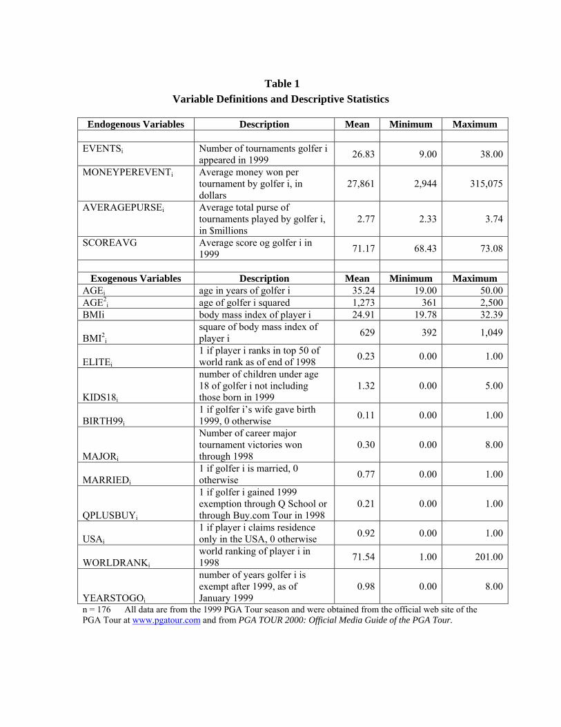
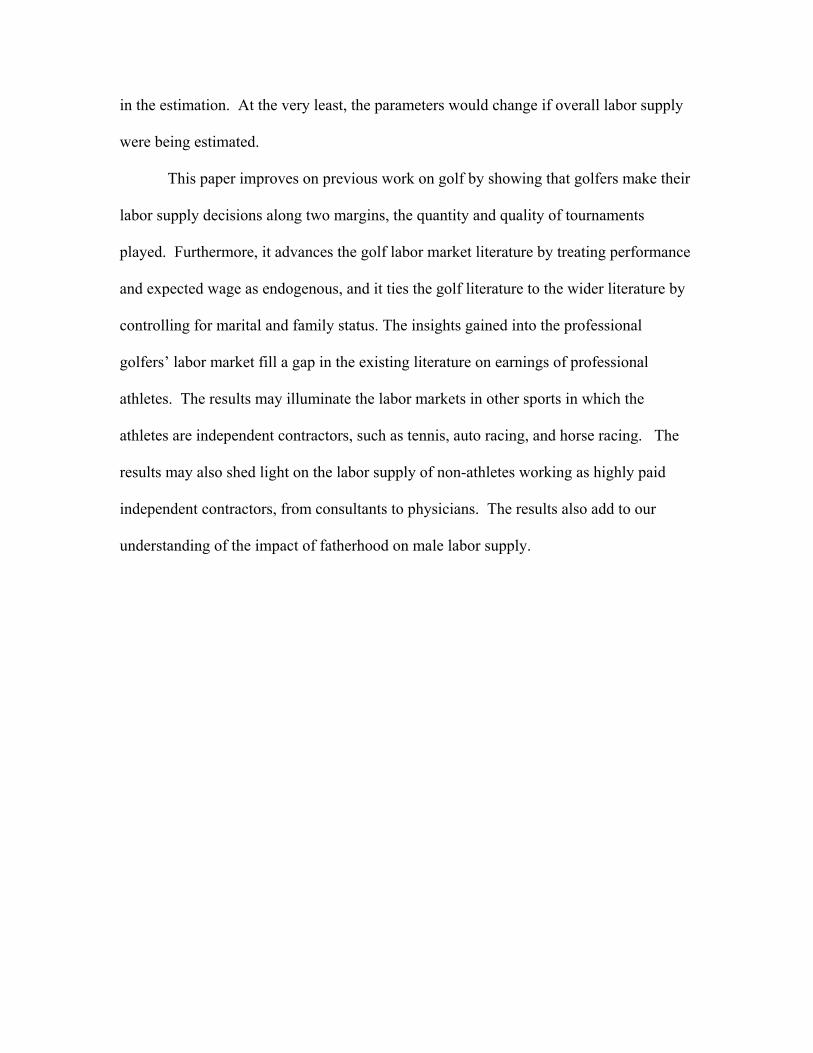
Table 1

Variable Definitions and Descriptive Statistics

Endogenous Variables Description Mean Minimum Maximum

EVENTSi Number of tournaments golfer i appeared in 1999

26.83 9.00 38.00

MONEYPEREVENTi Average money won per tournament by golfer i, in dollars

27,861 2,944 315,075

AVERAGEPURSEi Average total purse of tournaments played by golfer i, in $millions

2.77 2.33 3.74

SCOREAVG Average score og golfer i in 1999

71.17 68.43 73.08

Exogenous Variables Description Mean Minimum Maximum

AGEi age in years of golfer i 35.24 19.00 50.00 AGE2

i age of golfer i squared 1,273 361 2,500 BMIi body mass index of player i 24.91 19.78 32.39

BMI2i

square of body mass index of player i

629 392 1,049

ELITEi

1 if player i ranks in top 50 of world rank as of end of 1998

0.23 0.00 1.00

KIDS18i

number of children under age 18 of golfer i not including those born in 1999

1.32 0.00 5.00

BIRTH99i 1 if golfer i’s wife gave birth 1999, 0 otherwise

0.11 0.00 1.00

MAJORi

Number of career major tournament victories won through 1998

0.30 0.00 8.00

MARRIEDi 1 if golfer i is married, 0 otherwise

0.77 0.00 1.00

QPLUSBUYi

1 if golfer i gained 1999 exemption through Q School or through Buy.com Tour in 1998

0.21 0.00 1.00

USAi 1 if player i claims residence only in the USA, 0 otherwise

0.92 0.00 1.00

WORLDRANKi world ranking of player i in 1998

71.54 1.00 201.00

YEARSTOGOi

number of years golfer i is exempt after 1999, as of January 1999

0.98 0.00 8.00

n = 176 All data are from the 1999 PGA Tour season and were obtained from the official web site of the PGA Tour at www.pgatour.com and from PGA TOUR 2000: Official Media Guide of the PGA Tour.

TABLE 2 Golfer Labor Supply Estimation, lnEVENTS

(two-stage least squares)

Variable Coefficient Estimate t-score AGEi 0.123* (5.00) AGE2

i -0.002* (5.24) BIRTH99i -0.112* (2.42) KIDS18i -0.021 (1.30) MARRIEDi 0.031 (0.76) USAi 0.164* (3.28) YEARSTOGOi -0.011 (1.30) lnMONEYPEREVENTi -0.088* (3.11) QPLUSBUYi -0.034 (0.84) MAJORi -0.061 (3.11) CONSTANT 2.033* (3.75) N = 176 Rsq = 0.4893 *significant at 0.05 level, +significant at 0.10 level

TABLE 3 Golfer Expected Wage Estimation, lnMONEYPEREVENT

(two-stage least squares)

Variable Coefficient Estimate t-score lnSCOREAVG  ‐54.21*  (5.48) 

lnAVERAGEPURSEi  3.759*  (3.14) 

lnEVENTSi 0.280  (0.77) 

AGEi  ‐0.0119*  (2.02) 

CONSTANT  236.71*  (5.39) 

N = 176 Rsq = 0.8176 *significant at 0.05 level, +significant at 0.10 level

TABLE 4

Golfer Expected Performance Estimation, lnSCOREAVG (two-stage least squares)

Variable Coefficient Estimate t-score

lnEVENTSi -0.020* (3.24) RANK98i 0.000* (2.68) lnAVERAGEPURSEi -0.063* (2.96) AGEi 0.000+ (1.79) BMIi 0.010* (2.72) BMI2i -0.000* (2.59) CONSTANT 4.244* (76.75) N = 176 Rsq = 0.5594 *significant at 0.05 level, +significant at 0.10 level

TABLE 5

Golfer Event Quality Estimation, lnAVERAGEPURSE (two-stage least squares)

Variable Coefficient Estimate t-score YEARSTOGOi 0.004+ (1.88) lnSCOREAVGi -3.114* (4.19) lnEVENTSi -0.180* (6.81) QPLUSBUYi -0.038* (4.55) ELITEi 0.073* (5.82) CONSTANT 14.870* (4.67) N = 176 Rsq = 0.8246 *significant at 0.05 level, +significant at 0.10 level