Labor Market Returns to Student Loans · Our thanks to Heidi Berner, Amanda Dawes, Cristian Labra,...

Labor Market Returns to Student Loans

Autores:

Alonso Bucarey

Dante Contreras

Pablo Muñoz

Santiago, Mayo de 2018

SDT 464

Labor Market Returns to Student Loans∗

Alonso Bucarey† Dante Contreras‡ Pablo Munoz§

May 23, 2018

Abstract

This paper studies the labor market returns to a state guaranteed loan (SGL) used to

finance university degrees. Using administrative data from Chile and a regression discontinu-

ity design, we show that nine years after high school graduation students who enrolled at a

university thanks to the SGL attended it for 5 years, foregoing 3 years of vocational education

and accumulating additional 14 thousand dollars in student debt. Strikingly, these students

do not benefit in terms wages, employment, type of contract, or type of employer. The low

quality of institutions attended by loan users may account for these results.

∗Our thanks to Heidi Berner, Amanda Dawes, Cristian Labra, Isidora Palma, Javiera Troncoso, and the Min-isterio de Desarrollo Social of Chile for their help accessing the data. The views expressed here are those of theauthors and do not reflect the views of the Ministerio de Desarrollo Social. We also thank Nikhil Agarwal, DaronAcemoglu, Joshua Angrist, David Card, Seth Zimmerman, Parag Pathak, and MIT Labor field lunch for theiruseful suggestions. Carlos Guastavino provided excellent research assistance. Alonso Bucarey thanks the financialsupport of the National Academy of Education/Spencer Dissertation Fellowship and the George P. and Obie B.Shultz Fund. Dante Contreras acknowledges the financial support provided by the Centre for Social Conflict andCohesion Studies (CONICYT/FONDAP/15130009).†MIT, Department of Economics. Email: [email protected]‡Universidad de Chile, Department of Economics. Email: [email protected]§UC Berkeley, Department of Economics. Email: [email protected]

1 Introduction

In the last decade, several countries have seen a heated debate over the benefits and negative

consequences of student loans. The high labor market returns for higher education together with

the inability to borrow against future returns from education have encouraged the introduction

of different student loan programs intended to democratize access to higher education. However

the idea that student loans may impose a heavy burden on students and their families has raised.

Indeed, the debate over a potential student debt crisis has motivated calls for a redesign of the

student loan system in both developed and developing countries. Unfortunately, most of this

discussion has focused only on anecdotal and correlational evidence.

This paper contributes to the debate by providing causal evidence of the labor market return to

a state guaranteed loan (SGL) for students who enroll at a university thanks to it. We study this

issue in Chile, where a SGL was introduced in 2006 setting sharp eligibility criteria. Chile is an

appealing case for study. First, students gain access to the SGL to finance a university degree

by applying for financial aid and scoring above a fixed cutoff in the centralized college admissions

exam. This institutional feature allow use to implement a fuzzy regression discontinuity design

that exploits the quasi-randomness of loan eligibility as an instrument for its use at a university.

Second, linked administrative data allows to follow students up to nine years after high school

graduation, making it possible to estimate the causal effect of the use of this university loan on

both educational and labor market outcomes.

We find that treated students induced to use a university loan due to their initial eligibility increase

their total years of schooling by two, substituting vocational programs for university degrees.

However, eight years after high school, only 40% of university loan takers have graduated versus

a 65% of ineligible compliers. By year nine out of high school, we find that users of a university

loan have increased their debt by 14 thousand dollars and have experienced a decrease in their

labor market experience of around 1.2 years. Furthermore, we estimate statistically insignificant

effects on wages and employment and we do not find any difference between treated and untreated

students in their type of contract, public sector participation or on the average wage paid by

their employers. We provide suggestive evidence that the low quality of the higher education

institutions chosen by university loan users, measured by years of accreditation and graduation

rate, contribute to explain their null labor market gains. Regression discontinuity-based estimates

show that the university loan induced students to substitute away mostly from top tier vocational

institutions into medium tier universities that have on average one fewer year of accreditation

and a twenty percentage points lower graduation rate. In line with this finding, a model that

interacts institutional characteristics with our quasi-experimental variation shows that proxies of

institutional quality are important determinants of labor market returns.

1

Our focus is on the causal effect of ever using an SGL to attend a university, and our empirical

strategy is a fuzzy regression discontinuity design. This strategy uses the sharp university loan

eligibility cutoff based on the national college admissions test (Prueba de Seleccion Universitaria,

PSU hereafter) and accounts for the voluntary take-up of the loan and students’ ability to retake

the PSU and qualify for the university loan over the years. We implement this strategy with

an instrumental variables approach that uses students’ eligibility status for a university loan on

their first attempt taking the test as an instrument for ever using it. Our first stage estimates

show that being initially eligible increases take-up by 8 percentage points, a 26% increase relative

to the initially ineligible group (with an F-test above 100). Because of the local nature of this

quasi-experiment, our estimates are better interpreted as a local average treatment effect (LATE)

for compliers (Imbens and Angrist, 1994), or those who without initial access to a loan do not

ever enroll at a university using an SGL. We show that compliers to this instrument are poorer

than other students, coming disproportionately from the poorest 20% of the population; they

also have less-educated parents and rely more heavily on public health insurance. Additionally,

compliers have limited alternatives for financing a university degree as none of them are eligible

for scholarships.

This paper makes two main contributions. First, we add to a growing literature on the effects of

financial aid on educational outcomes (e.g. Abraham and Clark, 2006; Angrist et al., 2014; Avery

et al., 2006; Bound and Turner, 2002; Cornwell et al., 2006; Dynarski, 2000; Goodman, 2008;

Kane, 2007; Marx and Turner, 2018).1 In our context, more than 95% of students who took the

PSU and applied for financial aid enrolled in some type of higher education by year nine out of

high school. Thus, the use of a university loan increasing the years of higher education by just

two; motivating students to substitute 3 years of vocational education for 5 years at a university.

Despite this educational upgrade, we find that eligible compliers have a 25 percentage points lower

graduation rate and attend 30% more institutions. Furthermore, 30% of eligible compliers and

17% of ineligible compliers enroll at both university and vocational institution at some point.2

Together, these results suggest that the large short-run effects of loan eligibility on university

enrollment, previously reported by Solis (2017), may have dissipated over time.

Second, we contribute with direct quasi-experimental evidence to an incipient literature on the

effects of student loans on early labor market outcomes (e.g. Rothstein and Rouse, 2011; Rau et

al., 2013; Ji, 2018, Weidner, 2016; Montoya et al., 2017). For this analysis, we use administrative

data from the Unemployment Insurance that covers all formal dependent labor in the private

sector from 2007 to 2017,3 and we provide robustness to our findings by using Pension System

data that include dependent and independent labor in both the public and private sector, but

1Deming and Dynarski (2009) survey this literature.2By year nine out of high school, the percentage of compliers enrolled at a university is very close to zero.

Therefore, our graduation results are not driven by students enrolling for longer periods.3Other work using similar data include Rau et al. (2013), who also study the role of the SGL but implement

2

which we can access for a shorter period of time (2013 to 2015). We show that nine years after

high school graduation, eligible compliers did not experience any statistically significant gain in

wages or their probability of employment. Additionally, we show that the university SGL had no

effect on job security measured by the use of fixed term contracts, on the probability of working

in the public sector, or working for better paying firms. However, we report that university loan

takers experience a decrease of 1.2 years of labor market experience. Finally, administrative data

on SGL borrowers shows that the take-up of a university loan increase debt by 14 thousand dollars.

We interpret the previous results in the light of recent evidence on the heterogeneous labor market

returns to different higher education alternatives (e.g. Hastings et al., 2013; Rodriguez et al., 2016;

Ref para EEUU). We find that compliers attend second- and third-tier universities when eligible

for a university loan and high quality vocational institutions otherwise. These universities have 25

percentage points lower graduation rate and one fewer year of institutional accreditation compared

to the fallback vocational institutions.4 Moreover, using a 2SLS model that separately interacts the

use of university loan with the graduation rate and years of accreditation of the institutions students

attend, we show that on average: i) one standard deviation increase in the graduation rate of the

higher education institutions raises the wages of eligible compliers by 538 dollars (0.58 standard

deviations), and ii) one standard deviation increase of the years of accreditation implies gains of

357 dollars (0.39 standard deviations) for eligible compliers. These findings suggest that the low

return of the loan policy may come from the low quality of the institutions where eligible compliers

are admitted, a result related to that of Cohodes and Goodman (2014) who, in a different context,

show that financial aid could incentivize students to attend institutions with lower graduation

rates.

The rest of this paper is organized as follows. Section 2 discusses some of the institutional features

of the SGL program we study. Section 3 presents the data used in this paper while section 4

explains the empirical strategy. Section 5 shows the main results and section 6 offers a discussion

focused on the role of institutional quality. Finally, section 7 concludes.

2 Background: The State Guaranteed Loan Program

High school graduates applying for admission at 4-year degrees take a college admission score

(Prueba de Seleccion Universitaria, PSU), which includes a Math, Language, Science and His-

a structural approach in a shorter time horizon, and Montoya et al. (2017), who studies the return to universitydegrees vis a vis vocational degrees using ever eligibility for a university loan as instrument. While Rau et al. (2013)and Montoya et al. (2017) report similar reduced form effects to what we find, our study focuses on loan take-up,looking at a larger set of outcomes and providing direct evidence of the importance of the quality of institutionswhere loan takers enroll.

4We classify universities into four tiers according to their selectivity, following Beyer et al. (2015).

3

tory. Scores on each section are normalized within a range from 100 and 850, with mean 500 and

standard deviation of 110. In 2006, the Chilean government introduced a State Guaranteed Loan

program (SGL, hereafter). This policy provides access to loans at any accredited institution to

students who fill out a socio-economic information form (Formulario Unico de Acreditacion So-

cioeconomica, FUAS hereafter) and score above 475 points on the average Math and Language

college admission exam. Students with a high school GPA above 5.27 (GPA ranges 1 to 7) who

pursue 2-year degrees are also granted access to a loan. Figure 1 shows that the data conforms to

these sharp eligibility requirements. Panel A shows the total first-year student debt at any type of

institution, and Panel B restricts to debt at universities. This form helps the government deter-

mine family income quintiles. Although the SGL program was initially meant to benefit students

in the first four income quintiles, conversations with individuals involved in the implementation

of the loan program and our own analysis of the data shows that individuals in the fifth income

quintile also became eligible in years when there was enough funding.

Applicants to the loan know about their eligibility status before enrolling in higher education, and

the general terms of the loan are publicly available. Because SGL eligibility cutoffs were established

in 2006 and have remained the same since then, students considering higher education alternatives

can easily learn their eligibility status for an SGL at different types of institutions after their PSU

tests are graded. Moreover, the government and higher education institutions advertise students

eligibility to receive the guaranteed loan. Some institutions and degrees are allowed to impose

different requirements for loan eligibility, above those established by the Law. These institution

specific requirements are also available to students at the time of enrollment. During the years of

our study, the conditions of the loan were a 6% real interest rate; a fixed payment over a period of

5, 10, or 15 years, depending on the total debt; and a grace period of 18 months before students

have to make the first payment following their graduation or drop out date. Additionally, condi-

tional on being in good academic standing, students could finance their degree for up to 3 years in

excess of the official duration in the case of university degrees and for 2 years for vocational degrees.

Students can use the SGL at any accredited institution. Accreditation is responsibility of an in-

dependent agency (Comision Nacional de Educacion, CNA) which decides whether an institution

receives accreditation or not (and by how many years) based on different records from the uni-

versity and external auditors. Since the introduction of the SGL, the total number of accredited

institutions has increased. Table A.1 in the appendix shows that the number of accredited univer-

sities raised from 14 in 2004 to 45 in 2016. As of today, 64.3% of all higher education institutions

are accredited. However, there is significant heterogeneity in the number of years for which they

receive the accreditation, and degrees might not be accredited even when the institution receives

accreditation.

4

After enrolling at the accredited institution of their choice, students can borrow up to a degree-

institution specific maximum. The degree-institution cap for borrowers is on average 90% of the

tuition, and students, their families, or scholarships would have to cover the difference. Alternative

financing options include another university loan available only for students enrolled at a CRUCH

university5 and government-provided scholarships. For the cohorts in our analysis, students among

the poorest 40% who scored above an average of 550 points on the Mathematics and Language

exams of the PSU have access to scholarships that partially covered tuition at 4-year degrees,

while students with a GPA above 5.0 are eligible for scholarships at 2-year degrees. However, most

students who did not meet the minimum eligibility requirement for a loan would probably have

trouble funding their education with a private loan. According to the nationally representative

household survey CASEN, only 7.5% of the loans held by all students in 2015 came from private

banks (without State guarantee).

Since its implementation, the total debt held by students has increased at a rate of 70% per year,

and the total number of students holding a student loan increased from 15.8 thousand students in

the first year of operation to 652 thousand students by 2016. Figure 2 presents the evolution of

both the number of students using the SGL and the total debt that they hold. As these figures

increased, commentators started arguing about the heavy burden that student debt imposes on

borrowers and debating whether the rising outstanding debt should be of public concern. In fact,

in April 2018 congress created a commission to reformulate the SGL and investigate whether debt

negatively affected students. The Chilean government is currently considering a complete reform

of the SGL.

3 Data and Descriptive Statistics

The Chilean government provided the data, which include demographic information, test scores,

enrollment, graduation, financial aid, and labor market outcomes from 2007 to 2017. Our analysis

sample consists of students who graduated from high school in 2007 or 2008, took the college

admission test immediately, and filled their socio-economic information to access financial aid. For

these students we observe enrollment in higher education, their loan take-up, their graduation, the

characteristics of their degrees, as well as their labor market participation, wages, and employers’

characteristics up to nine years after high school graduation.

5The Traditional University Loan program, called Fondo Solidario de Credito Universitario, covers only CRUCHstudents scoring above 475 points.

5

Labor market outcomes come from the the Unemployment Insurance (UI) system, which covers all

dependent labor in the private sector between January 2007 and October 2017, and the Pension

System (PS) dataset, which we access from 2013 to 2015 and includes dependent labor in both

the public and private sector and approximately 14% of all independent labor who voluntarely

contribute to the pension system. We conduct most of our analysis using UI data, and use the PS

dataset to study public sector work and to check the robustness of our results to the inclusion of

independent labor that contribute to the pension system.

Financial aid applicants and students in our RD sample are poorer than the general population of

test takers. Table 1 reports descriptive statistics for test takers, financial aid applicants, students

eligible for a university loan, and students within a bandwidth of 40-points around the cutoff (RD

sample).6 Column (2) shows that financial aid applicants are more likely to have attended a public

high school, have public health insurance as opposed to private, and have less-educated parents.

In contrast, column (3) shows that students who qualify for a university loan, scoring above 475

points, come from a higher socioeconomic background. Our RD sample, in column (4), has similar

characteristics to the rest of financial aid applicants. No student in this sample is eligible for

a state-provided scholarship, a byproduct of the test score window of this sample that excludes

scholarship-eligible students. Finally, we also see that the labor market outcomes of students in

these four samples are similar.

Institutions of different selectivity level differ markedly. Table 2 presents a comparison of univer-

sities and vocational institutions at different selectivity tiers. University tiers were constructed

following Beyer et al. (2015) so that lower-tier institutions have higher average Math and Lan-

guage admission scores and a higher share of students taking the admission test. Top vocational

institutions have a share of students who took the college admission test above the median. Ta-

ble 2 shows large heterogeneity in terms of institutional characteristics. Compared to the rest of

institutions, more selective universities and top vocational institutions have more students with a

scholarship, a higher share of accredited degrees, more years of accreditation, a higher graduation

rate, and a higher tuition. For our analysis, we focus on middle-tier universities and top vocational

institutions which concentrate most of the students using the SGL.

On the one hand, second-tier universities are better than or similar to top vocational institutions

in terms of years of accreditation, graduation rate, and the share of students with scholarship. On

the other hand, third-tier universities are worse than top vocational institutions along all these

dimensions. It is also worth noting that vocational institutions are significantly cheaper and less

selective than second- and third-tier universities. Finally, the two types of institutions that concen-

6These 40-points correspond to 0.36 standard deviations of the running variable.

6

trate the smallest share of students with an SGL (first- and fourth-tier universities) are at opposite

extremes in terms of their characteristics and they enroll fewer students using SGL for opposite

reasons. Students enrolled at first-tier universities have more access to merit-based scholarships,

decreasing their need for loans. Meanwhile, 18% of universities in the fourth-tier are not accred-

ited, which makes their students ineligible to use the SGL.

4 Empirical Framework

The primary relation of interest is

Yi = βLi + f(ri, Zi) + ei (1)

where Y are educational and labor market outcomes for student i in year t; Li is an indicator of

treatment equal to one if the student ever used an SGL to enroll at a university; f(ri, Zi) is a

function of the running variable ri = (Average Math and Languagei − 475) where the Math and

Language correspond to the score in the first attempt at the college admission exam; and the ini-

tial eligibility dummy, Zi = 1(ri > 0), equals 1 if the scored above 475 in the first attempt at the

college admission exam. Our definition of treatment captures enrollment at a university using the

SGL. Thus, untreated students are either those who enroll at a university without an SGL, those

who attend vocational institutions, or those who do not enroll at any higher education program.

An obvious threat to identification in this setting is that the decision of taking up a SGL to attend

a university may be related to potential earnings and comparative advantage, so an ordinary least

squares (OLS) estimation of equation (1) may not recover causal the effects of loan use. Therefore,

we use a fuzzy regression-discontinuity design to estimate university loan effects. Specifically, we

exploit the quasi-random eligibility for university loans induced by the test score cutoff described

in section 2. To implement this, we estimate equation (1) by two-stage least squares (2SLS), with

first-stage equation

Li = πZi + g(ri, Zi) + vi (2)

where g(ri, Zi) is a function of the running variable ri and the university-loan initial eligibility indi-

cator Zi. In our setting, where students cannot manipulate the exact score they get, the first-stage

7

exploits the quasi-random nature of initial eligibility around the eligibility cutoff. For estimation,

we specify f(ri, Zi) and g(ri, Zi) as a linear function of ri with a change of slope at each side of

the cutoff. Figure 3 plots the university loan take-up among students who initially applied for

financial aid and those who did not, confirming the importance of initial eligibility on ever taking

up the university loan. Plotted points are conditional means for all students in our analysis sample

within a two-points binwidth of the average Math and Language scores obtained by the students

at their first PSU attempt. Panel A shows the increase in university loan take-up among students

who cross the first-year eligibility cutoff. As previously reported by Solis (2017), immediately after

high school graduation, university loan take-up jumps from 0 to 15% for students who applied for

financial aid and scored above 475 points. On the other hand, students who did not apply for

financial aid in their first attempt have no access to the SGL. The figure also shows that above

550 points, loan take-up starts decreasing due to the increase in scholarship availability at higher

test score levels.

Panel B of Figure 3 graphically shows the first stage of our design. Crossing the initial eligibility

cutoff increases discontinuously the probability of ever taking up a university loan. In this panel,

we see that even students who initially did not cross the cutoff or did not apply for financial aid can

access the SGL at some point in the future, highlighting the fuzzy nature of this quasi-experiment.

Even without being initially eligible, students have the ability to retake the college admission test

or get an SGL as second-year students at their universities. Nonetheless, initial eligibility around

the cutoff is an important determinant of its use.

Estimates of equation (2) show that initial eligibility for the university loan, which is deterministic

and sharp, significantly increases loan take-up, which remains probabilistic over time. Within a

bandwidth of 40 points, initial eligibility increases the probability of ever taking up a university

loan by 8 percentage points, a 35% increase with respect to the 23% take-up among initially in-

eligible students. This effect is precisely estimated with a standard error of 0.008, which implies

a strong first-stage with an F-test above 100. Moreover, our design passes the standard test of

non-manipulation of the running variable and it exhibits balanced covariates between treated and

untreated students.7

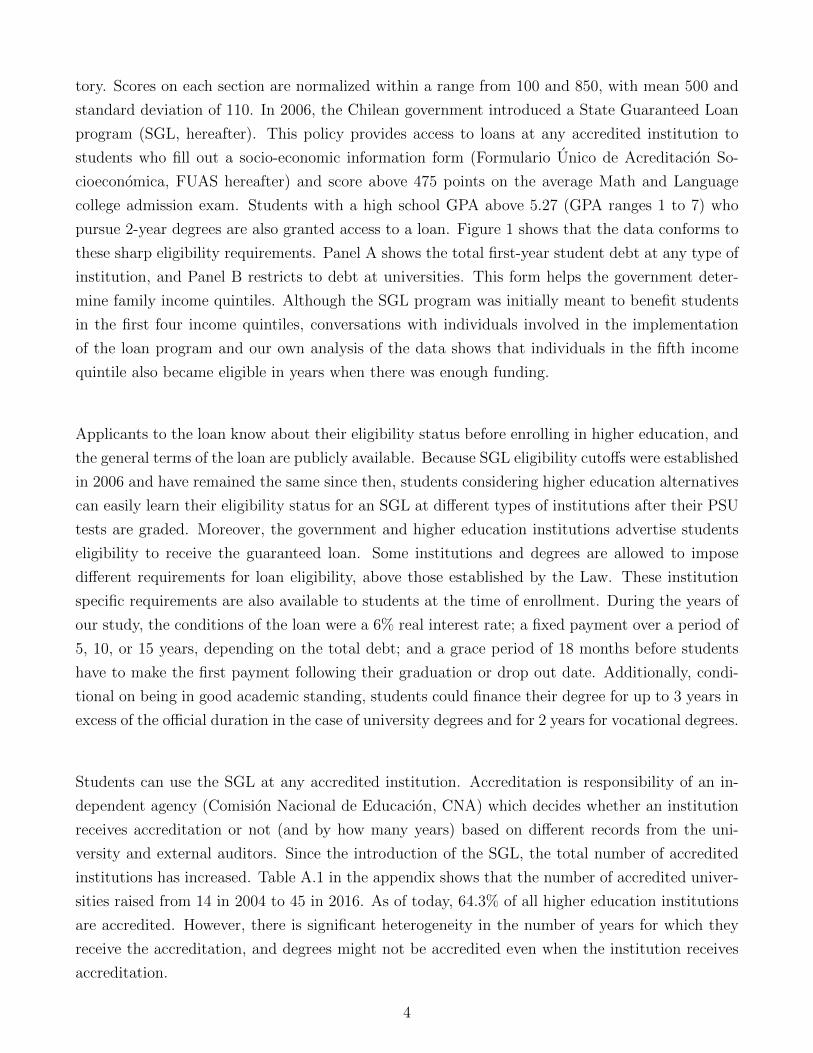
Visual inspection of the density of the running variable in Figure 4 and overlapping confidence

intervals of density estimates at both sides of the cutoff indicate no manipulation on the centrally

administered tests used to construct the running variable. Reassuringly, the tests proposed by

7We report results using outcome specific bandwidths selected using the robust criteria in Calonico et al. (2014)in tables A.2 to A.5.

8

Cattaneo et al. (2016, 2017) and McCrary (2008) fail to reject the null hypothesis of equal densi-

ties around the cutoff. Students who scored above the cutoff look much like students who scored

below it. Table 3 presents a simple comparison of baseline characteristics for students at both

sides of the cutoff. These calculations include all students in our analysis sample within a 40-

points binwidth of the eligibility cutoff. Column (1) displays the mean characteristics for students

who are below the cutoff, while column (2) reports the estimated difference by eligibility status

around the cutoff. These coefficients come from regressions of each baseline characteristic on the

initial eligibility indicator Zi, substituting Li by the corresponding characteristic in equation (2).

Mean differences are small as reflected by the 95% confidence intervals in columns (3) and (4)

and we do not find any economically or statistically significant difference among students at both

sides of the cutoff, indicating that random assignment around the cutoff is a reasonable assumption.

In our context, standard LATE assumptions imply that initial university loan eligibility only in-

fluences labor market outcomes through the use of the loan to enroll at university, and that initial

loan eligibility weakly increases the take-up for all students. Under these assumptions, the 2SLS

estimate of β in equation (1) may be interpreted as a local average treatment effect (LATE). This

is an average causal effect of the SGL use for compliers, those students who use the loan at some

point to enroll at a university only if they are initially eligible, and who without being initially eligi-

ble will never use the loan to enroll at a university (Imbens and Angrist, 1994; Angrist et al., 1996).

In our setting, compliers are likely to be in need of financial aid to access university. Table 4

presents the average demographic characteristics for the whole analysis sample and for eligible

compliers whose average characteristics are estimated following Abadie (2002). Panel A shows

that eligible compliers, in column (3), are more likely to have parents who did not pursue higher

education, are more likely to have public health insurance as opposed to private insurance, and did

not attend private high schools. Additionally, Panel B shows that 51% of university loan-eligible

compliers come from families among the poorest 20% in the country, compared to 36% for the

entire university loan-eligible population. Finally, Panel C shows that take-up of the university

loan among the eligible population is 36%, and that nobody in the complier population gained

access to a university scholarship.

9

5 Results

5.1 Effects of the University Loan on Education

Initial eligibility for the university loan did not have an effect on the decision of ever enrolling

in some form of higher education; it did, however, encourage students to substitute vocational

education in favor of university degrees and increase the total years of schooling. Figure 5 plots

conditional means of an indicator for ever enrolling in higher education up to nine years after

graduation from high school as a function of the running variable, and it also shows estimated

conditional mean functions smoothed using local linear regression. Panel A shows that students

above and below the cutoff enrolled in some form of higher education at least once throughout

the nine years post high school graduation, with students above the cutoff substituting vocational

education for university degrees, as shown in panels B and C. Despite the null extensive margin

effect, Figure 6 shows that initial eligibility increased the overall years of higher education. Panel

A shows reduced form evidence that students who are initially eligible for the loan increase their

overall education in 0.18 years, with students increasing university attainment in 0.43 years and

reducing attainment at vocational degrees in 0.25 years as shown in panel B and C.

Table 5 summarizes the previous reduced form effects and presents 2SLS estimates. The first row

in this table presents the first stage, with initial university loan eligibility boosting the probability

of ever taking up a university student loan by 8 percentage points over a mean take-up below the

cutoff of 23 percentage points (35% effect). Column (1) shows the reduced form differences in

enrollment between initially eligible students and students who, by a small margin, did not cross

the cutoff. These estimates summarize the magnitudes displayed in Figures 5 and 6.

Column (3) in Table 5 presents the 2SLS coefficients, which in our just identified IV model cor-

respond to the reduced form effects scaled by the first stage coefficient. We find that taking up a

university loan increases the probability of ever enrolling at a university by 83 percentage points,

while decreasing ever enrollment at a vocational degree by 71 percentage points. We also find that

taking up the university loan increases the total years of higher education by 2.1, similar to the

difference in nominal duration between a university degree and a vocational degree. In fact, those

who are induced by initial eligibility to take up the university SGL gain 5.1 years in university while

giving up 3 years in vocational institutions. An important caveat when interpreting this last result

is that the take-up of the university SGL increases the number of institutions in which students

pursue a degree by 30%. Moreover, Table 5 shows that taking the loan at a university decreases

graduation by 25 percentage points by year eight out of high school. This suggests that the loan

10

helped students move from a vocational degree into a university but decreased their chances to

finish any degree.

Column (2) presents the complier mean among untreated students, E[Yi(0)|Li1 > Li0] in the po-

tential outcomes notation. These are computed following Abadie (2002).8 These estimates show

that all ineligible compliers attended vocational education, and 17 percentage of them attended

both types of education. This implies that 30 percent of all eligible compliers attended both types

of education. 9 Column (4) shows the corresponding OLS estimates in our RD sample. OLS

estimates generally underestimate the impact of loan take-up on schooling, suggesting significant

selection into loan take-up.

These results are not significantly affected by students being enrolled in higher education at the

time of our measurement. Figures 7 to 9 plot initially eligible and ineligible complier means of

the educational outcomes for each year after high school. These figures show that nine years after

high school, the total number of years of schooling and the enrollment status converged between

eligible and ineligible compliers. Panel A of Figure 7 presents the fraction of students enrolled at

a university between 1 and 9 years after high school, with panel B displaying analog results for

vocational degree enrollment. Enrollment rates at both types of institutions decline significantly

over the years, and there is convergence between treated and untreated compliers by year 9 out

of high school. Moreover, by the end of our sample window, enrollment is less than 10% in both

vocational and university institutions. Analogously, Figure 8 shows that 7 years after high school

graduation the years of schooling at each type of institution convergence. Additionally, Figure 9

shows that the proportion of students holding a degree increases over the years to reach a 40%

among the treated compliers and 65% among untreated compliers. Although the graduation rate

from university degrees does not show convergence, the fact that the average number of years is

stable and that the enrollment rate declines to zero indicates that a significant graduation increase

is unlikely.

5.2 Effects of the University Loan on Debt and Labor Market Out-

comes

Students who score above the initial eligibility cutoff have higher debt and similar earnings com-

pared to students who were ineligible by a small margin. Figure 10 shows reduced form evidence

8We regress (1− Li)Yit = ρ(1− Li) + f(ri, Zi) + vi where ρ is an estimate of E[Yit(0)|Li1 > Li0].9This comes from adding up the 17 percentage points among ineligible compliers and the 12 percentage points

treatment effect in attendance of both types mentioned before.

11

of the increase in total accumulated student debt at any type of institution nine years after high

school graduation. Students just above the cutoff accumulate on average 1.2 thousand dollars

higher debt, an unsurprising result given that they also enroll longer and at institutions that are

more expensive.10 More surprising is that students end up with a similar level of earnings regard-

less of their initial loan eligibility status. Figure 11 shows the average monthly wage of students

nine years after high school, where the difference around the cutoff is just -4.5 dollars. We find

similar reduced form patterns for the probability of being employed, the probability of having a

fixed term contract, the probability of part-time job, and for employers’ characteristics such as

firm size and wage bill.

Turning to the causal estimate of a university SGL on debt and earnings, Table 6 presents again

the first stage results at the top, the reduced form effects in column (1), and 2SLS estimates in

column (3). This last column shows that students who are induced to take up a university student

loan because of their initial eligibility (the compliers) accumulate 14.3 thousand dollars more debt.

In column (2), we see that the mean debt for students who are not initially eligible is 3 thousand

dollars, which is explained by their eligibility for a loan at a vocational institution, their posterior

eligibility to a loan at a university, and by the ability of students to borrow once they enroll as

second-year students in good academic standing.

The estimated causal effect of loan take-up on earnings is not statistically different from zero. Ta-

ble 6 also shows the effect on the probability of employment, without any significant effect. Both

of these results are robust to the inclusion of independent and public sector workers as shown in

Panel C of Table 6. Additionally, students around the cutoff work at firms with similar average

wage, leaving little room for differential career parts arising from firm effects (e.g. Card et al.,

2018). Moreover, and unlike in previous studies (e.g. Rothstein and Rouse, 2011), we do not find

any effect of the treatment on the probability of working in the public sector.11 Finally, the only

significant effect we find on labor market outcomes is a reduction of labor market experience of

1.2 years as a result of university loan take-up. In Appendix B, we follow a mincerian approach to

show that the negative wage effect that arises from the decrease in experience could only account

by the null effect of the SGL on wages if the returns to initial loan take-up at university are low

enough compared to enrolling at a vocational institution. In the next section, we show that the

low quality of the receiving institutions of compliers helps to explain why the average labor market

return to university vis a vis vocational is low.

10The reduced form effect of initial university loan eligibility on the cost of the tuition of the first degree is 100dollars.

11This setting is different from Rothstein and Rouse (2011) in the sense that they evaluate the effect of taking ornot taking up a loan, while we study the effect of taking up a loan for university in a context where the counterfactualfor treated compliers includes the possibility of using loans for vocational studies.

12

6 Discussion

Given the switch in enrollment towards universities and the increase in the number of years of

higher education, the null effect of the university SGL on labor market outcomes might be surpris-

ing. In this section, we explore to what extent the quality of destination institutions of compliers

can account for this result. In the spirit of Abdulkadiroglu et al. (2014) and Abdulkadiroglu et

al. (2018), we start by characterizing the educational fallbacks for untreated compliers and the

destination of treated compliers. Then, we evaluate treatment effect heterogeneity by exploiting

variation in the characteristics of the universities at which compliers enrolled.

6.1 Destination of Compliers

The destination of treated compliers and the fallback of untreated compliers are important to

understand the RD-based estimates presented before. For instance, if students without initial

access to the loan attend schools with similar or better performance than the institutions in which

loan takers enroll, then the zero labor market effect might emerge naturally as a consequence of the

high returns in fallback schools rather than as a consequence of low performance of the universities

that treated compliers attend. To explore this hypothesis, we characterize the mix of schools that

define the loan complier destinations and fallbacks. Specifically, we implement Abadie (2002)’s

methods to estimate the the ineligible compliers fallback options with the equation:

Cs(i)(1− Li) = (1− Li)γ + ari + criLi + εi (3)

instrumenting (1−Li) with the initial eligibility indicator Zi. Here, s(i) indicates the first institu-

tion attended by student i, and Cs(i) is the characteristic of that institution. The 2SLS coefficient

γ captures the average of the institution characteristic Cs(i) for untreated compliers. Similarly,

we can replace (1 − Li) by Li at both sides of the equation estimate the mean characteristics of

destination institutions of treated compliers.

Table 7 presents the fallbacks and destinations of compliers to the initial eligibility instrument

for the SGL. Columns (1) and (2) show mean characteristics for students eligible and ineligible

13

to take-up a university loan, columns (3) and (4) report eligible and ineligible complier means

coming from 2SLS estimates of equation (3), and column (5) reports treatment effects. Column

(5) of Panel A shows that loan take-up increases the years of enrollment at second- and third-tier

universities, without a meaningfully impact on attendance to first-tier universities. Column (4) of

this panel shows that the main fallback for the untreated compliers are top vocational institutions.

Indeed, years of enrollment at top vocational institutions decreased by almost 3 years as a con-

sequence of loan take-up. Therefore, the main effect of the loan program was to divert students

from high quality vocational programs into low- to medium-quality universities.

Panel B in Table 7 reports the years of accreditation and graduation rates of the institutions at

which eligible and ineligible compliers enroll. These results come from estimation of equation (3)

setting C {s(i)} equal to the years of accreditation of institution s(i) and its graduation rate. This

panel shows that compliers move to institutions with one fewer year of accreditation and with 25

percentage points lower graduation rate. These findings, together with recent research showing

that the labor market returns of different higher education alternatives can be heterogeneous in

Chile (Hastings et al., 2013; Rodriguez et al., 2016), suggest that the zero effect of university

loan take-up could be related to the better quality of fallback vocational institutions relative to

destination universities.

6.2 The Role of Institutional Quality

The characteristics of fallback and destination institutions presented in Table 7, together with the

descriptive statistics in Table 2 suggest that the university loan pushed students to enroll at worse

institutions. To investigate whether these characteristics can explain the null labor market effect

of the university loan, Table 8 reports relationships between loan take-up and institutional quality

measured by years of accreditation and graduation. The results from this section come from a

just-identified model and rely on a constant effects assumption. Specifically, we extend the 2SLS

model presented before to include an interaction between loan take-up and characteristics of the

institutions,

Yi = β0Li + β1Li(Xi − X) + f(ri, Zi) + ei (4)

where (Xi − X) is the demeaned characteristic of the institution attended by student i. In this

case, we use the interaction between initial eligibility and the corresponding demeaned institutional

characteristic as an additional instrument for Li and Li(Xi − X). The first stage F-test on these

14

interacted models is above 90.

Columns (1) and (2) of Table 8 show estimates from 2SLS models interacting loan take-up with

the demeaned number of years of accreditation of the attended institution. The interaction coef-

ficients for years of accreditation show that institutions with above average years of accreditation

are more expensive and drive higher levels of debt, but they also improve labor market outcomes.

An increase in one standard deviation in the years of accreditation (1.6 years) increases wages by

357 dollars, the probability of employment by 18 percentage points, and the average wage of the

firm by 588 dollars. Estimates of these interactions are reasonably precise and imply that treated

compliers’ earnings are being affected by the fewer years of accreditation of some of the institutions

they are induced to attend as a result of the SGL.

Columns (3) and (4) of Table 8 report results from models that interact university loan take-up

with the demeaned graduation rate of the institutions. The estimates of panel A show that in-

stitutions with above average graduation rates lead students to accumulate slightly lower levels

of debt, reduces the number of institutions attended, and increases their chances of graduation.

Consistently, Panel B shows that better graduation rates lowers the probability of part-time or

temporary work, while also providing higher earnings, increasing the probability of employment,

and raising the likelihood of getting a job at a better paying firm. From panel B, we observe that a

one standard deviation increase in graduation rate (0.5) increases wages by 538 dollars, probability

of employment by 21 percentage points, and the average wage paid by the employer by 388 dollars.

Finally, panel C shows the robustness of these interaction effects to the inclusion of independent

workers and interestingly, it also suggests that students attending better institutions have a lower

probability to hold a job in the public sector.

7 Conclusion

We find that the take-up of a university state guaranteed loan induces eligibility-marginal students

to move away from high quality vocational institutions into medium quality universities (as mea-

sured by years of accreditation and graduation rates). Nine years after high school graduation,

students who took-up the university loan hold 14,000 more dollars in debt and have 1.2 fewer years

of labor market experience. However, their wages, employability, job security and firm character-

istics are no different from those of untreated students. Overall, our findings depict a concerning

15

picture for the average student who decided to enroll at a university using the SGL.

We provide suggestive evidence that the quality of higher education institutions has a key role in

determining whether students can complete their degrees and benefit in the labor market. Our

results also highlight the importance of improving postsecondary institutions whose years of ac-

creditation and completion rates are low. Alternatively, our results should call the attention of

policy makers on the need to redefine the set of institutions that are eligible for this loan. Al-

though the estimates presented here are only valid for compliers at the margin of eligibility, we

believe that these results are informative for a relevant group of students who would not have

attended university without a loan. Most of these students come from families at the bottom of

the the income distribution, but despite their socioeconomic background, they decided to take the

college admissions exam and applied for financial aid, a signal of their willingness to pursue higher

education.

Finally, we have shown that most students are out of higher education at the time we measure

their labor market outcomes. However, our paper is silent about longer-run effects of this policy.

Short-run and long-run effects might differ, for instance, if experience profiles were significantly

steeper for university loan takers. Nonetheless, our results speak to the current debate about the

labor market performance of the first generations of students who the SGL intended to help. How

these students fare in the long-run is an important task for future work.

16

References

[1] Abadie, A. (2002): “Bootstrap Tests for Distributional Treatment Effects in Instrumental

Variable Models,” Journal of the American Statistical Association, 97(457), 284–292.

[2] Abdulkadiroglu, A., J. Angrist, and P. Pathak (2014): “The Elite Illusion: Achieve-

ment Effects at Boston and New York Exam Schools,” Econometrica, 82(1), 137–196.

[3] Abdulkadiroglu, A., P. A. Pathak, and C. R. Walters (2018): “Free to Choose:

Can School Choice Reduce Student Achievement?,” American Economic Journal: Applied Eco-

nomics, 10(1), 175–206.

[4] Abraham, K. G., and M. A. Clark (2006): “Financial aid and students’ college decisions

evidence from the District of Columbia Tuition Assistance Grant Program,” Journal of Human

resources, 41(3), 578–610.

[5] Angrist, J., D. Autor, S. Hudson, and A. Pallais (2014): “Leveling Up: Early Results

from a Randomized Evaluation of Post-Secondary Aid,” Working Paper 20800, National Bureau

of Economic Research.

[6] Angrist, J. D., G. W. Imbens, and D. B. Rubin (1996): “Identification of causal effects

using instrumental variables,” Journal of the American statistical Association, 91(434), 444–455.

[7] Avery, C., C. Hoxby, C. Jackson, K. Burek, G. Pope, and M. Raman (2006): “Cost

Should Be No Barrier: An Evaluation of the First Year of Harvard’s Financial Aid Initiative,”

Working Paper 12029, National Bureau of Economic Research.

[8] Beyer, H., J. Hastings, C. Neilson, and S. Zimmerman (2015): “Connecting student

loans to labor market outcomes: Policy lessons from chile,” American Economic Review, 105(5),

508–13.

[9] Bound, J., and S. Turner (2002): “Going to war and going to college: Did World War

II and the GI Bill increase educational attainment for returning veterans?,” Journal of labor

economics, 20(4), 784–815.

[10] Calonico, S., M. D. Cattaneo, and R. Titiunik (2014): “Robust nonparametric con-

fidence intervals for regression-discontinuity designs,” Econometrica, 82(6), 2295–2326.

[11] Card, D., A. R. Cardoso, J. Heining, and P. Kline (2018): “Firms and labor market

inequality: Evidence and some theory,” Journal of Labor Economics, 36(S1), S13–S70.

[12] Cattaneo, M. D., M. Jansson, and X. Ma (2016): “rddensity: Manipulation testing

based on density discontinuity,” The Stata Journal (ii), pp. 1–18.

17

[13] (2017): “Simple Local Polynomial Density Estimators,” Unpublished.

[14] Cohodes, S. R., and J. S. Goodman (2014): “Merit aid, college quality, and college

completion: Massachusetts’ Adams scholarship as an in-kind subsidy,” American Economic

Journal: Applied Economics, 6(4), 251–85.

[15] Cornwell, C., D. B. Mustard, and D. J. Sridhar (2006): “The enrollment effects

of merit-based financial aid: Evidence from Georgia’s HOPE program,” Journal of Labor Eco-

nomics, 24(4), 761–786.

[16] Deming, D., and S. Dynarski (2009): “Into College, Out of Poverty? Policies to Increase

the Postsecondary Attainment of the Poor,” Working Paper 15387, National Bureau of Economic

Research.

[17] Dynarski, S. (2000): “Hope for Whom? Financial Aid for the Middle Class and Its Impact

on College Attendance,” Working Paper 7756, National Bureau of Economic Research.

[18] Fan, J., and I. Gijbels (1996): Local polynomial modelling and its applications, no. 66 in

Monographs on statistics and applied probability series. Chapman and Hall.

[19] Goodman, J. (2008): “Who merits financial aid?: Massachusetts’ Adams scholarship,” Jour-

nal of public Economics, 92(10-11), 2121–2131.

[20] Hastings, J. S., C. A. Neilson, and S. D. Zimmerman (2013): “Are Some Degrees

Worth More than Others? Evidence from college admission cutoffs in Chile,” Working Paper

19241, National Bureau of Economic Research.

[21] Imbens, G. W., and J. D. Angrist (1994): “Identification and Estimation of Local Average

Treatment Effects,” Econometrica, 62(2), 467–475.

[22] Ji, Y. (2016): “Job Search under Debt: Aggregate Implications of Student Loans,” Unpub-

lished.

[23] Kane, T. J. (2007): “Evaluating the impact of the DC tuition assistance grant program,”

Journal of Human resources, 42(3), 555–582.

[24] Marx, B. M., and L. J. Turner (2018): “Borrowing Trouble? Human Capital Investment

with Opt-In Costs and Implications for the Effectiveness of Grant Aid,” American Economic

Journal: Applied Economics, 10(2), 163–201.

[25] McCrary, J. (2008): “Manipulation of the running variable in the regression discontinuity

design: A density test,” Journal of Econometrics, 142(2), 698 – 714.

18

[26] Montoya, A. M., C. Noton, and A. Solis (2017): “Returns to Higher Education:

Vocational Education vs College,” Documentos de Trabajo 334, Centro de Economia Aplicada.

[27] Rau, T., E. Rojas, and S. Urzua (2013): “Loans for Higher Education: Does the Dream

Come True?,” Working Paper 19138, National Bureau of Economic Research.

[28] Rodrıguez, J., S. Urzua, and L. Reyes (2016): “Heterogeneous Economic Returns to

Post-Secondary Degrees: Evidence from Chile,” Journal of Human Resources, 51(2), 416–460.

[29] Rothstein, J., and C. E. Rouse (2011): “Constrained after college: Student loans and

early-career occupational choices,” Journal of Public Economics, 95(1-2), 149–163.

[30] Solis, A. (2017): “Credit access and college enrollment,” Journal of Political Economy,

125(2), 562–622.

[31] Weidner, J. (2016): “Does Student Debt Reduce Earnings?,” Unpublished.

19

Tables and Figures

Table 1: Descriptive statistics for students

Test takers Analysis sampleUniversity loan

eligibleRD sample

(1) (2) (3) (4)

Female 0.54 0.57 0.53 0.59

Public high school 0.36 0.40 0.34 0.42

Voucher high school 0.52 0.56 0.60 0.57

Private high school 0.11 0.04 0.06 0.01

Average Math and Language college

admission score496.6 509.6 566.3 477.0

High school GPA (from 1 to 7) 5.60 5.70 5.86 5.57

Public health insurance 0.67 0.72 0.67 0.77

Mother with more than high school 0.28 0.25 0.33 0.18

Father with more than high school 0.33 0.30 0.38 0.22

Father monthly wage (dollars) 518.9 474.2 515.9 429.3

Have information on father wage 0.39 0.41 0.42 0.41

Ever taking up a university loan 0.21 0.28 0.36 0.31

University scholarship eligibility 0.09 0.16 0.25 0.00

Observations 298,859 177,470 113,059 53,416

Panel A. Demographics at the time of high school graduation

Panel B. Financial aid

Notes: This table reports descriptive statistics for different samples of high school students. Column (1) considers

students graduating from high school in 2007 and 2008 who took the college admission test (PSU) right after high

school graduation. This corresponds to 72% of all high school graduates. Column (2) further restricts the sample

to students who filled a financial aid application; this is our analysis sample. Column (3) further restricts the

sample to students who scored above 475 points on average on the Mathematics and Language sections of the

PSU. Finally, column (4) includes students in the analysis sample with an average Mathematics and Language

score around the eligibility cutoff in a 40-point bandwidth. Admission scores presented in panel A have a mean of

500 and a standard deviation of 110 points, and GPA ranges between 1 and 7 with a mean of 5.56 and standard

deviation of 0.55.

20

Table 2: Descriptive statistics for higher education institutions

Tier 1 Tier 2 Tier 3 Tier 4 Top Bottom

(1) (2) (3) (4) (5) (6)

Took admission test 0.65 0.52 0.38 0.24 0.31 0.17

Average Math and Language score 640.5 557.6 492.8 452.8 445.3 418.6

Students with a state guaranteed loan 0.07 0.18 0.16 0.02 0.21 0.05

Students with a scholarship 0.28 0.19 0.04 0.01 0.20 0.14

Panel B. Institutional characteristics weighted by first year enrollment in 2008

Number of institutions 10 26 15 8 55 60

Average number of degrees 299.8 127.5 103.6 46.0 76.2 33.2

Total enrollment 29,629 50,279 23,268 4,652 63,290 13,663

Accredited degree 0.49 0.26 0.08 0.06 0.03 0.00

Accredited institution 1.00 1.00 0.97 0.82 0.96 0.62

Years of accreditation 5.98 4.44 2.81 1.74 4.99 1.86

Graduation rate 0.60 0.50 0.40 0.31 0.42 0.31

Tuition (thousand dollars) 5.12 4.20 3.28 2.99 2.11 1.29

University

Panel A. First year student characteristics in 2008

Vocational

Notes: This table reports characteristics of all higher education institutions. Universities are categorized in

selectivity tiers following Beyer et al. (2015). Tiers are defined using the average Math and Language score of

enrolled students. First-tier are in the range 600-850; second-tier in the range 525-600; third-tier in the range

450-525; and fourth-tier includes institutions with an average below 450 and with more than half students without

a score. Vocational institutions are classified using the fraction of students who took the college admission exam.

Top vocational have a fraction above the median (23%). All characteristics are weighted by the total level of

first-year enrollment in 2008. Graduation rate is constructed at the institution level based on all students who

enrolled in their first year in 2007, and it corresponds to the ratio of all students who ever graduate between

2008-2015 and all first-year students at the institution.

21

Table 3: Covariate balance

Ineligible mean Eligibility differential Lower interval Upper Interval

(1) (2) (3) (4)

Female 0.556 -0.002 -0.019 0.015

Father monthly wage in t=0 430.2 -7.6 -33.6 18.4

Mother has more than high school 0.164 0.004 -0.009 0.018

Father has more than high school 0.210 0.000 -0.015 0.015

Public health insurance 0.764 0.005 -0.009 0.020

Public high school 0.405 0.006 -0.010 0.023

Voucher high school 0.573 -0.006 -0.023 0.011

Private high school 0.023 0.000 -0.003 0.003

95% confidence interval

Notes: This table compares characteristics of eligible and ineligible students to the university state guaranteed

loan. We compute these characteristics for the analysis sample (test takers who applied for financial aid) in a

40-point bandwidth around the eligibility cutoff. Column (1) reports mean characteristics for students ineligible

for a university loan immediately after high school graduation, while column (2) reports the difference with

respect to the eligible students’ mean. This difference comes from a regression of each covariate on an eligibility

dummy and a linear term of the running variable with a different slope at each side of the cutoff. Columns (3) and

(4) present the confidence interval of differences in column (2).

22

Table 4: Complier characteristics

Analysis sample University loan eligible Eligible compliers

(1) (2) (3)

Female 0.57 0.53 0.64

Mother has more than high school 0.25 0.33 0.20

Father has more than high school 0.30 0.38 0.23

Public health insurance 0.72 0.67 0.81

Public high school 0.40 0.34 0.41

Voucher high school 0.56 0.60 0.59

Private high school 0.04 0.06 0.00

1st 0.44 0.36 0.51

2nd 0.19 0.19 0.17

3rd 0.14 0.16 0.20

4th 0.12 0.16 0.10

5th 0.11 0.14 0.02

University loan eligible 0.65 1.00 1.00

University loan ever take up 0.28 0.36 1.00

University scholarship eligibility 0.17 0.25 0.00

GPA>5.27 0.82 0.91 0.73

Panel C. Financial aid

Panel B. Family income quintile

Panel A. Demographics

Notes: This table presents the average characteristics for our analysis sample in column (1). These are high school

graduates who took the college admission test and applied for financial aid in their last year of high school.

Column (2) shows average characteristics of students in the analysis sample who qualified for a university loan,

and column (3) shows the estimated average characteristics of the eligible complier population computed following

Abadie (2002).

23

Table 5: University loan take-up effect on educational outcomes

Ineligible

Reduced form complier mean 2SLS OLS

(1) (2) (3) (4)

First stage

Any institution 0.004 0.95 0.047 0.046***

(0.004) (0.043) (0.001)

University 0.069*** 0.17 0.831*** 0.347***

(0.008) (0.089) (0.002)

Vocational -0.058*** 1.00 -0.705*** -0.222***

(0.008) (0.102) (0.002)

Number of institutions 0.035*** 1.21 0.408*** 0.055***

the student attended (0.009) (0.106) (0.002)

Any institution 0.177** 3.48 2.141** 1.125***

(0.036) (0.411) (0.010)

University 0.426*** 0.00 5.140*** 2.151***

(0.048) (0.530) (0.012)

Vocational -0.249*** 3.65 -3.000*** -1.026***

(0.036) (0.432) (0.010)

Graduation -0.021*** 0.65 -0.248*** -0.043***

(0.009) (0.106) (0.003)

Observations 177,470

Panel A. Ever enrolled and number of institutions attended

Panel B. Years of enrollment and graduation

0.083***

(0.008)

53,416

Notes: This table presents university loan take-up effects on ever enrollment and years of education in different

types of institutions. The first row reports first-stage effects of initial university loan eligibility on university loan

take-up (F-test of 107.64). Column (1) shows the reduced form effect, column (2) shows the complier mean for

ineligible students computed following Abadie (2002), column (3) presents the treatment effect estimated by 2SLS,

and column (4) shows OLS estimates. Estimates in columns (1) to (3) are computed in our RD sample, restricting

to observations in a 40-point bandwidth of the eligibility cutoff. Column (4) uses the whole analysis sample.

Standard errors are in parentheses.

*significant at 10%; **significant at 5%; ***significant at 1%

24

Table 6: Effect of loan take-up on total debt and labor market outcomes

Ineligible

Reduced form complier mean 2SLS OLS

(1) (2) (3) (4)

First stage

Total debt all institutions 1.2*** 3.00 14.3*** 13.8***

(0.13) (1.16) (0.03)

Debt university loan 1.4*** 0.00 17.0*** 14.7***

(0.13) (0.95) (0.03)

Debt at vocational loan -0.2*** 3.00 -2.7*** -1.0***

(0.07) (0.81) (0.02)

Tuition 0.1** 2.0 1.4** 0.8**

(0.02) (0.20) (0.01)

Monthly wage (dollars) -4.5 924.50 -54.8 -35.1***

(13.76) (167.60) (5.05)

Probability of employment 0.0 0.56 -0.1 -0.1***

(0.01) (0.09) (0.00)

Probability of fixed-term job 0.0 0.41 -0.1 0.1***

(0.01) (0.12) (0.00)

Probability of part-time job 0.0 0.10 0.0 0.0***

(0.00) (0.05) (0.00)

Years of experience -0.1** 3.91 -1.2** -0.6***

(0.04) (0.49) (0.01)

Average firm wage 10.3 1012.77 125.7 -67.9***

(15.38) (188.75) (5.33)

Monthly wage (dollars) -10.4 840.71 -121.8 -54.2***

(11.50) (134.67) (4.45)

Probability of employment 0.0 0.51 -0.1 -0.1***

(0.01) (0.10) (0.00)

Public sector worker 0.0 0.34 0.0 0.1***

(0.01) (0.10) (0.00)

Observations 177,470

0.083***

53,416

Panel A. Total debt and cost of degree (thousand dollars)

Panel C. Labor market outcomes from pension system data

Panel B. Labor market outcomes from UI data

(0.008)

Notes: This table presents university loan take-up effects on debt and labor market outcomes. The first row

reports first-stage effects of initial university loan eligibility on university loan take-up (F-test of 107.64) . Column

(1) shows the reduced form effect, column (2) shows the complier mean for ineligible students computed following

Abadie (2002), column (3) presents the treatment effect estimated by 2SLS, and column (4) shows OLS estimates.

Estimates in columns (1) to (3) are computed in our RD sample, restricting to observations in a 40-point (0.36

standard deviations) bandwidth of the eligibility cutoff. Column (4) uses the whole analysis sample. The total

number of observations for monthly wage (excluding zeros) in panel B is 33,484 in columns (1)-(3) and 104,279 in

column (4). Standard errors are in parentheses.

*significant at 10%; **significant at 5%; ***significant at 1%25

Table 7: Average years of higher education and institutional characteristics by eligibility status

Eligible Ineligible Eligible Ineligible Difference

(1) (2) (3) (4) (5)

Panel A. Years of education

University

Tier 1 1.6 0.1 -0.2 -0.1 -0.02

(0.21)

Tier 2 2.7 0.6 2.2 -0.7 2.9***

(0.52)

Tier 3 0.8 0.8 3.0 0.3 2.7***

(0.42)

Tier 4 0.1 0.2 0.0 0.5 -0.5***

(0.17)

Vocational

Top 0.8 2.3 0.5 3.3 -2.8***

(0.42)

Bottom 0.1 0.5 0.2 0.6 -0.4**

(0.19)

Panel B. Institution characteristics

Years accredited 4.8 4.1 3.3 4.3 -1.0***

(0.34)

Graduation rate 0.5 0.4 0.4 0.6 -0.25**

(0.11)

CompliersAll applicants

Notes: This table presents average years of schooling by university tier and vocational institution and shows

average characteristics of the first institution attended by students. These are shown by eligibility status in the

full sample in columns (1) and (2) and among compliers in columns (3) and (4). Complier characteristics are

computed following Abadie (2002). Column (5) reports the difference in means between columns (3) and (4),

which corresponds to 2SLS estimates. Characteristics in Panel B correspond to the first institution where the

student enrolled. Graduation rate is constructed at the institution level based on all students who enrolled in their

first year in 2007 and corresponds to the ratio of all students who ever graduate between 2008-2015 and all

first-year students at the institution. Standard errors are in parentheses.


26

Table 8: University loan effects on debt and labor market outcomes by measures of quality

Main effect Interaction Main effect Interaction(1) (2) (3) (4)

Any institution 18.8*** 3.9*** 14.2*** -0.9***(1.99) (0.53) (1.16) (0.23)

University 17.4*** 0.2 16.9*** -2.0***(1.43) (0.38) (0.94) (0.18)

Vocational 1.5 3.7*** -2.6*** 1.2***(1.36) (0.36) (0.82) (0.16)

Tuition 1.9*** 0.4*** 1.4*** -0.9***(0.31) (0.09) (0.20) (0.05)

Number of institutions 0.4** -0.03 0.4*** -0.4***the student attended (0.15) (0.04) (0.11) (0.03)Graduation -0.2 0.03 0.0 2.6***

(0.15) (0.04) (0.13) (0.03)

Monthly wage (dollars) 255.6 223.1** 63.3 1,076.3***(306.06) (96.00) (172.98) (31.63)

Probability of employment 0.1 0.1*** 0.0 0.4***(0.14) (0.04) (0.10) (0.02)

Probability of fixed-term job -0.2 -0.1** -0.1 -0.2***(0.21) (0.07) (0.12) (0.02)

Probability of part-time job -0.1 0.0 0.0 -0.1***(0.08) (0.02) (0.05) (0.01)

Years of experience -0.8 0.2 -1.1** 0.5***(0.70) (0.19) (0.49) (0.10)

Average firm wage 651.3* 367.3*** 250.5 775.8***(365.81) (114.74) (197.03) (36.03)

Monthly wage (dollars) 115.4 153.8** -39.7 862.4***(240.36) (72.90) (137.32) (27.19)

Probability of employment 0.1 0.1** 0.0 0.5***(0.14) (0.04) (0.10) (0.02)

Public sector worker -0.2 -0.1*** 0.0 -0.4***(0.15) (0.04) (0.10) (0.02)

First-stage F 685.5 4427.0 92.3 8801.5Standard deviation of interaction variable 1.6 0.5

By years of accreditation By graduation rate

Panel A. Debt, tuition (thousand dollars), and number of institutions



Notes: This table presents 2SLS estimates of models including university loan ever take-up and its interaction

with years of accreditation in columns (1) and (2), and graduation rate in columns (3) and (4). The main effect

and its interactions are instrumented with initial university loan eligibility and its interaction with the

corresponding variable. Years of accreditation and graduation rate correspond to the characteristic of the first

institution where the individual enrolls. Graduation rate is constructed at the institution level based on all

students who enrolled in their first year in 2007 and corresponds to the ratio of all students who ever graduate

between 2008-2015 and all first-year students at the institution. Standard errors are in parentheses.


27

Figure 1: First-year amount borrowed using the SGL by type of institution-1

00-5

00

5010

0G

PA S

core

-100 -50 0 50 100Test Score

0.0

0.2

0.4

0.6

0.8

1.0

1.2

Deb

t in

Dol

lars

/100

0Panel A: Amount borrowed at any institution

-100

-50

050

100

GPA

Sco

re

-100 -50 0 50 100Test Score

0.0

0.1

0.2

0.3

0.4

0.5

0.6

0.7

0.8

0.9

Deb

t in

Dol

lars

/100

0

Panel B: Amount borrowed at university

Notes: These figures present the first-year total amount borrowed by students with different average Math and Language test scores centered on the

eligibility cutoff (475) on the x-axis, and with different GPA scores also centered on the eligibility cutoff. Panel A shows the total first-year debt at any

institution and Panel B restricts this debt to universities.

28

Figure 2: Total number of students with a student loan and total accumulated debt0

200

400

600

800

Num

ber o

f stu

dent

s (th

ousa

nd)

2006 2008 2010 2012 2014 2016Year

Panel A: Number of students who ever held an SGL

020

0040

0060

00M

illion

s of

USD

2006 2008 2010 2012 2014 2016Year

Panel B: Accumulated debt in the SGL

Notes: These figures show the total number of students who ever took-up a State Guaranteed Loan (SGL) in Panel A and the accumulated student debt in

the SGL in Panel B, by year.

29

Figure 3: University loan take-up0

.05

.1.1

5.2

Frac

tion

of lo

an ta

ke u

p

300 400 500 600 700 800Running variable

Did not apply for financial aid Applied for financial aid

Panel A: Take-up of university loans in the year after highschool graduation

0.1

.2.3

.4Fr

actio

n of

loan

take

up

300 400 500 600 700 800Running variable

Did not apply for financial aid Applied for financial aid

Panel B: Ever taking up university loan up to 9 years after highschool graduation

Notes: These figures plot the fraction of students who take-up a university loan as a function of the running variable by initial financial aid application

status. Each dot shows a conditional mean in a 10-points bandwidth of the running variable. Panel A shows take-up in the year just after high school

graduation and panel B shows take-up at any point up to nine years after high school graduation.

30

Figure 4: Density of running variable

.001

5.0

02.0

025

.003

.003

5.0

04D

ensi

ty

-100 -50 0 50 100Running variable

Notes: This figure presents estimates of the density of the running variable on both sides of the eligibility cutoff

with their confidence interval in grey. This plot was produced using the rddensity command of Cattaneo et al.

(2016).

31

Figure 5: Ever enrollment rates by type of institution.8

5.9

.95

1Fr

actio

n en

rolle

d

375 395 415 435 455 475 495 515 535 555 575Running variable

Panel A: Any type of institution

.2.4

.6.8

1Fr

actio

n en

rolle

d


Panel B: University

.2.4

.6.8

Frac

tion

enro

lled


Panel C: Vocational institution

Notes: These figures show the average fraction of students enrolled in a 2-points bandwidth of the running variable at different types of institutions. The

dotted vertical line shows the eligibility cutoff for a first-year university loan, and the solid lines are local linear fits using a rule-of-thumb bandwidth and

an Epanechnikov kernel. The bandwidth is the plugin estimator of the asymptotically optimal constant bandwidth (Fan and Gijbels, 1996).

32

Figure 6: Years of enrollment by type of institution3.

54

4.5

55.

56

Yea

rs e

nrol

led


Panel A: Any type of institution

12

34

56

Yea

rs e

nrol

led


Panel B: University

.51

1.5

22.

53

Yea

rs e

nrol

led


Panel C: Vocational institutions

Notes: These figures show the average years of education in a 2-points bandwidth of the running variable at different types of institutions. The dotted vertical

line shows the eligibility cutoff for a first-year university loan, and the solid lines are local linear fits using a rule-of-thumb bandwidth and an Epanechnikov

kernel. The bandwidth is the plugin estimator of the asymptotically optimal constant bandwidth (Fan and Gijbels, 1996).

33

Figure 7: Fraction of compliers enrolled by year and initial eligibility status0

.2.4

.6.8

1Fr

actio

n en

rolle

d

1 3 5 7 9Years since high school graduation

Eligible compliersIneligible compliers

Panel A: University

0.2

.4.6

.81

Frac

tion

enro

lled



Panel B: Vocational institutions

Notes: These figures present the fraction of complier students enrolled by year (after high school graduation) and by initial university loan eligibility. Panel

A shows the enrollment at universities and Panel B shows enrollment at vocational institutions. Each dot is the complier mean obtained using the method

in Abadie (2002). We replace the values by 0 or 1 when they are out of bound.

34

Figure 8: Years of enrollment among complier students, by year and initial eligibility0

12

34

5Ye

ars

enro

lled



Panel A: University

01

23

4Ye

ars

enro

lled



Panel B: Vocational institutions

Notes: These figures present the total number of years of enrollment among complier students by year (after high school graduation) and by initial

university loan eligibility. Panel A shows results for enrollment at universities and Panel B at vocational institutions. Each dot is the complier mean

obtained using the method in Abadie (2002). We replace the values by 0 or 1 when they are out of bound.

35

Figure 9: Fraction of students graduated with a degree at any type of institution by year andinitial eligibility

0.2

.4.6

.81

Frac

tion

grad

uate

d

1 2 3 4 5 6 7 8Years since high school graduation


Notes: This figure presents the average fraction graduated from any type of institution among complier students

by year (after high school graduation) and by initial university loan eligibility. Each dot is the complier mean

obtained using the method in Abadie (2002). We replace the values by 0 or 1 when they are out of bound.

36

Figure 10: Total debt at any institution

24

68

Tota

l deb

t (th

ousa

nd d

olla

rs)


Notes: This figure presents the total average student debt in State Guaranteed Loans accumulated over 9 years.

Each dot is the average debt in a 2-point bandwidth of the running variable. The dotted vertical line shows the

eligibility cutoff for a first-year university loan, and the solid lines are local linear fits using a rule-of-thumb

bandwidth and an Epanechnikov kernel. The bandwidth is the plugin estimator of the asymptotically optimal

constant bandwidth (Fan and Gijbels, 1996).

37

Figure 11: Average wage (excluding 0s) by year 9 out of high school

800

900

1000

1100

1200

1300

Mon

thly

wag

e (d

olla

rs)


Notes: This figure presents the average monthly wage in dollars in 2-points binwidth of the running variable. The

dotted red line shows the eligibility cutoff for a first-year university loan, and the solid black lines are local linear

fits using a rule-of-thumb bandwidth and an Epanechnikov kernel. The bandwidth is the plugin estimator of the

asymptotically optimal constant bandwidth (Fan and Gijbels, 1996).

38

Appendix A: Additional tables

Table A.1: Number of accredited institutions over time

Year University Vocational institutions2004 14 22005 30 112006 38 162007 43 212008 45 212009 45 212010 47 252011 51 272012 50 282013 48 362014 45 372015 44 382016 45 36

Notes: The total numbers between 2004 and 2006 come from World Bank (2011), and between 2007 and 2016 are

constructed by us using data from SIES MINEDUC.

39

Table A.2: University loan take up effect on educational outcomes. Robust bandwidth

IneligibleReduced form complier mean 2SLS OLS Reduced form Fuzzy RD

(1) (2) (3) (4) (5) (6)Panel A. Ever enrolledAny institution 0.005 0.963 0.075 0.046*** 71.0 46.7

(0.004) (0.050) (0.001)University 0.072*** 0.159 0.832*** 0.347*** 39.7 51.7

(0.010) (0.097) (0.002)Vocational -0.063*** 1.015 -0.749*** -0.222*** 42.0 44.0

(0.010) (0.122) (0.002)Panel B. Years of enrollment and graduationAny institution 0.173*** 3.582 2.124*** 1.125*** 48.9 47.9

(0.041) (0.464) (0.010)University 0.462*** 0.000 5.343*** 2.151*** 41.6 56.9

(0.056) (0.542) (0.012)Vocational -0.278*** 3.713 -3.385*** -1.026*** 45.9 44.6

(0.041) (0.525) (0.010)Graduation -0.016* 0.642 -0.171 -0.043*** 69.6 46.7

(0.009) (0.119) (0.003)First Stage 0.083***

(0.008)

Bandwidth

Notes: This table presents university loan take up effects on ever enrollment and years of education in different

types of institutions. Column (1) shows the reduced form effect, column (2) shows the complier mean for ineligible

students computed following Abadie (2002), column (3) presents the treatment effect estimated by fuzzy regression

discontinuity, and column (4) shows OLS estimates. Estimates in columns (1) to (3) are computed using the

optimal bandwidth in Calonico et al. (2014) presented in columns (5) and (6). Standard errors are in parentheses.


40

Table A.3: Effect of loan take up on total debt and labor market outcomes. Robust bandwidth

Untreated

Reduced form complier mean 2SLS OLS Reduced form Fuzzy RD

(1) (2) (3) (4) (5) (6)

Panel A. Total debt (thousand dollars)

Total debt all institutions 1.2*** 2.9 14.0*** 13.8*** 42.4 45.9

(0.16) (1.33) (0.03)

Debt university loan 1.5*** 0.0 17.3*** 14.7*** 40.5 41.9

(0.16) (1.10) (0.03)

Debt at vocational loan -0.3*** 3.0 -3.2*** -1.0*** 56.4 48.3

(0.07) (0.90) (0.02)

Tuition 0.1*** 1.7 1.5*** 0.7*** 43.8 51.8

(0.02) (0.21) (0.01)


Monthly wage (dollars) 0.5 1,056.9 3.4 -35.1*** 54.9 52.7

(15.26) (173.98) (5.05)

Probability of employment 0.0* 0.6 -0.2 -0.1*** 62.6 47.1

(0.01) (0.11) (0.00)

Probability of fixed-term job 0.0 0.3 -0.1 0.1*** 37.2 45.6

(0.01) (0.13) (0.00)

Probability of part-time job 0.0 0.1 0.0 0.0*** 66.2 46.8

(0.00) (0.06) (0.00)

Years of experience -0.1*** 4.0 -1.6*** -0.6*** 53.9 47.2

(0.05) (0.57) (0.01)

Average firm wage 31.9* 1,168.1 301.1 -67.9*** 43.3 51.0(18.76) (203.65) (5.33)


Monthly wage (dollars) -4.8 856.3 -56.7 -54.2*** 58.4 52.4

(12.56) (145.64) (4.45)

Probability of employment 0.0 0.6 0.0 -0.1*** 64.1 45.6

(0.01) (0.11) (0.00)

Public sector worker 0.0 0.3 0.1 0.1*** 64.3 59.1

(0.01) (0.18) (0.00)

First stage

Observations 53,416

Bandwidth

0.1***

(0.01)

Notes: This table presents university loan take up effects on debt and labor market outcomes. Column (1) shows

the reduced form effect, column (2) shows the complier mean for ineligible students computed following Abadie

(2002), column (3) presents the treatment effect estimated by 2SLS, and column (4) shows OLS estimates.

Estimates in columns (1) to (3) are estimated by fuzzy regression discontinuity, and column (4) shows OLS

estimates. Estimates in columns (1) to (3) are computed using the optimal bandwidth in Calonico et al. (2014)

presented in columns (5) and (6). Column (4) is using the whole analysis sample. Standard errors are in

parentheses.


41

Table A.4: Average years of higher education and institutional characteristics by eligibility status.Robust bandwidth

Treated Untreated Eligible Ineligible Difference Bandwidth

(1) (2) (3) (4) (5) (6)

Panel A. Years of education

Tier 1 1.00 1.09 -0.15 -0.13 -0.02 41.20

(0.20)

Tier 2 2.84 1.58 2.22 -0.86 3.1*** 47.97

(0.46)

Tier 3 1.76 0.41 2.90 0.48 2.4*** 53.75

(0.33)

Tier 4 0.14 0.10 0.01 0.44 -0.4*** 49.69

(0.14)

Top vocational 0.48 1.64 0.47 3.27 -2.8*** 42.64

(0.40)

Bottom vocational 0.06 0.29 0.17 0.60 -0.4*** 52.24

(0.15)

Panel B. Institution characteristics

Years accredited 4.31 4.62 3.33 4.20 -0.9*** 49.97

(0.28)

Graduation rate 0.46 0.48 0.41 0.64 -0.2** 46.73

(0.09)

All applicants Compliers

Notes: This table presents average years of schooling by university tier and vocational institution, and average

characteristics of the first institution attended by students. These are shown by eligibility status in the full sample

in columns (1) and (2) and among compliers in columns (3) and (4). Column (5) shows the difference in means

between columns (3) and (4). Column (5) presents the bandwidth within which estimates are computed. The

bandwidth is selected using Calonico et al. (2014). Characteristics in panel B correspond to the first institution

where the student enrolled. Graduation rate is constructed at the institution level based on all students who

enrolled in first year in 2007 and corresponds to the ratio of all students who ever graduate between 2008 and

2015 and all first year students at the institution. Standard errors are in parentheses.


42

Table A.5: University loan effects on debt and labor market outcomes by measures of quality.Robust bandwidth

Main effect Interaction Main effect Interaction Bandwidth

(1) (2) (3) (4) (5)

Panel A. Total debt (thousand dollars)

Any institution 1.8*** 3.7*** 14.0*** -1.0*** 45.9

(0.55) (0.47) (1.02) (0.21)

University 16.4*** 0.1 16.7*** -2.0*** 41.9

(0.42) (0.35) (0.87) (0.18)

Vocational -14.5*** 3.5*** -2.6*** 1.1*** 48.3

(0.37) (0.31) (0.70) (0.15)

Tuition 0.2** 0.4*** 1.5*** -0.8*** 51.7

(0.10) (0.08) (0.17) (0.04)

Number of institutions 0.5*** -0.1 0.3*** -0.4*** 46.9

the student attended (0.04) (0.04) (0.09) (0.02)

Graduation -0.4*** 0.0 -0.1 2.6*** 46.7

(0.04) (0.04) (0.11) (0.02)


Monthly wage (dollars) -652.9*** 146.3* -120.4 1,096.5*** 52.7

(108.22) (75.79) (143.24) (29.22)

Probability of employment -0.4*** 0.1** -0.1 0.4*** 47.1

(0.04) (0.03) (0.08) (0.02)

Probability of fixed-term job 0.3*** -0.1 0.0 -0.2*** 46.0

(0.08) (0.06) (0.10) (0.02)

Probability of part-time job 0.1*** 0.0 0.0 -0.1*** 46.8

(0.02) (0.02) (0.05) (0.01)

Years of experience -1.3*** 0.0 -1.3*** 0.5*** 47.2

(0.19) (0.16) (0.42) (0.09)

Average firm wage -872.5*** 266.3*** 22.5 776.4*** 50.8

(132.86) (91.82) (165.89) (33.17)


Monthly wage (dollars) -600.4*** 151.1*** -72.2 896.0*** 52.4

(83.35) (58.28) (115.87) (25.19)

Probability of employment -0.3*** 0.1* -0.1 0.5*** 45.6

(0.04) (0.03) (0.09) (0.02)

Public sector worker 0.4*** -0.1*** 0.0 -0.4*** 47.5

(0.04) (0.03) (0.09) (0.02)

By years of accreditation By graduation rate

Notes: This table presents 2SLS estimates of models including university loan ever take-up and its interaction

with years of accreditation in column (1) and (2), and interacted with graduation rate in columns (3) and (4).

The main effect and its interaction are instrumented with initial university loan eligibility and its interaction with

the corresponding variable. Column (5) shows the bandwidth within which we estimate these effects. The

bandwidth is computed from the uninteracted version using Calonico et al. (2014). Years of accreditation and

graduation rate correspond to the characteristic of the first institution where the individual ever enrolls.

Graduation rate is constructed at the institution level based on all students who enrolled in first year in 2007 and

corresponds to the ratio of all students who ever graduate between 2008 and 2015 and all first year students at the

institution. Standard errors are in parentheses.


43

Appendix B

B.1 The role of labor market experience

Loan take-up reduces the labor market experience of students, as expected from the classical

models on the effects of education on earnings (i.e. Ben-Porath (1967)’s model).12 Thus, the null

effect of loan take-up on labor market outcomes may respond in part to the cost of lost labor

market experience offsetting the benefits of education. In an effort to address this issue, we use

our RD sample to estimate the following variant of the classical mincer model

Wi = β0 + ρuniYears universityi + ρvocYears vocationali + β1Xi + β2X2i + ui (5)

where Wi is the annual average of monthly wages, Years universityi and Years vocationali are the

number of years of enrollment at a university and vocational institutions respectively, and Xi

stands for the labor market experience observed in our UI administrative data. All these variables

are measured by year nine out of high school.

Mincer estimates in Table B.1 show statistically significant returns on experience and education.

On the one hand, the linear term on experience in column (1) shows a return of 94 dollars to an

extra year of experience. This implies a wage increase of 9% per year over a base of 1,011 dollars

per month (average wage in our sample). On the other hand, the return to higher education

on wages differ between types of institution, with a return of 48 dollars per year of university

education (a 4.1% rate of return) and 30 dollars per year of enrollment at a vocational institution

(a 2.5% rate of return per year).

Consistent with our main findings, a back-of-the-envelope calculation based on the estimates from

this model suggests that nine years after high school graduation, there is a zero net return to

taking up a university loan. To arrive to this conclusion, we plugged in our quasi-experimental

estimates13 from the previous section and estimate dWi

dYears universityi− dWi

dYears vocationali, the differential

effect of university education on wages relative to the effect of vocational on wages (see B.2 for

details). We arrive at a point estimate of minus 6.8 dollars which is not statistically different from

zero (standard error of 6.7, computed by delta method).

This exercise highlights that the effect on wages for eligible compliers is a composite of the returns

and experience cost of attending university versus vocational institutions. In this case, the expe-

rience lost completely offsets the extra gains from attending a university, leading to a null effect

12See Card (1999) for a review of models for the effects of education on earnings.13University loan take-up induced compliers to attend 5.1 years of university schooling while giving up 3 years of

vocational education. It also decreased labor market experience by 1.2 years.

44

on wages. A result that seem to be drive with the low relative returns that we have estimated.

Finally, from the fact that that nine years after high school graduation the educational outcomes

are stable, one might be tempted to conjecture long-run effects. Such an exercise, however, would

be futile without observing how the experience profiles of these groups evolve over time.

Table B.1: Schooling and experience effects on monthly wages

(1) (2) (3)

Years of university 41.7*** 43.4*** 45.7***

(1.9) (1.9) (2.7)

Years of vocational 25.5*** 24.8*** 25.3***

(2.2) (2.2) (3.1)

Experience 94.4*** 191.4*** 182.9***

(1.7) 5.8 8.3

Experience² -11.3*** -10.4***

(0.6) (0.9)

Observations 33,484 33,484 16,698

Mean of monthly wage 1,012 1,012 1,007

Std. dev. of monthly wage (633) (633) (631)

Sample RD sample RD sample Analysis sample

Notes: This table reports estimates of a Mincer-type equation described in the main text. We measure wages as theannual average monthly wage (if employed) in the 9th year out of high school. Years of schooling reflects years ofenrollment at a given institution, and experience is constructed as the number of years the individual is observed inthe UI administrative data. RD sample corresponds to all students in the analysis sample in a 40-point bandwidtharound the PSU eligibility cutoff. All regressions control by PSU test-score and high school GPA, as well as sex,family income quintile, and type of high school dummies. Standard errors are in parentheses.*significant at 10%; **significant at 5%; ***significant at 1%

B.2 Additional Details

For simplicity, we re-write the variables Years universityi and Years vocationali presented in equa-

tion 5 as Unii and Voci.

We are interested in the differential effect of university education (relative to the effect of vo-

cational) on wages. Thus, we need to evaluate the following object that accounts for both the

experience cost and the returns to higher education:

∆Wi

∆Unii− ∆Wi

∆V oci= ρU ×∆Unii − ρV ×∆V oci + (β1 + 2β2Xi)×

(∆Xi

∆Unii− ∆Xi

∆V oci

)

45

For simplicity lets re-write experience as follows: Xi = X0i − δ × I(Unii > 0). Then:

∆Wi

∆Unii− ∆Wi

∆V oci= ρU ×∆Unii − ρV ×∆V oci − (β1 + 2β2Xi)× δ

Then, plugging-in causal estimates of ∆Unii and ∆V oci from section 5, and using the average

years of labor market experience in our sample (2.8 years) we obtain:

∆Wi

∆Unii− ∆Wi

∆V oci= g(ρU , ρV , β1, β2) = ρU × 5.1− ρV × 3− (β1 + 5.6β2)× 1.2

g′() = (5.1,−3,−1.2,−6.7)

Finally, using estimates from the mincer equation and given that g′() = (5.1,−3,−1.2,−6.7), we

can compute the E [g()] and V [g()]:

E

[∆Wi

∆Unii− ∆Wi

∆V oci

]= −6.8

V

[∆Wi

∆Unii− ∆Wi

∆V oci

]= 45.11

where the variance is obtained using delta method (i.e. V [g()] = g()′TV g′()) with

V =

3.75

3.02 4.85

1.96 0.70 33.61

−0.06 0.03 −3.57 0.42

46

Labor Market Returns to Student Loans · Our thanks to Heidi Berner, Amanda Dawes, Cristian Labra,...

Documents

Transcript of Labor Market Returns to Student Loans · Our thanks to Heidi Berner, Amanda Dawes, Cristian Labra,...