Labor Market Policies During an Epidemic
31
Bank of Canada staff working papers provide a forum for staff to publish work-in-progress research independently from the Bank’s Governing Council. This research may support or challenge prevailing policy orthodoxy. Therefore, the views expressed in this paper are solely those of the authors and may differ from official Bank of Canada views. No responsibility for them should be attributed to the Bank. ISSN 1701-9397 ©2020 Bank of Canada Staff Working Paper/Document de travail du personnel — 2020-54 Last updated: December 15, 2020 Labor Market Policies During an Epidemic by Serdar Birinci, 1 Fatih Karahan, 2 Yusuf Mercan 3 and Kurt See 4 1 Federal Reserve Bank of St. Louis 2 Federal Reserve Bank of New York 3 Faculty of Business and Economics, University of Melbourne 4 Canadian Economic Analysis Department Bank of Canada, Ottawa, Ontario, Canada K1A 0G9 serdar.birinci@stls.frb.org, [email protected], [email protected], [email protected]
Transcript of Labor Market Policies During an Epidemic
Bank of Canada staff working papers provide a forum for staff to publish work-in-progress research independently from the Bank’s Governing Council. This research may support or challenge prevailing policy orthodoxy. Therefore, the views expressed in this paper are solely those of the authors and may differ from official Bank of Canada views. No responsibility for them should be attributed to the Bank. ISSN 1701-9397 ©2020 Bank of Canada
Staff Working Paper/Document de travail du personnel — 2020-54
Last updated: December 15, 2020
Labor Market Policies During an Epidemic by Serdar Birinci,1 Fatih Karahan,2 Yusuf Mercan3 and Kurt See4
1Federal Reserve Bank of St. Louis
2Federal Reserve Bank of New York
3Faculty of Business and Economics, University of Melbourne
4Canadian Economic Analysis Department Bank of Canada, Ottawa, Ontario, Canada K1A 0G9
[email protected], [email protected], [email protected], [email protected]

i
Acknowledgements We are grateful to Chris Edmond, Lukas Freund, Stan Rabinovich, Benjamin Schoefer, our editor Johannes Spinnewijn, David Wiczer, two anonymous referees, and various seminar participants for their useful comments. The views expressed in this paper are those of the authors and do not necessarily reflect the position of the Federal Reserve Bank of St. Louis, the Federal Reserve Bank of New York, the Federal Reserve System, or the Bank of Canada.
ii
Abstract We study the positive and normative implications of labor market policies that counteract the economic fallout from containment measures during an epidemic. We incorporate a standard epidemiological model into an equilibrium search model of the labor market to compare unemployment insurance (UI) expansions and payroll subsidies. In isolation, payroll subsidies that preserve match capital and enable a swift economic recovery are preferred over a cost-equivalent UI expansion. When considered jointly, however, a cost-equivalent optimal mix allocates 20 percent of the budget to payroll subsidies and 80 percent to UI. The two policies are complementary, catering to different rungs of the productivity ladder. The relatively small proportion allocated to payroll subsidies is sufficient to preserve high-productivity jobs but this also leaves room for social assistance to workers who face inevitable job losses.
Bank topics: Coronavirus disease (COVID-19); Business fluctuations and cycles; Fiscal policy; Labour markets JEL codes: E24, E62, J64
1 Introduction
The COVID-19 pandemic has resulted in a rapid contraction of economic activity and a severe
deterioration of labor market conditions in the U.S. To mitigate the effects of massive dislocation
in the labor market, the U.S. government introduced policy measures through the Coronavirus Aid,
Relief, and Economic Security (CARES) Act, whose initial aid package is two trillion dollars. In this
paper, we study the two prominent components of this package: the expansion of unemployment
insurance (UI) benefits and the introduction of payroll subsidies. We make two broad contributions
to the literature. On the positive side, we analyze the differential effects of direct transfers to the
unemployed through a UI benefit expansion vis-a-vis granting firms payroll subsidies to preserve
matches. Taking these differential effects into account, our normative contribution answers an
important question: How should the government allocate limited resources between these programs?
These two policies have distinct goals and labor market effects. The expansion of UI payments
provides additional income to the large number of job losers during the pandemic-driven downturn.
In comparison, the Payroll Protection Program (PPP), which extends forgivable loans to firms,
aims to prevent business closures and keep worker-firm matches intact so that when labor demand
rebounds, a swifter recovery follows. A key advantage of this program is that it preserves the match
capital that has been formed in the labor market over many years of investment.
We analyze these policies for the period of the pandemic and the subsequent recovery. We
combine the classical epidemiological model of Kermack and McKendrick (1927) with an equilibrium
search model of the labor market in Section 2. Our model consists of two sectors (essential and
nonessential) with ex-ante identical, risk averse, hand-to-mouth households and risk neutral firms.
The model has four features that capture the key aspects that are relevant for policy analysis.
First, the infection probability depends on an agent’s involvement in production and also on the
aggregate labor supply and the population of infected agents. The spread of infection thus depends
on (public) containment policies as well as (private) behavioral responses through the supply of
labor. This allows us to study how labor market policies interact with containment measures.
Second, financial frictions and wage rigidity lead to inefficient job separations. Some firms are
subject to financial frictions in that per-period net profits must remain above a certain threshold. If
this constraint binds, then the worker-firm match temporarily dissolves. In addition, the downward
wage rigidity implies that infections result in reduced productivity but not lower pay. Hence, the
epidemic increases the probability of inefficient separations by reducing the firm surplus.
Third, the labor market features match-specific productivity that grows stochastically over
time, capturing the idea that preserving long-tenure jobs is important for aggregate productivity
and output. Firms have a recall option when temporary separations occur regardless of payroll
protection, which allows us to discipline a policy’s contribution to match preservation.
Finally, the government has two sets of policy instruments: a containment policy expressed
as a tax on production and fiscal policies in the form of UI benefits and payroll subsidies. Our
framework allows us to study these policies’ effects in isolation and solve for their optimal mix.
Importantly, these policies are distinct because when UI is generous and payroll subsidies are
1
absent, the severance of a match is more likely to result in a permanent match dissolution as i)
some firms may no longer be operational to even rehire, ii) labor market frictions may hinder
rehiring, iii) workers may find new matches and, finally, iv) recall rejection rates may be higher.
We calibrate the model’s steady state to match key moments of the U.S. labor market prior to
the epidemic (Section 3) and introduce the epidemic as a one-time unanticipated shock through an
infection of a small share of the population (Section 4). Concurrently, the government introduces
a containment policy. The relationship between match productivity and the financial constraint
determines the composition of the job losses that occur in a downturn: If more-productive firms can
borrow more, then a larger share of the job destruction occurs for low-wage jobs. We discipline this
relationship using micro data on the magnitude and composition of job losses during the epidemic.
We use our model to evaluate the policy options by simulating an increase in UI generosity
that is similar to that of the CARES Act and a cost-equivalent payroll subsidy. Implementing a
UI expansion in isolation leads to a large rise in unemployment. The lost match capital results
in persistently low average labor productivity (ALP) and low post-containment output as the
newly formed jobs are low-productivity ones. Payroll subsidies achieve the opposite by preserving
existing matches because they allow financially constrained firms that would otherwise engage in
layoffs to continue operating. The preservation of match capital softens the decline in employment,
productivity and output, and the economy recovers faster. UI provides additional insurance to job
losers who fall off the job ladder, whereas payroll subsidies preserve workers’ positions along the
ladder. However, payroll subsidies also have two drawbacks relative to UI. First, there is no direct
insurance benefit to job losers. Second, while subsidies allow some firms to retain their matches
while idle, they also enable others to continue active production. The ensuing higher economic
activity results in more infections. Comparing a UI expansion to a payroll subsidy in isolation,
the former yields a welfare gain of 0.18 percent in additional lifetime consumption, while the latter
yields 0.76 percent, implying that a payroll subsidy is preferred over a cost-equivalent UI expansion.
We then proceed to computing the optimal policy mix, subject to the same amount of total
government spending. The optimal policy allocates 20 percent of the budget to payroll subsidies
and the remaining 80 percent to UI expansion. Although payroll subsidies comprise a smaller share
of spending, we show that this partial expenditure achieves most of the gains that can be obtained
by allocating the entire budget to payroll subsidies. The initial marginal gains of spending on
payroll subsidies are large. Thus, the optimal policy sets the payroll subsidy to an amount that is
just enough to preserve high-productivity matches as any payments in excess yield limited marginal
gains and, importantly, the optimal policy leaves fiscal space for UI payments. The increased UI
generosity provides consumption insurance to workers whose jobs are not saved by payroll subsidies.
With more-generous UI payments, the unemployment rate rises more, but the additional decline
and slow recovery of output are completely offset through payroll subsidies that preserve high-
productivity matches. Thus, the two labor market policies are complementary.
Different countries have implemented lockdowns of varying stringency. We show that the
share of the budget allocated to payroll subsidies increases with the strictness of the contain-
2
ment measures. A more-aggressive containment policy leads to the permanent dissolution of high-
productivity matches that would have survived under more-lax containment, raising the importance
of firm preservation and, thereby, the value of payroll subsidies.
Our analysis abstracts away from at least one important margin. The COVID-19 pandemic
and the resulting containment policies have a strong sectoral component, with high-contact and
nonessential jobs being disproportionately affected. Depending on how long the epidemic lasts and
how persistent its effects are, it may be desirable to have some workers move away from sectors that
face persistent declines. Payroll subsidies directed toward these sectors are more likely to hinder
mobility and unnecessarily delay the reallocation process. The optimal policy for an economy that
allows for sectoral allocation may therefore feature an even larger share of funds allocated for UI.
This paper contributes to the emerging literature on the economic effects of the COVID-19
pandemic (see Alvarez et al., 2020; Atkeson, 2020; Berger et al., 2020; Bick and Blandin, 2020;
Brotherhood et al., 2020; Ganong et al., 2020; Garriga et al., 2020; Glover et al., 2020; Faria-e
Castro, 2020b; Kurmann et al., 2020, among others). Our work is closely related to studies that
analyze the labor market effects of the epidemic (see Alon et al., 2020; Boar and Mongey, 2020; Fang
et al., 2020; Giupponi and Landais, 2020; Gregory et al., 2020; Kapicka and Rupert, 2020; Mitman
and Rabinovich, 2020). Relative to this literature, we jointly study UI and payroll subsidies and
analyze their differential effects on the labor market. To the best of our knowledge, this is the first
study to analyze the trade-offs between different labor market policies, their optimal mix, and how
they interact with the strength of containment measures.
Our work also makes broader contributions to the literature that uses quantitative models to
study the labor market effects of UI (Krusell et al., 2010; Nakajima, 2012; Jung and Kuester,
2015; Mitman and Rabinovich, 2015; Kolsrud et al., 2018; Landais et al., 2018; Chodorow-Reich
et al., 2019; Hagedorn et al., 2019; Birinci and See, 2020) and payroll subsidies (Burdett and
Wright, 1989; Tilly and Niedermayer, 2016; Cooper et al., 2017; Cahuc et al., 2018). First, we
present a framework suitable for jointly studying both policies. In the model, financial frictions
and rigid wages generate inefficient separations that both policies can mitigate. Crucially, we do
not homogenize job separations; instead, we distinguish between idle matches, temporary layoffs
with a recall option, and permanent separations to capture the differential effects of UI and payroll
subsidies. Second, we identify key complementarities between these two policies. To the best of our
knowledge, existing work studies each of these policies in isolation and ignores their interactions.
2 An Equilibrium Labor Market Model in an Epidemic
We synthesize a basic epidemiological SIR model with an equilibrium labor search model that
features match-specific productivity and job recalls. We then use our model to study labor market
policies proposed to lessen the economic impact of the epidemic.
2.1 The Environment
Time is discrete and runs forever. The economy is populated by a measure one of workers and
a continuum of ex-ante identical firms in two sectors: essential and nonessential. Households in
3
each sector are ex-ante identical and there is no mobility across sectors. Here, we describe the
nonessential sector in detail and only outline key differences in the essential sector.
Households. Households are risk averse and differ in terms of their employment status, health
status h, match-specific capital z, and wage w. A worker can be either employed W , unemployed
on temporary layoff UT , or unemployed and permanently separated UP . Employed workers can be
attached to firms that are either actively producing or idle, while workers on temporary layoff can
be recalled back to their previous employers. Employed households have the option to quit and
permanently dissolve the match each period. Unemployed households search for jobs and, upon
contact, decide whether to accept an offer. Thus, individuals can reduce their own risk of infection
by either quitting a job or refusing a new offer.
In terms of health, households are classified as either susceptible S, infected I, recovered R, or
dead D. Susceptible workers can become infected by engaging in production or by meeting infected
agents for reasons unrelated to economic activity; e.g., meeting an infected neighbor. Similar to
Eichenbaum, Rebelo, and Trabandt (2020), we model this infection probability as
en(N I , I
)= π1nN
I + π2I, (1)
where n ∈ {0, 1} indicates whether the individual is employed and actively producing; N I is
the mass of actively employed infected workers; and I denotes the mass of infected people in
the economy. Infected people recover or die at exogenous rates πR and πD, respectively, and the
recovered are permanently immune to the disease. These transition probabilities can be summarized
by
Πn
(h, h′
)=
S I R D
S 1− en en 0 0
I 0 1− πR − πD πR πD
R 0 0 1 0
D 0 0 0 1
Firms, wages and the labor market. The labor market is characterized by random search.
The output from a match is given by y = αhz. We assume αI < αS = αR; i.e., infection reduces
health-specific productivity but recovery fully restores it. Match-specific productivity takes on a
discrete set of values, z ∈ {z0, . . . , zNz}. The productivity of a new match starts at the lowest value
z0 and increases to the next level with probability ξ as long as the match is actively producing.
Once matched with a worker, firms face three choices every period: i) keep the match active
and produce, ii) pause production and become idle, or iii) permanently terminate the match.
Active firms produce, pay workers their wage w (discussed below) and incur a fixed operating
cost cF . Firms that pause production avoid this fixed cost but still fulfill their payroll obligations.1
Production is paused when output falls to a level that is unable to offset operating costs, possibly due
1The decision to pause or resume production is frictionless. Further, workers in idle matches remain on the payrolland do not look for new jobs.
4

to worker infection or a government-imposed lockdown.2 Once a match is permanently terminated,
there is no option to recall the worker. Therefore, a firm exercises this option only when the surplus
that it captures from the match is negative.
There are two types of firms in the nonessential sector. A ω share of firms is financially con-
strained (C) and these firms cannot run a per-period loss larger than a productivity-specific limit
a(z).3 This dependence on productivity allows us to capture any systematic variation in the amount
of borrowing firms can tap into. When the financial constraint binds, the firm is forced to put its
worker on temporary layoff. The recall option arrives at exogenous rate r, but recalls occur only
if both parties agree to resume the match. This recall option may disappear permanently with
exogenous probability χr each period or when the worker finds another job while on layoff. Other
firms are unconstrained (U) and their per-period profits are not subject to any requirements.
In addition to the endogenous separations initiated by the firm or the worker, matches also
separate exogenously at rate δ. This type of separation also leads to a temporary layoff with a
recall option.
In summary, temporary layoffs occur because of i) binding financial constraints or ii) exogenous
separations. Meanwhile, permanent separations occur when i) the firm or worker’s match surplus
is negative, ii) a worker on temporary layoff finds a new job, or iii) the recall option expires.
Wages are paid as a health-dependent piece rate φαh of match productivity z.4 The piece rate
implies that wages rise with productivity. Wages are downward rigid: Becoming infected reduces
productivity but does not result in lower pay. The possibility of job dissolution and the loss of
match capital implies that infection can result in long-term earnings losses for households.
Taking stock, the model allows for inefficient separations through several margins. First, finan-
cial frictions potentially lead to the separations of highly productive matches. While these have a
recall option, this option may expire or the worker may start a new job. Second, some exogenous
separations eventually lead to permanent separations that are potentially inefficient. Lastly, sticky
wages in conjunction with financial frictions cause otherwise perfectly viable matches to separate.
To match with workers, entrants pay a cost κ to post a vacancy. Meetings with a worker happen
with probability q(θ), where labor market tightness θ = v/u is the ratio of the mass of vacancies
and unemployed workers. The analogous probability for workers is f(θ) = θq(θ). Labor markets
are segmented; i.e., workers in a given sector can only meet with firms in the same sector.
Government. The government has several policy tools. It can reduce economic interactions
through a containment policy in the form of a proportional tax τq ∈ [0, 1] on match output in the
nonessential sector. It can pay unemployment benefits b to households and provide payroll subsidies
2Understanding the policy tools to keep firms in business during the ongoing COVID-19 pandemic is an importantpart of the policy debate. At the same time, because of the link between economic activity and the spread of thevirus, saving firms need not come at the cost of more contagion. We model a fixed cost and the decision to “pause”production precisely to allow for this. If the fixed cost is sufficiently high, then firms may be better off remaining idleeven if the government covers a large share of their wage bill.
3This friction captures the idea that not all firms can access financial markets under the same terms and theymay furlough their worker, even if the net present value of the match to the firm is still positive.
4The dependence on health captures the fact that the outside option of a worker depends on their health.
5
to nonessential firms by covering a fraction τp ∈ [0, 1] of the wages.
Key differences of the essential sector. Essential firms differ from nonessential firms in three
ways. First, essential firms do not have the option to pause production. Second, all essential firms
are financially unconstrained. Third, payroll and containment policies do not apply to essential
firms, while changes in UI generosity affect both sectors through workers’ outside options.
Timing. Each period opens during the production and consumption stages: Matched firms de-
cide whether to operate or pause production; active worker-firm pairs produce; wages are paid to
workers; and the unemployed receive UI benefits. Next, health shocks are realized. Then the labor
market opens: Recall that options stochastically expire; firms create vacancies; new matches are
formed; temporarily laid off workers may be recalled; and exogenous job separations occur. Next,
the match productivity of active matches stochastically improves. Finally, matched workers and
firms unilaterally decide whether to keep or terminate the match before entering the next period.
2.2 Household Problem
W hk (z, w) denotes the value of an employed household with health h ∈ {S, I,R}, matched to
a firm of type k ∈ {C,U}, with productivity z and wage w.5 Similarly, UhT,k(z, w) and UhP are
the values of unemployed households on temporary and permanent layoff (i.e., with and without a
recall option), respectively. Jhk (z, w) is the value of a firm that is matched with a worker, V hT,k(z, w)
is the value of a vacant firm with a worker on temporary layoff, and V is the value of a new entrant.
In each period, the worker and the firm have the option to permanently dissolve an existing
match. Let dhW,k, dhJ,k ∈ {0, 1} indicate that an existing match yields a positive surplus to the worker
and the firm, respectively. The joint outcome is then given by dhk(z, w) = dhW,k(z, w) × dhJ,k(z, w).
These indicators solve the following problems:
dhW,k (z, w) = arg maxd∈{0,1}
{d×W h
k (z, w) + (1− d)× UhP}
dhJ,k (z, w) = arg maxd∈{0,1}
{d× Jhk (z, w) + (1− d)× V
}.
Upon contact, the firms and unemployed workers decide whether to initiate a match. Let
dhUT ,k,k′ ∈ {0, 1} indicate whether a new match with a firm of type k′ yields a positive surplus to a
worker on temporary layoff from a firm of type k with productivity z and wage w:6
dhUT ,k,k′ (z, w) = arg maxd∈{0,1}
{d×W h
k′
(z0, w
h)
+ (1− d)× UhT,k (z, w)}.
If the worker declines the offer, then they remain unemployed and keep the recall option from the
previous match UhT,k (z, w). Otherwise, they start at the lowest productivity and the wage associated
5w is a state variable because wage rigidity implies that health status does not pin down wages. For example, aninfected worker that started their job prior to infection would be paid the wage of a non-infected worker.
6Note that state variables (z, w) in this indicator function refer to the outside option when the new firm isfinancially unconstrained; i.e., the productivity and wage in the latest job to which the worker might be recalled.
6
with it. A contact results in a new job if both parties agree: dhk,k′(z, w) = dhUT ,k,k′(z, w)×dhJ,k(z0, wh).
The value of an employed household working for a firm of type k ∈ {C,U} is given by
W hk (z, w) = u (w) + β
∑h′∈{S,I,R}
Πl
(h, h′
) [δ Ez′|z,l Uh
′T,k
(z′,max
{w,wh
′})
+ (1− δ)Ez′|z,l W h′k
(z′,max
{w,wh
′})]
,
(2)
where l refers to the firm’s production decision (active or idle).7 The max operator captures the
downward wage rigidity, which only binds when a susceptible worker becomes infected on the job
or during a temporary layoff. Note that wages rise as match capital z improves, but we suppress
this dependence for conciseness. The match exogenously dissolves with probability δ, leading to
a temporary layoff. If the match survives with the complementary probability, then the worker
moves to the endogenous decision stage and obtains the continuation value W h′k given by
W hk (z, w) =
(1− γhk (z, w)
) [dhk (z, w)W h
k (z, w) +(
1− dhk (z, w))UhP
]+ γhk (z, w)UhT,k (z, w) .
The indicator γhk ∈ {0, 1} denotes whether the financial constraint binds. If it does, then the worker
goes on temporary layoff. The constraint is a requirement on the per-period profits given by
γhC (z, w) = I{
(1− τq)αhz − (1− τp)w − cF ≤ −a(z)}
and γhU (z, w) = 0,
where τq is the containment policy that is modeled as a tax on output and τp controls the payroll
subsidy provided to firms. Next, the value of a worker on temporary layoff is given by
UhT,k (z, w) = u (b) + β∑
h′∈{S,I,R}
Π0
(h, h′
)(1− χr)
[f (θ)Ek′W h′
k,k′ (z, w)
+ r W h′k
(z,max
{w,wh
′})
+ (1− f(θ)− r)Uh′T,k(z,max
{w,wh
′})]
+∑
h′∈{S,I,R}
Π0
(h, h′
)χr
[f (θ)Ek′W h′
k′ (z0, wh′) + (1− f (θ))Uh
′P
].
(3)
The recall option survives with probability (1 − χr), in which case the worker is recalled with
probability r and the match maintains its pre-layoff productivity z. The worker can receive a new
offer with probability f(θ) from a firm of type k′. The value of having this offer is given by8
W hk,k′ (z, w) =
(1− γhk′
(z0, w
h)) [
dhk,k′ (z, w)W hk′
(z0, w
h)
+(
1− dhk,k′ (z, w))UhT,k(z, w)
]+ γhk′
(z0, w
h)UhT,k
(z0, w
h).
(4)
7The expectation over match productivity z, Ez′|z,l, also depends on the firm’s production decision l because ifthe match pauses, then productivity remains constant.
8If the firm is financially unconstrained but the match is not formed, then the worker keeps their recall optionfrom the previous match. Hence, at the end of the first line of Equation (4), we have UhT,k (z, w). We assume thatwhen the financial constraint of the new firm binds, the worker continues with a recall option from the new match.Therefore, in the second line of Equation (4), we have UhT,k
(z0, w
h).
7
The expectation operators in Equation (3) account for the fact that the new firm a worker
meets may be financially constrained
Ek′ W h′k′
(z0, w
h′)
= ω W h′C
(z0, w
h′)
+ (1− ω) W h′U
(z0, w
h′)
Ek′ W h′k,k′ (z, w) = ω W h′
k,C (z, w) + (1− ω) W h′k,U (z, w) .
(5)
Finally, the value of an unemployed household with no recall option is
UhP = u (b) + β∑
h′∈{S,I,R}
Π0
(h, h′
) [f (θ)Ek′ W h′
k′
(z0, w
h′)
+ (1− f (θ))Uh′
P
]. (6)
2.3 Firm Problem
The value of a firm of type k, productivity z, matched with a worker of health h is given by
Jhk (z, w) = maxl∈{0,1}
{l ×[(1− τq)αhz − (1− τp)w − cF
]+ (1− l)× [− (1− τp)w]
}+ β
∑h′∈{S,I,R}
Πl
(h, h′
) [δ Ez′|z,l V h′
T,k
(z′,max
{w,wh
′})
+ (1− δ)Ez′|z,l Jh′
k
(z′,max
{w,wh
′})]
.
(7)
The first max operator reflects the firm’s production decision. If production pauses (lh(z, w) = 0),
the worker’s risk of infection is lower, they remain with the firm, and the match productivity
remains constant. If the firm decides to produce, it pays the operating cost cF in addition to
the wages. Here, the worker’s active employment risks additional infection but the match quality
stochastically improves. The value of a matched firm at the separation decision stage is
Jhk (z, w) =(
1− γhk (z, w)) [dhk (z, w) Jhk (z, w) +
(1− dhk (z, w)
)V]
+ γhk (z, w)V hT,k (z, w) .
The value of a vacant firm with a furloughed employee is given by
V hT,k (z, w) = β(1− χr)
∑h′∈{S,I,R}
Π0
(h, h′
)×
[f(θ)
[Ek′ (1− γh′k′ (z0, w
h′))
[dh′k,k′(z, w) V + (1− dh′k,k′(z, w)) V h′
T,k
(z,max
{w,wh
′})]
+ γh′k′ (z0, w
h′)V
](8)
+ r Jh′
k
(z,max
{w,wh
′})
+ (1− f (θ)− r)V h′T,k
(z,max
{w,wh
′})]
+ βχrV.
The first term in the second line (in brackets) indicates that when a worker on temporary layoff
rejects a new offer, they keep their option to be recalled back to their previous employer, but if
they accept a new offer, then the job in the previous employer’s firm is left vacant.9 The last term
9Here, Ek′ is the expectation of whether the firm’s financial constraint binds and resembles Equation (5).
8
in the second line captures the case where the new firm’s financial constraint binds; the worker
continues with a recall option from the new match.
The value of posting a new vacancy is given by
V = −κ+ βq (θ)1
u
∑h,h′∈{S,I,R}
Π0(h, h′)
[(uhP + χr
∑k,z
uhT,k(z))Ek′ Jh
′k′
(z0, w
h′)
+ (1− χr)∑k,z
uhT,k(z) Ek′(1− γh′k′ (z0, w
h′))[dh′k,k′(z, w)Jh
′k′ (z0, w
h′)
+(
1− dh′k,k′(z, w))V]
+ γh′k′ (z0, w
h′)V h′T,k′(z0, w
h′)
].
(9)
Here, uhT,k(z) and uhP denote the mass of unemployed workers on temporary layoff with a recall
option to a job with match capital z and unemployed workers on permanent layoff, respectively,
and u =∑
h
(uhP +
∑k,z u
hT,k(z)
)is the total mass of unemployed. When this firm meets with a
worker, its financial type is revealed. If the firm-worker pair decides to keep the match, then it
becomes productive in the next period. We assume free entry: an infinite supply of potential new
entrants pushes the value of posting a new vacancy to zero, V = 0.
Appendix A.1 defines a stationary equilibrium and A.2 provides the computational details.
3 Calibration
We match several targets of the U.S. economy prior to and during the pandemic. In the pre-
pandemic steady state, all individuals are susceptible, financial constraints are non-binding, and the
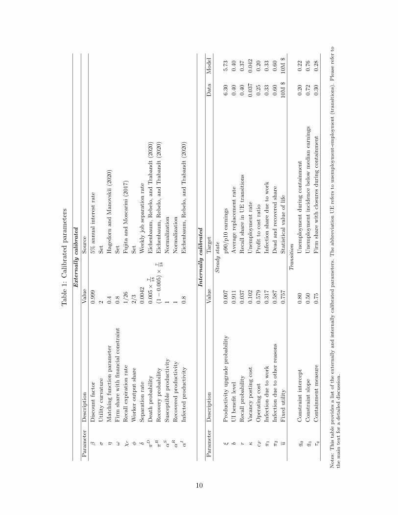
only government policy is the existing UI program. Table 1 summarizes the calibrated parameters.
Externally calibrated parameters. The model period is one week. The utility function is
given by u(c) = u+ c1−σ
1−σ as in Hall and Jones (2007), so that agents value life. We set σ = 2 and
discuss the calibration strategy for u below.
We assume a CES matching function, implying that the job finding rate is f(θ) = θ(1+θη)−1/η.
We set the matching function elasticity η to 0.4 (Hagedorn and Manovskii, 2008). We follow Gascon
(2020), who measures the employment share of essential occupations and those that can be done
remotely, and assign the essential sector an employment share of 54 percent. Furthermore, we
assume that 80 percent of the firms in the nonessential sector become financially constrained at the
onset of the epidemic (ω = 0.8). Fujita and Moscarini (2017) show that the probability of exiting
from unemployment through a recall approaches zero after six months of unemployment. This
requires setting the stochastic expiration rate of the recall option χr to 1/26. We set the worker’s
share of the output to φ = 2/3. Finally, we target a pre-COVID monthly separation rate of 1.65
percent computed using the Current Population Survey (CPS), and set δ to 0.0042.
To discipline the model’s SIR component, we follow Eichenbaum, Rebelo, and Trabandt (2020).
Assuming a mortality rate of 0.5 percent and that infected individuals either recover or die from
infection within 18 days, on average (πD + πR = 7/18), we obtain πD = 0.005 × 7/18 and πR =
(1− 0.005)× 7/18. Finally, we normalize the productivity of susceptible and recovered workers, αS
9
Tab
le1:
Cal
ibra
ted
par
amet
ers
Extern
allyca
libra
ted
Para
met
erD
escr
ipti
on
Valu
eSourc
e
βD
isco
unt
fact
or
0.9
99
5%
annual
inte
rest
rate
σU
tility
curv
atu
re2
Set
ηM
atc
hin
gfu
nct
ion
para
met
er0.4
Haged
orn
and
Manov
skii
(2020)
ωF
irm
share
wit
hfinanci
al
const
rain
t0.8
Set
χr
Rec
all
expir
ati
on
rate
1/26
Fuji
taand
Mosc
ari
ni
(2017)
φW
ork
eroutp
ut
share
2/3
Set
δSep
ara
tion
rate
0.0
042
Wee
kly
job
separa
tion
rate
πD
Dea
thpro
babilit
y0.0
05×
7 18
Eic
hen
baum
,R
ebel
o,
and
Tra
bandt
(2020)
πR
Rec
over
ypro
babilit
y(1
−0.0
05)×
7 18
Eic
hen
baum
,R
ebel
o,
and
Tra
bandt
(2020)
αS
Susc
epti
ble
pro
duct
ivit
y1
Norm
aliza
tion
αR
Rec
over
edpro
duct
ivit
y1
Norm
aliza
tion
αI
Infe
cted
pro
duct
ivit
y0.8
Eic
hen
baum
,R
ebel
o,
and
Tra
bandt
(2020)
Intern
allyca
libra
ted
Para
met
erD
escr
ipti
on
Valu
eT
arg
etD
ata
Model
Steadystate
ξP
roduct
ivit
yupgra
de
pro
babilit
y0.0
07
p90/p10
earn
ings
6.3
05.7
3
bU
Ib
enefi
tle
vel
0.9
11
Aver
age
repla
cem
ent
rate
0.4
00.4
0
rR
ecall
pro
babilit
y0.0
37
Rec
all
share
inU
Etr
ansi
tions
0.4
00.3
7
κV
aca
ncy
post
ing
cost
0.1
02
Unem
plo
ym
ent
rate
0.0
37
0.0
42
c FO
per
ati
ng
cost
0.5
79
Pro
fit
toco
stra
tio
0.2
50.2
0
π1
Infe
ctio
ndue
tow
ork
0.3
17
Infe
ctio
nsh
are
due
tow
ork
0.3
30.3
3
π2
Infe
ctio
ndue
tooth
erre
aso
ns
0.5
87
Dea
dand
reco
ver
edsh
are
0.6
00.6
0
uF
ixed
uti
lity
0.7
57
Sta
tist
ical
valu
eof
life
10M
$10M
$Transition
a0
Const
rain
tin
terc
ept
0.8
0U
nem
plo
ym
ent
duri
ng
conta
inm
ent
0.2
00.2
2
a1
Const
rain
tsl
op
e0.5
0U
nem
plo
ym
ent
inci
den
ceb
elow
med
ian
earn
ings
0.7
20.7
6
τ qC
onta
inm
ent
mea
sure
0.7
5F
irm
share
wit
hcl
osu
res
duri
ng
conta
inm
ent
0.3
00.2
8
Note
s:T
his
tab
lep
rovid
esa
list
of
the
exte
rnally
an
din
tern
ally
calib
rate
dp
ara
met
ers.
Th
eab
bre
via
tion
UE
refe
rsto
un
emp
loym
ent-
emp
loym
ent
(tra
nsi
tion
s).
Ple
ase
refe
rto
the
main
text
for
ad
etailed
dis
cuss
ion
.
10
and αR, to one and assume a 20 percent loss in productivity when infected, i.e., αI = 0.8.
Internally calibrated parameters. We calibrate eight of the remaining 11 parameters to match
steady-state moments of the U.S. economy prior to the pandemic and the remaining three by
simulating the COVID-19 pandemic and matching moments along the transition.
First, we discuss the steady-state moments. The probability ξ of a productivity upgrade for
actively producing a match has a pronounced effect on the earnings dispersion. Therefore, we target
the 90th to the 10th percentile ratio of the labor earnings distribution among employed workers,
which is 6.30 in the Survey of Program and Income Participation (SIPP).
Next, we target a replacement rate of 40 percent to discipline the UI payments b. The recall
probability r is chosen to match a 40 percent share of recalls in Unemployment-Employment (UE)
flows (Fujita and Moscarini, 2017).
Firms face two costs. We choose the vacancy posting cost κ to match an unemployment rate of
3.7 percent. Using aggregate income statements from the Internal Revenue Service (IRS), we find
that, in 2017, the ratio of profits to business expenses is around 25 percent for sole proprietorships.
We calibrate the fixed operating costs active firms incur cF to match this ratio.
We now describe the calibration of the parameters related to the epidemic. We choose π1 such
that the infections resulting from labor market activity account for one-third of all infections. To
pin down π2, we target a 60 percent combined share of recovered and dead individuals in a simple
SIR model with no behavioral response from households.10 Finally, because u governs how much
individuals value life over death, we choose u to match a statistical value of life of $10 million as
in Glover et al. (2020). Appendix A.3 provides more details.
Finally, we calibrate the remaining three parameters by simulating the COVID-19 pandemic
and matching moments along the transition. Specifically, we populate the economy with an initial
mass of 0.001 infected individuals.11 We assume that financial constraints in the nonessential sector
become operational and that the only government response is to implement a containment measure
τq in the nonessential sector during the first quarter of the pandemic.
The financial constraint is important for our substantive results, so we discuss its calibration
in more detail. The constraint depends linearly on productivity: a(z) = a0 + a1z. The constant a0
has a pronounced effect on the unemployment level during the epidemic. We choose this to match
a maximum unemployment rate of 20 percent for the first quarter of the epidemic.12 The slope of
the constraint, a1, determines which matches are predisposed to separation during the epidemic.
If a1 = 0, then wage rigidity implies that high-wage matches get destroyed. In contrast, a positive
10To do so, we simulate the system of equations given in Equation (A1) in Appendix A.1 under π1 = 0 and calculatethe total number of recovered and dead individuals in the steady state as a share of the initial population.
11We apportion this total initial infected mass to different labor market states, based on the population shares ofthe workers in the steady state.
12During the early stages of the shutdown in the U.S., there were many estimates of the peak unemployment ratein the absence of a policy response. Sahin, Tasci, and Yan (2020) estimated 16 percent; Treasury Secretary StevenMnuchin noted a peak of 25 percent; and Faria-e Castro (2020a) estimated 32.1 percent. In our baseline calibration,we take 20 percent as our target. Later, in Table 2, we also show the results when unemployment peaks at 35 percentunder stricter containment measures.
11
a1 makes low-wage matches more likely to dissolve. Since a1 determines the wage composition of
job losses, we choose it to match the incidence of the rise in unemployment across the earnings
distribution. Using the CPS, we divide occupations into employment-weighted earnings quantiles.
For each quantile, we calculate the change in temporary unemployment from January 2020 to April
2020. We find that occupations below the median of the earnings distribution account for 72 percent
of the total increase in temporary unemployment.13 We target this moment to discipline a1.
Finally, we choose the strictness of the containment policy τq to match the fraction of businesses
with temporary closings during the pandemic. According to the Small Business Pulse Survey of
the U.S. Census Bureau, the fraction of businesses that temporarily closed for at least one day
during any week of May 2020 was around 30 percent. We map temporary closings to firms pausing
production in the model and calculate the fraction of idle matches in the nonessential sector.
4 Results
We now analyze the effects of an epidemic under various labor market policies. We start with
a baseline containment of τq = 0.75 and no accompanying fiscal support, which we compare to
two extreme cost-equivalent options: channel all additional transfers either through UI or through
payroll subsidies. We then solve for the optimal mix of these policies and consider how this mix
changes with the strictness of the containment. In all our experiments, we assume that policies are
introduced coincident with the epidemic’s onset and that they last for one quarter (13 weeks).14
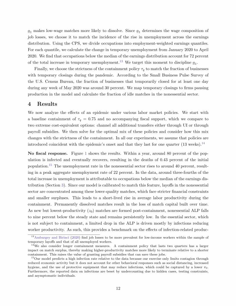
No fiscal response. Figure 1 shows the results. Within a year, around 80 percent of the pop-
ulation is infected and eventually recovers, resulting in the deaths of 0.43 percent of the initial
population.15 The unemployment rate in the nonessential sector rises to around 40 percent, result-
ing in a peak aggregate unemployment rate of 22 percent. In the data, around three-fourths of the
total increase in unemployment is attributable to occupations below the median of the earnings dis-
tribution (Section 3). Since our model is calibrated to match this feature, layoffs in the nonessential
sector are concentrated among these lower-quality matches, which face stricter financial constraints
and smaller surpluses. This leads to a short-lived rise in average labor productivity during the
containment. Permanently dissolved matches result in the loss of match capital built over time.
As new but lowest-productivity (z0) matches are formed post-containment, nonessential ALP falls
to nine percent below the steady state and remains persistently low. In the essential sector, which
is not subject to containment, a limited drop in the ALP is driven mostly by infections reducing
worker productivity. As such, this provides a benchmark on the effects of infection-related produc-
13Amburgey and Birinci (2020) find job losses to be more prevalent for low-income workers within the sample oftemporary layoffs and that of all unemployed workers.
14We also consider longer containment measures. A containment policy that lasts two quarters has a largerimpact on match surplus, thereby making higher-productivity matches more likely to terminate relative to a shortercontainment. This raises the value of granting payroll subsidies that can save these jobs.
15Our model predicts a high infection rate relative to the data because our exercise only limits contagion throughreduced economic activity but it does not account for other behavioral responses such as social distancing, increasedhygiene, and the use of protective equipment that may reduce infections, which could be captured by a lower π2.Furthermore, the reported data on infections are beset by undercounting due to hidden cases, testing constraints,and asymptomatic individuals.
12
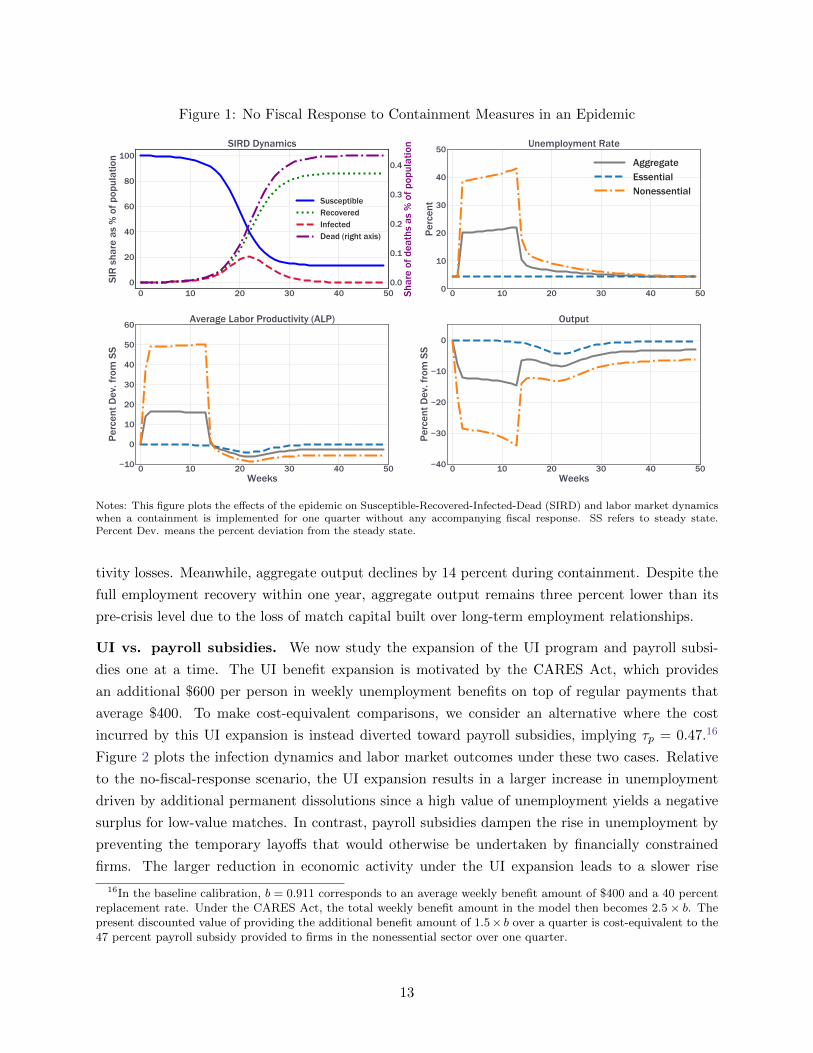
Figure 1: No Fiscal Response to Containment Measures in an Epidemic
0 10 20 30 40 500
20
40
60
80
100
SIR
sha
re a
s %
of p
opul
atio
n
SIRD Dynamics
SusceptibleRecoveredInfectedDead (right axis)
0 10 20 30 40 500
10
20
30
40
50
Perc
ent
Unemployment Rate
AggregateEssentialNonessential
0 10 20 30 40 50Weeks
10
0
10
20
30
40
50
60
Perc
ent D
ev. f
rom
SS
Average Labor Productivity (ALP)
0 10 20 30 40 50Weeks
0
10
20
30
40
Perc
ent D
ev. f
rom
SS
Output
0.0
0.1
0.2
0.3
0.4
Shar
e of
dea
ths
as %
of p
opul
atio
n
Notes: This figure plots the effects of the epidemic on Susceptible-Recovered-Infected-Dead (SIRD) and labor market dynamicswhen a containment is implemented for one quarter without any accompanying fiscal response. SS refers to steady state.Percent Dev. means the percent deviation from the steady state.
tivity losses. Meanwhile, aggregate output declines by 14 percent during containment. Despite the
full employment recovery within one year, aggregate output remains three percent lower than its
pre-crisis level due to the loss of match capital built over long-term employment relationships.
UI vs. payroll subsidies. We now study the expansion of the UI program and payroll subsi-
dies one at a time. The UI benefit expansion is motivated by the CARES Act, which provides
an additional $600 per person in weekly unemployment benefits on top of regular payments that
average $400. To make cost-equivalent comparisons, we consider an alternative where the cost
incurred by this UI expansion is instead diverted toward payroll subsidies, implying τp = 0.47.16
Figure 2 plots the infection dynamics and labor market outcomes under these two cases. Relative
to the no-fiscal-response scenario, the UI expansion results in a larger increase in unemployment
driven by additional permanent dissolutions since a high value of unemployment yields a negative
surplus for low-value matches. In contrast, payroll subsidies dampen the rise in unemployment by
preventing the temporary layoffs that would otherwise be undertaken by financially constrained
firms. The larger reduction in economic activity under the UI expansion leads to a slower rise
16In the baseline calibration, b = 0.911 corresponds to an average weekly benefit amount of $400 and a 40 percentreplacement rate. Under the CARES Act, the total weekly benefit amount in the model then becomes 2.5 × b. Thepresent discounted value of providing the additional benefit amount of 1.5× b over a quarter is cost-equivalent to the47 percent payroll subsidy provided to firms in the nonessential sector over one quarter.
13
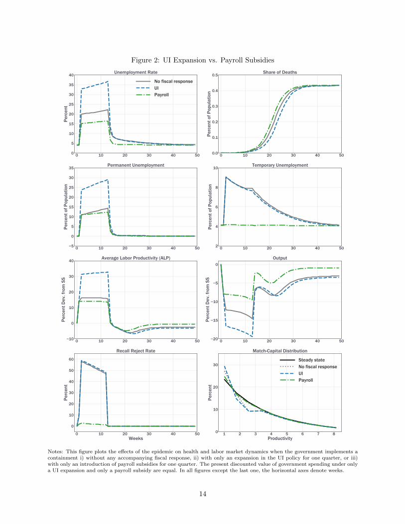
Figure 2: UI Expansion vs. Payroll Subsidies
0 10 20 30 40 500
5
10
15
20
25
30
35
40
Perc
ent
Unemployment Rate
No fiscal responseUIPayroll
0 10 20 30 40 500.0
0.1
0.2
0.3
0.4
0.5
Perc
ent o
f Pop
ulat
ion
Share of Deaths
0 10 20 30 40 505
0
5
10
15
20
25
30
35
Perc
ent o
f Pop
ulat
ion
Permanent Unemployment
0 10 20 30 40 502
4
6
8
10
Perc
ent o
f Pop
ulat
ion
Temporary Unemployment
0 10 20 30 40 5010
0
10
20
30
40
Perc
ent D
ev. f
rom
SS
Average Labor Productivity (ALP)
0 10 20 30 40 50
0
5
10
15
20
Perc
ent D
ev. f
rom
SS
Output
0 10 20 30 40 50Weeks
0
10
20
30
40
50
60
Perc
ent
Recall Reject Rate
1 2 3 4 5 6 7 8Productivity
0
10
20
30
Perc
ent
Match-Capital Distribution
Steady stateNo fiscal responseUIPayroll
Notes: This figure plots the effects of the epidemic on health and labor market dynamics when the government implements acontainment i) without any accompanying fiscal response, ii) with only an expansion in the UI policy for one quarter, or iii)with only an introduction of payroll subsidies for one quarter. The present discounted value of government spending under onlya UI expansion and only a payroll subsidy are equal. In all figures except the last one, the horizontal axes denote weeks.
14
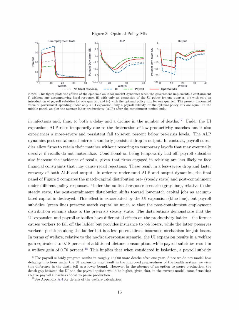
Figure 3: Optimal Policy Mix
0 10 20 30 40Weeks
0
10
20
30
40
Perc
ent
Unemployment Rate
15 20 30 40Weeks
10.0
7.5
5.0
2.5
0.0
2.5
5.0
Perc
ent D
ev. f
rom
SS
ALP
0 10 20 30 40Weeks
25
20
15
10
5
0
5
Perc
ent D
ev. f
rom
SS
Output
No fiscal response UI Payroll Optimal Mix
Notes: This figure plots the effects of the epidemic on labor market dynamics when the government implements a containmenti) without any accompanying fiscal response, ii) with only an expansion of the UI policy for one quarter, iii) with only anintroduction of payroll subsidies for one quarter, and iv) with the optimal policy mix for one quarter. The present discountedvalue of government spending under only a UI expansion, only a payroll subsidy, or the optimal policy mix are equal. In themiddle panel, we plot the average labor productivity (ALP) after the containment period ends.
in infections and, thus, to both a delay and a decline in the number of deaths.17 Under the UI
expansion, ALP rises temporarily due to the destruction of low-productivity matches but it also
experiences a more-severe and persistent fall to seven percent below pre-crisis levels. The ALP
dynamics post-containment mirror a similarly persistent drop in output. In contrast, payroll subsi-
dies allow firms to retain their matches without resorting to temporary layoffs that may eventually
dissolve if recalls do not materialize. Conditional on being temporarily laid off, payroll subsidies
also increase the incidence of recalls, given that firms engaged in rehiring are less likely to face
financial constraints that may cause recall rejections. These result in a less-severe drop and faster
recovery of both ALP and output. In order to understand ALP and output dynamics, the final
panel of Figure 2 compares the match-capital distribution pre- (steady state) and post-containment
under different policy responses. Under the no-fiscal-response scenario (gray line), relative to the
steady state, the post-containment distribution shifts toward low-match capital jobs as accumu-
lated capital is destroyed. This effect is exacerbated by the UI expansion (blue line), but payroll
subsidies (green line) preserve match capital so much so that the post-containment employment
distribution remains close to the pre-crisis steady state. The distributions demonstrate that the
UI expansion and payroll subsidies have differential effects on the productivity ladder—the former
causes workers to fall off the ladder but provides insurance to job losers, while the latter preserves
workers’ positions along the ladder but is a less-potent direct insurance mechanism for job losers.
In terms of welfare, relative to the no-fiscal-response scenario, the UI expansion results in a welfare
gain equivalent to 0.18 percent of additional lifetime consumption, while payroll subsidies result in
a welfare gain of 0.76 percent.18 This implies that when considered in isolation, a payroll subsidy
17The payroll subsidy program results in roughly 15,000 more deaths after one year. Since we do not model howdelaying infections under the UI expansion may result in the improved preparedness of the health system, we viewthis difference in the death toll as a lower bound. However, in the absence of an option to pause production, thedeath gap between the UI and the payroll options would be higher, given that, in the current model, some firms thatreceive payroll subsidies choose to pause production.
18See Appendix A.4 for details of the welfare calculation.
15

Figure 4: Match-Capital Distribution
1 2 3 4 5 6 7 8Productivity
0
10
20
30
Perc
ent
Steady stateNo fiscal responseUI
1 2 3 4 5 6 7 8Productivity
0
10
20
30Steady statePayrollOptimal Mix
Notes: This figure plots the pre-containment (steady state) and post-containment (seven weeks after the containment) match-capital distribution. The post-containment distributions are shown separately for the following scenarios: i) having no fiscalresponse, ii) only expanding UI benefits, iii) only introducing payroll subsidies, and iv) implementing the optimal policy mix.
is preferred over a cost-equivalent UI expansion.
Optimal mix of policies. What is the optimal policy mix? Given a baseline containment rate of
τq = 0.75, we solve for b and τp to maximize welfare subject to preserving the cost equivalence with
the preceding exercise. The optimal policy prescribes an 80 percent budget allocation toward UI
while the remaining 20 percent is spent on payroll subsidies, yielding a welfare gain of 0.85 percent in
additional lifetime consumption relative to a no-fiscal-response alternative. This implies b∗ = 2.20
and τ∗p = 0.10. The left-hand column of Figure 3 shows that under the optimal policy, the relatively
generous UI payments induce a large increase in unemployment, more than halfway between the
no-fiscal-response and the full-UI scenarios. However, the 10 percent payroll subsidy goes a long
way toward preserving match capital, as evidenced by the less-severe drop in ALP. An important
implication is that even if the unemployment rate is drastically higher under the optimal policy
(red) relative to having no fiscal response (gray), the output during containment is the same and
recovers much faster under the optimal policy. The faster recovery occurs because firm-worker pairs
with high match capital resume production once the containment period ends. This is supported by
the left-hand column of Figure 4, where the match-capital distribution significantly worsens under
both no fiscal response (gray) and full UI (blue), but the optimal policy with only τ∗p = 0.1 (red)
is capable of preserving match capital close to steady-state levels and, importantly, accomplishes
what a large payroll subsidy of τp = 0.47 (green) would have achieved. This brings us to two
important conclusions. First, a payroll subsidy that is just enough to prevent high-productivity
matches from dissolving eliminates the need for generous subsidies in excess of what firms need
to weather the containment period. Second, UI and payroll subsidies target workers on different
rungs of the productivity ladder. On the one hand, payroll subsidies seek to preserve matches
for highly productive workers and prevent their flow into unemployment. On the other hand,
for less-productive matches predisposed to dissolution even with payroll subsidies, UI serves as an
16
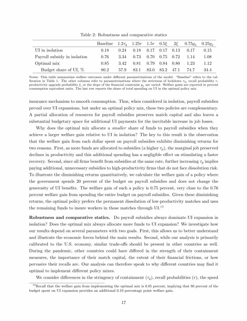
Table 2: Robustness and comparative statics
Baseline 1.2τq 1.25r 1.5r 0.5ξ 2ξ 0.75a1 0.25a1
UI in isolation 0.18 0.24 0.18 0.17 0.17 0.13 0.17 0.15
Payroll subsidy in isolation 0.76 3.34 0.73 0.70 0.75 0.72 1.14 1.08
Optimal mix 0.85 3.42 0.81 0.79 0.84 0.80 1.23 1.12
Budget share of UI, % 80.2 57.9 83.1 83.0 83.2 47.1 74.7 34.4
Notes: This table summarizes welfare outcomes under different parametrizations of the model. “Baseline” refers to the cal-ibration in Table 1. The other columns refer to parameterizations where the strictness of lockdown τq , recall probability r,productivity upgrade probability ξ, or the slope of the financial constraint a1 are varied. Welfare gains are reported in percentconsumption equivalent units. The last row reports the share of total spending on UI in the optimal policy mix.
insurance mechanism to smooth consumption. Thus, when considered in isolation, payroll subsidies
prevail over UI expansions, but under an optimal policy mix, these two policies are complementary.
A partial allocation of resources for payroll subsidies preserves match capital and also leaves a
substantial budgetary space for additional UI payments for the inevitable increase in job losses.
Why does the optimal mix allocate a smaller share of funds to payroll subsidies when they
achieve a larger welfare gain relative to UI in isolation? The key to this result is the observation
that the welfare gain from each dollar spent on payroll subsidies exhibits diminishing returns for
two reasons. First, as more funds are allocated to subsidies (a higher τp), the marginal job preserved
declines in productivity and this additional spending has a negligible effect on stimulating a faster
recovery. Second, since all firms benefit from subsidies at the same rate, further increasing τp implies
paying additional, unnecessary subsidies to high-productivity firms that do not face dissolution risk.
To illustrate the diminishing returns quantitatively, we calculate the welfare gain of a policy where
the government spends 20 percent of the budget on payroll subsidies and does not change the
generosity of UI benefits. The welfare gain of such a policy is 0.75 percent, very close to the 0.76
percent welfare gain from spending the entire budget on payroll subsidies. Given these diminishing
returns, the optimal policy prefers the permanent dissolution of low-productivity matches and uses
the remaining funds to insure workers in those matches through UI.19
Robustness and comparative statics. Do payroll subsidies always dominate UI expansion in
isolation? Does the optimal mix always allocate more funds to UI expansion? We investigate how
our results depend on several parameters with two goals. First, this allows us to better understand
and illustrate the economic forces behind the main results. Second, while our analysis is primarily
calibrated to the U.S. economy, similar trade-offs should be present in other countries as well.
During the pandemic, other countries could have differed in the strength of their containment
measures, the importance of their match capital, the extent of their financial frictions, or how
pervasive their recalls are. Our analysis can therefore speak to why different countries may find it
optimal to implement different policy mixes.
We consider differences in the stringency of containment (τq), recall probabilities (r), the speed
19Recall that the welfare gain from implementing the optimal mix is 0.85 percent, implying that 80 percent of thebudget spent on UI expansion provides an additional 0.10 percentage point welfare gain.
17
of learning on the job (ξ), and how financial frictions vary across firms with different productivities
(a1). For each exercise, we compute the welfare gain of introducing either a UI expansion or a
payroll subsidy in isolation as well as the new optimal policy mix and its associated welfare gain.
To ensure comparability, we choose the policy parameters τp and b such that the policies are cost-
equivalent with the baseline. In the case of financial frictions, we also recalibrate a0 to obtain the
same peak unemployment as in our baseline. Our results are summarized in Table 2.
Under a stricter lockdown (1.2τq), the no-fiscal-response scenario induces a higher peak unem-
ployment rate (35 percent) and causes the dissolution of an even wider range of highly productive
matches, thereby generating a larger decline in ALP and output (Figure A1 in Appendix A.5).
Similar to the main exercise, allocating the entire budget to UI expansion exacerbates these effects
because strict containment greatly depresses the surplus from high-productivity matches. There-
fore, the optimal policy now prescribes less-generous UI benefits. Specifically, the optimal mix
now allocates a lower fraction, 58 percent, of the budget on UI. The optimal policy significantly
alleviates the drop in productivity and output, even during containment (Figure A1), and preserves
the high-productivity matches that would otherwise have dissolved (Figure A2). As a result, the
welfare gain from the optimal mix becomes much larger under strict containment. Once again, we
note that the 42 percent budget allocation on payroll subsidies captures most of the gains that
allocating the entire budget to payroll would have achieved (Figure A2).
A higher recall probability ensures that a lower share of temporary layoffs results in permanent
match destruction and reduces the potential benefit of payroll subsidies. This effect is quantitatively
small: A 25 or even 50 percent higher r reduces the budget share allocated to payroll subsidies in
the optimal mix from 20 percent to 17 percent. There are three reasons for why a higher recall
probability results in only a modest decline in the share of spending on payroll subsidies: i) contain-
ment measures induce negative surpluses for some matches, leading to permanent separations that
recalls cannot remedy, ii) productivity stagnates during temporary separations prior to recalls, and
iii) a higher recall probability reduces but does not completely eliminate the permanent expiration
of the recall option and the severance of ties between workers and firms.
The rate at which productivity grows on the job (ξ) is an important determinant of the optimal
policy. We discipline this parameter by targeting the wage dispersion in the data. An alternative
approach is to target the earnings losses upon job loss because ξ controls how much wages grow
among job stayers relative to job losers. Reassuringly, our model does a good job in matching the
initial earnings loss while understating losses in the longer term by about 5 percentage points (see
Appendix A.6). Regardless of the fit, our estimate for ξ may be biased upward. This is because the
inequality and the consequences of job loss in the data are shaped by a host of factors apart from
differences in the match productivity alone. To gauge the robustness of our conclusions, we solve
for the optimal policy by setting ξ to double that of the baseline value and then to half the baseline
value. Raising ξ by a factor of two makes long-tenure matches much more productive, thereby
increasing the benefit of payroll subsidies. Consequently, the optimal policy allocates 53 percent
of the budget to this component. Conversely, lowering ξ dictates a lower share to be allocated
18
to payroll subsidies, given the reduced importance of match-specific capital. In isolation, payroll
subsidies still provide a much larger welfare gain relative to a cost-equivalent UI expansion.
Another important aspect is the relationship between financial frictions and match productivity
governed by a1. Whether constraints bind more for high- or low-productivity firms is important
for the policy tradeoff. A lower a1 implies a tighter constraint for high-productivity matches.
When these output-critical jobs are more predisposed to permanent dissolution, match preservation
through payroll subsidies becomes more important. We find that reducing a1 down to a quarter
of its baseline value increases the optimal spending on payroll subsidies to a level that is twice the
proportion spent on UI. However, such a low value for a1 implies that separations from low-paying
jobs (below the median wage) account for only 11 percent of the total increase in unemployment.
This number is clearly at odds with the 72 percent share observed in the data, which is an integral
part of how we discipline the distribution of job losses in our model.
5 Conclusion
The COVID-19 pandemic and the ensuing policy interventions to contain it have had unprecedented
negative effects on the U.S. labor market. In response, the U.S. government implemented two types
of labor market policies: expanding UI payments and granting payroll subsidies to vulnerable firms.
In this paper, we study the usefulness of these policies, both in isolation and in conjunction. The
introduction of payroll subsidies alone is preferred over a cost-equivalent UI expansion as it preserves
highly productive matches during containment, thus enabling a faster recovery of productivity and
output following the lifting of containment measures. When considered jointly, however, a cost-
equivalent optimal mix allocates 20 percent of the budget to payroll subsidies and 80 percent to UI
expansion. This allocation is sufficient to save high-productivity jobs from dissolution, while the
remaining funds are used to provide income to less-productive workers who face inevitable job loss.
We abstract away from two potentially important margins. First, we assume away labor mobility
across sectors. If the pandemic has a disproportionately persistent effect on labor demand in one
of the sectors, then policies that tie workers to jobs, such as payroll subsidies, would become
less desirable. Second, we abstract away from welfare gains due to demand stabilization. Because
payroll subsidies and UI policies benefit different groups of people with potentially different marginal
propensities to consume, their effects on aggregate demand may be different. We leave these
important considerations for future research.
References
Alon, T., M. Doepke, J. Olmstead-Rumsey, and M. Tertilt (2020): “This time it’s different: The
role of women’s employment in a pandemic recession,” Tech. rep., National Bureau of Economic Research.
Alvarez, F. E., D. Argente, and F. Lippi (2020): “A simple planning problem for covid-19 lockdown,”
Tech. rep., National Bureau of Economic Research.
Amburgey, A. and S. Birinci (2020): “Which earnings groups have been most affected by the COVID-19
crisis?” Economic Synopses.
19
Atkeson, A. (2020): “What will be the economic impact of Covid-19 in the US? Rough estimates of disease
scenarios,” Tech. rep., National Bureau of Economic Research.
Berger, D. W., K. F. Herkenhoff, and S. Mongey (2020): “An seir infectious disease model with
testing and conditional quarantine,” Tech. rep., National Bureau of Economic Research.
Bick, A. and A. Blandin (2020): “Real time labor market estimates during the 2020 coronavirus out-
break,” Unpublished Manuscript, Arizona State University.
Birinci, S. (2020): “Spousal labor supply response to job displacement and implications for optimal trans-
fers,” Tech. rep., Federal Reserve Bank of Saint Louis.
Birinci, S. and K. See (2020): “How should unemployment insurance vary over the business cycle?” Tech.
rep., Federal Reserve Bank of St. Louis.
Boar, C. and S. Mongey (2020): “Dynamic trade-offs and labor supply under the CARES Act,” Tech.
rep., National Bureau of Economic Research.
Brotherhood, L., P. Kircher, C. Santos, and M. Tertilt (2020): “An economic model of the Covid-
19 pandemic with young and old agents: Behavior, testing and policies,” Tech. rep., University of Bonn
and University of Mannheim, Germany.
Burdett, K. and R. Wright (1989): “Unemployment insurance and short-time compensation: The
effects on layoffs, hours per worker, and wages,” Journal of Political Economy, 97, 1479–1496.
Cahuc, P., F. Kramarz, S. Nevoux, et al. (2018): “When short-time work works,” Tech. rep., Sciences
Po Departement of Economics.
Chodorow-Reich, G., J. Coglianese, and L. Karabarbounis (2019): “The macro effects of unem-
ployment benefit extensions: a measurement error approach,” The Quarterly Journal of Economics, 134,
227–279.
Cooper, R., M. Meyer, and I. Schott (2017): “The employment and output effects of short-time work
in Germany,” Tech. rep., National Bureau of Economic Research.
Davis, S. J. and T. von Wachter (2011): “Recessions and the Costs of Job Loss,” Brookings Papers on
Economic Activity, 1.
Eichenbaum, M. S., S. Rebelo, and M. Trabandt (2020): “The macroeconomics of epidemics,” Tech.
rep., National Bureau of Economic Research.
Fang, L., J. Nie, and Z. Xie (2020): “Unemployment insurance during a pandemic,” Tech. rep., Federal
Reserve Bank of Atlanta.
Faria-e Castro, M. (2020a): “Back-of-the-envelope estimates of next quarter’s unemployment rate,” Saint
Louis Fed Blogs.
——— (2020b): “Fiscal policy during a pandemic,” FRB St. Louis Working Paper.
Fujita, S. and G. Moscarini (2017): “Recall and unemployment,” American Economic Review, 107,
3875–3916.
Ganong, P., P. J. Noel, and J. S. Vavra (2020): “US unemployment insurance replacement rates
during the pandemic,” Tech. rep., National Bureau of Economic Research.
Garriga, C., R. Manuelli, and S. Sanghi (2020): “Optimal management of an epidemic: Lockdown,
vaccine and value of life,” Tech. rep., Federal Reserve Bank of St. Louis.
Gascon, C. (2020): “COVID-19: Which workers face the highest unemployment risk?” St. Louis
Fed On the Economy, https://www. stlouisfed. org/on-the-economy/2020/march/covid-19-workers-highest-
unemployment-risk.
Giupponi, G. and C. Landais (2020): “Subsidizing labor hoarding in recessions: The employment &
welfare effects of short time work,” Working paper.
20
Glover, A., J. Heathcote, D. Krueger, and J.-V. Rıos-Rull (2020): “Health versus wealth: On
the distributional effects of controlling a pandemic,” Tech. rep., National Bureau of Economic Research.
Gregory, V., G. Menzio, and D. G. Wiczer (2020): “Pandemic recession: L or V-shaped?” Tech. rep.,
National Bureau of Economic Research.
Hagedorn, M., F. Karahan, I. Manovskii, and K. Mitman (2019): “Unemployment benefits and
unemployment in the great recession: the role of macro effects,” Tech. rep., National Bureau of Economic
Research.
Hagedorn, M. and I. Manovskii (2008): “The cyclical behavior of equilibrium unemployment and
vacancies revisited,” American Economic Review, 98, 1692–1706.
Hall, R. E. and C. I. Jones (2007): “The value of life and the rise in health spending,” The Quarterly
Journal of Economics, 122, 39–72.
Jacobson, L. S., R. J. LaLonde, and D. G. Sullivan (1993): “Earnings losses of displaced workers,”
American economic review, 685–709.
Jarosch, G. (2015): “Searching for job security and the consequences of job loss,” Tech. rep., Princeton
University.
Jung, P. and K. Kuester (2015): “Optimal labor-market policy in recessions,” American Economic
Journal: Macroeconomics, 7, 124–56.
Kapicka, M. and P. Rupert (2020): “Labor markets during pandemics,” Manuscript, UC Santa Barbara.
Kermack, W. O. and A. G. McKendrick (1927): “A contribution to the mathematical theory of
epidemics,” Proceedings of the royal society of london. Series A, Containing papers of a mathematical and
physical character, 115, 700–721.
Kolsrud, J., C. Landais, P. Nilsson, and J. Spinnewijn (2018): “The optimal timing of unemployment
benefits: Theory and evidence from Sweden,” American Economic Review, 108, 985–1033.
Krusell, P., T. Mukoyama, and A. Sahin (2010): “Labour-market matching with precautionary savings
and aggregate fluctuations,” The Review of Economic Studies, 77, 1477–1507.
Kurmann, A., E. Lale, and L. Ta (2020): “The impact of COVID-19 on U.S. employment and hours:
Real-time estimates with homebase data,” Tech. rep., Drexel University.
Landais, C., P. Michaillat, and E. Saez (2018): “A macroeconomic approach to optimal unemployment
insurance: Applications,” American Economic Journal: Economic Policy, 10, 182–216.
Mitman, K. and S. Rabinovich (2015): “Optimal unemployment insurance in an equilibrium business-
cycle model,” Journal of Monetary Economics, 71, 99–118.
——— (2020): “Optimal unemployment benefits in the pandemic,” Tech. rep., IZA Discussion Papers.
Nakajima, M. (2012): “A quantitative analysis of unemployment benefit extensions,” Journal of Monetary
Economics, 59, 686–702.
Sahin, A., M. Tasci, and J. Yan (2020): “The unemployment cost of COVID-19: How high and how
long?” Economic Commentary.
Stevens, A. H. (1997): “Persistent effects of job displacement: The importance of multiple job losses,”
Journal of Labor Economics, 15, 165–188.
Tilly, J. and K. Niedermayer (2016): “Employment and welfare effects of short-time work,” Tech. rep.,
Working paper.
21
A Appendix
A.1 Stationary Equilibrium
Let s ∈ {E,N} denote the essential E and nonessential N sectors. A recursive equilibrium for
this economy is a list of household and firm policy functions for whether to keep an existing match
dhW,k,s, dhUT ,k,k′,s
, and dhJ,k,s; whether to produce or pause lhs , ∀h ∈ {S, I,R}, ∀s ∈ {E,N}, and
∀k ∈ {C,U}; labor market tightness θs ∀s ∈ {E,N}; an aggregate law of motion for the mass
of susceptible S, infected I, recovered R, and dead D agents; and the distribution of households
across states µ such that,
1. given government policies, household and firm policy functions solve their problems;
2. labor market tightness in sector s satisfies the free-entry condition V = 0;
3. the aggregate laws of motion for health status are given by
St+1 = St − TtIt+1 = It + Tt −
(πR + πD
)It
Rt+1 = Rt + πRIt
Dt+1 = Dt + πDIt,
(A1)
where the total number of new infections in period t is Tt = π1NSt N
It + π2StIt and Nh is the
total number of actively employed households with health status h; and
4. µ is the invariant distribution implied by contact rates in the labor market, transition matrices
of health status Πn and of match-specific productivity P , and household and firm decision
rules.
A.2 Computational Details
In this section, we describe how we solve and simulate our model.
A.2.1 Steady State
We use value function iteration to solve for worker and firm optimization problems. The algorithm
we use to obtain the stationary equilibrium of the model is outlined below.
For a given parameterization of the model and for each sector s ∈ {E,N}, perform the following:
1. Start with an initial guess for the value of market tightness θs0.
2. For each guess of θsn in iteration n:
(a) Iterate over the worker and firm value functions in Equations (2), (3), (6), (7) and (8)
until convergence.
(b) Iterate on the model-implied laws of motion in order to compute for the stationary
worker distribution over employment states, health status and productivity.
22
(c) Solve the market tightness level θsn+1 that satisfies the free-entry condition V = 0, where
V is given in Equation (9). We then calculate its absolute deviation from θsn.
(d) If the deviation is less than a tolerance level, then we stop. Otherwise we update the
guess for market tightness to θsn+1 = ζθn+ (1− ζ)θsn+1 with dampening parameter ζ < 1
and return to Step 2.
A.2.2 Transition
For each policy, in calculating the impulse responses, we focus on perfect foresight transition dynam-
ics following one-time and unanticipated shocks out of the steady state, using a shooting algorithm
as outlined below.
1. Fix the number of time periods it takes to reach the new steady state, T .
2. Compute the initial (no-infection) steady-state equilibrium for a given set of model parameters
according to the algorithm in Section A.2.1. As the epidemic is transitory and there is no
permanent productivity difference between susceptible and recovered workers, the worker and
firm value functions in the terminal steady state are the same as in the initial steady state as
is the labor market tightness for each sector.
3. Guess a sequence of infected workers’ labor supply and the total number of infected in the
economy as a whole, {N I,0t , I0
t }T−1t=1 . For each sector s ∈ {E,N}:
(a) Guess a sequence of labor market tightness {θs,0t }T−1t=1 .
(b) Solve for the path of worker and firm value functions for t ∈ {1, . . . , T − 1} backwards,
given the shocks, path of infection {N I,0t , I0
t }T−1t=1 , market tightness {θs,0t }
T−1t=1 , and ter-
minal worker and firm values in period T .
(c) Compute the sequence of labor market tightness {θs,1t }T−1t=1 that is consistent with the
free-entry condition and the laws of motion for workers over the state space induced by
the decisions implied by the path of value functions over t ∈ {1, . . . , T − 1}.
(d) Check whether max1≤t<T |θs,1t − θs,0t | is less than some tolerance level. If yes, continue;
if not, update {θs,0t }T−1t=1 and go back to Step (b).
(e) Check whether |θs,1T − θs,0T | is less than some tolerance level. If yes, then stop; if not,
then increase T and go back to Step 1.
4. Calculate the sequence of infected workers’ labor supply and the total number of infected
workers, {N I,1t , I1
t }T−1t=1 , which is implied by the path of the worker distribution over the
transition.
5. Check whether max1≤t<T |N I,1t −N
I,0t | and max1≤t<T |I1
t − I0t | are less than some tolerance
level. If yes, then continue; if not, then update {N I,0t }
T−1t=1 and {I0
t }T−1t=1 and return to Step 3.
6. Check whether |N I,1T − N I,0
T | and |I1T − I0
T | are less than some tolerance level. If yes, then
stop; if not, then increase T and go back to Step 1.
23
A.3 Computing the Statistical Value of Life
To calculate the model-implied statistical value of life (SVL), we first compute the fraction
of lifetime consumption π all agents in the steady-state economy are willing to forgo in order to
prevent a rise in the probability of death by ψ = 110,000 . We do this by resolving our no-infection
model with a discount factor β = (1− ψ)β that is adjusted by this mortality rate and finding the
π that renders workers indifferent between these two economies behind the veil of ignorance.
Second, to convert the fraction π to a dollar amount, we take the quarterly consumption amount
from the National Income Accounts. U.S. consumption per capita in the fourth quarter of 2019 was
$40, 748. We divide this number by 52.14 to arrive at a weekly consumption of cNIPAw = $781.5. The
model-implied weekly dollar amount that workers are willing to forgo is then given by π × cNIPAw .
In the final step, we convert the weekly consumption that workers are willing to forgo into a
present value term by taking its geometric sum; i.e. πcNIPAw1−β . This implies that the total amount
that workers are willing to pay to avoid one death is 1ψπcNIPAw
1−β , which is the definition of SVL. We
choose the constant u in the utility function such that SV L = $10M .
A.4 Computing Welfare
To compute a welfare metric, we solve for the percent change in lifetime consumption π that
renders a household behind the veil of ignorance indifferent between the baseline economy and the
economy under a new labor market policy, accounting for all policy changes during the transition
period. The expected value of a particular policy p when that policy is implemented, is given by
EV (π, p) ≡T−1∑t=1
βt−1
[∫u ((1 + π) cit(p)) dΛit(p)
]+ βT−1
∫ViT (π, p)dΛiT (p),
where cit(p) denotes the consumption of individual i under policy p in period t, Λit(p) is the
cross-sectional cumulative density function of workers, and ViT (π, p) is the steady-state value of
individual i, where they receive an additional π percent of their consumption under that policy.
The underlying assumption here is that the economy is close enough to its terminal steady state by
the end of period T . In practice, we choose T = 500 weeks in our computations, which we observe
to be long enough for the economy to have converged to a stationary equilibrium.
Finally, to arrive at the welfare metric π(p) under policy p, we solve the following condition:
EV (π, 0) = EV (0, p),
where we use the convention that p = 0 denotes the baseline economy: i.e., there are no fiscal
measures introduced. Otherwise, we consider p ∈ {UI,Payroll,Mix} for various policy scenarios.
A.5 Additional Results on the Baseline vs the Stricter Containment Measures
Below, we elaborate on the effects of stricter containment measures and how an optimal policy
mix with more weight on payroll subsidies alleviates its economic burden.
As discussed in Section 4, increasing the strength of containment measures from τq = 0.75 by
24
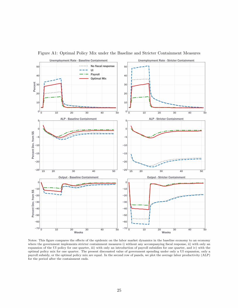
Figure A1: Optimal Policy Mix under the Baseline and Stricter Containment Measures
0 10 20 30 40 500
10
20
30
40
50
Perc
ent
Unemployment Rate - Baseline Containment
No fiscal responseUIPayrollOptimal Mix
0 10 20 30 40 500
10
20
30
40
50
Unemployment Rate - Stricter Containment
15 20 30 40 5025
20
15
10
5
0
5
Perc
ent D
ev. f
rom
SS
ALP - Baseline Containment
15 20 30 40 5025
20
15
10
5
0
5ALP - Stricter Containment
0 10 20 30 40 50Weeks
70
60
50
40
30
20
10
0
Perc
ent D
ev. f
rom
SS
Output - Baseline Containment
0 10 20 30 40 50Weeks
70
60
50
40
30
20
10
0
Output - Stricter Containment
Notes: This figure compares the effects of the epidemic on the labor market dynamics in the baseline economy to an economywhere the government implements stricter containment measures i) without any accompanying fiscal response, ii) with only anexpansion of the UI policy for one quarter, iii) with only an introduction of payroll subsidies for one quarter, and iv) with theoptimal policy mix for one quarter. The present discounted value of government spending under only a UI expansion, only apayroll subsidy, or the optimal policy mix are equal. In the second row of panels, we plot the average labor productivity (ALP)for the period after the containment ends.
25
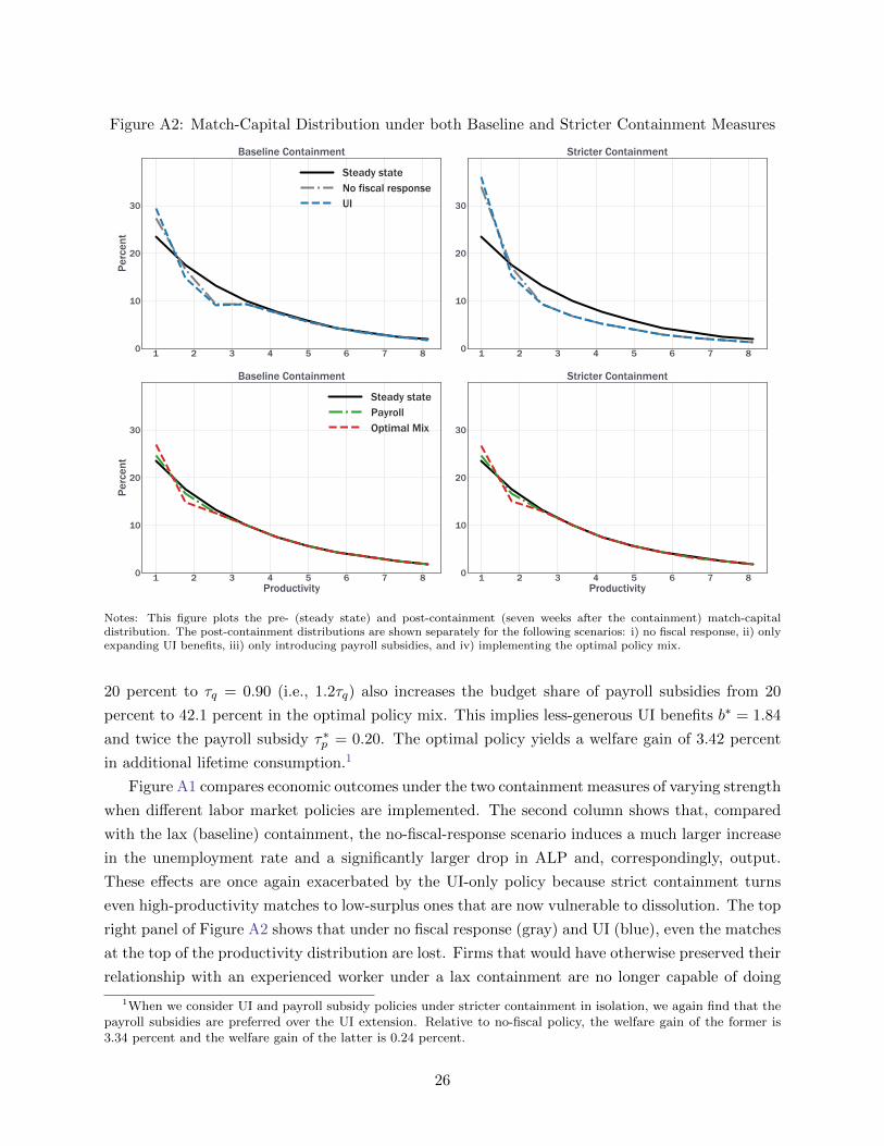
Figure A2: Match-Capital Distribution under both Baseline and Stricter Containment Measures
1 2 3 4 5 6 7 80
10
20
30
Perc
ent
Baseline Containment
Steady stateNo fiscal responseUI
1 2 3 4 5 6 7 80
10
20
30
Stricter Containment
1 2 3 4 5 6 7 8Productivity
0
10
20
30
Perc
ent
Baseline Containment
Steady statePayrollOptimal Mix
1 2 3 4 5 6 7 8Productivity
0
10
20
30
Stricter Containment
Notes: This figure plots the pre- (steady state) and post-containment (seven weeks after the containment) match-capitaldistribution. The post-containment distributions are shown separately for the following scenarios: i) no fiscal response, ii) onlyexpanding UI benefits, iii) only introducing payroll subsidies, and iv) implementing the optimal policy mix.
20 percent to τq = 0.90 (i.e., 1.2τq) also increases the budget share of payroll subsidies from 20
percent to 42.1 percent in the optimal policy mix. This implies less-generous UI benefits b∗ = 1.84
and twice the payroll subsidy τ∗p = 0.20. The optimal policy yields a welfare gain of 3.42 percent
in additional lifetime consumption.1
Figure A1 compares economic outcomes under the two containment measures of varying strength
when different labor market policies are implemented. The second column shows that, compared
with the lax (baseline) containment, the no-fiscal-response scenario induces a much larger increase
in the unemployment rate and a significantly larger drop in ALP and, correspondingly, output.
These effects are once again exacerbated by the UI-only policy because strict containment turns
even high-productivity matches to low-surplus ones that are now vulnerable to dissolution. The top
right panel of Figure A2 shows that under no fiscal response (gray) and UI (blue), even the matches
at the top of the productivity distribution are lost. Firms that would have otherwise preserved their
relationship with an experienced worker under a lax containment are no longer capable of doing
1When we consider UI and payroll subsidy policies under stricter containment in isolation, we again find that thepayroll subsidies are preferred over the UI extension. Relative to no-fiscal policy, the welfare gain of the former is3.34 percent and the welfare gain of the latter is 0.24 percent.
26
so under strict containment. Thus, the optimal policy now prescribes a larger payroll subsidy
(τ∗p = 0.2). The bottom right panel of Figure A2 shows that the match quality distribution under
the optimal policy (red) approaches the pre-crisis distribution, while a full-payroll subsidy (green)
yields only marginal gains. As a result, the optimal policy significantly alleviates the drop in
productivity and output even during containment, which is the reason why the welfare gain from
the optimal mix becomes much higher under strict containment. Once again, we note that the
40 percent budget allocation to payroll subsidies captures most of the gains that a full budget
allocation to payroll would have achieved, as shown in the bottom right panel of Figure A2.
A.6 Earnings Drop upon Job Loss
To estimate the consequences of job loss for individual earnings, we follow Jacobson et al.
(1993) and Stevens (1997) and use a distributed lag regression. We first simulate a weekly panel
of workers from the steady-state equilibrium of the model. Next, to compare between the existing
empirical estimates and their model counterparts, we aggregate the model’s weekly data into an
annual frequency. Finally, we run the following regression on model-generated annual data:
yit =20∑
k≥−5
ψkDkit + αi + εit. (A2)
Here, yit denotes the labor earnings of individual i in year t and αi captures individual fixed effects.
The vector of dummy variables Dkit indicates an individual’s job loss in a future, current, or previous
year.2 For example, D5it = 1 if individual i lost a job in year t− 5 and zero otherwise.
We estimate ψk for the five years preceding the job loss (k = −5,−4,−3,−2,−1), for the year
of the job loss (k = 0), and for every year until 20 years after the job loss (k = 1, 2, ..., 20). Here, ψk
captures the effect on the year t earnings of individuals who are displaced k years before/after year
t (treatment group). The control group consists of individuals who never experience displacement
over the estimation period. Thus, individuals in the control group have Dkit = 0 for all years t.
In our results below, the earnings drop upon job loss measures the change in the earnings of the
treatment group relative to the change in the earnings of the control group. Finally, we report the
estimated earnings losses ψk as a percent of the mean earnings in the year prior to the job loss.
Figure A3 compares the model’s predictions with the empirical estimates obtained by Jarosch
(2015). Two main points are worth highlighting.
First, even though the baseline calibration does not target the earnings drop upon job loss,
its magnitude (35 percent) in the year following the job loss is remarkably close to the data (37
percent), at least to that measured in Jarosch (2015), who uses administrative data from Germany
to estimate a specification similar to Equation (A2). For the U.S., our estimate is smaller than the
estimate in Jacobson et al. (1993) (40 percent) and larger than that in Stevens (1997) (30 percent).
Moreover, Davis and von Wachter (2011) and Birinci (2020) estimate the earnings drop upon job
2We obtain yearly earnings by summing weekly earnings. If an individual loses a job for at least one week in ayear, then we set the job loss dummy to one for that year.
27

Figure A3: Earnings dynamics upon job loss: Data vs model
5 0 5 10 15 20Years from job loss
40
30
20
10
0
Perc
ent c
hang
e
DataModelModel 0.5Model 2
Notes: This figure plots the earnings dynamics upon job loss. The model results are obtained by estimating a distributed lagregression on the annual data that is simulated from the model. The three series correspond to the following cases: i) thebaseline calibration (dashed blue line), ii) the economy with the productivity upgrade probability ξ of half the baseline value(dotted blue line), and iii) the economy with ξ twice the baseline value (dash-dotted blue line). The empirical estimates areobtained from Jarosch (2015).
loss separately for recessions and expansions. Using administrative data from the U.S., Davis
and von Wachter (2011) find larger earnings losses upon displacement in recessions (39 percent)
than in expansions (25 percent). Similarly, using the Panel Study of Income Dynamics, Birinci
(2020) finds an earnings drop of 39 percent in recessions and 22 percent in expansions in the year
following the job loss. To sum up, our model implies an estimate of the earnings drop upon job
loss that is within the range of existing estimates for recessions and expansions. That being said,
the longer-term effects are understated by around 5 percentage points compared to the data.
Second, we recognize that while the magnitude and persistence of the earnings drop upon job
loss in the model are not too far off the data, these losses in the model are entirely due to match-
specific capital, whereas in the data they may also be driven by losses in other forms of human
capital (general, occupation-specific, etc.), employer stigma, and so on. In order to understand
how differences in the importance of match-specific capital map to the optimal policy, in Section 4
we conduct a robustness analysis on ξ. This parameter is the probability that match productivity
increases on the job and therefore controls how important match-specific capital is. We consider
two alternative values for this parameter: half (0.5ξ) and double the baseline (2ξ) values. Figure
A3 shows that as ξ increases, the earnings drop upon job loss becomes more severe, both in the
short- and long-term. This result arises because a large ξ implies faster productivity growth for
the control group over the period during which job losers remain unemployed.
28