Labor Market Frictions and Optimal Steady-State Inflation∗

Mikael Carlsson†and Andreas Westermark‡

February 26, 2014

Abstract

In central theories of monetary non-neutrality, the Ramsey optimal steady-state inflation rate

varies between the negative of the real interest rate and zero. This paper explores how the in-

teraction of nominal wage and search and matching frictions affect the policy prescription. The

mechanism we have in mind arises in a model with search frictions when nominal wages are not

continuously rebargained and some newly hired workers enter into an existing wage structure. We

show that adding the combination of such frictions to the canonical monetary model can generate

an optimal inflation rate that is significantly positive. Specifically, for a standard U.S. calibration,

we find a Ramsey optimal inflation rate of 115 percent per year, as compared to a rate of −076percent when wages for new hires are fully flexible.

Keywords: Optimal Monetary Policy, Inflation, Labor Market Frictions.

JEL classification: E52, H21, J60.

∗We are grateful to the editor Antonella Triagari, an anonymous referee, Roberto Billi, Tore Ellingsen, Michael Krause,Per Krusell, Lars E.O. Svensson, Karl Walentin and participants at the Greater Stockholm Macro Group, JLS Seminar

Series, Frankfurt, and the EEA Congress in Oslo, 2011, for useful comments and discussions. The views expressed in this

paper are solely the responsibility of the authors and should not be interpreted as reflecting the views of the Executive

Board of Sveriges Riksbank.†Uppsala University, Uppsala Center for Labor Studies and Sveriges Riksbank. E-mail: mikael.carlsson@nek.uu.se.‡Research Department, Sveriges Riksbank, SE-103 37, Stockholm, Sweden. e-mail: andreas.westermark@riksbank.se.

1

1 Introduction

In leading theories of monetary non-neutrality, the policy prescription for the optimal steady-state

inflation rate varies between the negative of the real interest rate (the Friedman rule) and zero (price

stability); see Schmitt-Grohe Uribe, 2010, for an overview. In this paper we explore a new channel

where the interaction of nominal wage and labor market search and matching frictions affects the

planner’s trade-off between the welfare costs and benefits of inflation. We show that the combination

of such frictions can in fact generate a Ramsey optimal inflation rate that is significantly positive.

Importantly, this is the case even in the presence of a monetary friction, which drives the optimal

inflation rate towards the Friedman rule of deflation.

The mechanism we have in mind arises in a model with search frictions when nominal wages are

not continuously rebargained and some newly hired workers enter into an existing wage structure.1 In

this case, we show in a stylized model that inflation not only affects real-wage profiles over a contract

spell, but also redistributes surplus between workers and firms, since incumbent workers impose an

externality on new hires through the entry wage. Specifically, this affects the wage-bargaining outcome

through the workers’ outside option and hence the expected present value of total labor costs for a

match as well as firms’ incentives for vacancy creation. We derive a Hosios condition for the stylized

model and show that the Ramsey planner has incentives to increase inflation if employment and

vacancy creation are inefficiently low in order to push the economy towards the efficient allocation.

Thus, in an efficient allocation, as in Thomas (2008), this incentive vanishes (and the reverse occurs

when employment is inefficiently high). Also, the Ramsey planner loses the ability to affect real-wage

costs via inflation if all new workers get to rebargain their wage. In this case, the full effect of inflation

on entry wages is internalized in the wage bargain, and firm and worker surpluses, as well as real wage

costs, become neutral to inflation. This is also the case if search frictions vanish since the Ramsey

planner loses any leverage over vacancy/job creation. Thus, models without an extensive margin on

the labor market lack the mechanism described here (as e.g. in Erceg, Henderson and Levin, 2000).

Overall, the key insight from the stylized model is that if both search and wage-setting externalities

are present, there is an incentive for the Ramsey planner to vary the inflation rate to increase welfare

through its effect on job creation and unemployment.

To quantitatively evaluate the relative strength of this mechanism, we introduce it into a full-fledged

1Data supports that a non-negligible share of newly hired workers enter into an existing wage structure. First, micro-

data evidence on wages does not indicate that wages are more sensitive to labor market conditions at the beginning than

later in the span of a match (once the variation in the composition of firms and match quality over the cycle is controlled

for); see Gertler and Trigari (2009). Secondly, survey evidence, like Bewley (1999), Bewley (2007) for the U.S. and the

study performed within the Eurosystem Wage Dynamics Network (WDN), reported by Galuscak, Keeney, Nicolitsas,

Smets, Strzelecki, and Vodopivec (2012), present strong evidence that the wages of new hires are tightly linked to those

of incumbents.

2

model encompassing leading theories of monetary non-neutrality. The model we outline features a non-

Walrasian labor market with search frictions as in Mortensen and Pissarides (1994), Trigari (2009)

and Christoffel, Kuester, and Linzert (2009). Moreover, there are impediments to continuous resetting

of nominal prices and wages modeled along the lines of Dotsey, King, and Wolman (1999), where

adjustment probabilities are endogenous. Finally, the model features a role for money as a medium of

exchange, as in Khan, King, and Wolman (2003) and Lie (2010).

In the quantitative model, variation in the average inflation rate will have several effects on wel-

fare. First, inflation will affect the opportunity cost of holding money, pushing the optimal inflation

rate towards the Friedman rule. Second, because of monopolistic competition and nominal frictions,

inflation causes relative price distortions, which drive the optimal inflation rate towards zero. Finally,

we introduce the mechanism presented above, i.e., search frictions combined with new hires entering

into an existing wage structure, where the inflation rate affects equilibrium real-wage costs and, in

turn, job creation.

In a standard U.S. calibration of the model, implying that employment is 187 percentage points

lower than in the efficient allocation, we find that the Ramsey optimal inflation rate is 115 percent

per year. Moreover, varying the share of new hires receiving rebargained wages has a substantial effect

on the optimal inflation rate. If all newly hired workers receive rebargained wages, thus shutting down

the interaction effect between nominal wage frictions and search and matching frictions, the optimal

inflation rate is −076 percent.2 When none [50 percent, the baseline] (all, as in Gertler and Trigari(2009)), of the newly hired workers enter into an existing wage structure, the optimal inflation rate

is −076 [115] (135) percent. Thus, only a moderate share of new workers entering into an existingwage structure is needed to obtain a significantly positive optimal inflation rate.

When shutting down the monetary distortion and looking at the cashless economy, as analyzed in

Woodford (2003), we find that the Ramsey optimal inflation rate increases to 152 percent. Thus, the

monetary distortion has a moderately negative effect on the optimal policy prescription.

The results reported above are conditional on agents optimally choosing when to change prices

and wages. It is then interesting to study the effect of shutting down the endogenous response of

the adjustment probabilities to variations in inflation and let the agents face a fixed adjustment

hazard. In contrast to Lie (2010), we find that endogenizing adjustment probabilities matters for

the quantitative analysis. Specifically, exogenous price and wage adjustment hazards give a Ramsey

optimal inflation rate of 295 percent, thus an increase of almost two percentage points relative to the

2This is the same rate as if we let all wage contracts be continuously rebargained in the model (not only those of the

new hires). These cases are the same due to the fact that wages are not allocative in the search-matching framework

we rely on, or more specifically, a relative-wage dispersion across firms does not give rise to a dispersion of labor supply

across individuals working at different firms.

3

case with endogenous adjustment hazards.

All in all, we find that the combination of search and wage-setting externalities within the canonical

monetary model introduces an important link between inflation and welfare and hence potentially a

large difference in prescribed policy.

For clarity, the quantitative model outlined in this paper does not encompass all mechanisms

that can affect the Ramsey optimal steady-state inflation rate. Papers studying the effect of other

mechanisms on the Ramsey optimal steady-state inflation are Schmitt-Grohé and Uribe (2010) using

inflation as an indirect tax to address tax evasion, Schmitt-Grohé and Uribe (2012a) analyzing foreign

demand of domestic currency, Schmitt-Grohé and Uribe (2012b) studying quality bias, Adam and Billi

(2006) and Billi (2011) looking into the effect of the zero lower bound, and Kim and Ruge-Murcia

(2011) addressing downward nominal wage rigidity.3 Of these, only a substantial foreign demand of

domestic currency and a planner that only cares about the well-being of the home country may lead

to a significantly positive inflation rate. Moreover, all of these features are, if anything, likely to drive

up the Ramsey optimal steady-state inflation rate. Thus, in this sense the results presented here can

be viewed as a lower bound.

This paper is outlined as follows: In section 2 we present the basic mechanism we have in mind,

in section 3, we outline the framework for the quantitative evaluation, including a description of the

optimal Ramsey policy, in section 4 the calibration and the quantitative results are presented. Finally,

section 5 concludes.

2 The Mechanism

To set ideas, it is helpful to first focus on a stylized stationary equilibrium model of the labor market

featuring the interaction mechanism we have in mind.4 Let firms and workers sign contracts with

a fixed (nominal) wage, , that with certainty lasts for two periods. Letting denote the price

level in the first period of the contract and the gross inflation rate, the real wage in the first and

second periods of the contract, respectively, are then = and 0 =

=

. This captures the first

component we need, i.e. nominal wage frictions. We restrict attention to the case where gross inflation

is positive, i.e., 0. Secondly, we assume that there are search and matching frictions captured

by a constant returns matching function, giving rise to a surplus to be bargained over. Specifically,

we assume that the number of matches, , is given by the constant-returns matching function in

3There is also a literature focusing on the dynamic effects of labor market frictions under the Ramsey optimal policy;

see Faia (2008, 2009) and Faia and Rossi (2013).4We are grateful to Antonella Trigari for suggesting how to substantially improve this section.

4

Den Haan, Ramey, and Watson (2000);

=

( + )1

(1)

where is unemployment and vacancies. The probability that a worker is matched to a firm is

=

(2)

and the probability that a vacancy is filled is

=

(3)

We denote the surplus of the firm (worker) () with ∈ 0 1 where = 0 denotes that the wageis rebargained and = 1 that the wage is not rebargained. The surplus for the firm in a period when

wages are rebargained is then

0 = − + 1 (4)

where is the (real) marginal revenue for the firm, is the discount factor and is the fixed

probability that the match survives into the next period. Moreover, in a period when the wage is not

rebargained the, surplus is

1 = −

+ 0 (5)

Similarly, the surpluses for the worker are

0 = − + £1 −

¤(6)

1 =

− +

£0 −

¤ (7)

where is (real) income received when unemployed, financed via lump-sum taxes, the probability

of finding a job and the average value of being employed across all firms in the economy. Note

that variations in affect the workers’ outside option in the bargain. All renegotiating firms set the

same wage and the wage path for a rebargaining firm is

(8)

and for a non-rebargaining firm, the wage path is

(9)

5

The output, denoted by , is sold at price and is used as input by final-good firms that produce

using a constant returns technology = , facing CES demand with elasticity as in equation

(41) below. This implies that is the marginal cost of final-goods firms which in equilibrium is

= −1

1. Note, however, that the social value of an additional employed worker is equal to unity

due to the constant returns technology. The planner solution can be described by5

1− () =+ () −

(12)

where is the vacancy posting cost, is the probability of filling a vacancy, = is tightness and

() = −

, i.e. the elasticity of the job-finding probability w.r.t. to tightness, together with the

unemployment transition equation.6

Case 1: Flexible Wages

In a competitive equilibrium, labor market variables are determined by job creation and bargaining.

Firm and worker values are

0 = − + 0 (13)

0 = − + £0 −

¤

where = 0 in this case. From job creation, we have

= 0 (14)

where

0 = −

1− (15)

From wage setting, via Nash bargaining, we have

(1− )0 = 0 (16)

5This follows from solving the planner problem as in Pissarides (2000) p. 184-185 for a discrete economy. Formally,

social welfare is ∞=0

(1 (1− )− ) (10)

and unemployment evolves according to

1− = (1− −1) + −1−1−1 (11)

Solving the optimization problem then gives expression (12) in steady state.6Note that if the matching function is Cobb-Douglas, () is a constant and equal to the elasticity of the matching

function w.r.t. unemployment.

6

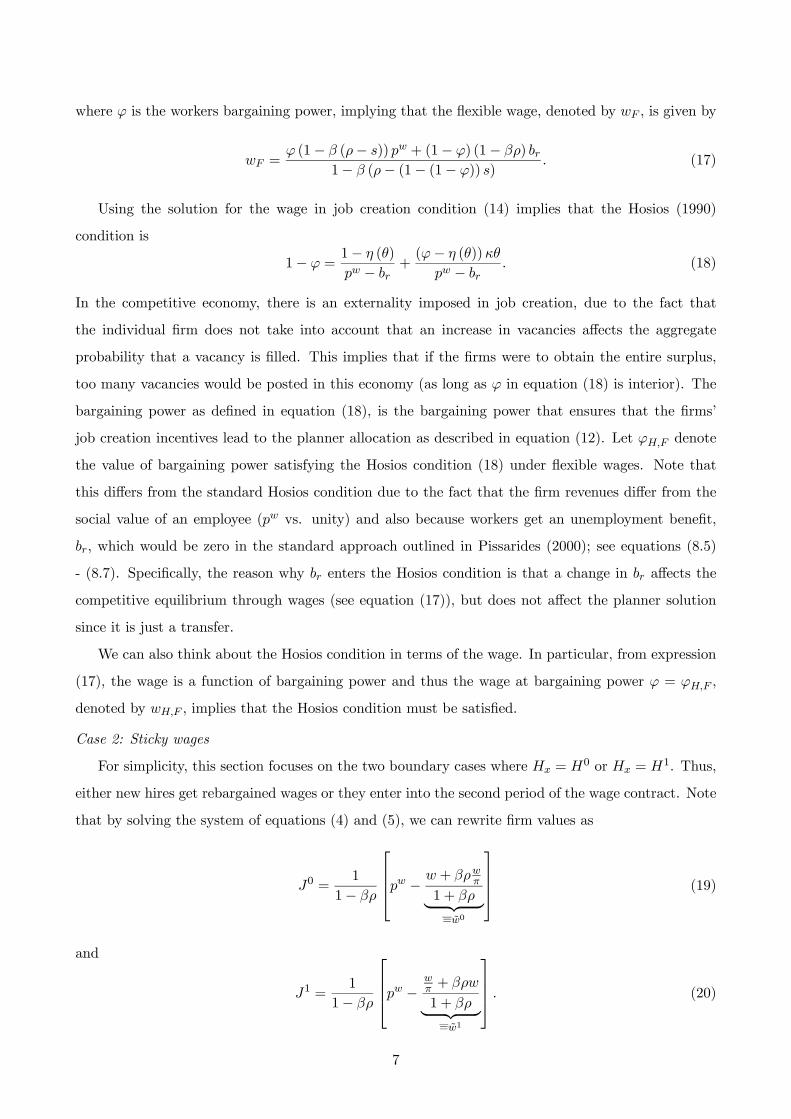
where is the workers bargaining power, implying that the flexible wage, denoted by , is given by

= (1− (− )) + (1− ) (1− )

1− (− (1− (1− )) ) (17)

Using the solution for the wage in job creation condition (14) implies that the Hosios (1990)

condition is

1− =1− ()

− +(− ())

− (18)

In the competitive economy, there is an externality imposed in job creation, due to the fact that

the individual firm does not take into account that an increase in vacancies affects the aggregate

probability that a vacancy is filled. This implies that if the firms were to obtain the entire surplus,

too many vacancies would be posted in this economy (as long as in equation (18) is interior). The

bargaining power as defined in equation (18), is the bargaining power that ensures that the firms’

job creation incentives lead to the planner allocation as described in equation (12). Let denote

the value of bargaining power satisfying the Hosios condition (18) under flexible wages. Note that

this differs from the standard Hosios condition due to the fact that the firm revenues differ from the

social value of an employee ( vs. unity) and also because workers get an unemployment benefit,

, which would be zero in the standard approach outlined in Pissarides (2000); see equations (8.5)

- (8.7). Specifically, the reason why enters the Hosios condition is that a change in affects the

competitive equilibrium through wages (see equation (17)), but does not affect the planner solution

since it is just a transfer.

We can also think about the Hosios condition in terms of the wage. In particular, from expression

(17), the wage is a function of bargaining power and thus the wage at bargaining power = ,

denoted by , implies that the Hosios condition must be satisfied.

Case 2: Sticky wages

For simplicity, this section focuses on the two boundary cases where = 0 or = 1. Thus,

either new hires get rebargained wages or they enter into the second period of the wage contract. Note

that by solving the system of equations (4) and (5), we can rewrite firm values as

0 =1

1−

⎡⎢⎢⎣ − +

1 + | z =0

⎤⎥⎥⎦ (19)

and

1 =1

1−

⎡⎢⎢⎣ − +

1 + | z =1

⎤⎥⎥⎦ (20)

7

Similarly, from the system of equations (6) and (7),

0 =1

1−

£0 − ( + )

¤ (21)

1 =1

1−

£1 − ( + )

¤ (22)

Nash bargaining (16) implies that, when renegotiating, the parties share the surplus so that the present

value of the wage sequence shares the present value of surpluses according to the bargaining power

and we get

0 = + (1− ) ( + ) (23)

where superscript = denotes when = 0 and = 1, respectively. That is 0 is the

wage when all new hires get a rebargained wage and 0 is the wage when all new hires enter into

an old contract. In the latter case, the present value of the wage sequence is lower when 1, since

the worker first gets the deflated wage and then the rebargained wage . Furthermore, the higher

the inflation rate, the lower the present value of wages when new hires enter into an existing contract

relative to in a renegotiated match. We denote this ratio by

()=10

=1+

1 + 1

(24)

for = . Note also that 0 () 0, lim→0 () = 1, (1) = 1 and lim→∞ () = .

Using (6), (7) and (23) gives

0 =1− (− )

1− (− (1− (1− )) )

∙ + (1− )

1−

1− (− )

¸(25)

and

0 =1− (− )

1− (− (1− (1− ) ()) )

∙ + (1− )

1−

1− (− )

¸ (26)

Note that whenever 1 and hence () 1 the wage when new hires get rebargained wages is

higher than when new hires enter into an existing wage structure, i.e. 0 0. The reason for this is

that employed workers take into account that an increase in inflation affect the wage profile for their

own contract and hence adjust accordingly, but they do not take into consideration the effect the

wage profile has on the entry wages of new hires, i.e. . Thus, incumbent (bargaining) workers

impose an externality on the entry wage of new hires. This, in turn, leads to a lowering of the present

value of the wage sequence for new hires (see equation (9)), and in turn to a worsening of the outside

option for workers when bargaining and a reduction in the equilibrium wage. Relying on the same

8

notation, note also that job creation is

= 0 (27)

when = 0 and

= 1 (28)

when = 1. Thus, it is the wages of newly hired workers (0 and 1) that matters for equilibrium

outcomes (echoing Pissarides, 2009).

Now consider the relationship to the flexible wage economy and the Hosios condition. First, when

= 0, note that 0 = . Hence, the firm surplus 0 in equation (27) is the same as in the

economy with flexible wages (see equation (15)). This in turn implies that job creation, employment

and unemployment are the same and = . Moreover, the Hosios condition is again described

as in equation (18).

Second, if = 1 when 1 we have 0 0 since 1 and when 1 we have 0 0 .

Focusing on the case where 1, the equilibrium present value of wages in a non-renegotiating match

1 does not share the surplus according to the bargaining power , but instead gives the firm a higher

share of the surplus than what would be implied by its bargaining power. Also, from (19) - (21) the

total surplus for new matches is

1

1−

£ − ¡ + 0

¢¤(29)

when = 0 and

1

1−

£ − ¡ + 1

¢¤(30)

when = 1. Since 0 =

0−1−(−) 1

=()1−1−(−) , the total surplus for new matches is larger

when = 1 than when = 0. Thus, when new hires get non-renegotiated wages, the firm gets

a larger share of a larger surplus, both of which increase the firm value of a new hire. Formally,

1 = − () 0

1− 0 =

− 01−

(31)

implying that firms will post more vacancies than in the case where new workers get rebargained

wages. Hence, employment will be higher and unemployment lower. Furthermore, by subtracting and

adding 0 in the numerator for the value of 1 in equation (31), using

0 = and proceeding as

in the flexible wage case, the Hosios condition is

1− =1− ()

− − ()−

− − 1− +

(1− ) ( − )

¡0 − () 0

¢ (32)

where the first two terms on the right-hand side are as in equation (18), but the last term is new and

9

is due to the fact that the wage paid to new hires is different from the wage in equation (25) (and

thus the wage in equation (17)). Let denote the value of satisfying the above equation.

Note that equation (32) depends on . Then, in contrast to the flexible wage case and the case

where new hires get new wages, there are several values of for which the planner solution can be

implemented by an appropriate choice of . To see this, first note that, using 0 in (28) and that

and are functions of (using the CRS property of the matching function), the job creation condition

(28) implicitly determines equilibrium tightness as a function of and . Denote this function by

= ( ), which is decreasing in .7 The equilibrium wage costs (1 in equation (20)) paid by

hiring firms is

1 ( ) = 1− (− ( ( )))

1− (− (1− (1− ) ) ( ( )))(33)

×∙ + (1− )

1−

1− (− ( ( )))

¸

which is increasing in , again by using (28). Since is in the open set ( 1) and since 1 ( ) is

increasing in , the set of feasible wages, =( ), is open where the lower and upper bounds

are =1 () and =

1 (1 ), respectively. Furthermore, as → 1 both the upper

and lower bounds converge to . Whether ∈ or not determines if the planner solution

can be achieved. Note first that when = the planner solution can be implemented by setting

= 1, implying () = 1 and hence 1¡1

¢= and . Second, since

the bounds are continuous in , we have ∈ for close to implying that there is a

∈ (0∞) that implements the planner solution.8 Third, if or the planner

solution can not be implemented and the policymaker has incentives to either create hyper inflation

( →∞) or hyper deflation ( → 0) depending on which boundary is relevant.9 Thus, there is a set

of values for the bargaining power

Ω =© ∈ [0 1] | ∃ ∈ ( 1) s.t. 1 ( ) =

ª (34)

where the planner solution can be implemented by appropriately choosing .

Recall that the Ramsey planner chooses inflation subject to the constraints from private sector

behavior. Then it follows from above that the Ramsey optimal inflation rate either does not exist

7This follows from differentiating (28).8Here we do not consider a subsidy to intermediate goods production or as instruments for the Ramsey policy

maker. For a discussion on tax-policy implementation of the first-best allocation in a model with nominal rigidities and

labor market frictions see Ravenna and Walsh (2012).9That the planner solution can not be implemented for some parameter values follows from noting that when

we have 1 (1 ) and, if we in addition let → 1, we also have .

10

or is the rate that implements the planner solution in (12). Below we develop a richer model adding

additional frictions for the Ramsey planner to consider when designing optimal policy (i.e., price

adjustment frictions and money demand). These frictions introduce additional trade-offs that eliminate

the nonexistence problems associated with hyper inflation/deflation. Specifically, price adjustment

tends to push the Ramsey optimal inflation rate to zero, while the Friedman rule tends to push it

towards the negative of the real interest rate.

Note also that, if search frictions vanish, i.e., when the job finding probability → 1, due to

→ 0, the competitive equilibrium converges to the planner solution. To see this, note that the

planner solution has → 0 and → 1 when → 0.10 In the competitive economy, the equilibrium

also has → 0 and → 1 in the case where → 0.11 This follows from that the surplus of a match

1 is strictly positive and hence we have → 0 from equation (28), in turn implying → 1.12 Thus,

when search frictions vanish, the competitive equilibrium allocation converges to the planner solution,

eliminating any incentives to use the mechanism above.13

The key insight here is that if both search and wage-setting externalities are present, this mech-

anism is active. In this case, a Ramsey planner has incentives to vary the inflation rate in order to

increase welfare through its effect on equilibrium wages through , in turn affecting job creation and

unemployment.

In relation to earlier literature it is first worth noting that this mechanism is not at work in Thomas

10To see this, note first that

=1

(1 + )1

(35)

=1

1 + − 1

(36)

and

() =

1 + (37)

The planner optimality condition can be written as

(1− ) =1

(1 + )1

+1

1−

+1 (38)

Then, as → 0, we have →∞ and hence → 0 and → 1.11As long as there is not too much deflation.12To see this, note first that we can write

1 =

( )

(1− ) (1− (− (1− (1− ) ) )) (39)

where 0 for 1 and ∈ [0 1]. Also, for 1, is decreasing in . Note also that the denominator is always

positive. Consider the equilibrium for diffferent values of and let be defined by 1= 0. Then, for all ,

since ( ) 0 for all ∈ [0 1], we have → 0 from equation (28) when → 0 and in turn → 1. For we

instead have → max () 1 when → 0, where max () is the value of that solves ( ) = 0. Then equilibrium

tightness, denoted by max, is determined by using equation (36). This, in turn, determines from equation (35).13For the case of too much deflation, the entry wage 1 ( ) is larger than the gross surplus, for job finding rates

close to one. Then the limit equilibrium job finding probability is instead the value of where 1 = 0 leading to an

inefficient outcome.

11

(2008) due to the fact that the calibration implies that the Hosios condition holds and hence that there

are no steady-state search externalities. Moreover, the model of Erceg, Henderson, and Levin (2000)

does not feature this mechanism either. This is due to the fact that there is no extensive margin on

the labor market in that model and hence no room for search frictions. Thus, the Ramsey planner

has no leverage on job creation through the channel outlined above. However, and similarly to our

model, the Erceg, Henderson, and Levin (2000) model features a markup in wage-setting where the

actual markup can be different from the flexible price markup because of Calvo (1983)-style wage

stickiness. Thus, in both models the planner has incentives to tilt the real-wage profile in order to

lower the actual markup and increase labor input.14 Note though, since the model lacks a leverage on

job creation there is much less of a motive for the planner to use this channel as shown by Amano,

Moran, Murchison, and Rennison (2009).15 The model in Kim and Ruge-Murcia (2011) is similar to

Amano, Moran, Murchison, and Rennison (2009), but differs in that it instead relies on wage-setting

frictions along the lines of Rotemberg (1982). This, however, does not seem to be important for the

Ramsey optimal inflation rate.16

3 A Model for Quantitative Evaluation

The next step in our analysis attempts to realistically evaluate the quantitative importance of the

mechanism outlined above by embedding it in the canonical monetary model. The basic framework

for the quantitative evaluation shares many elements of standard models. There is a monopolistically

competitive intermediate goods sector where producers set prices facing a stochastic fixed adjustment

cost as in Dotsey, King, and Wolman (1999). The intermediate goods sector buys a homogenous input

from the wholesale sector, which, in turn, uses labor in the production of this input. The market for

this homogenous input is characterized by perfect competition.

In contrast to previous papers studying the Ramsey optimal steady-state inflation rate, our model

features search and matching frictions and staggered wage bargaining. Specifically, the wholesale

sector posts vacancies on a search and matching labor market similar to Christoffel, Kuester, and

Linzert (2009) and Trigari (2009). Wages are bargained between a representative family and wholesale

firms in a setting with stochastic impediments to rebargaining, akin to how price setting is modeled.

The representative family construct, composed of many workers as in Merz (1995), is introduced

14The average wage markup in an EHL model is computed in equation (16) in Amano, Moran, Murchison, and

Rennison (2009).15 In Table 1 of Amano, Moran, Murchison, and Rennison (2009), the optimal inflation rate (without productivity

growth) is 003%. Since only taking into account markup variations across households would imply an optimal inflation

rate of zero, the effect of using inflation to affect the average markups in the economy is tiny.16The paper by Kim and Ruge-Murcia (2011) has its focus on downward nominal wage rigidities, which is not the

focus here. However, they also look at the case with symmetric wage adjustment frictions and find a deflation rate of

about 0.1 percent. Thus, their result is very much in line with Amano, Moran, Murchison, and Rennison (2009).

12

to ensure complete consumption insurance. The representative family then supplies labor, bargains

wages and assures equal consumption across workers within the family. Finally, notation is simplified

by assuming a flexible-price retail sector that repacks the intermediate goods in accordance with

consumer preferences and sells them to the representative family on a competitive market. We also

add a monetary friction along the lines of Dotsey, King, and Wolman (1999).

3.1 Intermediate-Goods Firms

The intermediate-goods firm chooses whether to adjust prices or not. Let the probability of adjusting

prices in a given period be denoted by , given that the firm last adjusted its price periods ago.

For technical reasons, we assume that there is some 1 such that −1 = 1. Note that we follow

standard notation and label the cohorts from 0 to − 1.

3.1.1 Prices

Given that an intermediate-goods firm last reset prices in period − , the maximum duration of the

price contract is then −, where is the maximum price contract duration and is the adjustmentprobability periods after the price was last reset. The intermediate-goods firms buys a homogeneous

input from the wholesale firms at the (real) price . As in Khan, King, and Wolman (2003), an

intermediate producer chooses the optimal price 0 so that

0 = max 0

∙ 0−

¸ 0 +Λ+1

µ1+1

0+1 +

¡1− 1+1

¢1+1

µ 0+1

¶¶(40)

−Λ+1+1Ξ1+1

where

=

Ã

!− (41)

and where is the aggregate intermediate goods price level and the discount factor. Moreover,

Λ+1 is the ratio of Lagrange multipliers in the problem of the consumer tomorrow and today. Finally,

Ξ1+1 is the expected adjustment cost. Note that the term within the square brackets is just the firm’s

per unit profit in period .

The values evolve according to

Ã

!=

"

−

# +Λ+1

Ã+1+1

0+1 +

³1−

+1+1

´+1+1

Ã

+1

!!−Λ+1

+1Ξ+1+1 (42)

−1

à −1

!=

" −1

−

# −1 +Λ+1

0+1 −Λ+1

+1Ξ+1

13

We model price adjustment probabilities as in Dotsey, King, and Wolman (1999) and others. Thus,

adjustment probabilities are chosen endogenously by the firm and are one if

0−

and zero

if

0−

. Adjustment costs are drawn from a cumulative distribution function with upper

bound Ω . The maximal cost max for a cohort at time that induces price changes is then

max =

0−

and we can thus express the expected adjustment costs as

Ξ =

Z max

0

() (43)

The share of firms among those that last adjusted the price periods ago that adjusts the price today

is then given by

=

³max

´ (44)

The first-order condition to problem (40) is

∙(1− )

0+

¸ 0

1

+Λ+1

µ¡1− 1+1

¢1

1

µ 0+1

¶1

+1

¶= 0 (45)

where, noting that + = 0 , the derivative 1

1 can be computed by using

1 =

"(1− )

+

#

+Λ+1

ó1−

+1+1

´1

+1+1

Ã

+1

!1

+1

!

1−1 =

"(1− )

−1

+

# −1

(46)

Thus, optimal pricing behavior is fully characterized by expressions (45) and (46).

The share of firms with duration since the last price change is denoted by . For ≥ 1 the

shares evolve as

=

³1−

´−1−1 (47)

and, the share of firms with newly set prices (0 ) in period will be

0 =

−1X=1

−1−1 (48)

3.2 Retailers

The retail firm buys intermediate goods and repackages them as final goods. We follow Erceg, Hen-

derson, and Levin (2000) and Khan, King, and Wolman (2003) and assume a competitive retail sector

selling a composite good. The composite good is combined from intermediate goods in the same propor-

14

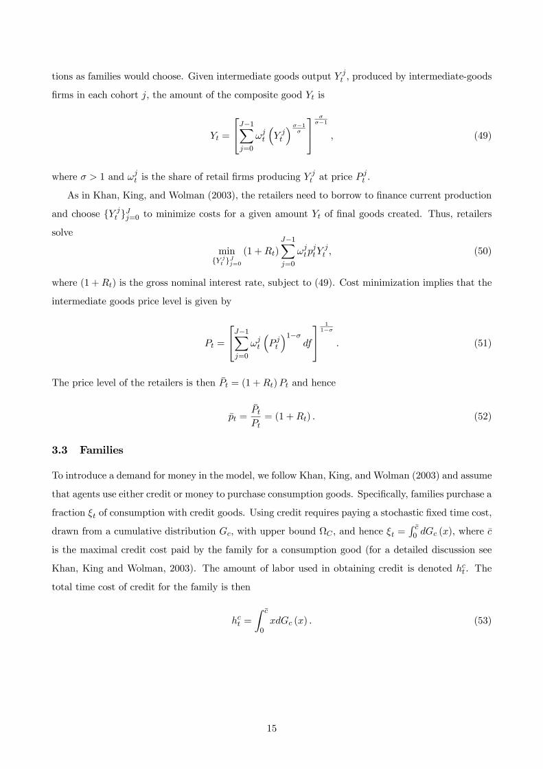
tions as families would choose. Given intermediate goods output , produced by intermediate-goods

firms in each cohort , the amount of the composite good is

=

⎡⎣−1X=0

³

´−1

⎤⎦ −1

(49)

where 1 and is the share of retail firms producing

at price

.

As in Khan, King, and Wolman (2003), the retailers need to borrow to finance current production

and choose =0 to minimize costs for a given amount of final goods created. Thus, retailers

solve

min

=0(1 +)

−1X=0

(50)

where (1 +) is the gross nominal interest rate, subject to (49). Cost minimization implies that the

intermediate goods price level is given by

=

⎡⎣−1X=0

³

´1−

⎤⎦ 11−

(51)

The price level of the retailers is then = (1 +) and hence

=

= (1 +) (52)

3.3 Families

To introduce a demand for money in the model, we follow Khan, King, and Wolman (2003) and assume

that agents use either credit or money to purchase consumption goods. Specifically, families purchase a

fraction of consumption with credit goods. Using credit requires paying a stochastic fixed time cost,

drawn from a cumulative distribution with upper bound Ω , and hence =R 0 (), where

is the maximal credit cost paid by the family for a consumption good (for a detailed discussion see

Khan, King and Wolman, 2003). The amount of labor used in obtaining credit is denoted . The

total time cost of credit for the family is then

=

Z

0

() (53)

15

Families have preferences

∞P=0

−0

⎡⎣ () + −1X=0

¡1− −

¢1−1−

+ (1− ) (1− )

1−

1−

⎤⎦ (54)

where denotes the workers’ hours worked at a wholesale firm, consumption, the number of

employees in wage cohort and aggregate employment. Families hold an aliquot share of all firms.

The budget constraint of the family is given by

+1

1 ++1 ≥ − − +W (55)

where is the price level, is money holdings, bonds, credit debt, consists of lump-sum

transfers from the government and firm dividends, is the one-period nominal interest rate between

period and + 1 and

W =

−1X=0

+ (1− ) (56)

with being the unemployment benefits. Moreover, denotes the workers’ nominal wage in

wage cohort and 1− is equal to the unemployment rate. In real terms

+1

1 ++1 ≥ −

− +

W

(57)

where =

, +1 =

+1

, =

−1 =and =

−1 is the gross inflation rate between

period − 1 and . Since agents purchase a fraction 1 − of consumption goods with money, the

demand for money is

= (1− ) (58)

Similarly, we have that the real credit debt to be paid in period + 1 is +1 = . Using credit

requires paying a stochastic fixed time cost. This cost is realized after the family has decided on the

amount of a product to buy but before choosing between credit or money as the mean of payment.

Here, credit is defined as a one-period interest rate-free loan that needs to be repaid in full the next

period. Families then choose to use credit as long as the gain, , is larger than the cost of credit.17

17That is, the real discounted net gain of placing the transaction amount in a bond for a period and repay the

transaction amount the next period. To see this, combine the first-order condition with respect to (59) together with

the Euler equation (60), below.

16

The family’s first-order conditions with respect to and are, using that = (1 +),

: () = (1 + (1− ))

: =h

¡1− −

¢+ (1− )

(1− )i−1 () (59)

where −1 () is the realization of the credit cost in terms of time.

Using the envelope theorem and the first-order condition with respect to +1 we can write the

family Euler equation as

1 +=

+1

+1 (60)

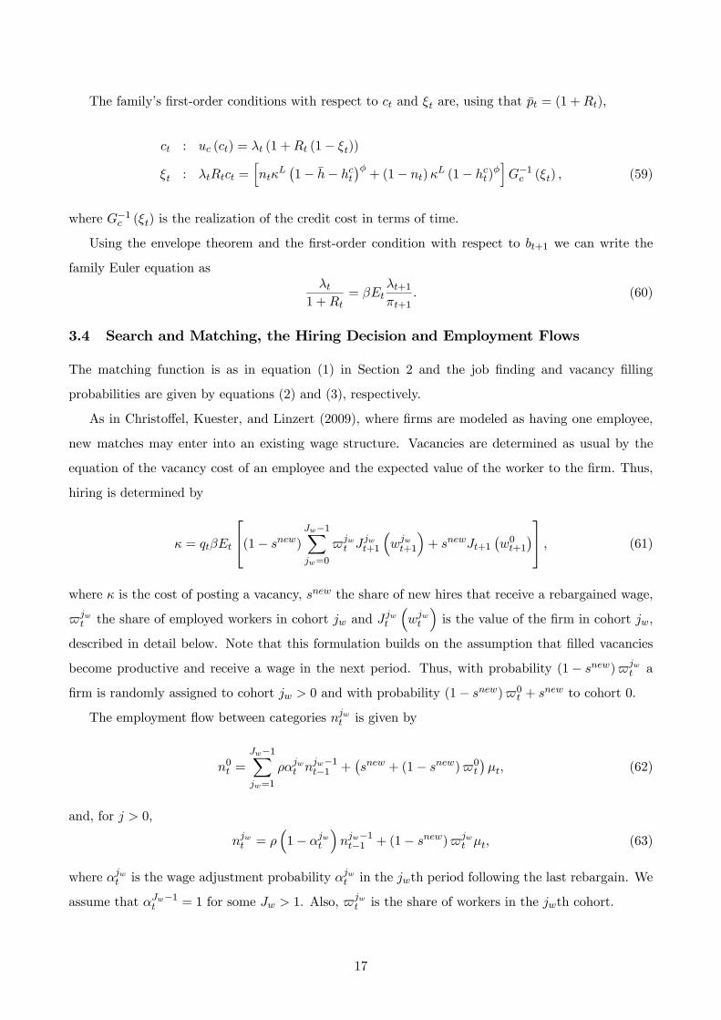
3.4 Search and Matching, the Hiring Decision and Employment Flows

The matching function is as in equation (1) in Section 2 and the job finding and vacancy filling

probabilities are given by equations (2) and (3), respectively.

As in Christoffel, Kuester, and Linzert (2009), where firms are modeled as having one employee,

new matches may enter into an existing wage structure. Vacancies are determined as usual by the

equation of the vacancy cost of an employee and the expected value of the worker to the firm. Thus,

hiring is determined by

=

⎡⎣(1− )

−1X=0

+1

³+1

´+ +1

¡0+1

¢⎤⎦ (61)

where is the cost of posting a vacancy, the share of new hires that receive a rebargained wage,

the share of employed workers in cohort and

³

´is the value of the firm in cohort ,

described in detail below. Note that this formulation builds on the assumption that filled vacancies

become productive and receive a wage in the next period. Thus, with probability (1− ) a

firm is randomly assigned to cohort 0 and with probability (1− )0 + to cohort 0.

The employment flow between categories is given by

0 =

−1X=1

−1−1 +

¡ + (1− )0

¢ (62)

and, for 0,

=

³1−

´−1−1 + (1− )

(63)

where is the wage adjustment probability

in the th period following the last rebargain. We

assume that −1 = 1 for some 1. Also, is the share of workers in the th cohort.

17

Aggregate employment is

=

−1X=0

(64)

and the number of unemployed workers is

= 1− (65)

3.5 Value Functions

The value in period for the family of a worker at a wholesale firm where the wage was last rebargained

in period − is18

³

´=

−

¡1− −

¢1−(1− )

+ Λ+1

³

+1+1 0+1

¡0+1

¢´(66)

+Λ+1

³³1−

+1+1

´+1+1

³+1+1

´+ (1− )+1

´

where is the real wage and

hours worked. The value when being unemployed is

= − (1− )

1−

(1− )+ Λ+1 (+1 + (1− )+1) (67)

where is average value of employment across firms. As in the stylized model above in section 2,

whether newly hired workers get new rebargained wages or enter into a given wage structure of the

firm affects the value of and hence the family’s outside option. We thus have

= 0¡0¢+ (1− )

−1X=0

³

´ (68)

The expected net surplus for the family to have a worker employed in a wholesale firm that last

rebargained wages periods ago is

³

´=

³

´− (69)

18This follows from taking the derivative of the family value in (54) with respect to .

18

and hence, using (66) and (67), the value of an additional employee for the family can then be written

as

³

´=

− −

¡1− −

¢1−(1− )

+ (1− )

1−

(1− )(70)

+Λ+1

h

+1+1 0

+1

¡0+1

¢+

³1−

+1+1

´

+1

³+1+1

´− +1

i

where (= − )) is the net value of getting a job in an average wholesale firm.

The wholesale firm in cohort uses labor as input to produce output, using a constant returns

technology. The value is then

³

´= −

+ Λ+1

+1+1

¡0+1

¡0+1

¢¢(71)

+Λ+1

³1−

+1+1

´

+1+1

³+1+1

´with being a level shifter of productivity.

3.6 Wage Bargaining

To incorporate staggered state-dependent wage bargaining we model wage determination in the spirit

of Haller and Holden (1990) and Holden (1994). However, in order to end up in a wage-setting

formulation that is comparable to standard search and matching models we slightly modify their

set-up. That is, instead of having conflicts as in Haller and Holden (1990) we have a probability of

breakdown.19 The nominal wage 0, when wages are rebargained (i.e., changed), is chosen such that

it solves the Nash product

max 0

¡0

¡0¢¢ ¡

0¡0¢¢1−

(72)

where 0 = 0

and denotes the bargaining power of the family. Otherwise the work continues

according to the old contract as in Holden (1994). The first-order condition with respect to the nominal

wage 0 corresponding to (72) is

0¡0¢0

¡0¢+ (1− )0

¡0¢0

¡0¢= 0 (73)

where the derivatives 0

¡0¢and 0

¡0¢are computed using expressions (70) and (71).

19Specifically, the conflict subgame in Figure 1 in Haller and Holden (1990) is replaced by a subgame where there is a

positive probability of breakdown.

19

The derivative of the family value function is

³

´ 0

1

=

1

+

+1

⎡⎣³1− +1+1

´ +1+1

³+1+1

´ 0

1

+1(74)

−+1+1

0

³

+1+1

³+1+1

´−+1

¡0+1

¢´ 1

+1

#

and the derivative of the value function for the firm is computed similarly.20

3.6.1 Wage Adjustment Probabilities

In the bargaining game, to get a new rebargained wage, one of the parties must find it credible to

threaten with disagreement, which is costly.21 The disagreement costs, drawn at the start of time

period , for the firm, denoted , follows the cumulative distribution function and the cost of

the family follows the cumulative distribution function with upper bounds Ω and Ω , respectively.

The difference in the firm’s value between adjusting the wage or not is

³

´= 0

¡0¢−

³

´ (75)

and similarly for the family

³

´= 0

¡0¢−

³

´ (76)

The firms have incentives to call for rebargaining whenever

³

´and the worker when

³

´. Adjustment probabilities

can then be computed by using (75)-(76) and the

disagreement cost distributions

³

³

´´and

³

³

´´. See Appendix A for a

detailed description of how these objects are computed.

3.7 The Aggregate Resource Constraint and Government Budget Constraint

Total demand is given by

= + (77)

20Note that the derivatives of the value functions are slightly different from those pertaining to price setting; c.f.

equation (46). In price setting the effect of prices on adjustment probabilities are eliminated through the additional

effects on adjustment costs Ξ (which are not present in the value equations (70) and (71)), using an envelope argument.

The effect of wages on adjustment probabilities does not vanish in wage setting because wages are not chosen to maximize

either (70) or (71), but a weighted average of these two; see (73). This implies that the envelope argument used in price

setting is no longer valid. The derivative of the family (firm) value function then has an additional term consisting of

the derivative of the adjustment probabilities.21Note that threats of conflict in wage bargaining will not be exercised along the equilibrium path, but is a credible

threat to enforce a new wage offer. Hence, these costs are not paid in equilibrium, in contrast to costs associated with

price setting.

20

Total supply is From market clearing on the labor market, we have21

−1X=0

=

−1X=0

Ã

!− =

−1X=0

−

−1X=0

Ξ (78)

Combining the expression above with expression (77) and = gives the aggregate resource con-

straint−1X=0

Ã

!−( + ) =

−1X=0

−

−1X=0

Ξ (79)

The government uses lump-sum taxes to finance unemployment benefits. Thus,

= (1− ) (80)

3.8 Optimal Policy

As discussed above, the policy maker needs to take several distortions into account when designing

optimal policy. First, there is imperfect competition in the product market. There is also a distortion

due to money demand and the cost of using credit. Furthermore, there are relative price and wage

distortions. Finally, there are distortions in the hiring decision on the labor market. Here, we focus on

the Ramsey policy as discussed by Schmitt-Grohé and Uribe (2004), maximizing welfare, subject to the

constraints given by optimizing agents in the economy, i.e., for example first-order and market-clearing

conditions.

The policymaker then maximizes (54) subject to the constraints (1) - (3), (40), (42), (44), (45),

(46), (47), (48), (51), the flow equation of prices

=

−1−1

(81)

expressions (59) - (65), (70) - (71), (73) - (74), wage setting adjustment probabilities as described in

the Appendix A, the flow equation of wages

=

−1−1

(82)

and the aggregate resource constraint (79).

21

4 Quantitative Evaluation

4.1 Calibration

For our quantitative evaluation, we assume log preferences in consumption and leisure, i.e., () =

log and = 1. The baseline calibration of the structural parameters is chosen to represent the U.S.

economy on a quarterly basis and is presented in Table 1. We set to 09928 as in Khan, King, and

Table 1: Baseline Calibration of the Model

Parameters

Time preference 09928

Product market substitutability 10

Match-retention rate 09

Family bargaining power 05

Matching function parameter 127

Productivity shifter 5

1− Share of workers entering into existing wage structure 05

Hours worked 02

Disutility of work parameter 24035

Vacancy cost 00486

Income when unemployed 03529

Beta left parameter (prices) 21

Beta right parameter (prices) 1

Ω The largest fixed cost (prices) 00024

= Beta left parameter (wages) 21

= Beta right parameter (wages) 1

Ω = Ω The largest fixed cost (wages) 00396

Beta left parameter (credit) 2806

Beta right parameter (credit) 10446

Ω The largest fixed cost (credit) 00342

Mass of goods with positive credit cost 0361

Wolman (2003). This generates a real interest rate of slightly below 3 percent and is motivated by

data on one-year T-bill rates and the GDP deflator. Note that this is a key parameter for governing

the strength of the monetary distortion.22 For we use a standard value of 10, generating a markup

of around 11 percent. We set the bargaining power = 05, implying symmetrical bargaining in the

baseline calibration. For the job separation rate 1 − , we follow Hall (2005) and set = 09. The

value of is set to 127 following Den Haan, Ramey, and Watson (2000). We set hours worked to 02

and to 5 in order to normalize output per employee to unity.

To calibrate the share of new hires that get rebargained wages, there are several sources of evidence.

Micro-data studies, summarized in Pissarides (2009), seem to indicate that newly hired workers’ wages

are substantially more flexible than incumbents’ wages speaking against the idea that a large share

22For example, using a lower would give the Ramsey planner an incentive to set a lower inflation rate.

22

of entrants enter into an existing wage structure. However, the studies summarized in Pissarides

(2009) generally fail to control for effects stemming from variations in the composition of firms and

match quality over the cycle. Thus, it might be that the empirical evidence just reflects that workers

move from low-wage firms (low-quality matches) to high-wage firms (high-quality matches) in boom

periods and vice versa in recessions. The approach taken to address this issue is to introduce job-

specific fixed effects in a regression of individual wages on the unemployment rate and the interaction

of the unemployment rate and dummy variable indicating if the tenure of the worker is short, see

Gertler and Trigari (2009). This dummy structure controls for composition effects in workers, firms

and match quality. Importantly, the results reported by Gertler and Trigari (2009) no longer indicate

that wages are more sensitive to labor market conditions at the beginning than later in the span of

a match, contrasting Pissarides (2009). This finding is thus in line with a low calibration of .23

Moreover, if we turn to survey evidence, like Bewley (1999), Bewley (2007) for the U.S. and the study

performed within the Eurosystem Wage Dynamics Network (WDN) covering about 15 000 firms in 15

European countries, we see strong evidence that the wages of new hires are tightly linked to those of

incumbents. As reported by Galuscak, Keeney, Nicolitsas, Smets, Strzelecki, and Vodopivec (2012),

about 80% percent of the firms in the WDN survey respond that internal factors (like the internal pay

structure) are more important in driving wages of new hires than market conditions. Taken together

the results points towards a non-neglible share of new hires that enters into an existing wage structure.

However, lacking any sharp evidence on the exact value of this parameter we set to 0.5 in the

baseline calibration and vary the parameter between 0 and 1 in the robustness exercises.

For credit costs, a fraction 1− of the goods costs zero. Then

() =³1−

´+

¡;

Ω

¢ (83)

The cost cumulative distribution functions , , and are beta distributed;

¡;

Ω

¢=

µ

Ω;

¶(84)

for ∈ . Except for Ω and Ω , the parameters for and are calibrated following

Lie (2010) closely.24 For the parameters for the disagreement cost distributions and we set

= = 21 and = = 1 (similar to the values for and taken from Lie, 2010). We also

set Ω = Ω and then choose the parameters , , , Ω , Ω and Ω so that the sticky price and

23As discussed in Gertler and Trigari (2009), additional findings on employment effects of wage contracting presented

in Card (1990) and Olivei and Tenreyro (2007, 2010) provide further evidence in line with a low calibration of .24The reason for this modification of Ω is that other variables enter the money-demand first-order condition (59) in

a slightly different way as compared to Khan, King, and Wolman (2003) and Lie (2010), thus motivating a change so

that inflation under flexible wages is in line with their model.

23

wage model under two percent inflation has vacancy costs of one percent of output, a replacement

rate of 40 percent as in Hall (2005), a matching function elasticity of 06, which is the midpoint of the

interval 05−07 as suggested by Petrongolo and Pissarides (2001), a mean duration of wage contractsof a year as in Taylor (1993), a mean duration of prices of a year in line with Nakamura and Steinsson

(2008) and that the flexible wage model has an optimal policy steady-state deflation rate of 076, as

in Khan, King, and Wolman (2003). The results are presented in Table 1. This calibration implies

that we need to set = 5 and = 8 in order to avoid price/wage setting cohorts without mass.

To solve for the efficient allocation we maximize family welfare, as described in (54), given that

the Friedman rule holds, subject to the matching function (1), the flow equation of employment

= −1 + and the aggregate resource constraint

+ = (85)

4.2 Quantitative Results

To solve for the Ramsey optimal steady-state inflation rate, we follow Schmitt-Grohé and Uribe

(2009).25 In Table 2 we present the Ramsey optimal steady-state inflation rates implied by our model.

In the absence of price or wage rigidities we find, in line with previous literature, that the Ramsey

optimal inflation rate is −285 percent per year. In other words, with no frictions to price or wagesetting, the model replicates the finding of Friedman (1969) that deflation is optimal when there is a

role for money as a medium of exchange.

Table 2: Yearly optimal inflation rate under the Ramsey policy

No Price or Wage Rigidities -2.85

State Dependent Prices only -0.76

State Dependent Prices and Wages 1.15

No monetary frictions (cashless) 1.52

Exogenous adjustment probabilities 2.95

When introducing price rigidities, we see that the Ramsey optimal inflation rate increases, but

remains below zero, as previously pointed out by Khan, King, and Wolman (2003) and Schmitt-

25 The first-order condition in the Ramsey optimal policy consists of the derivatives of the objective with respect to

the control and state variables and derivatives with respect to the Lagrange multipliers for the constraints. Note that

the derivative with respect to the Lagrange multipliers is just the equation system defining the competitive equilibrium

for a given inflation rate. Following along the lines of Schmitt-Grohé and Uribe (2009), we posit an inflation rate 0

and then solve for the competitive equilibrium given the inflation rate. Then a candidate for the Lagrange multiplier

vector is computed using the remaining first-order conditions (i.e. with respect to the control and state variables) as if

these hold, relying on a least-squares method. The candidate Lagrange multiplier is then used to compute the squared

residuals from these first-order conditions. A standard iterative minimization routine can then be used to find the value

of inflation that leads to the sum of squared residuals of these first-order conditions being zero.

24

Grohé and Uribe (2010). In the baseline model, also introducing impediments to continuous wage

rebargaining, the Ramsey optimal inflation rate is 1.15 percent.26 Thus, we see that the Ramsey

optimal inflation rate increases by almost two percentage points in a calibration that implies that

employment is 187 percentage points lower than the efficient allocation.

Removing the monetary friction and looking at the cashless economy as often done in the mone-

tary policy literature, see Woodford (2003), increases inflation to 152 percent. Thus, the monetary

distortion has a moderately negative effect on the optimal policy.

Furthermore, we analyze the importance of endogenous price and wage adjustment probabilities

by fixing the price and wage adjustment probabilities to the values when steady-state inflation is two

percent. Then we solve for the Ramsey policy under these exogenous adjustment probabilities. The

optimal inflation rate increases by slightly less than two percentage points in this case, as compared

to the case with endogenous adjustment probabilities. Thus, the ability of agents to self-select into

adjustment has strong effects on the Ramsey planner’s choice. This result contrasts with Lie (2010),

who finds that endogenizing adjustment probabilities is not important in a model with flexible wages.

To explore the robustness of the results, we next vary the replacement rate. The results from this

exercise can be seen in Table 3. When the replacement rate parameter, , is increased (decreased),

the optimal inflation rate increases (decreases) by 014 (021) percentage points. The intuition is that

an increase in the replacement rate makes the economy less efficient due to an increasing wage as can

be seen from equation (33) in the simple example, thus increasing the net gain for the Ramsey planner

to use inflation to move the economy towards the efficient allocation, as can also be seen in the Hosios

condition (32). Note also that the gross replacement rate, i.e., also taking into account the disutily

of work, is 0952 for the high calibration and 0881 for the low, as compared with 0921 for the

baseline. Thus, the high case pushes the calibration close to the Hagedorn and Manovskii (2008)

calibration.

Varying the share of new hires receiving rebargained wages has big effects. If all new hires get

rebargained wages ( = 1), the wage is, as expected, the same as when wages are flexible, while

when all workers enter into an existing wage structure as in Gertler and Trigari (2009) ( = 0), the

optimal inflation rate is 135 percent.27

Varying the bargaining power has moderate effects on the results; increasing the worker bargaining

power to 06 increases optimal inflation to 127 percent, while reducing it to 04 leads to inflation of

about 097 percent. The reason is that an increase (decrease) in the bargaining power pushes the

26Experimenting with introducing capital accumulation, as in Gertler and Trigari (2009), yields a very similar Ramsey

optimal inflation rate of 0.88 percent.27Note that the share of workers in the first cohort is always larger than , except when = 1, since some of

the workers entering an existing wage structure will enter into the first cohort. In the baseline calibration, the share of

new hires entering into the first cohort and hence getting rebargained wages is 059 while it is 021 when = 0.

25

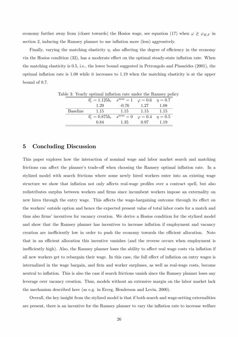
economy further away from (closer towards) the Hosios wage, see equation (17) when ≷ in

section 2, inducing the Ramsey planner to use inflation more (less) aggressively.

Finally, varying the matching elasticity , also affecting the degree of efficiency in the economy

via the Hosios condition (32), has a moderate effect on the optimal steady-state inflation rate. When

the matching elasticity is 05, i.e., the lower bound suggested in Petrongolo and Pissarides (2001), the

optimal inflation rate is 108 while it increases to 119 when the matching elasticity is at the upper

bound of 07.

Table 3: Yearly optimal inflation rate under the Ramsey policy

0 = 1125 = 1 = 06 = 07

1.29 -0.76 1.27 1.08

Baseline 1.15 1.15 1.15 1.15

0 = 0875 = 0 = 04 = 05

0.84 1.35 0.97 1.19

5 Concluding Discussion

This paper explores how the interaction of nominal wage and labor market search and matching

frictions can affect the planner’s trade-off when choosing the Ramsey optimal inflation rate. In a

stylized model with search frictions where some newly hired workers enter into an existing wage

structure we show that inflation not only affects real-wage profiles over a contract spell, but also

redistributes surplus between workers and firms since incumbent workers impose an externality on

new hires through the entry wage. This affects the wage-bargaining outcome through its effect on

the workers’ outside option and hence the expected present value of total labor costs for a match and

thus also firms’ incentives for vacancy creation. We derive a Hosios condition for the stylized model

and show that the Ramsey planner has incentives to increase inflation if employment and vacancy

creation are inefficiently low in order to push the economy towards the efficient allocation. Note

that in an efficient allocation this incentive vanishes (and the reverse occurs when employment is

inefficiently high). Also, the Ramsey planner loses the ability to affect real wage costs via inflation if

all new workers get to rebargain their wage. In this case, the full effect of inflation on entry wages is

internalized in the wage bargain, and firm and worker surpluses, as well as real-wage costs, become

neutral to inflation. This is also the case if search frictions vanish since the Ramsey planner loses any

leverage over vacancy creation. Thus, models without an extensive margin on the labor market lack

the mechanism described here (as e.g. in Erceg, Henderson and Levin, 2000).

Overall, the key insight from the stylized model is that if both search and wage-setting externalities

are present, there is an incentive for the Ramsey planner to vary the inflation rate to increase welfare

26

through its effect on job creation and unemployment.

In the baseline quantitative evaluation, featuring many of the aspects that have been deemed

important in determining the optimal inflation rate, we find that the Ramsey optimal inflation rate

is 115 percent per year. When comparing with a model with flexible wages for new hires, this is an

increase of almost two percentage units, confirming that the mechanism is important in an elaborate

general equilibrium context. Moreover, this result is robust to reasonable variations in the match

elasticity, the workers’ bargaining power, the replacement rate and fairly large variations in the share

of new hires entering into an existing wage structure. When shutting down the monetary distortion

and looking at the cashless economy as is done in a large part of the monetary-policy literature, see

Woodford (2003), we find that the Ramsey optimal inflation rate increases to 152 percent. Thus, the

monetary distortion has a moderately negative effect on the Ramsey planner’s choice.

In conclusion, we show that the combination of nominal wage and search externalities can generate

a Ramsey optimal steady-state inflation rate that is significantly positive and provide a mechanism

that helps reconcile theories of monetary non-neutrality with observed inflation targets of central

banks.

27

References

Adam, K., and R. Billi (2006): “Optimal Monetary Policy under Commitment with a Zero Bound

on Nominal Interest Rates,” Journal of Money, Credit and Banking, 38, 1877—1905.

Amano, R., K. Moran, S. Murchison, and A. Rennison (2009): “Trend inflation, wage and

price rigidities, and productivity growth,” Journal of Monetary Economics, 56, 353 — 364.

Bewley, T. (1999): Why Wages Don’t Fall During a Recession. Harvard University Press, Cam-

bridge, MA.

(2007): “Insights Gained from Conversations with Labor Market Decision Makers,” ECB

Working Paper 776.

Billi, R. (2011): “Optimal Inflation for the US Economy,” American Economic Journal: Macroeco-

nomics, 3, 29—52.

Calvo, G. (1983): “Staggered Prices in a Utility-Maximizing Framework,” Journal of Monetary

Economics, 12, 383—398.

Card, D. (1990): “Unexpected Inflation, Real Wages, and Employment Determination in Union

Contracts,” American Economic Review, 80, 669—88.

Christoffel, K., K. Kuester, and T. Linzert (2009): “The Role of Labor Markets for Euro

Area Monetary Policy,” European Economic Review, 53, 908—936.

Den Haan, W., G. Ramey, and J. Watson (2000): “Job Destruction and Propagation of Shocks,”

American Economic Review, 90, 482—498.

Dotsey, M., R. King, and A. Wolman (1999): “State-Dependent Pricing and the General Equi-

librium Dynamics of Money and Output,” Quarterly Journal of Economics, 114, 655—690.

Erceg, C., D. Henderson, and A. Levin (2000): “Optimal Monetary Policy with Staggered Wage

and Price Contracts,” Journal of Monetary Economics, 46, 281—313.

Faia, E. (2008): “Optimal Monetary Policy Rules with Labor Market Frictions,” Journal of Economic

Dynamics and Control, 32, 1600—1621.

(2009): “Ramsey Monetary Policy with Labor Market Frictions,” Journal of Monetary

Economics, 56, 570—581.

Faia, E., and L. Rossi (2013): “Union Power, Collective Bargaining, And Optimal Monetary Policy,”

Economic Inquiry, 51, 408—427.

Friedman, M. (1969): “The Optimum Quantity of Money,” in The Optimum Quantity of Money,

and Other Essays. Aldine Publishing Company, Chicago, IL.

28

Galuscak, K., M. Keeney, D. Nicolitsas, F. Smets, P. Strzelecki, and M. Vodopivec

(2012): “The Determination of Wages of Newly Hired Employees: Survey Evidence on Internal

Versus External Factors,” Labour Economics, 19, 802—812.

Gertler, M., and A. Trigari (2009): “Unemployment Fluctuations With Staggered Nash Wage

Bargaining,” Journal of Political Economy, 117, 38—86.

Hagedorn, M., and I. Manovskii (2008): “The Cyclical Behavior of Equilibrium Unemployment

and,” American Economic Review, 98, 1692—1706.

Hall, R. (2005): “Employment Fluctuations with EquilibriumWage Stickiness,” American Economic

Review, 95(1), 50—65.

Haller, H., and S. Holden (1990): “A Letter to the Editor on Wage Bargaining,” Journal of

Economic Theory, 52, 232—236.

Holden, S. (1994): “Wage Bargaining and Nominal Rigidities,” European Economic Review, 38,

1021—1039.

Hosios, A. (1990): “On the Efficiency of Matching and Related Models of Search and Unemploy-

ment,” Review of Economic Studies, 57, 279—98.

Khan, A., R. King, and A. Wolman (2003): “Optimal Monetary Policy,” Review of Economic

Studies, 70, 825—860.

Kim, J., and F. Ruge-Murcia (2011): “Monetary Policy when Wages are Downwardly Rigid:

Friedman Meets Tobin,” Journal of Economic Dynamics and Control, 35, 2064—2077.

Lie, D. (2010): “State-Dependent Pricing and Optimal Monetary Policy,” Federal Reserve Bank of

Boston Working Paper 09-22.

Merz, M. (1995): “Search in the Labor Market and the Real Business Cycle Model,” Journal of

Monetary Economics, 36, 269—300.

Mortensen, D., and C. Pissarides (1994): “Job Creation and Job Destruction in the Theory of

Unemployment,” Review of Economic Studies, 61, 397—415.

Nakamura, E., and J. Steinsson (2008): “Five Facts About Prices: A Reevaluation of Menu Cost

Models,” Quarterly Journal of Economics, 123, 1415—1464.

Olivei, G., and S. Tenreyro (2007): “The Timing of Monetary Policy Shocks,” American Eco-

nomic Review, 97, 636—663.

(2010): “Wage-Setting Patterns and Monetary Policy: International Evidence,” Journal of

Monetary Economics, 57, 785—802.

29

Petrongolo, B., and C. Pissarides (2001): “Looking into the Black Box: A Survey of the Match-

ing Function,” Journal of Economic Literature, 39, 390—431.

Pissarides, C. (2000): Equilibrium Unemployment Theory, 2nd Edition. The MIT Press, MA.

(2009): “The Unemployment Volatility Puzzle: Is Wage Stickiness the Answer?,” Economet-

rica, 77(5), 1339—1369.

Ravenna, F., and C. Walsh (2012): “Monetary policy and Labor Market Frictions: A Tax Inter-

pretation,” Journal of Monetary Economics, 59, 180—195.

Rotemberg, J. (1982): “Monopolistic Price Adjustment and Aggregate Output,” Review of Eco-

nomic Studies, 49, 517—531.

Schmitt-Grohé, S., and M. Uribe (2004): “Optimal Fiscal and Monetary Policy under Sticky

Prices,” Journal of Economic Theory, 114, 198—230.

(2009): “Computing Ramsey Equilibria in Medium-Scale Macroeconomic Models,” mimeo.

(2010): “The Optimal Rate of Inflation,” in Handbook of Macroeconomics, ed. by M. Fried-

man, B. M.and Woodford, vol. 3B. Elsevier, San Diego, CA.

(2012a): “Foreign Demand for Domestic Currency and the Optimal Rate of Inflation,”

Journal of Money, Credit, and Banking, 44, 1307—1324.

(2012b): “On Quality Bias and Inflation Targets,” Journal of Monetary Economics, 59,

393—400.

Taylor, J. (1993): “Discretion Versus Policy Rules in Practice,” Carnegie-Rochester Conference

Series on Public Policy, 39, 195—214.

Thomas, C. (2008): “Search and Matching Frictions and Optimal Monetary Policy,” Journal of

Monetary Economics, 55, 936—956.

Trigari, A. (2009): “Equilibrium Unemployment, Job Flows, and Inflation Dynamics,” Journal of

Money, Credit and Banking, 41(1), 1—33.

Woodford, M. (2003): Interest and Prices: Foundations of a Theory of Monetary Policy. Princeton

University Press, Princeton, NJ.

30

Appendix

A Wage Adjustment Probabilities

The fraction of firms that calls a conflict is

1 if Ω

³

´

³

³

´´0 ≤

³

´≤ Ω

0

³

´ 0

(86)

Similarly, the fraction of workers that has an incentive to call a conflict to force a rebargain of the

wage contract is

1 if Ω

³

´

³

³

´´0 ≤

³

´≤ Ω

0

³

´ 0

(87)

The adjustment probabilities are then

=

⎧⎪⎪⎪⎪⎪⎪⎪⎪⎪⎪⎪⎪⎪⎨⎪⎪⎪⎪⎪⎪⎪⎪⎪⎪⎪⎪⎪⎩

1 if Ω

³

´or if Ω

³

´

³

³

´´+

³

³

´´−

³

³

´´

³

³

´´ 0 ≤

³

´≤ Ω

and 0 ≤

³

´≤ Ω

³

³

´´0 ≤

³

´≤ Ω and

³

´ 0

³

³

´´

³

´ 0 and 0 ≤

³

´≤ Ω

0

³

´ 0 and

³

´ 0

(88)

The derivative of the family value function is then, using expressions (70) and (71),

³

´ 0

1

=

1

+

+1

³1−

+1+1

´ +1+1

³+1+1

´ 0

1

+1(89)

−

⎡⎣⎛⎝ +1+1

³

´ +1+1

³+1+1

´ 0

1

+1+

+1+1

³

´ +1+1

³+1+1

´ 0

1

+1

⎞⎠×+1

³

+1+1

³+1+1

´−0

+1

¡0+1

¢´¸

31

Multiplying by 0 gives

³

´ 0

0 1

=

0

+ +1

³1−

+1+1

´ +1+1

³+1+1

´ 0

0

+1(90)

−

⎡⎣⎛⎝ +1+1

³

´ +1+1

³+1+1

´ 0

0

+1+

+1+1

³

´ +1+1

³+1+1

´ 0

0

+1

⎞⎠×+1

³

+1+1

³+1+1

´−0

+1

¡0+1

¢´i

32