1

Introduction to Labview ECE 198 Lab Manual

Introduction

Labview is a versatile graphical programming language which, because of its relatively

simple user interface, should allow you, the programmer, to be writing functional

programs in no time.

This booklet will serve as an introduction to the programming language of Labview and

will introduce you to the most important aspects of the programming language, focusing

on those parts of Labview you will need to successfully complete the labs for ECE

198DW. In particular, Labview is ideally suited for controlling various hardware devices

and recording data. If you recall, we used a Labview program to take data from our

home-made spectrometer setup during the second lab.

Before we dive in, however, we should understand why we are using Labview and what

the advantages and limitations of the program are. Labview is extremely easy to use and,

for relatively small programs, easy to debug. All of the programming is done graphically

with icons and does not require any sort of complicated syntax. If you can use a mouse,

you can program in Labview.

Note that compared to other programming languages, the graphical representation of

Labview uses more memory: this reduces the speed of your programs. This is especially

true for earlier versions of Labview, though the program has improved in later editions.

For our purposes, speed will not be a major concern, so a program like Labview is an

ideal introduction to programming.

This manual will walk you through the basics of the Labview programming language. In

this course, we will only scratch the surface of Labview’s powerful and extensive

capabilities.

The Labview tutorial will consist of the following:

I) Getting Started

II) Basic Mathematical Functions

III) “For” Loops, Sequences, and Plotting

IV) Boolean Operators, Rings, and Case Structures

V) Working with Data Files

VI) Troubleshooting

Labview is installed on all the computers in the lab, and is available from the CITES

webstore.

2

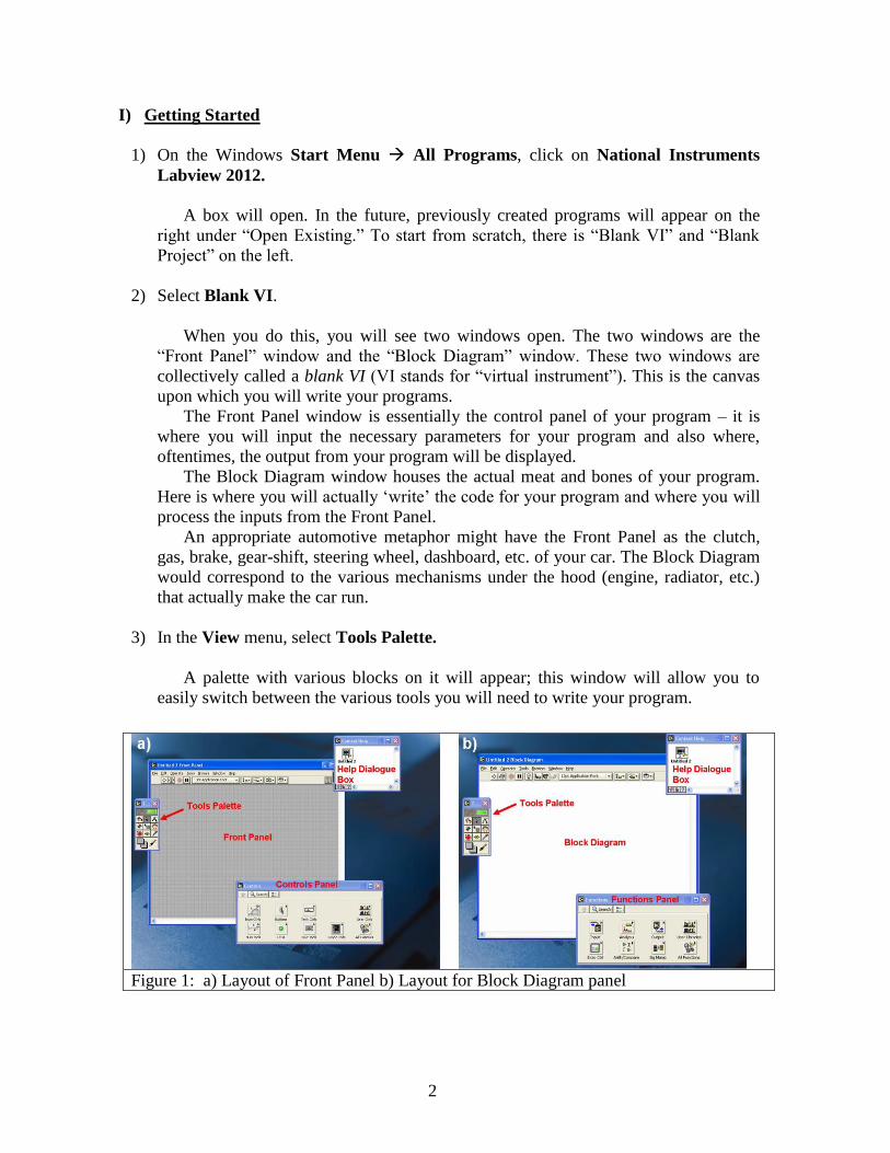
I) Getting Started

1) On the Windows Start Menu All Programs, click on National Instruments

Labview 2012.

A box will open. In the future, previously created programs will appear on the

right under “Open Existing.” To start from scratch, there is “Blank VI” and “Blank

Project” on the left.

2) Select Blank VI.

When you do this, you will see two windows open. The two windows are the

“Front Panel” window and the “Block Diagram” window. These two windows are

collectively called a blank VI (VI stands for “virtual instrument”). This is the canvas

upon which you will write your programs.

The Front Panel window is essentially the control panel of your program – it is

where you will input the necessary parameters for your program and also where,

oftentimes, the output from your program will be displayed.

The Block Diagram window houses the actual meat and bones of your program.

Here is where you will actually ‘write’ the code for your program and where you will

process the inputs from the Front Panel.

An appropriate automotive metaphor might have the Front Panel as the clutch,

gas, brake, gear-shift, steering wheel, dashboard, etc. of your car. The Block Diagram

would correspond to the various mechanisms under the hood (engine, radiator, etc.)

that actually make the car run.

3) In the View menu, select Tools Palette.

A palette with various blocks on it will appear; this window will allow you to

easily switch between the various tools you will need to write your program.

Figure 1: a) Layout of Front Panel b) Layout for Block Diagram panel

3

When you select the Front Panel, you will also see a window labeled Controls. (If

you do not see it, open it by going to View Controls Palette.) This window is

your Controls palette, which will provide you with all the building blocks necessary

to construct your Front Panel.

Likewise, when you select the Block Diagram, you should see a Functions palette

(View Functions Palette). This is the Block Diagram equivalent of the Front

Panel Controls palette and provides all the tools necessary for building your program

in the Block Diagram window.

Finally, you should also see a Help window on the screen (Help Show

Context Help). As you move your mouse over the various objects in your Front

Panel or Block Diagram, this window will provide you with information about how it

works.

4

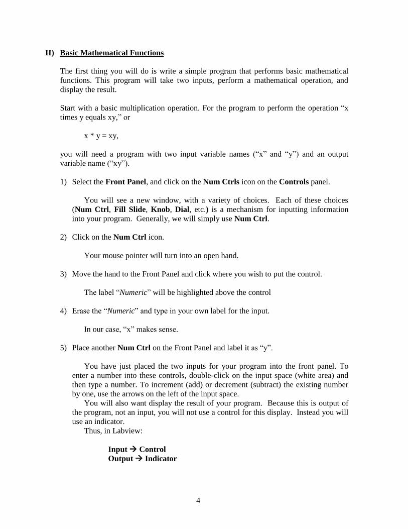
II) Basic Mathematical Functions

The first thing you will do is write a simple program that performs basic mathematical

functions. This program will take two inputs, perform a mathematical operation, and

display the result.

Start with a basic multiplication operation. For the program to perform the operation “x

times y equals xy,” or

x * y = xy,

you will need a program with two input variable names (“x” and “y”) and an output

variable name (“xy”).

1) Select the Front Panel, and click on the Num Ctrls icon on the Controls panel.

You will see a new window, with a variety of choices. Each of these choices

(Num Ctrl, Fill Slide, Knob, Dial, etc.) is a mechanism for inputting information

into your program. Generally, we will simply use Num Ctrl.

2) Click on the Num Ctrl icon.

Your mouse pointer will turn into an open hand.

3) Move the hand to the Front Panel and click where you wish to put the control.

The label “Numeric” will be highlighted above the control

4) Erase the “Numeric” and type in your own label for the input.

In our case, “x” makes sense.

5) Place another Num Ctrl on the Front Panel and label it as “y”.

You have just placed the two inputs for your program into the front panel. To

enter a number into these controls, double-click on the input space (white area) and

then type a number. To increment (add) or decrement (subtract) the existing number

by one, use the arrows on the left of the input space.

You will also want display the result of your program. Because this is output of

the program, not an input, you will not use a control for this display. Instead you will

use an indicator.

Thus, in Labview:

Input Control

Output Indicator

5

Because you are now in the Numeric Controls menu of the Controls panel, hit

the “Express” label to get back to the higher level menu. Note: The express menu

contains the most commonly used Labview tools. To get access to the full selection,

press the double arrow button at the bottom of the Controls palette.

6) Select Num Inds.

Again, you will have the option of choosing a variety of indicators.

7) Choose the Num Ind icon, place it on the front panel, and label it “xy”.

We are now ready to go to the block diagram. Before we do, make sure your

screen looks something like that shown in Figure 2.

When you go back to the Block Diagram, you should see three rectangles labeled

“x”, “y”, and “xy”. These are the graphical representations of the controls and

indicators you have just created.

You will notice that the controls have a filled orange border which shows that

they are controls and meant to be read by your program. The indicator has an unfilled

orange border, labeling it as an indicator and demonstrating that it is meant to be

written to instead of read from.

8) In the Functions palette, click on the Arith & Compare icon, and then the Numeric

icon.

The Numeric window should show you a number of arithmetic operators.

9) Choose the Multiply operator, and place it on your Block Diagram window.

Figure 2: Front Panel after controls “x” and “y” and indicator “xy” have been created.

Controls Panel was left in the “Numeric Controls” window. To return to the “Controls”

menu, simply click on the “up” arrow in the upper left hand side of the dialogue box.

6

You now have everything in place to write your program. All that is left is to wire

it up.

You will notice that when you put the mouse over the multiply operator, three

leads appear, looking like dots with wires protruding slightly from them. These leads

are identified in the Context Help window. For more complicated icons, the Context

Help window not only labels the leads, but describes their purpose and the required

input.

As you can see from the Context Help window, the two leads on the left are for

your inputs while the lead on the right is for your output. When you place the mouse

cursor over the leads, it will turn into a spool of wire. Clicking on the lead while the

pointer is in this form will attach a wire to that lead.

10) Attach a wire to the ‘x” lead on the multiply operator, then move your mouse to the

“x” rectangle and click.

When a wire can be correctly attached to a control or an indicator, a blinking

output lead will appear on the right/left side of that control/indicator.

You have now connected the “x” input to the multiply operator.

11) Now do the same for the “y” lead and “y” rectangle, but click the mouse a couple of

times on the Block Diagram “canvas” between the “y” lead and the y rectangle.

You can pin the wire to locations on your block diagram by doing this. This can

be helpful for maneuvering wires through more complicated block diagrams.

12) Attach a wire between the “xy” rectangle and the output of the Multiply operator.

Once you have connected the output lead of the multiply operator to the xy

rectangle, you have finished “writing” your program.

13) Go back to the Front Panel and enter numbers into the “x” and “y” inputs.

On the upper left hand corner of the front Panel there is a white arrow. This is the

run arrow. Clicking the arrow will run your program

If the arrow icon appears broken, there is something wrong with your program.

Look for loose wires or misconnected icons.

When the arrow is white, your program will run. Note: a program that is capable

of running is in no way a guarantee that it will correctly do what you want it to do!

.

14) Click run.

Congratulations! You have just run your first Labview program!

15) Go to File Save and save your program as “yournamemath”.

7

This saves your program as a “*.vi” file, which is the Labview format for

programs.

Try playing around with your program. Add inputs and/or add operations. Make the math

more complex. Familiarize yourself with the numeric operators including the more

complicated trigonometric and logarithmic functions.

8

III) Loops, Sequences, and Plotting

Now that we have mastered the basic set-up for a Labview *.vi program/file, let’s try to

write a slightly more complicated program. For this program, you will create a set of

numbers, or an array of numbers, and then plot these numbers onto a XY-graph.

1) Open up a new *.vi (File New VI, or Ctrl + N)

For starters, we will try to create an array consisting of two columns. The first

will be the ‘x’ column. The second will be the ‘y’ column, where ‘y’ will be a

function of ‘x’. To begin, let’s use the function y = sin(x).

In order to create a graph of y vs. x, you will first need to decide what range of x

values you are interested in. For instance, you might want to look at 0 < x < 3.14, at

x-intervals of 0.01. In order to determine your range and resolution, you will need to

create three controls: the starting point (xstart), the end point (xend), and the

resolution (xres). On the Block Diagram window, you should see the variables xstart,

xend, and xres displayed.

Because this will be a slightly more complicated *.vi than the yournamemath.vi

program in II), we will need to build a sequence. The sequence function is simply a

mechanism for chronologically ordering the operations you wish to perform in your

program. When Labview encounters a sequence it performs all of the operations

programmed into the first frame, “Frame 0”, then moves to the next (“Frame 1”), and

the next until it reaches the last frame of the sequence, at which point it moves on to

the remaining operation in the program.

1) Go to the Functions window (if you don’t see it, just right click the mouse and it

should appear), click Exec Ctrl, and select Flat Sequence.

2) Drag your mouse cursor across your Block Diagram window to create a rectangle (it

should look like a strip of film).

This is your Sequence.

3) Right-click on the edge of the Sequence and select Replace with Stacked Sequence.

There are two types of Sequences, the “flat” and the “stacked” sequence. From a

programming point of view, they are identical. The only difference between the two

is the way they are depicted in the Block Diagram window. A Stacked Sequence

shows only one frame at a time, while a Flat Sequence shows all of the frames at the

same time, like a film strip. I find that the Stacked Sequence is easier to use in a

program since it takes up less space, however, many of the freeze screens in this

manual use Flat Sequences, so that you can see the entire sequence in one screen.

4) Right-click on the edge of the Stacked Sequence (which looks exactly the same) and

select Add Frame After.

9

You should see a label on the top of the frame appear: “1[0..1]”.

This tells you that you are looking at frame 1 of the two frames in your sequence

(frames 0 and 1). To move between frames, click the left and right arrows on either

side of this label to move between frames.

When the computer runs your program, it will perform all the requested

operations in Frame 0, and then move on and do the same for Frame 1.

Before we start programming, we will need to make a somewhat lengthy digression

which will acquaint you with quite a few concepts that you will need to proceed.

A variable in Labview is represented by the rectangle in the Block Diagram window that

is created when you place a control or indicator (or Boolean or String, for that matter) on

the Front Panel screen. When you create a variable in Labview you may also want to use

that variable at more than one place in your program. In the previous program, we simply

wired the operator directly to the variable. You can imagine that in a complicated

program where each variable is used many times it could become quite messy to have

many wires all going to the same variable.

The solution is called a “local variable”. Local variables are little boxes labeled with the

variable’s name which can be used in place of the actual variable throughout your

program. We will never wire directly to our variables. Instead, we will always use local

variables.

To create a local variable:

i) Right-click on the original variable

ii) Go to Create Local Variable.

The Local Variable that is created is automatically designed to be written

to. When that operation is performed, the value local variable (and thus the

original variable) is changed.

If you instead want to read information from the local variable, simply

right-click on the local variable and select Change to Read.

When you defined your resolution (“xres”), your starting point (“xstart”), and your end

point (“xend”), you also implicitly defined the number of data points you will be plotting.

Figure out the equation that will give you the number of data points: it only requires a

little math to figure out. You will need this value for the program you are writing. Your

program should use “xstart”, “xend” and “xres” to determine the value for “xsteps”.

5) Create local variables of each of the three controls “xstart”, “xend”, and “xres”.

Change them to read (see above), and then place them inside the sequence.

10

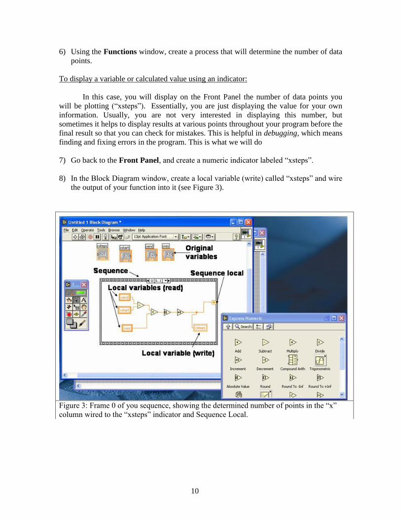
6) Using the Functions window, create a process that will determine the number of data

points.

To display a variable or calculated value using an indicator:

In this case, you will display on the Front Panel the number of data points you

will be plotting (“xsteps”). Essentially, you are just displaying the value for your own

information. Usually, you are not very interested in displaying this number, but

sometimes it helps to display results at various points throughout your program before the

final result so that you can check for mistakes. This is helpful in debugging, which means

finding and fixing errors in the program. This is what we will do

7) Go back to the Front Panel, and create a numeric indicator labeled “xsteps”.

8) In the Block Diagram window, create a local variable (write) called “xsteps” and wire

the output of your function into it (see Figure 3).

Figure 3: Frame 0 of you sequence, showing the determined number of points in the “x”

column wired to the “xsteps” indicator and Sequence Local.

11

Alternatively, one could eschew the use of an indicator variable to store the value

and instead wire to the function output directly. This is a little tricky because the number

will not be used again in this frame of the sequence. Thus, we need to be able to have a

way to take the value of “xsteps” from this frame to subsequent frames. To do this, we

will use a device called a Sequence Local.

To access a value directly:

9) Right-click on the side of the sequence and select Add Sequence Local.

A yellow box will appear on the side of the sequence.

10) Wire the output corresponding to “xsteps” to this box.

A similar box will appear in the same place on all of the other frames in the

program, simply wire to those boxes to access your number in those frames. For the

purposes of this tutorial, I will use both the Sequence Local and the Numeric

Indicator in my wiring (see Figure 3).

To build a For Loop:

11) Go to the Functions window and select Programming (expand the Functions

palatte selection choices). Select Structures, and then For Loop.

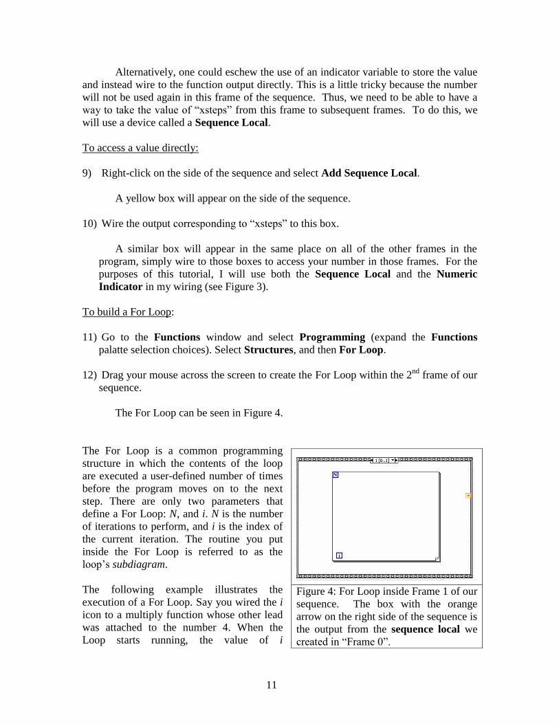
12) Drag your mouse across the screen to create the For Loop within the 2nd

frame of our

sequence.

The For Loop can be seen in Figure 4.

The For Loop is a common programming

structure in which the contents of the loop

are executed a user-defined number of times

before the program moves on to the next

step. There are only two parameters that

define a For Loop: N, and i. N is the number

of iterations to perform, and i is the index of

the current iteration. The routine you put

inside the For Loop is referred to as the

loop’s subdiagram.

The following example illustrates the

execution of a For Loop. Say you wired the i

icon to a multiply function whose other lead

was attached to the number 4. When the

Loop starts running, the value of i

Figure 4: For Loop inside Frame 1 of our

sequence. The box with the orange

arrow on the right side of the sequence is

the output from the sequence local we

created in “Frame 0”.

12

automatically starts set to 0. In its first iteration, the For Loop will calculate 0 * 4 = 0.

The program will then loop back and perform the calculation again, except that this time

using i = 1. The result of the subdiagram’s calculation for this iteration will then be 1 * 4

= 4. The For Loop will continue to do this, looping back and incrementing i by 1. The

Loop will perform “N” loops, where N is determined by the programmer.

Oftentimes, you will want to take some information you created in the nth

iteration

of the For Loop and use it in the nth

+1 iteration. To pass information between iterations,

you can use a shift register. A shift register is similar to the Sequence Local that we

learned about earlier. To create a shift register, right-click on the side of the For Loop

and select Add Shift Register.

13) Add a Shift Register to your For Loop.

14) Wire the appropriate number (“xsteps”) to N

This can be done either by using the sequence local you created in Frame 0 or by

creating a local (read) variable for “xsteps” and wiring it to N. N is always wired from

the outside of the For Loop. Now the For Loop will execute “xsteps” number of

loops; one for every point data point.

Our next task will be to create a function which generates, in the form of a 1-D array, the

x-points we wish to plot.

We know our first point in the 1-D array should be x = “xstart”; our second point in the

array should be “xstart” + ”xres”; then “xstart” + “xres” * 2 and so on. Hence, for the ith

point we can say that:

x(i) = xstart + xres * i

15) Program this equation in the subdiagram.

The tricky part is to build an array which will hold our x-points. The first thing we

need to do, before we start running our loop, is to create and initialize (set to zero) an

array. It is important to initialize the array because Labview will store the array you

create in its memory. Without initializing, if you run the program twice in a row it will

just add to the first array it created instead of creating a separate array. If you initialize

the array each time you run the program, this won’t happen.

13

To initialize an array:

16) Go to Functions Programming Arrays Initialize Array.

Place the Initialize Array icon just outside of the For Loop, but inside Frame 1 of

the sequence.

17) To initialize the array, wire the value “0” to both of the inputs on the lower left hand

side of the Initialize Array icon.

In order to wire “0”, you will need to create what is known as a numerical

constant, and set it to “0”. To create a number, go to Functions Programming

Numeric Numeric Constant and place the number, or numeric constant, on your

block diagram. Wire the number into both the “dimension size” and “element” input

leads.

This creates a 0x0 array with all elements set to zero.

18) Wire the output of the Initialize Array icon into the Left Shift Register (the yellow

downward-facing arrow on the left edge of the For Loop).

What this does is tell the For Loop that the array you are building begins as an

initialized, 0x0 array.

19) Next, go to Functions Programming Array Build Array and place this

icon in your For Loop.

20) Right click on the Build Array icon and select Add Input.

Your Build Array icon should now have three leads, two input and one output.

21) Wire the Left Shift Register to the upper left lead of the build array operator, your

value for x(i) (located in the For Loop) into the lower left lead, and wire the Right

Shift Register to the right lead.

Your For Loop will now automatically build your x-array.

How a For Loop builds an array:

i) Before the For Loop starts, the array is initialized to 0 and sent to the

Build Array icon. A number is also wired to “N”, telling Labview how

many iterations to perform. Once this is done, nothing outside of the For

Loop will affect the calculations you perform inside the Loop.

14

ii) At the Build Array step/icon, the output x(0) [ i.e. the function x(i) when

i=0] is added to the array.

Since we initialized the array to have zero elements, this is the first

element of the array (index 0).

iii) The array, now with a length of one, is sent to the right shift register.

iv) The For Loop now moves on to i = 1.

The value kept in the Right Shift Register shifts to the Left Shift

Register for the next iteration.

v) For i = 1, the array, now in the left shift register, is transferred to the Build

Array icon, where x(1) [ i.e. x( i = 1 ) ], is added to the array.

The new array is sent to the Right Shift Register. Now the array is

two elements, x( i = 0 ) and x( i = 1 ), so that

array = [x( i = 0 ), x( i = 1 )]

vi) Steps iii), iv), and v) are repeated, with i incremented each time, until i

reaches N-1.

In the end, your For Loop should have done N number of loops, after

which your array should be:

array = [x( i = 0 ), x( i = 1 ), …, x( i = N-2 ), x( i = N-1 )]

The last step which we need to do in creating our array is, once the For Loop stops

running, to store the array we have created. To do this we need to create an Array

Variable.

22) In the Front Panel, go to the Controls palette, select Controls Modern Array,

Matrix & Cluster Array.

This creates an Array Variable.

23) Name your Array Variable “XArray”.

However, we still have to tell Labview what kinds of variables this is array holds.

You can have arrays of many different types variables. Labview can deal with arrays

of numbers, strings (letters), or even arrays of other arrays. The only requirement is

that the array elements must all be of the same data type (strings, numbers, filenames,

etc..)

15

14) Select Controls Express Num Inds Num Ind, and place the Numeric

Indicator variable inside the open space of the “XArray” variable.

You have now created a numeric array variable.

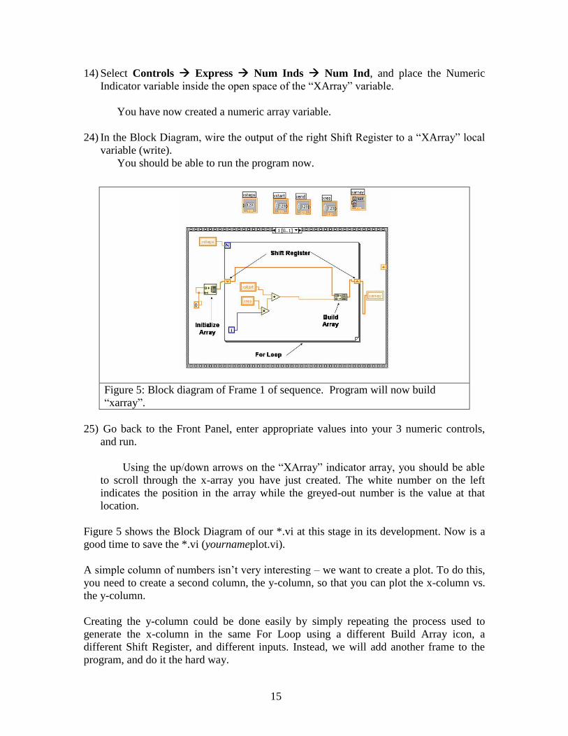
24) In the Block Diagram, wire the output of the right Shift Register to a “XArray” local

variable (write).

You should be able to run the program now.

25) Go back to the Front Panel, enter appropriate values into your 3 numeric controls,

and run.

Using the up/down arrows on the “XArray” indicator array, you should be able

to scroll through the x-array you have just created. The white number on the left

indicates the position in the array while the greyed-out number is the value at that

location.

Figure 5 shows the Block Diagram of our *.vi at this stage in its development. Now is a

good time to save the *.vi (yournameplot.vi).

A simple column of numbers isn’t very interesting – we want to create a plot. To do this,

you need to create a second column, the y-column, so that you can plot the x-column vs.

the y-column.

Creating the y-column could be done easily by simply repeating the process used to

generate the x-column in the same For Loop using a different Build Array icon, a

different Shift Register, and different inputs. Instead, we will add another frame to the

program, and do it the hard way.

Figure 5: Block diagram of Frame 1 of sequence. Program will now build

“xarray”.

16

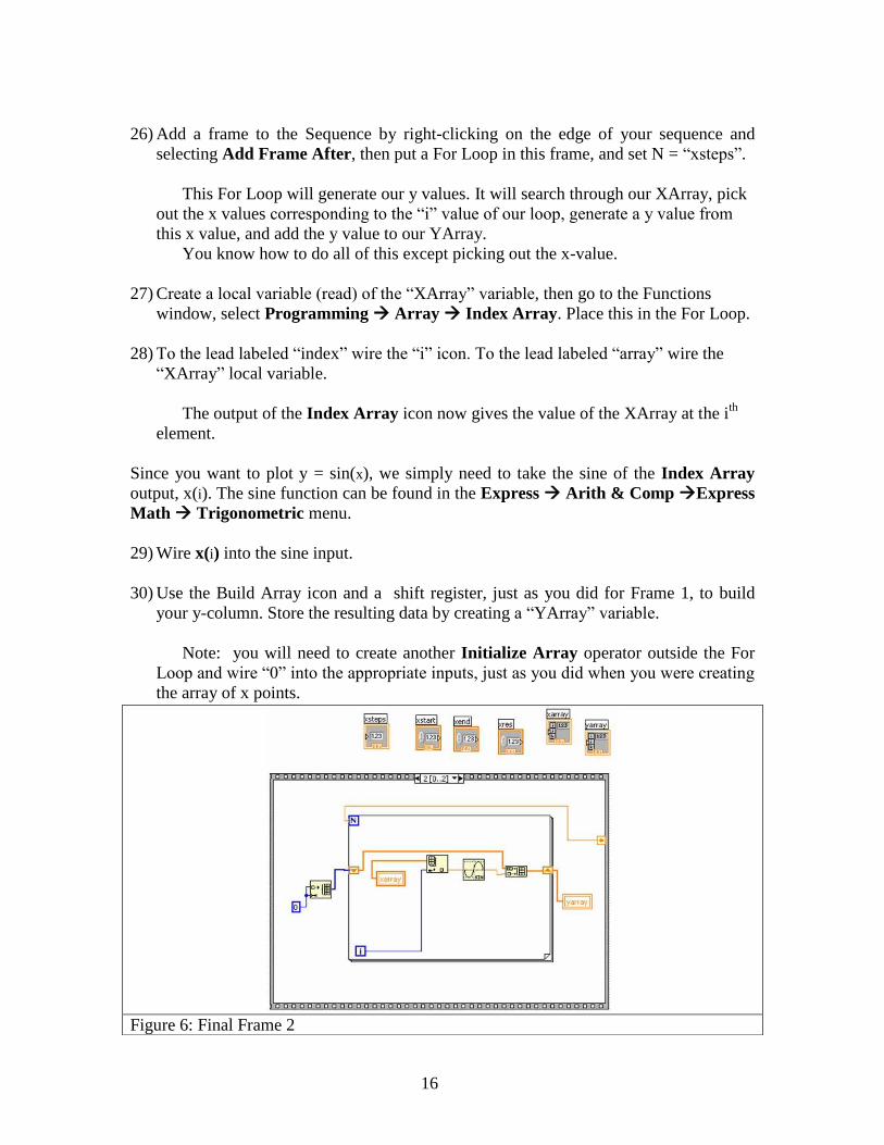
26) Add a frame to the Sequence by right-clicking on the edge of your sequence and

selecting Add Frame After, then put a For Loop in this frame, and set N = “xsteps”.

This For Loop will generate our y values. It will search through our XArray, pick

out the x values corresponding to the “i” value of our loop, generate a y value from

this x value, and add the y value to our YArray.

You know how to do all of this except picking out the x-value.

27) Create a local variable (read) of the “XArray” variable, then go to the Functions

window, select Programming Array Index Array. Place this in the For Loop.

28) To the lead labeled “index” wire the “i” icon. To the lead labeled “array” wire the

“XArray” local variable.

The output of the Index Array icon now gives the value of the XArray at the ith

element.

Since you want to plot y = sin(x), we simply need to take the sine of the Index Array

output, x(i). The sine function can be found in the Express Arith & Comp Express

Math Trigonometric menu.

29) Wire x(i) into the sine input.

30) Use the Build Array icon and a shift register, just as you did for Frame 1, to build

your y-column. Store the resulting data by creating a “YArray” variable.

Note: you will need to create another Initialize Array operator outside the For

Loop and wire “0” into the appropriate inputs, just as you did when you were creating

the array of x points.

Figure 6: Final Frame 2

17

Now you are ready to plot the data.

31) On the Front Panel, select Express Graph Inds XY Graph. Place the (rather

large) icon on your front panel.

32) Go back to the Block Diagram window, add a frame to the sequence, and place the

entire XYGraph icon into this new frame (Frame 3).

33) Create local variables (read) for XArray and YArray.

Note that the XY Graph icon has one input despite requiring multiple arrays of

data. To provide the appropriate input, we must bundle XArray and YArray to

form one datapath.

34) Select Programming Cluster, Class & Variant Bundle, add it to the Block

Diagram, wire appropriately.

35) Run your program.

You should see a sine wave generated on the XY plot on the Front Panel.

36) Save your *.vi (yournameplot.vi)

37) Go to Save As and save the same file as yournameplot2.vi.

18

IV) Boolean Operators, Rings, and Case Structures

Using the *.vi you wrote in the previous tutorial, we will now introduce the concepts of

Boolean operators, case structures, and rings.

The first adjustment we will make to the program will allow the user to choose from a

variety of functions to plot. Think of 5 functions you want to plot where y = f(x). For

notational purposes, these will now be referred to as f1(x), f2(x), f3(x), etc.

1) Delete the Sine icon in Frame 2 of your program.

2) In that For Loop, insert a Case Structure (Programming Structures Case

Structure).

The case structure is a pretty simple concept. At its most basic, the case

structure’s main input is a Boolean, either a “true” or a “false”. Depending on the

value of the input Boolean, the case structure will perform different operations.

When you created a case structure, the default is a true/false case structure,

meaning there is a selector with a value of either true or false. Depending on the value

of the selector, a different process is performed. Figure 7 shows two different cases

for a true/false case structure.

You can change the case structure to be conditional on something other than a

Boolean, but the idea remains the same. The case structure will perform only the

actions set out in the case that is selected.

Figure 7: Examples of True/False Case structures. a) The input here is “True”, so the

operation “xend” x “xstart” is performed and output from the structure. In b), the input is

“False”, so the operation “xstart” – “xend” is performed and output. Note: The

operations here are arbitrary and don’t relate to our current program.

3) Go back to the Front Panel. In the Controls palette, select Express Text Ctrls

Menu Ring and label the Menu Ring “f(x)” after you’ve placed it on the Front Panel.

The menu ring will allow the user of your program to choose the desired function

they wish to plot.

19

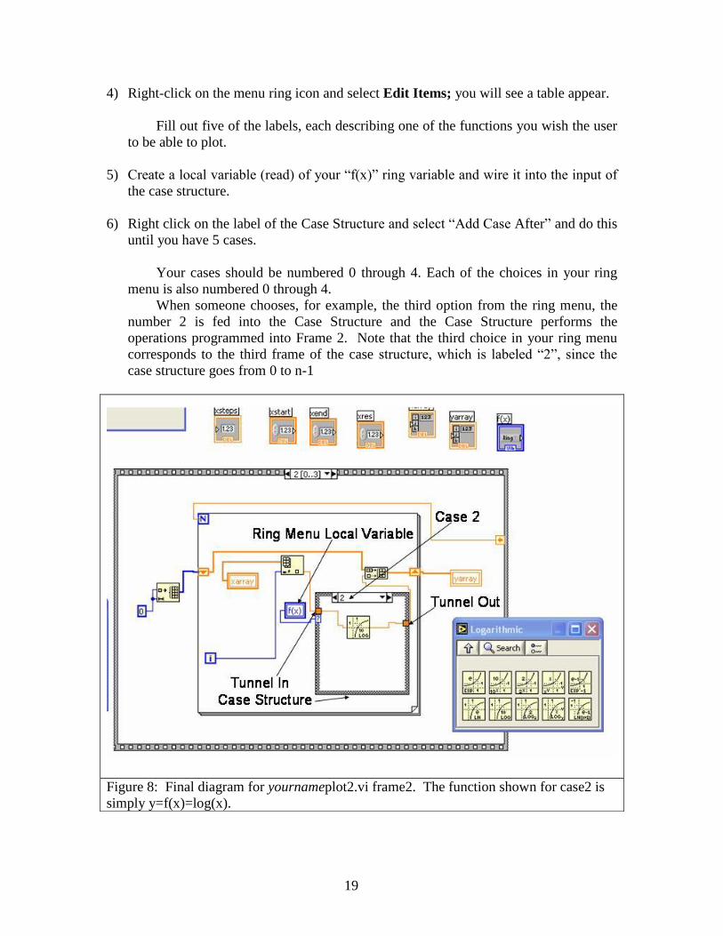
4) Right-click on the menu ring icon and select Edit Items; you will see a table appear.

Fill out five of the labels, each describing one of the functions you wish the user

to be able to plot.

5) Create a local variable (read) of your “f(x)” ring variable and wire it into the input of

the case structure.

6) Right click on the label of the Case Structure and select “Add Case After” and do this

until you have 5 cases.

Your cases should be numbered 0 through 4. Each of the choices in your ring

menu is also numbered 0 through 4.

When someone chooses, for example, the third option from the ring menu, the

number 2 is fed into the Case Structure and the Case Structure performs the

operations programmed into Frame 2. Note that the third choice in your ring menu

corresponds to the third frame of the case structure, which is labeled “2”, since the

case structure goes from 0 to n-1

Figure 8: Final diagram for yournameplot2.vi frame2. The function shown for case2 is

simply y=f(x)=log(x).

20

7) Wire x(i) to the left side of the Case Structure, and wire the right side of the Case

Structure to the Build Array icon.

Where each of these wires attaches to the Case Structure, you should see a yellow

rectangle. This is a “tunnel” to get data in and out of the structure.

For each case in the structure, you must have something connected to each of the

tunnels. If you do not wish to perform an operation on x(i) for a given case, just

connect the two tunnels with a wire.

8) Fill in each of the case structures with one of your desired functions f(x). Use the

x(i) tunnel as your “x”, and wire the output to the output tunnel.

9) Now run the program.

Make sure each case you select from the menu ring gives you the correct plot on

your graph.

10) Save this program as yournameplot2.vi.

21

V) Working with Data Files

At some point in these labs, you will want to read data from a text file or write data to a

text file. Labview makes these operations relatively simple.

1) Open up yournameplot2.vi and save it as “yournamereadwrite1.vi”.

2) In the Block Diagram window, create a new frame between the current Frame 2 and

Frame 3, using either Add Frame After or Add Frame Before.

In this frame you will write the data you have created to a file.

3) In the Programming window, select File I/O, and then Write to Spreadsheet File.

Place the Write to Spreadsheet File icon in the new, blank Frame 3.

When Labview performs any operation on a file, it needs to be told the file name

and location. This is done through the File Path tab on the Write to Spreadsheet File

icon. If you leave this tab blank, a dialogue box will pop up when you run your

program, and you will have to choose the file name and location. This is fine for the

first time you access (or create) a file, but if you write to or read from the file many

times during a program, you do not want to have to manually select the file each time.

To avoid this, you can have Labview remember the file you have created/selected

as a variable in your program. These variables are slightly different than the ones you

have been using thus far as they are “pathname” variables, not “numeric” variables.

4) Leave the File Path tab open, and place new local variables for the “XArray” and

“YArray” variables in Frame 3.

You will need to wire the desired data into one of the data input tabs. Because we

are interested in storing two arrays (x and y), we will want to wire our data into the

2D Data tab. In order to write both as columns, we will need to combine the arrays.

5) Use the Programming Array Build Array icon, and add an input by right-

clicking on the icon.

6) Wire your XArray local variable into the top input, the YArray variable into the

bottom, and wire the Build Array icon output to the 2D Data input of the Write to

Spreadsheet File icon.

Because you want to create this data file from scratch, you can leave the Add to File tab

unwired. The default setting is a False, meaning a new file.

However, you will need to wire a true constant icon to the Transpose tab. This is because

Labview will automatically try to write our data as rows unless we tell it to do otherwise.

When you finish this program, try looking at the difference in your files depending on

whether the Transpose tab is wired to a true or false constant. The true/false constants

can be found in the Programming Boolean window.

22

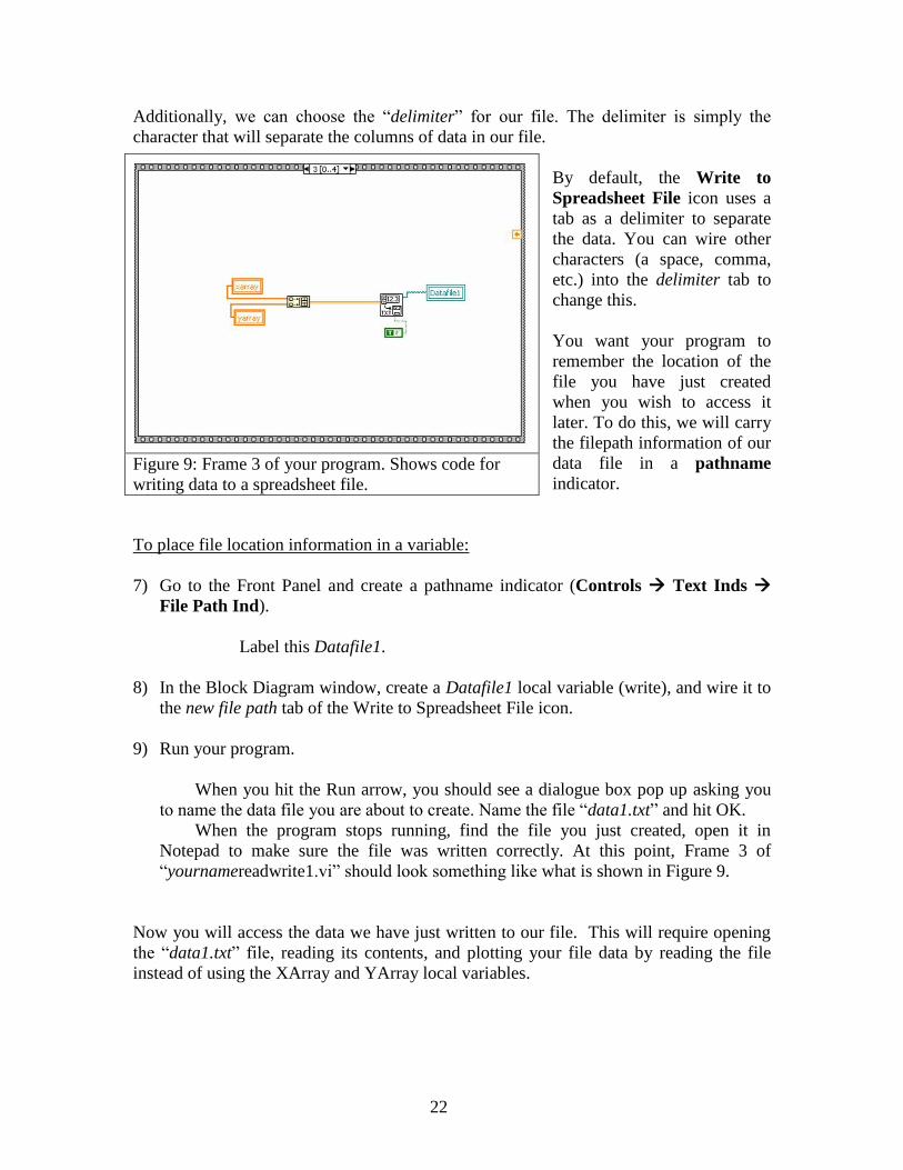
Additionally, we can choose the “delimiter” for our file. The delimiter is simply the

character that will separate the columns of data in our file.

By default, the Write to

Spreadsheet File icon uses a

tab as a delimiter to separate

the data. You can wire other

characters (a space, comma,

etc.) into the delimiter tab to

change this.

You want your program to

remember the location of the

file you have just created

when you wish to access it

later. To do this, we will carry

the filepath information of our

data file in a pathname

indicator.

To place file location information in a variable:

7) Go to the Front Panel and create a pathname indicator (Controls Text Inds

File Path Ind).

Label this Datafile1.

8) In the Block Diagram window, create a Datafile1 local variable (write), and wire it to

the new file path tab of the Write to Spreadsheet File icon.

9) Run your program.

When you hit the Run arrow, you should see a dialogue box pop up asking you

to name the data file you are about to create. Name the file “data1.txt” and hit OK.

When the program stops running, find the file you just created, open it in

Notepad to make sure the file was written correctly. At this point, Frame 3 of

“yournamereadwrite1.vi” should look something like what is shown in Figure 9.

Now you will access the data we have just written to our file. This will require opening

the “data1.txt” file, reading its contents, and plotting your file data by reading the file

instead of using the XArray and YArray local variables.

Figure 9: Frame 3 of your program. Shows code for

writing data to a spreadsheet file.

23

10) In Frame 4, erase the XArray and YArray local variables, and in the All Functions

File I/O window, select Read From Spreadsheet File.

Place the icon in Frame 4. Since the data stored in our file is of type Double (non-

integer numbers), leave the default option in the drop down selector.

You will need to tell Labview what file to read from. Instead of manually choosing the

file, you can just use the local variable we created in Frame 3!

11) Create a local variable (read) of Datafile1, and wire it into the file path input tab.

Make sure you know that Labview understands what the delimiter is for your data

file. If you choose to use commas as a delimiter when you create your text file, you

will have to tell Labview this when you try to open the file up and read data from it.

Because you chose the default delimiter (tab), you can leave this tab in its default

position, i.e. unwired, because this also signifies to use a tab delimiter when reading.

Note: because the data was transposed going into the file (so that the data could

be displayed in columns), you will want to transpose the data coming out of our file,

so that we are working with rows again. Figure out how to do this.

You will also need to separate the x-data from the y-data in the array we recover from

the file. After the data is read and transposed from the file, the output is an array of two

rows, each with “xsteps” number of columns. In order to make our graph function work,

we will need to extract our x-data and y-data, and then plug them into the XYGraph

function (through the Bundle).

12) Go to Programming Array Index Array. Place two icons in Frame 4 and

wire the array output of the Read From Spreadsheet File icon to the array input tab

of both.

To understand how Index Array works, we first must understand the data we are

trying to manipulate. The output of the Read From Spreadsheet File icon is a

double orange line, indicating it is an array of more than 1 dimension (Note: a normal

numeric is a single orange line, while a 1D array is a bold orange line). In our case,

we have a 2D array, with 2 rows (the “x” and “y” values), each containing “xsteps”

numbers. We would like to extract two different 1D arrays of length “xsteps,” one

containing the “x” values and one containing the “y” values.

The data in our 2D array is referenced using indices. There are two indices, each

representing some point along one of the two dimensions. So, for example, the 5th

“y”

value would have an index location of [1,4] (remember that we start counting from 0).

The Index Array function extracts the data at a given index. The number of input

indices is variable. If we input the indices 1 and 4, we will get back a number

corresponding to the 5th

“y” value. However, if we just put in the index 1, we will get

back a 1D array containing all the “y” values.

24

13) Wire the appropriate numeric constants to the index input on the Index Array icons.

Wire the two outputs to the two bundle inputs.

Because our x-axis data is the 0th

row, inputting “0’ to the “index” tab tells the

Index Array icon to take the “x” column. Inputting “1” to the other icon’s “index”

tab selects the y-axis.

Your Frame 4 should now look like that shown in Figure 10.

14) Save your program, and save another copy as “yournamereadwrite2.vi” to use next.

At this point you have been able perform basic read/write operations with spreadsheet

files. Spreadsheet files take arrays as input.

You may want to use strings to store information. Strings are simply variables consisting

of characters, using ASCII to encode the values into bits. In order to get some practice

using strings, you will now adjust our “yournamereadwrite1.vi” (now saved as

“yournamereadwrite2.vi”) to input the data as strings, not numbers. Additionally, you

will do this row by row, instead of saving your data column by column.

Figure 10: Block diagram for frame 4 of “yournamereadwrite1.vi”. Data is read from the

file “Datafile1”, transposed, and read into the XYGraph icon.

25

Some modifications will have to be made to the program in order to build our next file

row by row. More specifically, we will merge Frames 1 and 2, so that we build our x-

array and y-array simultaneously.

In addition to building the arrays simultaneously, we will also write each array line to file

as it’s built, instead of all at once after the arrays have been created. You will want to

create the data file before we get to the For Loop since you don’t want to open a dialogue

box each time through the For Loop.

15) Place the Programming File I/O Write to Text File icon in “Frame 0”

16) On the Front Panel, create a string input (Controls Express Text Ctrls

String Ctrl), and label it “Description”.

This string will serve as a header for the data file. Headers are located at the very

top of a file and typically provide information about the contents.

17) In the Block Diagram window, create a local variable (read) of the “description”

string. Place Concatenate String and End of Line Constant icons (All Functions

String) in the frame.

18) Wire the “description” local variable to the top left tab of the Concatenate String

icon, and wire the End of Line Constant icon to the bottom left tab.

The Concatenate String icon basically acts as an addition operator but for strings

instead of numbers.

19) Wire the output of the Concatenate String icon to the input of the Write Characters

to File icon.

We now have a program that will ask the user to select or create a file and write

our header to that file. We later want to write our arrays to that file, so we must record

where that file is located.

To do so, we will introduce the concept of a “refnum,” which is a number that

corresponds to a specific file path. Many of the File I/O functions use a refnum

input/output rather than a filepath input/output. For example, our Write Characters

to File icon outputs the refnum of the created file.

20) Use Programming File I/O Advanced File Functions Refnum to Path to

write the filepath to a Datafile1 local variable (write). Also, wire the refnum to a

Sequence Local to access it in other frames.

We now have access to either the pathname or refnum of our created file for use

elsewhere in our program.

26

21) Copy the Case Structure from Frame 2, and paste it into the For Loop of Frame 1.

22) Create an “f(x)” local variable (read) and wire it to the input of the Case Structure.

Wire the value of x(i) to the input tunnel of the Case Structure.

23) Build the y-array using a Build Array icon and a Shift Register, in a similar manner

to how you built the x-array in the same For Loop.

24) Delete Frame 2 (after you have a structure that can build the YArray in Frame 1) by

right-clicking on the border of Frame 2 and selecting Delete this Frame.

Next, we are going to use the For Loop to write to the file, line by line. In order to write

to a text file, the numbers must be changed to strings.

25) Place two Number to Engineering Strings (Programming String

String/Number Conversion) icons in the Frame 1 For Loop.

26) Wire x(i) into one of the “number” inputs, and y(i) into the other input.

The outputs of these icons are the numbers, but in string format.

27) Place a new Concatenate Strings (Programming String) icon near the Number

to Engineering String icons and expand it to have 4 inputs.

28) From top to bottom, wire into the Concatenate Strings inputs:

a. the output of the x(i) Number to Engineering String icon,

b. a Tab Constant, i.e. a tab string constant (Programming String),

Figure 11: Frame 0 after creating a new file and adding a header.

27

c. the output of the y(i) Number to Engineering String icon, and

d. an End of Line Constant (Programming String).

29) Place a Write to Text File icon (Programming File I/O) in the For Loop and

wire the output of the Concatenate Strings icon to its input.

30) Wire the refnum Sequence Local to the file input of the Write to Text File icon.

28) Delete the last two Frames of your program, leaving only Frames 0 and 1.

Frame 1 should now look like the structure shown in Figure 12.

Figure 12: Frame 1 from “yournamereadwrite2.vi”. Data is written to a file in this case

as strings instead of as numbers.

Now you have written your data to your file as strings. Like your spreadsheet file, this

file can be read, the values extracted, and the data can then be used to create a graph. The

rest of the section will give you an outline of how to do this for your new file, but at this

point you should be able to figure out the specifics yourself.

31) Create a “Frame After” to be labeled Frame 2, and place a Read from Text File icon

(under File I/O) in the Frame.

32) Use a Search and Replace String to search for the header you previously added and

replace it with an Empty String Constant.

28

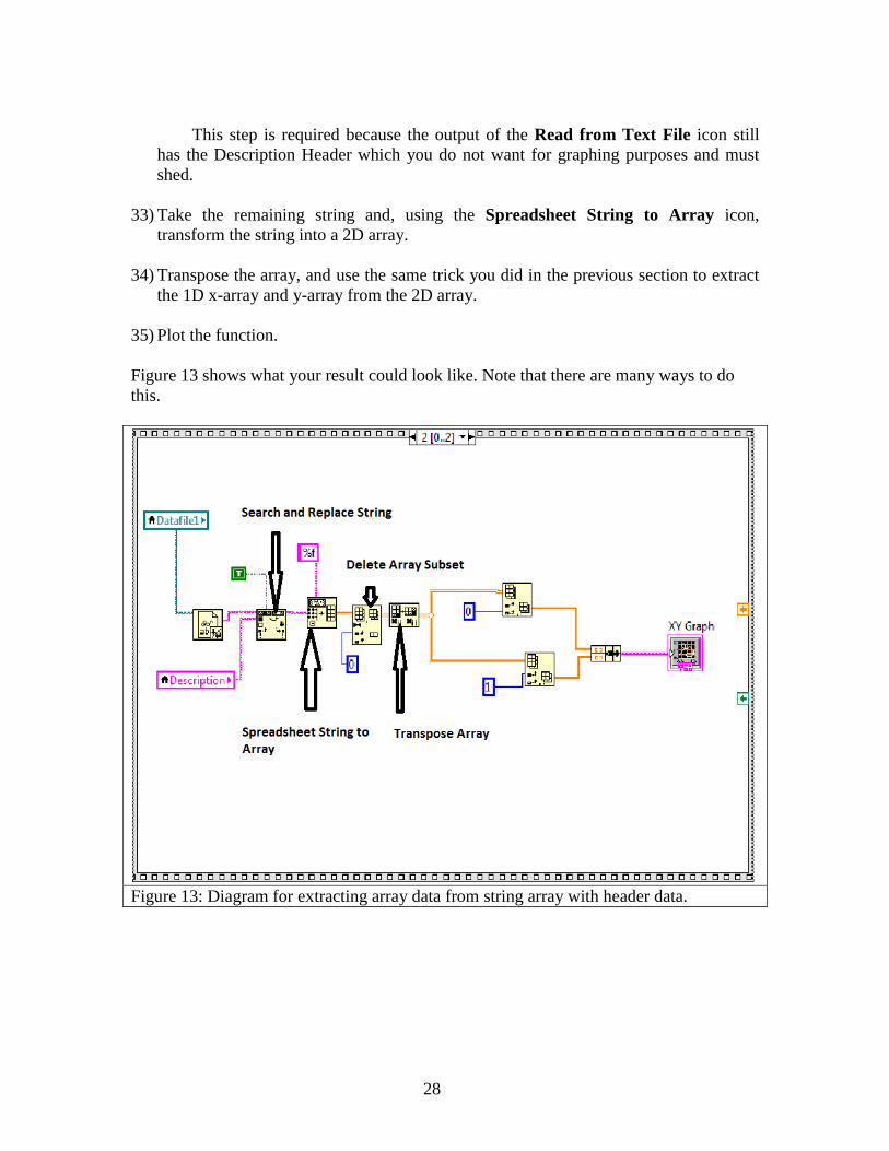
This step is required because the output of the Read from Text File icon still

has the Description Header which you do not want for graphing purposes and must

shed.

33) Take the remaining string and, using the Spreadsheet String to Array icon,

transform the string into a 2D array.

34) Transpose the array, and use the same trick you did in the previous section to extract

the 1D x-array and y-array from the 2D array.

35) Plot the function.

Figure 13 shows what your result could look like. Note that there are many ways to do

this.

Figure 13: Diagram for extracting array data from string array with header data.

29

VI) Troubleshooting

Labview has quite a few features which can help you when you run into problems with

your program. A few of the most helpful are listed below.

1) Running with a Broken Arrow:

If something is wrong with your program, the “Run” arrow is “broken”. The broken

arrow in place of the run button tells you that your program will not run.

A broken run arrow usually means that there is:

a) a broken wire,

b) a mis-wired icon, or

c) a data-type mismatch, i.e. trying to connect an string to a numeric indicator.

However, if you try to run with a broken arrow anyway, an error window will appear

with a list of the errors in the program. If you click on one of these errors, a longer

explanation of the error will appear in a lower window of the error dialogue box. If you

double-click on the error message the error will be highlighted in the block diagram so

that you can find it.

In Figure 14, there is a very simple For Loop with N = 10, using two variables, x and y.

The y variable is multiplied by the index i, and then the result is converted to a string and

written to a string indicator labeled “string”. The x variable is added to 2π and then wired

to the input of an array function called Reshape Array. Since the input of the Reshape

Array function is supposed to be an array, not a number, the program cannot run. This

can be seen by the broken arrow, but also by the red “X” through the wire connecting x +

2π to the Reshape Array function.

Figure 14: Error list generated by pressing on ‘broken’ run button when a scalar output is

connected to an array input.

30

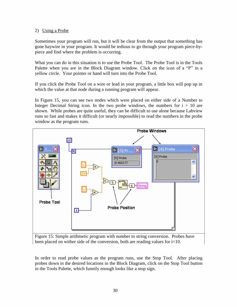
2) Using a Probe

Sometimes your program will run, but it will be clear from the output that something has

gone haywire in your program. It would be tedious to go through your program piece-by-

piece and find where the problem is occurring.

What you can do in this situation is to use the Probe Tool. The Probe Tool is in the Tools

Palette when you are in the Block Diagram window. Click on the icon of a “P” in a

yellow circle. Your pointer or hand will turn into the Probe Tool.

If you click the Probe Tool on a wire or lead in your program, a little box will pop up in

which the value at that node during a running program will appear.

In Figure 15, you can see two nodes which were placed on either side of a Number to

Integer Decimal String icon. In the two probe windows, the numbers for i = 10 are

shown. While probes are quite useful, they can be difficult to use alone because Labview

runs so fast and makes it difficult (or nearly impossible) to read the numbers in the probe

window as the program runs.

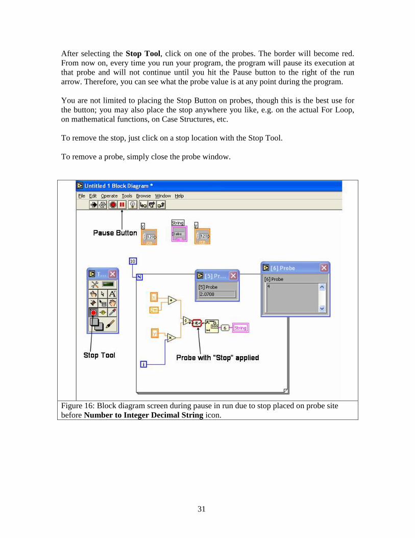
In order to read probe values as the program runs, use the Stop Tool. After placing

probes down in the desired locations in the Block Diagram, click on the Stop Tool button

in the Tools Palette, which funnily enough looks like a stop sign.

Figure 15: Simple arithmetic program with number to string conversion. Probes have

been placed on wither side of the conversion, both are reading values for i=10.

31

After selecting the Stop Tool, click on one of the probes. The border will become red.

From now on, every time you run your program, the program will pause its execution at

that probe and will not continue until you hit the Pause button to the right of the run

arrow. Therefore, you can see what the probe value is at any point during the program.

You are not limited to placing the Stop Button on probes, though this is the best use for

the button; you may also place the stop anywhere you like, e.g. on the actual For Loop,

on mathematical functions, on Case Structures, etc.

To remove the stop, just click on a stop location with the Stop Tool.

To remove a probe, simply close the probe window.

Figure 16: Block diagram screen during pause in run due to stop placed on probe site

before Number to Integer Decimal String icon.

32

3) Highlight Execution

The final tool for troubleshooting is the Highlight Execution button. This button lies

directly to the right of the Pause button on the Run toolbar.

If you select the Highlight Execution button before running your program, your program

will run in slow motion and you will be able to see the data as it travels along the wires in

your program. This button essentially puts a probe at every node and on every wire in

your program, allowing you to see everything in your program as it runs.

For a long program, it can be tiresome to troubleshoot using this method, especially if

you already have an idea as to where the bug might be. If you have no clue where your

problem might be, the highlight execution feature is especially helpful.

Figure 17: Frozen screen from program run using highlight execution feature.