LAB EXPERIMENTS USING NI ELVIS II AND NI...

Lab 6: Transient Responses of Second-Order RLC Circuits

LAB EXPERIMENTS USING

NI ELVIS II AND NI MULTISIM

Alexander Ganago Jason Lee Sleight

University of Michigan

Ann Arbor

Lab 6 Transient Responses of Second-Order RLC

Circuits

© 2010 A. Ganago Introduction of 7


Goals for Lab 6 Learn about:

• Responses of second-order series RLC circuit to square-wave input signal o Three types of responses o Relationship between theoretical parameters α and ωB0B and the values of

resistance, inductance, and capacitance in the circuit o How can you tell what type of response is observed in the lab o Total losses of energy in the circuit o Parameters of damped oscillations

• Variable capacitors • Parasitic capacitance and resistance of the circuit

Calculate the parameters of responses of a series RLC circuit Simulate the responses of a series RLC circuit to square wave input signal Build a second-order circuit with a variable capacitor and variable resistor Measure the responses of the series RLC circuit to square-wave input Collect data for three types of responses at several settings of resistance and capacitance

in the circuit Compare your lab data to your calculations and simulation results Draw conclusions on the values and importance of the parasitic capacitance and resistance in your circuit.



Introduction If a circuit contains one capacitor or one inductor in addition to resistors, sources and op amps, its transient responses are explained with first-order differential equations; therefore, it is called a first-order circuit. The transients occur because capacitors and inductors store energy. In a circuit with one energy-storing element, the transients are always exponential, in the form of either monotonic decay or monotonic rise. This is what you learned in Lab 5. If a circuit contains two energy-storing elements, they can exchange the stored energy, which may lead to oscillations. The actual form of responses depends on the damping in the circuit: if a large part of the stored energy is lost as heat every period, the damping is high and oscillations do not occur. If the loss of energy is relatively small, damping is low and oscillations take place but their amplitude exponentially decreases with time (damped oscillations). Transient responses of such circuits are explained with second-order differential equations; therefore, we call them second-order circuits. In this lab, you will work with a series RLC circuit whose transient responses are thoroughly explained in the textbook. The general form of the second-order differential equation is:

22

02

d x dx2 xdt dt

α ω+ ⋅ ⋅ + ⋅ = f (t)

Here x is voltage or current in the circuit (in this lab, you will measure the capacitor voltage VBCB) and f(t) is the forcing function, which is (in this lab) either zero or a constant. When we use a square waveform for the forcing function, at any moment of time we can consider it a constant, although the value of that constant abruptly changes twice every period.

As great French mathematicians found about 200 years ago, this differential equation has three types of solutions, depending on the relative values of the two parameters—the damping factor α and the frequency of undamped oscillations ωB0B:

(1) if α < ωB0B, the response is so-called under-damped, including damped oscillations:

( ) ( ) ( )t1 d 2 dx(t) K cos t K sin t Ke αω ω − ⋅⎡ ⎤= ⋅ ⋅ + ⋅ ⋅ ⋅ +⎣ ⎦ 3

Here KB1B, KB2B, and KB3B are constants (independent of time), and 2 2d 0ω ω α= − is

the frequency of damped oscillations.



The amplitude of oscillations decreases exponentially with the time constant equal

to 1α

; thus, as you learned in Lab 5, after a time interval of 5α

their amplitude

will drop to below 1% of the initial value.

(2) if α > ωB0B, the response is so called over-damped, expressed as a sum of two decaying exponents:

( ) ( )2 22 20 0

4 5x(t) K K Ke eα α ω α α ω− − − − + −

= ⋅ + ⋅ + 6 Here KB4B, KB5B, and KB6B are constants (independent of time). This decay has no oscillations; it gets slower and slower as α increases.

(3) if α = ωB0B, the response is so called critically damped, expressed as:

( ) ( )t t7 8x(t) K K t Ke eα α− ⋅ − ⋅= ⋅ + ⋅ ⋅ + 9

Here KB7B, KB8B, and KB9B are constants (independent of time). This decay does not have oscillations; it is faster than the decay in the over-

damped case.

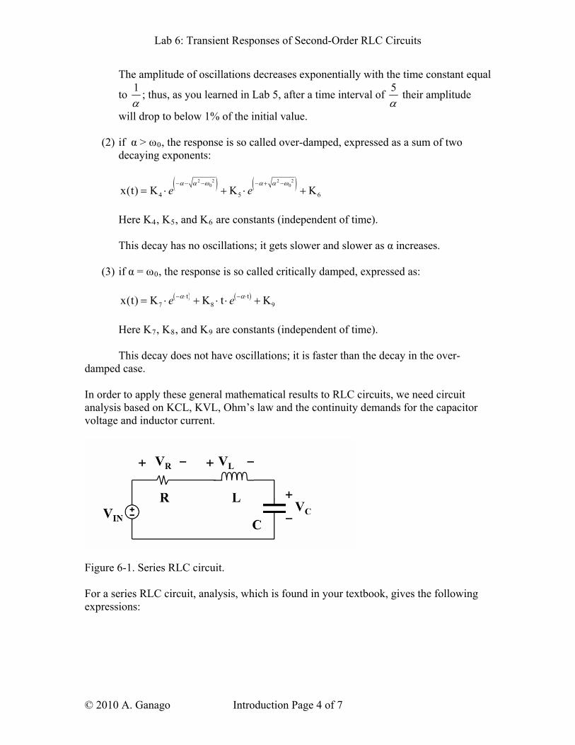
In order to apply these general mathematical results to RLC circuits, we need circuit analysis based on KCL, KVL, Ohm’s law and the continuity demands for the capacitor voltage and inductor current.

Figure 6-1. Series RLC circuit. For a series RLC circuit, analysis, which is found in your textbook, gives the following expressions:



0

R 2 L

1L C

α

ω

=⋅

=⋅

Note that circuit analysis is the key: for example, in a parallel RLC circuit the expression for ωB0B is the same but the expression for α is different! The constants KB1B through KB9B should also be found from the circuit analysis. The series RLC circuit is advantageous for experimental studies of the transients: firstly, it is simple to build and work on; secondly, its parameters α and ωB0B can be independently adjusted. If you vary the resistance R, then α varies but ωB0B remains the same. If you vary the capacitance C, then ωB0B varies but α remains the same. In many other circuits, when you vary one component (R or C), it affects both α and ωB0B. In the lab, you will work with a series RLC circuit with a variable resistor (potentiometer) and a variable capacitor as shown in Figure 6-2.

Figure 6-2. A series RLC circuit with a variable resistor (potentiometer) and a variable capacitor. As the source, you will use the function generator producing a square wave. For the variable capacitor, you will use a tuning capacitor such as found in an old radio receiver. It has two sets of semicircular flat metal plates: one set (the stator) is firmly attached to the chassis, while the other set (the rotor) rotates if you turn the shaft. The effective capacitance depends on the area of their overlap, which is shaded in Figure 6-3.



Figure 6-3. Basic design of a variable (tuning) capacitor. Capacitance of a plane capacitor is directly proportional to the area of its plates. Therefore, when the overlap of the stator and rotor increases, the capacitance of a tuning capacitor gets larger, as sketched in Figure 6-4.

Figure 6-4. The capacitance of a tuning capacitor depends on the overlap of its plates. One of the interesting features of this lab is that some of your observations will seemingly defy the theory. In particular, you might expect zero capacitance when the plates do not overlap at all—but you will never achieve zero capacitance in the lab. As we emphasized in Lab 5, circuits without capacitors do not exist (outside theoretical calculations and textbooks) because each conductor, even a piece of wire, has capacitance. We used the capacitance meter (built in NI ELVIS II) to measure the effective capacitance of the variable capacitor, which we disconnected from our circuit, and found that it varied from the maximal value, which agrees with the nominal 430 pF, to the minimal value in the range of tens of pF but never to zero. Furthermore, if we know the inductance L and measure the frequency of damped oscillations and the rate of their decay, then we can calculate the effective capacitance of our circuit. From this calculation, we obtained a noticeably larger value than what we



measured with the capacitance meter (see above) because the inductor also contributes to the effective capacitance of the circuit. Indeed, an inductor has many loops of wire, tightly packed, thus its effective capacitance can be in the range of tens or even hundreds pF. Moreover, in the circuit with a capacitor, inductor, and a variable resistor (such as in Figure 6-2) you cannot reduce the total resistance to zero, because the inductor has DC resistance (it is built of a long, thin wire) that may range from several ohms to tens of ohms, depending on the type of inductor (those built for larger currents have smaller resistances). This resistance can be measured with an ohmmeter. The total losses of energy in an RLC circuit are larger than those calculated from electric resistances (even if you take into account the DC resistance of inductor and wires) because they also include losses in the magnetic core of the inductor, etc. Therefore, if you study the type of transient response, adjust the resistance to achieve the critically damped response, then disconnect the resistor from your circuit and measure it with an ohmmeter, its resistance will probably be lower than that you calculate from the theory. Last but not least, note that theory gives you frequencies ωB0B and ωBdB in radians per second (if you use L in henrys and C in farads), but in the lab you measure the frequency of damped oscillations fBdB in hertz. The relationship is:

ddf

2ωπ

= 2



Pre-Lab:

For all problems use the following circuit, with a 10 mH inductor:

Part 1. Parameters of Damped Oscillations in Series RLC Circuit Use C = 430 pF, the maximal capacitance.

a. Calculate and record ωB0B and fB0B. Clearly label the units of measure. b. Fill in the following table:

Frequency of damped oscillations

Resistance in the circuit

R

(kΩ)

Damping factor

α

(µsP

-1P)

Decay Time

5/α

(µs)

ωBdB (rad/s)

fBdB (kHz)

Period of damped

oscillations

1/fBdB

(µs)

# periods per 5/α

0.05

1

2

4

8

9

9.6

Show your work for R = 9 kΩ.

c. Calculate and record the resistance RBCRB, at which the response is critically damped.

© 2010 A. Ganago Pre-Lab Page 1 of 2


Part 2. Simulation of the Series RLC Circuit Responses Under Various Conditions

Use Multisim to simulate the response of the series RLC circuit with 10 mH inductor and 430 pF capacitor (maximal capacitance of the variable capacitor) to a 5 kHz, 1 VBPPKB square wave with 0 V DC offset and a 50% duty cycle. The output voltage should be taken across the capacitor. The required values of resistance are listed below.

For each simulation, make a printout that clearly displays the output waveform over 2–3 periods of the square wave.

If oscillations are observed, determine and record their period in µs and frequency in kHz; compare with your calculations in Pre-Lab Part 1 (above).

2.1. Maximal Capacitance, R = 1 kΩ (Pre-Lab Printout #1) Use C = 430 pF, the maximal capacitance.

2.2. Maximal Capacitance, R = 50 Ω (Pre-Lab Printout #2) R = 50 Ω is modeling the minimal resistance.

2.3. Maximal Capacitance, R = 9.6 kΩ (Pre-Lab Printout #3) R = 9.6 kΩ is modeling the resistance RBCRB that corresponds to critically damped response in the series RLC circuit with C = 430 pF and L = 10 mH. You should obtain a better accuracy for RBCR

Bin Pre-Lab Part 1.

2.4. Maximal Capacitance, R = 111 kΩ (Pre-Lab Printout #4) R = 111 kΩ is modeling the maximal resistance in the circuit, which you will build in the lab.

© 2010 A. Ganago Pre-Lab Page 2 of 2


In-Lab Work IMPORTANT NOTES:

1. For this lab, disable channel 0 of the oscilloscope. This will increase the sampling rate on channel 1 and give you a smoother, more accurate signal.

2. When measuring the period of oscillations, you can achieve higher accuracy by positioning the cursors not on the adjacent peaks but several (n) periods apart, measure the time interval Δt between the cursors, and determine the period as

TTnΔ

=

The Circuit Turn on the NI ELVIS II.

From the NI ELVISmx Instrument launcher, launch the DMM VI.

Obtain a variable capacitor from your instructor and use the DMM to measure the maximum and minimum capacitance of your variable capacitor.

CBMAXB = ________ pF

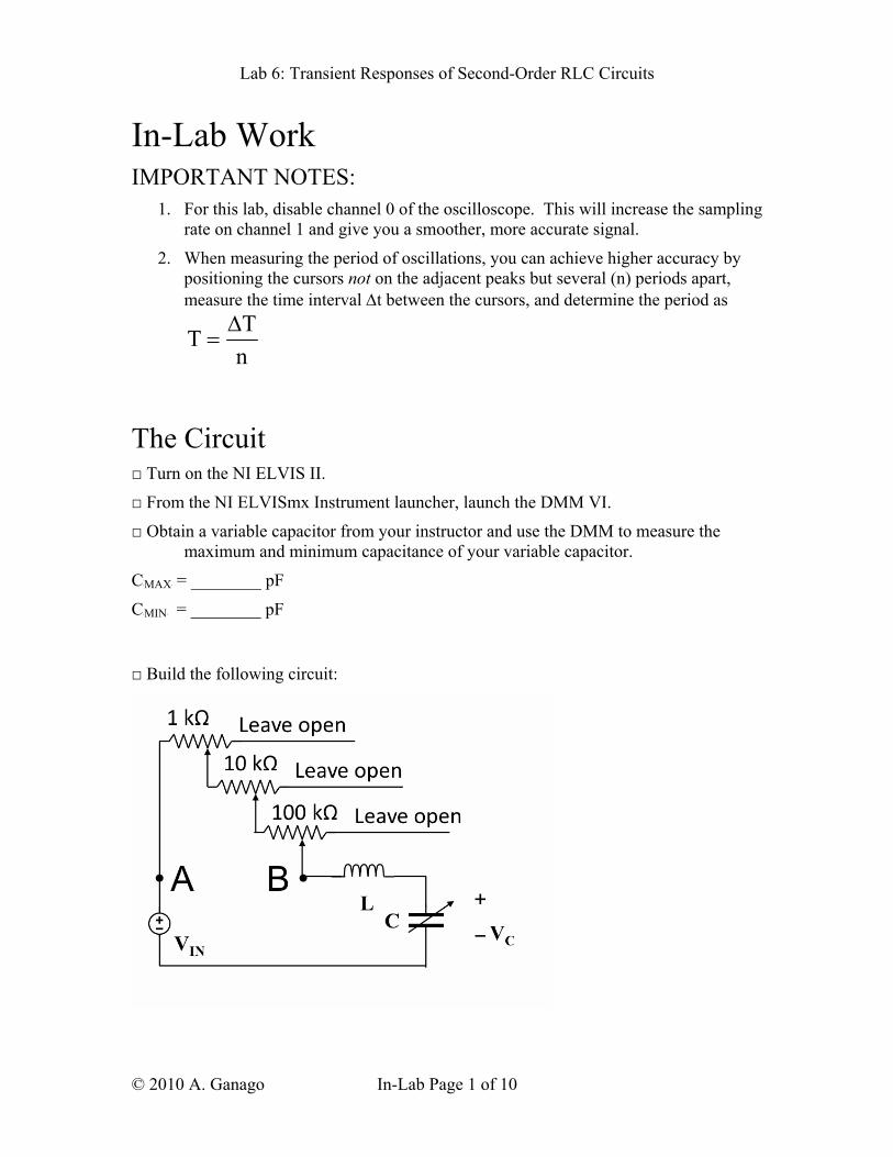
CBMINB = ________ pF Build the following circuit:

© 2010 A. Ganago In-Lab Page 1 of 10


Part 1. Under-Damped Response: Maximal Capacitance, R = 1 kΩ

Set the capacitor to its maximum value.

Set the 10 kΩ and 100 kΩ potentiometers to their minimal values, and the 1 kΩ potentiometer to its maximal value. This ensures the nominal resistance in the circuit equal to 1 kΩ.

From the NI ELVISmx Instrument launcher, launch the FGEN and OSCOPE VIs.

On the FGEN create a 5 kHz, 1 VBPPKB square wave with 0 V DC offset and 50% duty cycle.

Power on the PB.

Adjust the settings on the OSCOPE VI so that you can clearly view the waveform.

Use the cursors to measure the period TB1B of the oscillations, and then calculate fBd,1B.

TB1B = _________ μs fBd, 1B = _________ kHz

Create In-Lab Printout #1, which clearly shows the waveform. Click the log button to save a log of the data for use in the post-lab.



Part 2 Under-Damped Response: Maximal Capacitance, Minimal Resistance Set the 1 kΩ potentiometer to its minimal value. Keep the 10-kΩ and 100-kΩ

potentiometers at their minimal values as well. Keep the capacitor at its maximum value.

Adjust the setting on the OSCOPE VI so that you can clearly view the waveform.

Use the cursors to measure the period TB2B of the oscillations, and then calculate fBd, 2B.

TB2B = _________ μs fBd, 2B = _________ kHz




Part 3: Critically Damped Response Continue using the same circuit as in Part 1, repeated here for your convenience.

Leave the capacitor at its maximum value.

Slowly increase the value of the potentiometer(s), until you reach the critically damped response. You may want to begin by tuning the larger valued potentiometers and then tune the smaller ones. You may also want to zoom in on the relative section of the waveform in order to increase the accuracy of this measurement.

Create In-Lab Printout #3, which clearly displays the critically damped response. Click the log button to save a log of the data for use in the post-lab.

Carefully disconnect the potentiometers from the circuit (at nodes A and B, which are labeled with big dots on the circuit diagram from Part 1) and use the DMM to measure their combined resistance (between nodes A and B).

RBCR, LabB = ________ kΩ

Reconnect the potentiometers to the circuit.

If you choose to do extra credit explorations, see the assignment on the next page.

If do not plan explorations, go to Part 4.



Explorations (Part 3), for Extra Credit: The Effects of Capacitance on Damping Set the capacitor to its minimum value.

Notice how the response becomes under-damped without changing the resistance.

Adjust the parameters on the OSCOPE so that you can clearly view the oscillations.


TB3B = __________ μs

fBd, 3B = _________ kHz

Create In-Lab Printout #3-E, which clearly shows the waveform. Click the log button to save a log of the data for use in the post-lab.

Go to Part 4.



Part 4: Over-Damped Response Continue using the same circuit.

Set the capacitor at its maximum value.

Increase all the potentiometers to their maximum values.

Adjust the parameters on the OSCOPE VI so that the waveform is clearly visible.

Create In-Lab Printout #4 which clearly displays the over damped response. Click the log button to save a log of the data for use in the post-lab.


If do not plan explorations, go to Part 5.



Explorations (Part 4), for Extra Credit: The Effects of Capacitance on Damping (at Maximal Resistance) Set the capacitor to its minimum value.

Notice how the response becomes less damped without changing the resistance.

Adjust the parameters on the OSCOPE so that you can clearly view the waveform.

Create a printout which clearly shows the waveform. Click the log button to save a log of the data for use in the post-lab.

Go to Part 5.



Part 5: Varying Capacitance and Resistance Continue to use the same circuit.

Set the 1 kΩ potentiometer to its maximal value. Set the 10 kΩ and 100 kΩ potentiometers to their minimal values.

Set the capacitor to its maximal value. You should reproduce the result, which you obtained in the beginning of this lab (measurements of TB1B and fBd, 1B).

THE RESULT IS REPRODUCED Yes / No (circle one)

If all is done correctly and the result is reproduced, there is no need to record it again.

Set the capacitor to its minimum value.

Adjust the parameters on the OSCOPE VI so that you can clearly view the waveform.


TB4B = __________ μs

fBd, 4B = _________ kHz


This is the end of the required in-lab work.


If do not plan explorations, please power off the PB and NI ELVIS II and clean up your workstation.



Explorations (Part 5), for Extra Credit: The Effective Parameters of the Circuit (at Minimal Resistance and Minimal Capacitance) Set the capacitance to minimum, and set all potentiometers to their minimal values. For these settings, from simple theory you might expect zero capacitance and zero resistance. However, in the real circuit, you should observe decaying oscillations because the circuit has its effective capacitance and effective resistance.

The goal of this exploration is to collect data, which would allow you to calculate the effective capacitance and the effective resistance of the circuit.

Create In-Lab Printout #5-E, which clearly shows the waveform. Click the log button to save a log of the data for use in the post-lab.

Measure the period TB5B of oscillations, then calculate the frequency fBd, 5B.

TB5B = __________ μs fBd, 5B = _________ kHz

Collect the data during one half-period of the square wave (zoom in as needed).

Position the cursor at the top of the highest peak and record its horizontal in μs and the maximal voltage in mV, then go to the next peak. Fill the table below:



Peak # Position, μs Maximal value, mV

1

2

3

4

5

6

7

8

9

10

11

12

13

14

15

This is the end of the lab. Please power off the PB and NI ELVIS II and clean up your workstation.



Post-Lab:

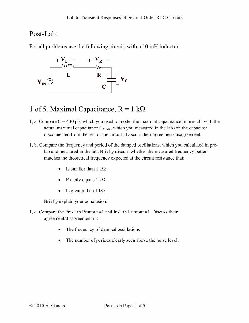
For all problems use the following circuit, with a 10 mH inductor:

1 of 5. Maximal Capacitance, R = 1 kΩ 1, a. Compare C = 430 pF, which you used to model the maximal capacitance in pre-lab, with the

actual maximal capacitance CBMAXB, which you measured in the lab (on the capacitor disconnected from the rest of the circuit). Discuss their agreement/disagreement.

1, b. Compare the frequency and period of the damped oscillations, which you calculated in pre-lab and measured in the lab. Briefly discuss whether the measured frequency better matches the theoretical frequency expected at the circuit resistance that:

• Is smaller than 1 kΩ

• Exactly equals 1 kΩ

• Is greater than 1 kΩ

Briefly explain your conclusion.

1, c. Compare the Pre-Lab Printout #1 and In-Lab Printout #1. Discuss their agreement/disagreement in:

• The frequency of damped oscillations

• The number of periods clearly seen above the noise level.

© 2010 A. Ganago Post-Lab Page 1 of 5


2 of 5. Maximal Capacitance, Minimal Resistance 2, a. Compare In-Lab Printout #1 and In-Lab Printout #2; list the differences between the

waveforms VBCB(t) and discuss whether they match your expectations based on Pre-Lab Printout #1 and Pre-Lab Printout #2.

2, b. Compare the Pre-Lab Printout #2 and In-Lab Printout #2. Discuss their agreement/disagreement in:



2, c. In pre-lab, R = 50 Ω is modeling the minimal resistance. Based on your comparison of the Pre-Lab Printout #2 and In-Lab Printout #2, determine whether the minimal resistance in the circuit, which you built in the lab, is larger or smaller than 50 Ω.



3 of 5. Maximal Capacitance, R = 9.6 kΩ 3, a. In Pre-Lab Part 1,c you calculated the resistance RBCRB that corresponds to critically damped

response in the series RLC circuit with C = 430 pF and L = 10 mH. In the lab (Part 3) you measured the actual value of RBCR, LabB that corresponds to the critically damped response in your circuit. Compare the values RBCRB and RBCR, Lab B; calculate their percentage difference

( )Measured Calculated100%

Calculated−

⋅

If it exceeds 1%, discuss the possible causes.

3, b. In the Pre-Lab (Part 2.3), you made Pre-Lab Printout #3 using R = 9.6 kΩ to model the resistance RBCRB that corresponds to critically damped response. In the lab, you made In-Lab Printout #3 of the critically-damped response. Compare the Pre-Lab Printout #3 and In-Lab Printout #3. Discuss their agreement/disagreement. Briefly comment.

3, c. EXPLORATION, FOR EXTRA CREDIT

In the lab, you kept the same resistance RBCR, LabB that corresponds to the critically-damped response in your circuit with maximal capacitance and reduced the capacitance to minimal. Discuss and explain the change of the type of response. Refer to In-Lab Printout #3 and In-Lab Printout #3-E.



4 of 5. Maximal Capacitance, R = 111 kΩ 4, a. Compare the Pre-Lab Printout #4, which you obtained with R = 111 kΩ, and In-Lab

Printout #4, which you obtained with the actual maximal resistance in your circuit. Discuss their agreement/disagreement in:

• The type of response

• The kinetics of the response

Also, discuss whether the circuit reaches (in your model and according to your lab data) a new DC steady state during each half-period of the square wave.

4, b. EXPLORATION, FOR EXTRA CREDIT

In the lab, you kept the same maximal resistance and reduced the capacitance to minimal. Refer to In-Lab Printout #4 and In-Lab Printout #4-E. Discuss and explain the change of the output waveform.



5 of 5. Varying Capacitance and Resistance 5, a. Compare the In-Lab Printout #1 (maximal capacitance, R = 1 kΩ) and In-Lab Printout #5

(minimal capacitance, R = 1 kΩ). Discuss and explain the change of the output waveform.

5, b. EXPLORATION, FOR EXTRA CREDIT

Compare the In-Lab Printout #3-E (minimal capacitance, R = RBCR, LabB) and In-Lab Printout #5 (minimal capacitance, R = 1 kΩ). Discuss their agreement/disagreement in:

• The type of response

• The kinetics of the response



Explain whether the distinctions match your expectations based on theory.

5, c. EXPLORATION, FOR EXTRA CREDIT

In the lab, you kept the same minimal capacitance and reduced the resistance to minimal. Refer to In-Lab Printout #5 and In-Lab Printout #5-E. Discuss and explain the change of the output waveform.

5, d. EXPLORATION, FOR EXTRA CREDIT

In the lab, you obtained In-Lab Printout 5-E kept with the minimal capacitance and resistance, and used the cursors to measure the position and voltage values of several peaks. Use these data to calculate the damping factor α and the frequency of damped oscillations fBdB and ωBdB. From α and ωBdB, calculate the frequency of undamped oscillations ωBoB. From α and ωB0B, calculate the effective minimal resistance RBEFF, MINB in ohms and the effective minimal capacitance CBEFF, MINB in pF of your circuit.

Discuss the agreement/disagreement between the purposed RBEFF, MINB and your actual RBEFF, MINB from the calculations. If there is a large discrepancy explain possible sources of error.

Compare the effective minimal capacitance CBEFF, MINB to the minimal capacitance of the variable capacitor, which you measured in the lab. Discuss the agreement/disagreement between the two capacitance values.


LAB EXPERIMENTS USING NI ELVIS II AND NI...

Documents

Transcript of LAB EXPERIMENTS USING NI ELVIS II AND NI...