Lab 7: Convection in a Turbulent Thermal Mixing Layer Objective: The objective of this laboratory is to become more familiar with the use of ANSYS ICEM CFD and FLUENT for solving convection heat transfer problems. Concepts introduced in this tutorial will include modeling turbulent flow, mesh adaptation, and the effects of numerical diffusion. Background: A thermal mixing layer occurs at the interface between cold and hot streams of fluid. This is a fundamental flow of great interest to a wide range of applications such as heat exchanger design, the mixing of contamination in the atmosphere and oceans, and the mixing of air and carbon dioxide above plants. In these examples, the diffusion and mixing of energy at a large scale are due primarily to turbulent motions, while molecular action is responsible for the diffusion and mixing at scales much smaller than the smallest turbulent eddies. Many researchers [1-4] have investigated these types of flows both experimentally and computationally in attempts to characterize important features such as the mixing layer growth rate. For this laboratory, we will simulate the thermal mixing layer flow shown schematically in Figure 1 that was investigated by LaRue and Libby [2]. The experiments were conducted in a wind tunnel approximately 0.8 m by 0.8 m in cross-section. A turbulence grid of 18 horizontal and 18 vertical rods is located at the inlet of the wind tunnel. The rods are separated by a spacing of M = 4.00 cm. The upper half of the rods are heated to make the flow in the top half of the wind tunnel a little higher in temperature than the flow in the bottom half of the wind tunnel. This small increase in temperature is used to mitigate effects due to buoyancy or variable properties so that just the turbulent mixing can be studied.

Figure 1. Schematic of thermal mixing layer created by a grid of rods (6 out of 18 shown) in a wind tunnel.

heated rods

unheated rods

y

x thermal mixing layer

x0 = 25 cm

Air at U = 7.65 m/s T∞ = 290 K

Air at U, Thot = 300 K

Air at U, T∞

M = 4.0 cm

2

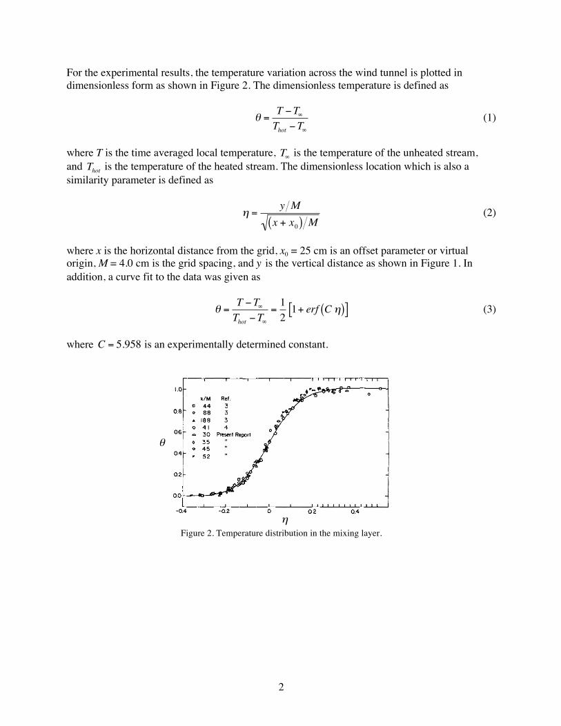
For the experimental results, the temperature variation across the wind tunnel is plotted in dimensionless form as shown in Figure 2. The dimensionless temperature is defined as

€

θ =T −T∞Thot −T∞

(1)

where T is the time averaged local temperature,

€

T∞ is the temperature of the unheated stream, and

€

Thot is the temperature of the heated stream. The dimensionless location which is also a similarity parameter is defined as

€

η =y M

x + x0( ) M (2)

where x is the horizontal distance from the grid, x0 = 25 cm is an offset parameter or virtual origin, M = 4.0 cm is the grid spacing, and

€

y is the vertical distance as shown in Figure 1. In addition, a curve fit to the data was given as

€

θ =T −T∞Thot −T∞

=121+ erf C η( )[ ] (3)

where

€

C = 5.958 is an experimentally determined constant.

Figure 2. Temperature distribution in the mixing layer.

η

θ

3

Figure 3. Schematic of computational domain. Laboratory: ANSYS ICEM CFD To run ICEM CFD, click on the ICEM CFD icon on the desktop. In the Main Menu, from the Settings pull down menu select Product Solver. In the DEZ verify under Product Setup Output Solver that ANSYS Fluent Solvers - CFD Version is selected. If it is not, do so, click OK, exit the program, and then restart ICEM CFD. Next, create (1) an unstructured mesh and (2) a structured mesh for two-dimensional slice shown in Figure 3 for the airflow in the wind tunnel by following the sequence of commands listed below. Create Unstructured Mesh Step 1. Select Working Directory and Create New Project Main Menu - Create a folder for your project. Do not use a name with spaces, including all the directories in the path. From File pull down menu, select Change Working Directory using LMB. In Browse for Folder dialog box select the folder you just created and click OK. Verify that the new working directory has been set in the Message Window. Main Menu - From File pull down menu, select New Project using LMB. In New Project dialog box create a new project. Again, do not use a name with spaces. Verify that your new project has been created in the Message Window. Step 2. Create Points for Geometry Function Tab - From Geometry select Create Point using LMB. DEZ - For Create Point enter the following: deselect Inherit Part (NOTE, this is only needed for Windows OS), in Part text edit box click LMB and enter PNT (replacing GEOM),

select Explicit Coordinates using LMB, under Explicit Locations ensure Create 1 point is selected from pull down menu,

Lx = 4.0 m

Ly = 0.8 m Ly/2

Ly/2

x

y

heated inlet

unheated inlet

pressure outlet walls

4

in X, Y, and Z text edit boxes ensure 0 is entered in each for point at (0, 0, 0), click Apply using LMB and verify the Message Done: points pnt.00, in Y text edit box click LMB and enter -0.4 for point at (0, -0.4, 0), click Apply using LMB and verify the Message Done: points pnt.01, in Y text edit box click LMB and enter 0.4 for point at (0, 0.4, 0), click Apply using LMB and verify the Message Done: points pnt.02, in X text edit box click LMB and enter 4 for point at (4, 0.4, 0), click Apply using LMB and verify the Message Done: points pnt.03, in Y text edit box click LMB and enter -0.4 for point at (4, -0.4, 0), click Apply using LMB and verify the Message Done: points pnt.04, click Dismiss using LMB.

Utilities - Select Fit Window using LMB to verify that 5 points have been created. DCT - Expand Geometry and Parts menus by using LMB to change + to - for each. Under Model\Geometry use RMB to click on Points and select Show Point Names using LMB. Verify that five points have been created. Step 3. Create Curves for Geometry

Function Tab - From Geometry select Create/Modify Curve using LMB. DEZ - For Create/Modify Curve enter the following: deselect Inherit Part (NOTE, this is only needed for Windows OS), in Part text edit box click LMB and enter INLET_COLD (replacing PNT),

select From Points using LMB, select Select location(s) using LMB (may not be needed if “Select locations with left button …” is already displayed at bottom of Graphics Window), select pnt.00 and pnt.01 using LMB and then click MMB to create unheated inlet, verify the Message Done: curves crv.00, in Part text edit box click LMB and enter INLET_HOT, select pnt.00 and pnt.02 using LMB and then click MMB to create heated inlet, verify the Message Done: curves crv.01, in Part text edit box click LMB and enter WALL, select pnt.01 and pnt.04 using LMB and then click MMB to create bottom wall, verify the Message Done: curves crv.02, select pnt.02 and pnt.03 using LMB and then click MMB to create upper wall, verify the Message Done: curves crv.03, in Part text edit box click LMB and enter OUTLET, select pnt.03 and pnt.04 using LMB and then click MMB to create upper outlet, verify the Message Done: curves crv.04, click DISMISS using LMB.

5

DCT - Under Model\Geometry use RMB to click on Points and unselect Show Point Names using LMB. Under Model\Geometry use RMB to click on Curves and select Show Curve Names using LMB and verify that five curves have been created as shown in Figure 4.

Figure 4. Point and curve names for unstructured mesh. Step 4. Create Surfaces for Airflow Function Tab - From Geometry select Create/Modify Surface using LMB. DEZ - For Create/Modify Surface enter the following: ensure Inherit Part is NOT selected, in Part text edit box click LMB and enter FLUID (replacing OUTLET),

select Simple Surface using LMB, under Surf Simple Method ensure From 2-4 Curves is selected from pull down menu, select Select curve(s) using LMB (may not be needed if “Select curves with left button…” is already displayed at bottom of Graphics Window), select crv.00, crv.01, crv.02, crv.03, and crv.04 using LMB and then click MMB, select APPLY using LMB to create surface for air flow, click DISMISS using LMB. NOTE: You will get a warning in the message window that the "number of selected curves is more than 4" and that the program is "attempting to create a bounded plane." DCT - Under Model\Geometry use RMB to click on Surfaces and select Show Surface Names using LMB and verify that one surface have been created the names srf.00. Step 5. Mesh Surface Using an Unstructured Mesh Function Tab - From Mesh select Surface Mesh Setup using LMB. DEZ - For Surface Mesh Setup enter the following: select Select Surface(s) using LMB, select srf.00 using LMB and then click MMB, in Maximum Size enter 0.04,

6

click Apply using LMB, click Dismiss using LMB. Function Tab - From Mesh select Compute Mesh using LMB. DEZ - For Compute Mesh enter the following:

in Compute select Compute Surface Mesh using LMB, check Overwrite Surface Preset/Default Mesh Type using LMB, in Mesh Type select All Tri from pull down menu using LMB, insure Overwrite Surface Preset/Default Mesh Method is not selected, click Compute using the LMB, and click Dismiss using LMB. NOTE: You should produce an unstructured mesh with triangular elements. Step 6. Save File, Export Unstructured Mesh, and Exit ICEM CFD Function Tab - From Output Mesh select Output To Fluent V6 Boundary Cond. using LMB. In Family Part boundary conditions dialog box: expand Edges and Mixed/unknown menus by using LMB to change + to -, expand INLET_COLD menu by using LMB to change + to -, click Create new to open the Selection dialog box, under Boundary Conditions select velocity-inlet using the LMB, click Okay using LMB to close the Selection dialog box, expand INLET_HOT menu by using LMB to change + to -, click Create new to open the Selection dialog box, under Boundary Conditions select velocity-inlet using the LMB, click Okay using LMB to close the Selection dialog box, expand OUTLET menu by using LMB to change + to -, click Create new to open the Selection dialog box, under Boundary Conditions select pressure-outlet using the LMB, click Okay using LMB to close the Selection dialog box, expand WALL menu by using LMB to change + to -, click Create new to open the Selection dialog box, under Boundary Conditions select wall using the LMB, click Okay using LMB to close the Selection dialog box, click Accept using LMB. Function Tab - From Output Mesh select Write Input using LMB. In Save dialog box click Yes using LMB to save current project first. In Open dialog box click Open to select unstructured mesh with current project name.

7

In ANSYS Fluent V6 dialog box enter the following: in Grid dimension select 2D using LMB, in Scaling ensure No is selected, in Write binary file ensure No is selected, in Ignore couplings ensure No is selected, in Boco file retain the default file name, in Output file change the file from fluent to a new name for your unstructured mesh, and click Done using LMB. Main Menu - From File pull down menu, select Exit using LMB. Create Structured Mesh In order to have a structured mesh that is aligned precisely with the cold and hot inlets we will create additional geometry. For this simple mesh the easiest way to do this is to start over. Step 1. Select Working Directory and Create New Project Restart ICEM CFD by clicking on the ICEM CFD icon on the desktop. Main Menu - From File pull down menu, select Change Working Directory using LMB. In New Project directory dialog box return to the directory used for your unstructured mesh. Main Menu - From File pull down menu, select New Project using LMB. In New Project dialog box create a new project. Again, do not use a name with spaces. Step 2. Create Points for Geometry Function Tab - From Geometry select Create Point using LMB. DEZ - For Create Point enter the following: ensure Inherit Part is NOT selected, in Part text edit box click LMB and enter PNT (replacing GEOM),

select Explicit Coordinates using LMB, under Explicit Locations ensure Create 1 point is selected from pull down menu, in X, Y, and Z text edit boxes ensure 0 is entered in each for point at (0, 0, 0), click Apply using LMB and verify the Message Done: points pnt.00, in Y text edit box click LMB and enter -0.4 for point at (0, -0.4, 0), click Apply using LMB and verify the Message Done: points pnt.01, in Y text edit box click LMB and enter 0.4 for point at (0, 0.4, 0), click Apply using LMB and verify the Message Done: points pnt.02, in X text edit box click LMB and enter 4 for point at (4, 0.4, 0), click Apply using LMB and verify the Message Done: points pnt.03, in Y text edit box click LMB and enter -0.4 for point at (4, -0.4, 0), click Apply using LMB and verify the Message Done: points pnt.04,

8

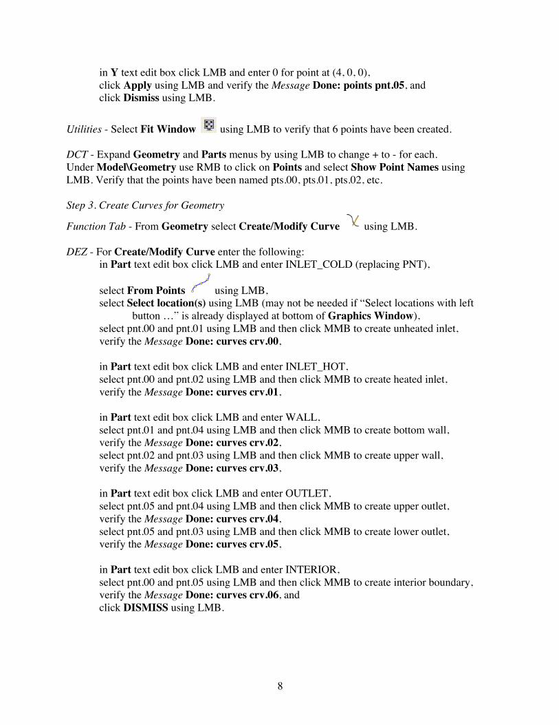
in Y text edit box click LMB and enter 0 for point at (4, 0, 0), click Apply using LMB and verify the Message Done: points pnt.05, and click Dismiss using LMB.

Utilities - Select Fit Window using LMB to verify that 6 points have been created. DCT - Expand Geometry and Parts menus by using LMB to change + to - for each. Under Model\Geometry use RMB to click on Points and select Show Point Names using LMB. Verify that the points have been named pts.00, pts.01, pts.02, etc. Step 3. Create Curves for Geometry

Function Tab - From Geometry select Create/Modify Curve using LMB. DEZ - For Create/Modify Curve enter the following: in Part text edit box click LMB and enter INLET_COLD (replacing PNT),

select From Points using LMB, select Select location(s) using LMB (may not be needed if “Select locations with left button …” is already displayed at bottom of Graphics Window), select pnt.00 and pnt.01 using LMB and then click MMB to create unheated inlet, verify the Message Done: curves crv.00, in Part text edit box click LMB and enter INLET_HOT, select pnt.00 and pnt.02 using LMB and then click MMB to create heated inlet, verify the Message Done: curves crv.01, in Part text edit box click LMB and enter WALL, select pnt.01 and pnt.04 using LMB and then click MMB to create bottom wall, verify the Message Done: curves crv.02, select pnt.02 and pnt.03 using LMB and then click MMB to create upper wall, verify the Message Done: curves crv.03, in Part text edit box click LMB and enter OUTLET, select pnt.05 and pnt.04 using LMB and then click MMB to create upper outlet, verify the Message Done: curves crv.04, select pnt.05 and pnt.03 using LMB and then click MMB to create lower outlet, verify the Message Done: curves crv.05, in Part text edit box click LMB and enter INTERIOR, select pnt.00 and pnt.05 using LMB and then click MMB to create interior boundary, verify the Message Done: curves crv.06, and click DISMISS using LMB.

9

DCT - Under Model\Geometry use RMB to click on Points and unselect Show Point Names using LMB. Under Model\Geometry use RMB to click on Curves and select Show Curve Names using LMB and verify that seven curves have been created as shown in Figure 5.

Figure 5. Point and curve names for structured mesh. Step 4. Create Surfaces for Airflow Function Tab - From Geometry select Create/Modify Surface using LMB. DEZ - For Create/Modify Surface enter the following: ensure Inherit Part is NOT selected, in Part text edit box click LMB and enter FLUID (replacing INTERIOR),

select Simple Surface using LMB, under Surf Simple Method ensure From 2-4 Curves is selected from pull down menu, select Select curve(s) using LMB (may not be needed if “Select curves with left button…” is already displayed at bottom of Graphics Window), select crv.00, crv.02, crv.04, and crv.06 using LMB and then click MMB, select APPLY using LMB to create lower surface for airflow, select Select curve(s) using LMB, select crv.01, crv.03, crv.05, and crv.06 using LMB and then click MMB, select APPLY using LMB to create upper surface for airflow, click DISMISS using LMB. DCT - Under Model\Geometry use RMB to click on Surfaces and select Show Surface Names using LMB and verify that two surfaces have been created with names srf.00 and srf.01. Step 5. Mesh Surface Using a Structured Mesh Function Tab - From Mesh select Surface Mesh Setup using LMB. DEZ - For Surface Mesh Setup enter the following: select Select Surface(s) using LMB, select srf.00 and srf.01 using LMB and then click MMB, in Maximum Size enter 0.04, click Apply using LMB,

crv.02

crv.03

crv.04

crv.05

10

click Dismiss using LMB.

Function Tab - From Mesh select Compute Mesh using LMB. DEZ - For Compute Mesh enter the following:

in Compute select Compute Surface Mesh using LMB, check Overwrite Surface Preset/Default Mesh Type using LMB, in Mesh Type select All Quad from pull down menu using LMB, check Overwrite Surface Preset/Default Mesh Method using LMB, in Mesh method select Autoblock from the pull-down menu, click Compute using the LMB, and click Dismiss using LMB. NOTE: You should produce a structured mesh with square elements. Step 6. Save File, Export Structured Mesh, and Exit ICEM CFD Function Tab - From Output Mesh select Output To Fluent V6 Boundary Cond. using LMB. In Family Part boundary conditions dialog box: expand Edges and Mixed/unknown menus by using LMB to change + to -, expand INLET_COLD menu by using LMB to change + to -, click Create new to open the Selection dialog box, under Boundary Conditions select velocity-inlet using the LMB, click Okay using LMB to close the Selection dialog box, expand INLET_HOT menu by using LMB to change + to -, click Create new to open the Selection dialog box, under Boundary Conditions select velocity-inlet using the LMB, click Okay using LMB to close the Selection dialog box, expand INTERIOR menu by using LMB to change + to -, click Create new to open the Selection dialog box, under Boundary Conditions select interior using the LMB, click Okay using LMB to close the Selection dialog box, expand OUTLET menu by using LMB to change + to -, click Create new to open the Selection dialog box, under Boundary Conditions select pressure-outlet using the LMB, click Okay using LMB to close the Selection dialog box, expand WALL menu by using LMB to change + to -, click Create new to open the Selection dialog box, under Boundary Conditions select wall using the LMB, click Okay using LMB to close the Selection dialog box, click Accept using LMB. Function Tab - From Output Mesh select Write Input using LMB. In Save dialog box click Yes using LMB to save current project first.

11

In Open dialog box click Open to select unstructured mesh with current project name. In ANSYS Fluent V6 dialog box enter the following: in Grid dimension select 2D using LMB, in Scaling ensure No is selected, in Write binary file ensure No is selected, in Ignore couplings ensure No is selected, in Boco file retain the default file name, in Output file change the file from fluent to a new name for your structured mesh, and click Done using LMB. Main Menu - From File pull down menu, select Exit using LMB. FLUENT Begin by launching FLUENT in 2-D, double precision mode then follow the steps below to set up a numerical model for the two-dimensional mixing layer simulation. Many of the detailed steps outlined in Lab 6 for problem setup are not repeated here. Step 1. Read In Mesh Import your unstructured mesh (first mesh created above) from ICEM CFD into FLUENT. Check to make sure the mesh imported correctly and is scaled correctly. Step 2. Problem Setup for Initial Simulation In the Navigation Pane Tree under Solution Setup use the following to setup your simulation: General: Solver • Type: Pressure-Based • Time: Steady • Velocity Formulation: Absolute • 2D Space: Planar Models (remaining models off) • Energy: On • Viscous (use defaults for coefficients and remaining options)

o Model: k-epsilon o k-epsilon Model: Realizable o Near-Wall Treatment: Standard Wall Functions

Materials (these are default values for air in materials database) • Density: 1.225 kg/m3 • Specific Heat: 1006.43 J/kg•K

12

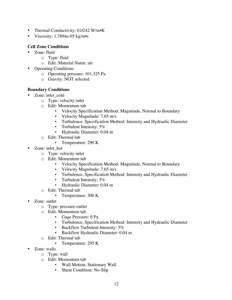
• Thermal Conductivity: 0.0242 W/m•K • Viscosity: 1.7894e-05 kg/m•s Cell Zone Conditions • Zone: fluid

o Type: fluid o Edit: Material Name: air

• Operating Conditions o Operating pressure: 101,325 Pa o Gravity: NOT selected

Boundary Conditions • Zone: inlet_cold

o Type: velocity-inlet o Edit: Momentum tab

• Velocity Specification Method: Magnitude, Normal to Boundary • Velocity Magnitude: 7.65 m/s • Turbulence, Specification Method: Intensity and Hydraulic Diameter • Turbulent Intensity: 5% • Hydraulic Diameter: 0.04 m

o Edit: Thermal tab • Temperature: 290 K

• Zone: inlet_hot o Type: velocity-inlet o Edit: Momentum tab

• Velocity Specification Method: Magnitude, Normal to Boundary • Velocity Magnitude: 7.65 m/s • Turbulence, Specification Method: Intensity and Hydraulic Diameter • Turbulent Intensity: 5% • Hydraulic Diameter: 0.04 m

o Edit: Thermal tab • Temperature: 300 K

• Zone: outlet o Type: pressure-outlet o Edit: Momentum tab

• Gage Pressure: 0 Pa • Turbulence, Specification Method: Intensity and Hydraulic Diameter • Backflow Turbulent Intensity: 5% • Backflow Hydraulic Diameter: 0.04 m

o Edit: Thermal tab • Temperature: 295 K

• Zone: walls o Type: wall o Edit: Momentum tab

• Wall Motion: Stationary Wall • Shear Condition: No-Slip

13

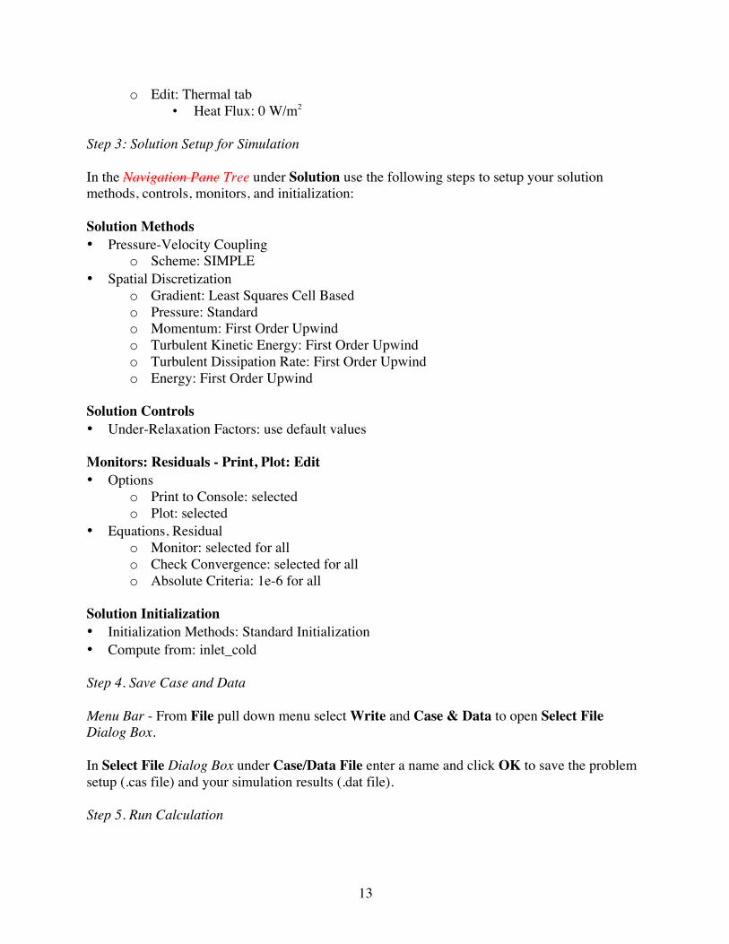
o Edit: Thermal tab • Heat Flux: 0 W/m2

Step 3: Solution Setup for Simulation In the Navigation Pane Tree under Solution use the following steps to setup your solution methods, controls, monitors, and initialization: Solution Methods • Pressure-Velocity Coupling

o Scheme: SIMPLE • Spatial Discretization

o Gradient: Least Squares Cell Based o Pressure: Standard o Momentum: First Order Upwind o Turbulent Kinetic Energy: First Order Upwind o Turbulent Dissipation Rate: First Order Upwind o Energy: First Order Upwind

Solution Controls • Under-Relaxation Factors: use default values Monitors: Residuals - Print, Plot: Edit • Options

o Print to Console: selected o Plot: selected

• Equations, Residual o Monitor: selected for all o Check Convergence: selected for all o Absolute Criteria: 1e-6 for all

Solution Initialization • Initialization Methods: Standard Initialization • Compute from: inlet_cold Step 4. Save Case and Data Menu Bar - From File pull down menu select Write and Case & Data to open Select File Dialog Box. In Select File Dialog Box under Case/Data File enter a name and click OK to save the problem setup (.cas file) and your simulation results (.dat file). Step 5. Run Calculation

14

In the Navigation Pane Tree under Solution: Run Calculation select Check Case. The only recommendation you should get back is that you should use higher order discretization. We will do this later so just close this window for now. Set the Number of Iterations to 200 steps and click Calculate. The problem should converge after about 170 steps. Repeat Step 4. Step 6. Make Contour Plots Visualize your results by displaying a contour plot of temperature for a temperature range of 290 K to 300 K. You should see a mixing layer in the middle between a layer of hot fluid on the top and cold fluid on the bottom. Use the Colormap Dialog Box to change the formatting for the temperature scale (Type: float, Precision: 1) to make it easier to read. Step 7. Define Dimensionless Parameters Use the following steps to create custom variables for the dimensionless parameters θ and η defined by Equations (1) and (2), respectively. They are needed to compare your simulation results to the experimental results given in the Background section: Menu Bar - From Define pull down menu select Custom Field Functions. In the Tree under Parameters & Customization right click on Custom Field Functions and select New… (or in the Ribbon select User-Defined tab and Create Custom Field Functions). In Custom Field Function Calculator Dialog Box enter the following: use the buttons to click ( , under Field Functions select Temperature from the pull down menu, click Select, use the buttons to click - , 2 , 9 , 0 , ) , / , 1 , and 0 , under New Function Name enter theta, click Define to define the dimensionless parameter θ, under Field Functions select Mesh and Y-Coordinate from the pull down menus, click Select, use the buttons to click / , 0 , . , 0 , 4 , / , SQRT , ( , ( , under Field Functions select Mesh and X-Coordinate from the pull down menus, click Select, use the buttons to click + , 0 , . , 2 , 5 , ) , / , 0 , . , 0 , 4 , ) , under New Function Name enter eta, click Define to define the dimensionless parameter η, and click Close to close the Custom Field Function Calculator Dialog Box. Note: In the Custom Field Function Calculator Dialog Box you can also click Manage to check each variable definition or to rename, delete, or save them. Step 8. Make xy Plots Menu Bar - From Surface pull down menu select Line/Rake.

15

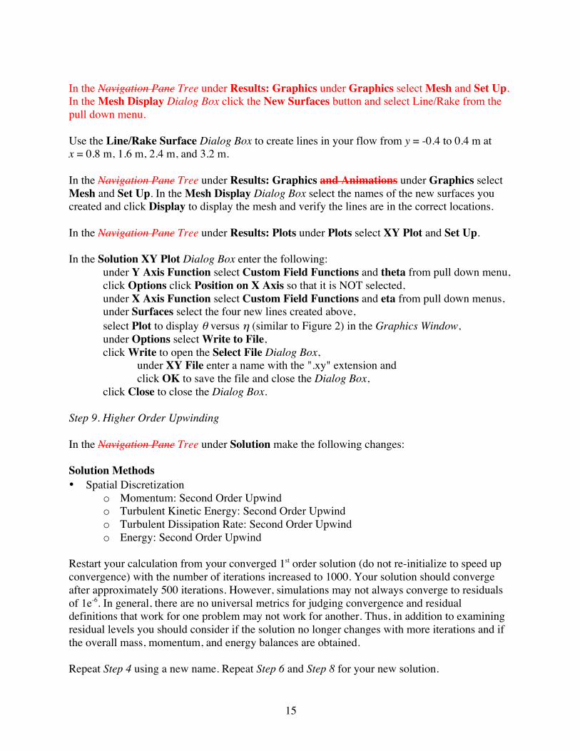
In the Navigation Pane Tree under Results: Graphics under Graphics select Mesh and Set Up. In the Mesh Display Dialog Box click the New Surfaces button and select Line/Rake from the pull down menu. Use the Line/Rake Surface Dialog Box to create lines in your flow from y = -0.4 to 0.4 m at x = 0.8 m, 1.6 m, 2.4 m, and 3.2 m. In the Navigation Pane Tree under Results: Graphics and Animations under Graphics select Mesh and Set Up. In the Mesh Display Dialog Box select the names of the new surfaces you created and click Display to display the mesh and verify the lines are in the correct locations. In the Navigation Pane Tree under Results: Plots under Plots select XY Plot and Set Up. In the Solution XY Plot Dialog Box enter the following: under Y Axis Function select Custom Field Functions and theta from pull down menu, click Options click Position on X Axis so that it is NOT selected, under X Axis Function select Custom Field Functions and eta from pull down menus, under Surfaces select the four new lines created above, select Plot to display θ versus η (similar to Figure 2) in the Graphics Window, under Options select Write to File, click Write to open the Select File Dialog Box, under XY File enter a name with the ".xy" extension and click OK to save the file and close the Dialog Box, click Close to close the Dialog Box. Step 9. Higher Order Upwinding In the Navigation Pane Tree under Solution make the following changes: Solution Methods • Spatial Discretization

o Momentum: Second Order Upwind o Turbulent Kinetic Energy: Second Order Upwind o Turbulent Dissipation Rate: Second Order Upwind o Energy: Second Order Upwind

Restart your calculation from your converged 1st order solution (do not re-initialize to speed up convergence) with the number of iterations increased to 1000. Your solution should converge after approximately 500 iterations. However, simulations may not always converge to residuals of 1e-6. In general, there are no universal metrics for judging convergence and residual definitions that work for one problem may not work for another. Thus, in addition to examining residual levels you should consider if the solution no longer changes with more iterations and if the overall mass, momentum, and energy balances are obtained. Repeat Step 4 using a new name. Repeat Step 6 and Step 8 for your new solution.

16

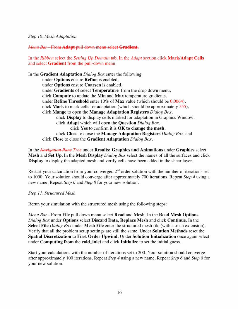
Step 10. Mesh Adaptation Menu Bar - From Adapt pull down menu select Gradient. In the Ribbon select the Setting Up Domain tab. In the Adapt section click Mark/Adapt Cells and select Gradient from the pull-down menu. In the Gradient Adaptation Dialog Box enter the following: under Options ensure Refine is enabled, under Options ensure Coarsen is enabled, under Gradients of select Temperature from the drop down menu, click Compute to update the Min and Max temperature gradients, under Refine Threshold enter 10% of Max value (which should be 0.0064), click Mark to mark cells for adaptation (which should be approximately 555), click Mange to open the Manage Adaptation Registers Dialog Box, click Display to display cells marked for adaptation in Graphics Window, click Adapt which will open the Question Dialog Box, click Yes to confirm it is OK to change the mesh, click Close to close the Manage Adaptation Registers Dialog Box, and click Close to close the Gradient Adaptation Dialog Box. In the Navigation Pane Tree under Results: Graphics and Animations under Graphics select Mesh and Set Up. In the Mesh Display Dialog Box select the names of all the surfaces and click Display to display the adapted mesh and verify cells have been added in the shear layer. Restart your calculation from your converged 2nd order solution with the number of iterations set to 1000. Your solution should converge after approximately 700 iterations. Repeat Step 4 using a new name. Repeat Step 6 and Step 8 for your new solution. Step 11. Structured Mesh Rerun your simulation with the structured mesh using the following steps: Menu Bar - From File pull down menu select Read and Mesh. In the Read Mesh Options Dialog Box under Options select Discard Data, Replace Mesh and click Continue. In the Select File Dialog Box under Mesh File enter the structured mesh file (with a .msh extension). Verify that all the problem setup settings are still the same. Under Solution Methods reset the Spatial Discretization to First Order Upwind. Under Solution Initialization once again select under Computing from the cold_inlet and click Initialize to set the initial guess. Start your calculations with the number of iterations set to 200. Your solution should converge after approximately 100 iterations. Repeat Step 4 using a new name. Repeat Step 6 and Step 8 for your new solution.

17

Assignment Submit plots of the following for the 2-D mixing layer case: 1. Structured mesh 2. Unstructured mesh 3. Adapted unstructured mesh 4. Contour plots of temperature for each of the cases considered: a. Unstructured mesh, first order upwind b. Unstructured mesh, second order upwind c. Adapted unstructured mesh, second order upwind d. Structured mesh, first order upwind For these contour plots, set the range to go from a minimum temperature of 290 K to a maximum temperature of 300 K by not selecting Auto Range and not selecting Clip to Range in the Contours Dialog Box. This will make the plots easy to compare. 5. Separate x/y plots of θ versus η (use a range of -0.5 to 0.5) at x = 0.8 m, 1.6 m, 2.4 m, and 3.2 m for each of the four cases above. On each plot include the curve fit to the experimental data given by Equation (3). Answer the following questions: 1. Calculate the Eckert number based on the temperature difference between the two streams and the velocity from the small inlet. Comment on whether it is reasonable to neglect viscous dissipation for this problem. 2. Calculate the Grashof number divided by the Reynolds number squared (Gr/Re2). Comment on whether it is reasonable to neglect natural convection for this problem. 3. Calculate the Mach number. Comment on whether it is reasonable to assume this problem is incompressible. 4. Comment on if it is reasonable to assume constant properties for this problem. 5. Describe numerical diffusion. Discuss how the contour plots from item 4 above are affected by numerical diffusion. Specifically, discuss how they change for higher order schemes, unstructured versus structured meshes, and mesh refinement. Calculate an average Peclet number using the diffusion coefficient for thermal energy and the average mesh spacing for each of the meshes. Use these results as part of your discussion. 6. Discuss your x/y plots from item 5 above. Comment on your ability to validate your results using the experimental correlation developed by LaRue and Libby.

18

References: [1] Elghobashi, S. E. and Launder, B. E., “Turbulent time scales and the dissipation rate of temperature variance in the thermal mixing layer,” Phys. Fluids, 26(9), April 1983. [2] LaRue, J. C., and Libby, P. A., “Thermal mixing layer downstream of half-heated turbulence grid,” Phys. Fluids, 24(4), April 1981. [3] LaRue, J. C., Libby, P. A., and Seshadri, V. R., “Further results on the thermal mixing layer downstream of a turbulence grid,” Phys. Fluids, 24(11), November 1981. [4] Macinnes, J. M., “Numerical simulation of the thermal turbulent mixing layer,” Phys. Fluids, 28(4), November 1985.