ECEN 3300 Linear Systems Spring 201004-12-10 P. Mathys

Lab 6: Convolution, Fourier Transforms, Ideal Filters,

and Applications (Second Draft)

1 Introduction

The (one-sided) Laplace and z transforms work very well for the analysis and design of causalCT and DT LTI systems with rational system functions that are characterized by their polesand zeros. For a high level description of signal processing and control systems, however, it isoften convenient to use idealized systems such as an ideal lowpass filter and leave the detailsof an actual implementation for later consideration at a lower level. As it turns out, suchidealized systems are typically noncausal and have impulse responses that are nonzero for alltimes t from −∞ to +∞. Thus, such systems cannot be designed and analyzed using (one-sided) Laplace and z transforms. A first step in the direction of formulating and analyzingideal LTI systems is to compute the response of a system directly in the time domain usingconvolution with integration or summation limits that extend from −∞ to +∞. In a secondstep Fourier transforms are then used to obtain a frequency domain characterization of ideal(and real) LTI systems. The CT Fourier transform (FT) and the DT Fourier transform(DTFT) are very similar to the Laplace and the z transforms, respectively, except that thescope in the transformed domain is restricted to the vertical axis in the s plane for CTsystems and to the unit circle in the z plane.

1.1 Discrete Time Convolution

Consider a DT LTI system with input xn ⇔ X(z), unit impulse response hn ⇔ H(z), andoutput yn ⇔ Y (z), where the X(z), H(z), and Y (z) are one-sided z-transforms. Start fromY (z) = X(z) H(z) and use the definition of the (one-sided) z transform to obtain

Y (z) =∞∑

m=−∞

xm um z−m

∞∑k=−∞

hk uk z−k =∞∑

m=−∞

∞∑k=−∞

xm um hk uk z−(m+k)

=∞∑

n=−∞

∞∑m=−∞

xm um hn−m un−m z−n =∞∑

n=0

n∑m=0

xm hn−m z−n ,

where the change of variable n← m + k (and thus k = n−m) was made. From this it canbe concluded that in the time domain

yn =n∑

m=0

xm hn−m = xm ∗ hn−m ,

1

i.e., yn is the convolution, denoted by ∗, of xn and hn. To accomodate two-sided sequences(and non-causal impulse responses) the summation limits are extended to ±∞ and thedefinition of DT convolution becomes

yn = xn ∗ hn =∞∑

m=−∞

xm hn−m =∞∑

k=−∞

hk xn−k = hn ∗ xn .

Note that DT convolution is commutative, i.e., xn ∗ hn = hn ∗ xn.

1.2 Continuous Time Convolution

Let h(t) ⇔ H(s) be the unit impulse response of a causal CT LTI system with inputx(t) ⇔ X(s) and output y(t) ⇔ Y (s), where H(s), X(s), and Y (s) are one-sided Laplacetransforms. Using the definition of the (one-sided) Laplace transform Y (s) = X(s) H(s) canbe written as

Y (s) =

∫ ∞

−∞x(τ) u(τ) e−sτ dτ

∫ ∞

−∞h(µ) u(µ) e−sµ dµ

=

∫ ∞

−∞

∫ ∞

−∞x(τ) u(τ) h(µ) u(µ) e−s(τ+µ) dτ dµ

=

∫ ∞

−∞

∫ ∞

−∞x(τ) u(τ) h(t− τ) u(t− τ) e−st dτ dt =

∫ ∞

0

∫ t

0

x(τ) h(t− τ) dτ e−st dt .

Thus, in the time domain,

y(t) =

∫ t

0

x(τ) h(t− τ) dτ = x(t) ∗ h(t) ,

i.e., y(t) is obtained as the convolution between x(t) and h(t). Extending this for all t from−∞ to +∞ yields the following definition for CT convolution

y(t) = x(t) ∗ h(t) =

∫ ∞

−∞x(τ) h(t− τ) dτ =

∫ ∞

−∞h(µ) x(t− µ) dµ = h(t) ∗ x(t) .

Note that CT convolution is commutative, i.e., x(t) ∗ h(t) = h(t) ∗ x(t).

1.3 Different Fourier Transforms

Fourier transforms are used to convert between time and frequency domain representationsof signals. Both time and frequency domain representations can be either continuous ordiscrete in the time and frequency variables. This results in a total of 4 different Fouriertransform variants as outlined in the table below.

2

Continuous Frequency (CF) Discrete Frequency (DF)

Continuous Time (CT)Fourier Transform

FTFourier Series

FS

Discrete Time (DT)Discrete Time

Fourier TransformDTFT

Discrete Fourier TransformFast Fourier Transform

DFT/FFT

The transform that is most general and easiest to work with analytically is the Fouriertransform (FT) with continuous time and frequency domains. The Fourier series (FS) canbe obtained from the FT by sampling in the frequency domain. The discrete time Fouriertransform (DTFT) is the dual of the FS and is obtained from the FT by sampling in thetime domain. Sampling in one domain implies periodicity in the other domain and thus timedomain signals for the FS are periodic with period T1, where f1 = 1/T1 is the fundamentalfrequency. Similarly, DTFT frequency domain represenations are periodic with period Fs,where Fs is the sampling rate. Finally, the discrete Fourier transform (DFT) and its compu-tationally fast implementation, the fast Fourier transform (FFT), can be derived from theFT by sampling in both the time and frequency domains. In this case, since the represen-tations in both domains are sampled, they are also both periodic in the blocklength of theDFT. One of the key features of the DFT is that it can be computed easily (for moderateblocklengths at least) numerically for arbitrary signals.

In all 4 cases the frequency domain expressions are complex-valued in general (even if thetime domain signals are real). Thus, it is necessary to display Fourier transforms in the formof two graphs, e.g., one for the magnitude and one for the phase.

1.4 Fourier Transform

Definition: The Fourier transform (FT) of a continuous time (CT) signal x(t) is defined as

X(f) =

∫ ∞

−∞x(t) e−j2πftdt ,

where f is frequency in Hz (sec−1).

Theorem: Inverse FT. A CT signal x(t) can be recovered uniquely from its FT X(f) by

x(t) =

∫ ∞

−∞X(f) ej2πftdf .

Time-Shift Property: Let x(t)⇔ X(f) be a FT pair. Then, using the inverse FT,

x(t− t0) =

∫ ∞

−∞X(f) ej2πf(t−t0)df =

∫ ∞

−∞X(f) e−j2πft0 ej2πftdf ,

3

so that x(t− t0)⇔ X(f) e−j2πf0t, where x(t− t0) is x(t) shifted to the right by t0.

Frequency-Shift Property: Let X(f)⇔ x(t) be a FT pair. Then, using the definition ofthe FT,

X(f − f0) =

∫ ∞

−∞x(t) e−j2π(f−f0)tdt =

∫ ∞

−∞x(t) ej2πf0t e−j2πftdt ,

so that X(f − f0)⇔ x(t) ej2πf0t, where X(f − f0) is X(f) shifted to the right by f0.

Example: Rectangular Pulse. Let

x(t) =

{1 , −τ/2 ≤ t < τ/2 ,0 , otherwise .

Then

X(f) =

∫ τ/2

−τ/2

e−j2πftdt =e−j2πft

−j2πf

∣∣∣τ/2

−τ/2=

e−jπfτ − ejπfτ

−j2πf=

sin πfτ

πf,

i.e., the FT of a rectangular pulse of width τ and amplitude 1 is a “sinc” pulse of amplitudeτ and main lobe of width 2/τ .

1.5 Fourier Series

Definition: The Fourier series (FS) of a periodic CT signal x(t) with period T1 is definedas

Xk =1

T1

∫T1

x(t) e−j2πkt/T1dt , k = 0,±1,±2, . . . ,

where the integration is taken over any interval of length T1. The FS coefficients Xk corre-spond to frequency components at fk = k/T1. Frequency f1 = 1/T1 is called the fundamentalfrequency, f2 = 2/T1 is called the 2’nd harmonic, f3 = 3/T1 is called the 3’rd harmonic, etc.

Theorem: Inverse FS. A periodic CT signal x(t) can be recovered uniquely from its FScoefficients Xk by

x(t) =∞∑

k=−∞

Xk ej2πkt/T1 ,

where T1 is the period of x(t).

FT of Periodic x(t). A periodic CT signal x(t) with period T1 can also be characterizedin the frquency domain in terms of a FT. Starting from its FS coefficients Xk, x(t) can beexpressed as

x(t) =∞∑

k=−∞

Xk ej2πkt/T1 .

Then, noting that the FT is a linear transformation, X(f) can be computed as

X(f) = F{x(t)} = F{ ∞∑

k=−∞

Xk ej2πkt/T1}

=∞∑

k=−∞

Xk F{ej2πkt/T1} =∞∑

k=−∞

Xk δ(f − k/T1) .

4

1.6 Discrete Time Fourier Transform

Definition: The discrete-time Fourier transform (DTFT) of a discrete time (DT) signal xn,n = 0,±1,±2, . . ., is defined as

X(φ) =∞∑

n=−∞

xn e−j2πφn ,

where φ is normalized (dimensionless) frequency. If Fs = 1/Ts is the sampling rate of thesequence xn, then φ = f/Fs, where f and Fs are frequencies in Hz. Note that X(φ) isperiodic in φ with period 1.

Theorem: Inverse DTFT. A DT signal xn, n = 0,±1,±2, . . ., can be recovered uniquelyfrom its DTFT X(φ) by

xn =

∫1

X(φ) ej2πφndφ ,

where the integration is taken over any interval of length 1.

Time-Shift Property: Let xn ⇔ X(φ) be a DTFT pair. Using the inverse DTFT

xn−m =

∫1

X(φ) ej2πφ(n−m) dφ =

∫1

X(φ) e−j2πφm ej2πφn dφ .

Therefore, xn−m ⇔ X(φ) e−j2πφm, where xn−m is xn shifted to the right by m.

Frequency-Shift Property: Let xn ⇔ X(φ) be a DTFT pair. Using the definition of theDTFT

X(φ− φ0) =∞∑

n=−∞

xn e−j2π(φ−φ0)n =∞∑

n=−∞

xn ej2πφ0n e−j2πφn .

Thus, X(φ− φ0)⇔ xn ej2πφ0n, where X(φ− φ0) is X(φ) shifted to the right by φ0.

Example: Rectangular DT Pulse. Let xn be the rectangular DT pulse of width dsamples and amplitde 1 shown in the following graph.

•••• • • •

• • •

xn

n0 1 2 d

1

↑d−1

· · ·

The DTFT of xn is

X(φ) =d−1∑n=0

e−j2πφn =1− e−j2πφd

1− e−j2πφ=

ejπφd − e−jπφd

ejπφ − e−jπφ

e−jπφd

e−jπφ=

sin πφd

sin πφe−jπφ(d−1) .

If d is an odd integer, then yn = x[n+d−12

] is the (symmetric around n=0) rectangular pulseof width d shown below.

5

•••••

• • •• • •

yn

n0 1 d+1

2-1-d+1

2

1

↑d−12

· · ·

-

↑d−12

· · ·

Using the time shift property, its DTFT is

Y (φ) = X(φ) ej2πφ(d−1)/2 =sin πφd

sin πφ.

1.7 Discrete Fourier Transform

Definition: The discrete Fourier transform (DFT) of a DT signal xn, n = 0, 1, . . . , N − 1(mod N), that is periodic with period N , is defined as

Xk =N−1∑n=0

xn e−j2πkn/N , k = 0, 1, . . . , N − 1 (mod N) .

Note that the sum can be taken over any N consecutive indexes. The term FFT (fast Fouriertransform) refers to a fast algorithm for computing the DFT for composite N and, very often,for the case when N is a power of 2.

Theorem: Inverse DFT/FFT. A periodic DT signal xn with period N can be recovereduniquely from the DFT coefficients Xk, k = 0, 1, . . . N − 1 (mod N), by

xn =1

N

N−1∑k=0

Xk ej2πkn/N , n = 0, 1, . . . , N − 1 (mod N) .

Note that the sum can be taken over any N consecutive indexes. The term inverse FFTrefers to a fast algorithm for computing the inverse DFT when N is composite, most oftenwhen N is a power of 2.

1.8 Approximation of Fourier Transform

The Fourier transform X(f) of a CT waveform x(t) is defined as

X(f) =

∫ ∞

−∞x(t) e−j2πft dt .

If x(t) is sampled at times t = nTs with a large enough sampling rate Fs = 1/Ts, then theintegral can be approximated by the sum

X(f) ≈∞∑

n=−∞

x(nTs) e−j2πfnTs Ts =1

Fs

X(φ) ,

6

where, using the notations x(nTs) = xn and fTs = f/Fs = φ,

X(φ) =∞∑

n=−∞

xne−j2πφn ,

is the DTFT of xn with normalized frequency φ. Note that X(φ) is periodic in φ with period1. In practice the samples xn of x(t) are only available for a finite range of n, e.g., forn = 0, 1, . . . , N − 1. Then

X(φ) =N−1∑n=0

xn e−j2πφn , 0 ≤ φ < 1 .

Now the question arises for which values of φ this should be computed. If xn is N -dimensionalin the time domain, then it should be possible to find a corresponding N -dimensional fre-quency domain representation. To explore this further, let xn = ej2πφ0n for some (normalized)frequency. Then

X(φ) =N−1∑n=0

ej2πφ0n e−j2πφn =N−1∑n=0

ej2π(φ0−φ)n =1− ej2π(φ0−φ)N

1− ej2π(φ0−φ).

If φ = φ0 then X(φ0) = N which is the maximum of X(φ) over all values of φ in the range0 . . . 1. If ej2π(φ0−φ)N = 1 and φ 6= φ0 then X(φ) = 0 and the complex exponentials ej2πφ0n

and e−j2πφn are orthogonal to each other for 0 ≤ n < N . This happens if (φ0 − φ)N = k orφ0−φ = k/N for k = 1, 2, . . . , N−1. Thus, if X(φ) is evaluated at φ0, then it should also beevaluated at φ = φ0 − k/N for k = 1, 2, . . . N − 1. Setting φ0 = (N − 1)/N , the frequenciesat which X(φ) should be computed are 0, 1/N, 2/N, . . . , (N − 1)/N . Thus, the computationof X(φ) for general xn can be rewritten as

X(k/N) =N−1∑n=0

xn e−j2πkn/N = Xk , k = 0, 1, . . . , N − 1 ,

where Xk are the DFT coefficients of the DT sequence xn, n = 0, 1, . . . , N − 1. Solvingφ = k/N = f/Fs for f yields f = kFs/N and thus the Fourier transform approximation forx(t) that is only available in the form of N equally spaced samples xn, n = 0, 1, . . . , N − 1with sampling rate Fs is

X(kFs/N) =1

Fs

N−1∑n=0

xn e−j2πkn/N =Xk

Fs

, k = 0, 1, . . . N − 1 ,

where Xk are the DFT coefficients of xn. If N is a composite number, then Xk can beevaluated using a fast Fourier transform (FFT). In Matlab the command fft can be usedfor this.

7

1.9 Ideal Filters

An ideal filter passes all frequencies in its passband(s) without attenuation and completelyrejects all frequencies outside its passband(s). The phase response of an ideal filter is either0 degrees or ±180 degrees for all frequencies. Thus, an ideal lowpass filter (LPF) with cutofffrequency fL and passband gain of 1 has frequency response

HL(f) =

{1 , 0 ≤ |f | < fL ,

0 , |f | > fL .

Computing the inverse Fourier transform yields

hL(t) =

∫ fL

−fL

ej2πftdf =ej2πft

j2πt

∣∣∣fL

−fL

=ej2πfLt − e−j2πfLt

j2πt=

sin 2πfLt

πt.

Thus, the unit impulse response of an ideal LPF with gain 1 and cutoff frequency fL is a“sinc” pulse with amplitude 2fL and main lobe of width 1/fL.

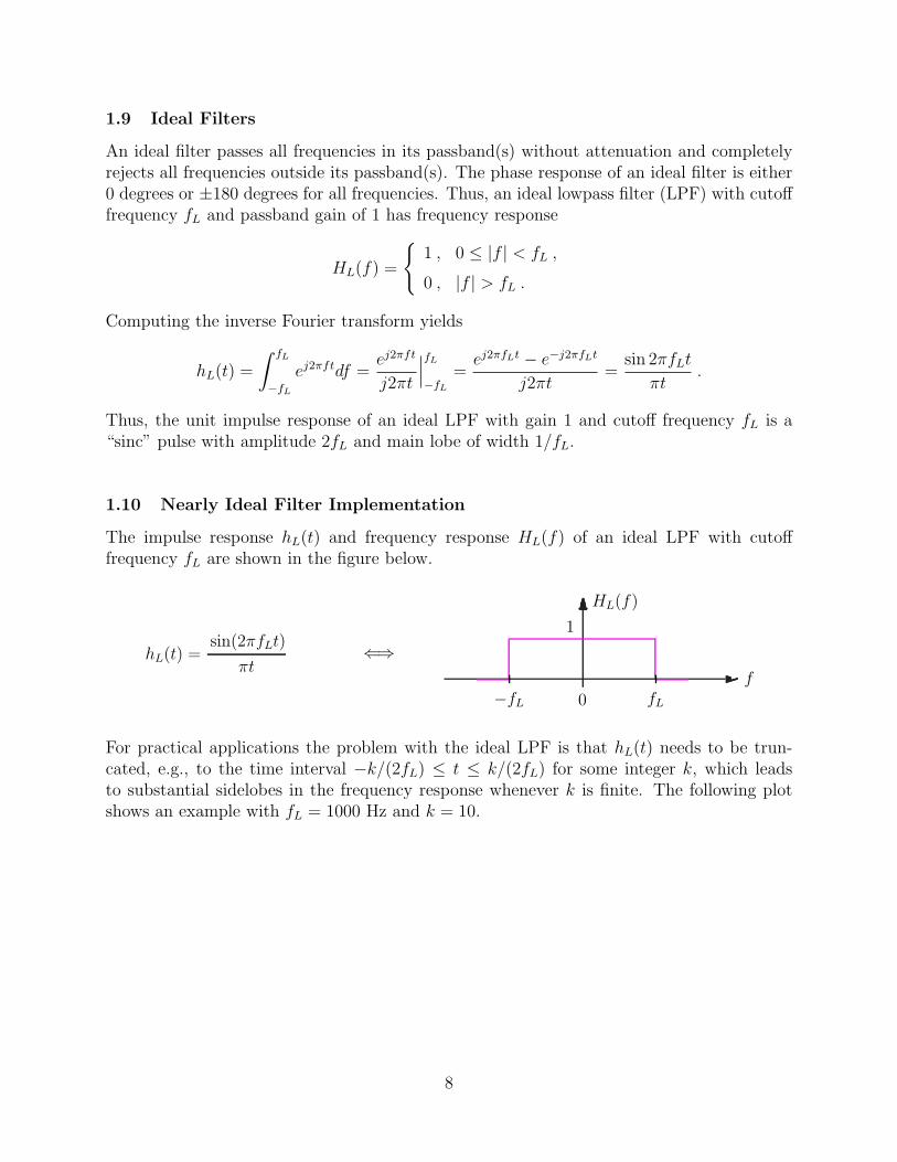
1.10 Nearly Ideal Filter Implementation

The impulse response hL(t) and frequency response HL(f) of an ideal LPF with cutofffrequency fL are shown in the figure below.

HL(f)

1

f−fL 0 fL

hL(t) =sin(2πfLt)

πt⇐⇒

For practical applications the problem with the ideal LPF is that hL(t) needs to be trun-cated, e.g., to the time interval −k/(2fL) ≤ t ≤ k/(2fL) for some integer k, which leadsto substantial sidelobes in the frequency response whenever k is finite. The following plotshows an example with fL = 1000 Hz and k = 10.

8

−5 −4 −3 −2 −1 0 1 2 3 4 5−500

0

500

1000

1500

2000

Ideal LPF, hL(t) Truncated to −k/(2f

L)<t<k/(2f

L), f

L=1000 Hz, k=10

t [ms]

h L(t)

−3000 −2000 −1000 0 1000 2000 3000−60

−50

−40

−30

−20

−10

0

f [Hz]

20*l

og10

(|H

L(f)|

) [d

B]

By making the transition from the passband to the stopband less abrupt, the situation canbe improved considerably. One way to achieve this is to convolve HL(f) with the rectangularspectrum P (f) with parameter 0 ≤ α ≤ 1 shown below.

P (f)1

2αfL

f−αfL 0 αfL

p(t) =sin(2παfLt)

2παfLt⇐⇒

In this way an overall frequency response of H(f) = HL(f)∗P (f) is obtained that has a lineartransition of width 2αfL from passband to stopband. In the time domain this corresponds toan overall impulse response h(t) = hL(t) p(t). As the parameter α is varied from 0 to 1, thefrequency response goes from an ideal LPF to a H(f) with triangular shape. An examplewith fL = 1000 Hz, k = 10, and α = 0.2 is shown below.

9

−5 −4 −3 −2 −1 0 1 2 3 4 5−500

0

500

1000

1500

2000

Trapezoidal LPF, hL(t) Truncated to −k/(2f

L)<t<k/(2f

L), f

L=1000 Hz, k=10, α=0.2

t [ms]

h L(t)

−3000 −2000 −1000 0 1000 2000 3000−60

−50

−40

−30

−20

−10

0

f [Hz]

20*l

og10

(|H

L(f)|

) [d

B]

If the magnitude of H(f) is plotted using a linear scale then it becomes evident that theconvolution of HL(f) with P (f) yields a filter with trapezoidal frequency response as shownbelow.

−3000 −2000 −1000 0 1000 2000 30000

0.2

0.4

0.6

0.8

1

1.2

1.4

f [Hz]

|HL(f

)|

Trapezoidal LPF, hL(t) Truncated to −k/(2f

L)<t<k/(2f

L), f

L=1000 Hz, k=10, α=0.2

1.11 Frequency Response Measurement

One way to measure the magnitude and the phase of a filter of interest is to sweep a sine anda cosine simultaneously from a frequency f1 to a frequency f2 and then use the blockdiagramshown below to compute the auxiliary quantities wi(t) and wq(t).

10

• Filterto Test

•

×

× LPFat fm

LPFat fm

2

-2

cos 2πft

sin 2πft

x(t) y(t)

vi(t)

vq(t)

wi(t)

wq(t)

If the response of the filter under test to x(t) = cos 2πft is of the form y(t) = A cos(2πft+θ),then

vi(t) = 2A cos(2πft + θ) cos(2πft) = A[cos θ + cos(4πft + θ)

],

vq(t) = −2A cos(2πft + θ) sin(2πft) = A[sin θ − sin(4πft + θ)

].

If the cutoff frequency fm of the LPFs is chosen such that the components of vi(t) and vq(t)at 2f are rejected, then

wi(t) = A cos θ , and wq(t) = A sin θ ,

and thus

|H(f)| = A =√

w2i (t) + w2

q(t) , and ∠H(f) = θ = tan−1(wq(t)

wi(t)

),

where H(f) is the frequency response of the filter under test.

Another approach to measure the frequency response of a filter under test is to use a unitimpulse at the input of the filter to produce the unit impulse response h(t) at the output.Then h(t) is sampled with sampling rate Fs, resulting in hn = h(nTs), n = 0, 1, . . . N − 1.Note that in Matlab hn is directly produced as the impulse response of a CT system simulatedby a DT system. Then the Fourier transform approximation

H(kFs/N) ≈ Hk

Fs

, k = 0, 1, . . . N − 1 ,

where Hk are the DFT coefficients of hn is used to compute the frequency response H(f) forf = kTs/N . The Hk can be evaluated using a FFT and then plots of |H(f)| and ∠H(f) atf = kTs/N can be made.

1.12 Application: Amplitude Modulation

As the name implies, amplitude modulation (AM) changes the amplitude of a carrier signalto transmit a message signal. More precisely, a AM signal x(t) can be obtained from amessage signal m(t) as

x(t) = Ac m(t) cos(2πfct) ,

11

where Ac is the carrier amplitude and fc is the carrier frequency in Hz. During transmissionthe AM signal is attenuated by a factor γ and thus the received signal is r(t) = γ x(t). Torecover m(t) from r(t), multiply with the local oscillator signal c(t) = 2 cos(2πfct) to obtain

v(t) = r(t) c(t) = γAc m(t) 2 cos2(2πfct)︸ ︷︷ ︸= 1 + cos(4πfct)

= γAc m(t) + γAc m(t) cos(4πfct)︸ ︷︷ ︸AM signal at 2fc

.

Thus, if v(t) is passed through a (ideal) lowpass filter that rejects the AM signal at 2fc, thenthe estimate of the received message signal is

m̂(t) = γAc m(t) ,

which is a scaled version of m(t). The generation of x(t) and the demodulation of r(t) areshown in the following block diagram.

×

Ac cos(2πfct)Carrier Oscillator

m(t)

x(t)

×

c(t) = 2 cos(2πfct)Local Oscillator

LPFat fL

r(t)

m̂(t)v(t)

Using the FT pairs

m(t) ⇐⇒ M(f) and cos(2πfct) ⇐⇒ δ(f − fc) + δ(f + fc)

2

the FT X(f) of x(t) is obtained as

X(f) = Ac M(f) ∗ δ(f − fc) + δ(f + fc)

2=

Ac

2

[M(f − fc) + M(f + fc)

].

Graphically, this can be represented as follows for the generic message FT M(f) shown onthe left.

M(f)

Mm

−fm 0 fm

f

X(f)

AcMm

2

−fc−fm

−fc

−fc+fm

0fc−fm

fc

fc+fm

f

LSB︷ ︸︸ ︷

USB︷ ︸︸ ︷

Note that if m(t) has no dc component, then there is no spectral component in x(t) at thecarrier frequency fc. Note further that the bandwidth of the baseband message signal m(t)

12

is fm, whereas the bandwidth of the AM signal x(t) is 2fm, i.e., the bandwidth doubles inthe process of going from m(t) to x(t). For this reason this form of amplitude modulationis called AM-DSB-SC (amplitude modulation, double sideband, suppressed carrier). Thespectral components in x(t) between fc−fm and fc are called the lower sideband (LSB) andthe spectral components between fc and fc + fm are called the upper sideband (USB) of theAM signal x(t).

—- To be completed —-

The block diagram of a AM-DSB-TC (amplitude modulation, double side-band, transmit-ted carrier) transmitter is shown in the following figure.

α

+ ×

Ac cos(2πfct + θc)Carrier Oscillator

1

mn(t)

1 + αmn(t) x(t)

Written out explicitly, the general form of a AM-DSB-TC signal is

x(t) = Ac

(1 + αmn(t)

)cos(2πfct + θc) = Ac cos(2πfct + θc)︸ ︷︷ ︸

carrier term

+ Acαmn(t) cos(2πfct + θc)︸ ︷︷ ︸AM-DSB-SC signal

,

where SC stands for suppressed carrier. The quantity mn(t) is a normalized message signal,obtained from an actual message signal m(t) with highest message frequency fm as

mn(t) =m(t)

maxt |m(t)|,

and 0 ≤ α ≤ 1 is the modulation index (often expressed in percent as 100α%).

A sinusoid with frequency fc whose amplitude and phase vary over time can be written as

x(t) = ρ(t) cos(2πfct + θ(t)

), ρ(t) ≥ 0 .

The quantity ρ(t), which is non-negative by convention, is called the envelope of x(t) andθ(t) is called the phase of x(t). For an (ideal) AM-DSB-TC signal the phase is always 0◦

because the envelope Ac

(1 + αmn(t)

)is never negative. Thus, all transmitted information

is in the envelope which makes demodulation at the receiver easy.

The following block diagram of a non-coherent “squaring receiver” for AM-DSB-TC canbe used to demodulate a received signal r(t).

(.)2 LPFat fL

√.

Blockdc

r(t) v(t) w(t) ρ(t) m̂(t)

13

Assume that the received signal is r(t) = γx(t), where γ is the attenuation factor of thetransmission channel. Then, referring to the notation in the above block diagram,

v(t) = r2(t) = γ2A2c

(1+αmn(t)

)2cos2(2πfct + θc)

=γ2A2

c

2

(1+αmn(t)

)2(1 + cos(4πfct + 2θc)

).

The LPF is designed to remove the AM signal at twice the carrier frequency, while passing(1 + αmn(t))2 unchanged, so that

w(t) =γ2A2

c

2

(1 + αmn(t)

)2.

Note that, because of the squaring, (1 + αmn(t))2 has twice the bandwidth of the messagesignal mn(t) and thus fL of the LPF must be at least 2fm. After taking the (positive) squareroot of w(t), the envelope of r(t) is obtained as

ρ(t) =γAc√

2

∣∣1 + αmn(t)∣∣ =

γAc√2

(1 + αmn(t)

).

The second equality follows from the fact that (1 + αmn(t)) ≥ 0 if 0 ≤ α ≤ 1. Finally,removing the dc component from ρ(t) yields the estimate

m̂(t) =γαAc√

2mn(t) ,

of the transmitted message signal. In the absence of noise and channel distortion, this is anexact (but scaled) copy of the original message signal m(t), independent of the exact valueof fc and independent of any knowledge of the phase θc of the carrier signal.

2 Prelab Questions

P1. Impulse Response of Ideal CT BPF. The frequency response HBP (f) of an idealCT bandpass filter with passband from f1 to f2 is

HBP (f) =

{1 , f1 < |f | < f2 ,

0 , otherwise .

Determine the unit impulse response hBP (t) in terms of f1 and f2.

P2. Impulse Response of Ideal CT HPF. The frequency response HH(f) of an idealCT highpass filter with cutoff frequency fH is

HH(f) =

{1 , |f | > fH ,

0 , otherwise .

14

Determine the unit impulse response hH(t) in terms of fH .

P3. AM-DSB-SC, AM-DSB-TC, and AM-SSB-SC Spectra for Sinusoidal Mes-sage Signal. Let m(t) = mn(t) = cos(2πfmt) be the message signal for a AM signal x(t)with Ac = 1 and carrier frequency fc > fm.

(a) Make labeled plots of the FTs of m(t) and x(t) for a AM-DSB-SC signal x(t). Referringto the AM receiver with local oscillator c(t) = 2 cos(2πfct) in the introduction, also makelabeled plots of the signals v(t) and m̂(t).

(b) Make labeled plots of the FTs of mn(t) and x(t) for a AM-DSB-TC signal x(t). Referringto the squaring receiver in the introduction, also make labeled plots of the FTs of v(t), w(t),ρ(t), and m̂(t).

(c) Make labeled plots of the FTs of m(t) and x(t) for a AM-SSB-SC-LSB (amplitduemodulation, single sideband, suppressed carrier, lower sideband) signal xLSB(t) and andfor a AM-SSB-SC-USB (amplitdue modulation, single sideband, suppressed carrier, uppersideband) signal xUSB(t).

3 Lab Experiments

E1. Approximation of Ideal LPF. (a) Write a Matlab function, called idealpf whichapproximates an ideal CT LPF with impulse response

h(t) =sin(2πfLt)

πt,

where fL is the cutoff frequency in Hz. To make the filter realizable, the “tails” of h(t) needto be cut off at ±k/(2fL) for some positive integer k. The delay of an input signal throughsuch a filter is equal to td = k/(2fL). By appending zeros corresponding to the delay timetd to the input signal and then removing the first td seconds from the output, the delay tdcan be removed from the overall filter response. Here is most of the code for the Matlabfunction idealpf:

15

function [y,ord] = idealpf(x,Fs,fL,k)

%idealpf Delay compensated FIR LPF based on sampled impulse

% response of ideal LPF

% >>>>> [y ord] = idealpf(x,Fs,fL,k) <<<<<

% where

% y: filter output y(t), sampling rate Fs

% ord: filter order

% x: filter input x(t), sampling rate Fs

% Fs: Sampling rate of x(t), y(t)

% fL: cutoff frequency in Hz

% k: h(t) is truncated to -k/2fL <= t <= k/2fL

ixk = round(Fs*k/(2*fL)); %Tail cutoff index

t = [-ixk:ixk]/Fs; %Time axis for h(t)

ord = length(t)-1; %Filter order

%Enter code for unit impulse response h(t) below

h = %Unit impulse response h(t)

y = filter(h,1,[x zeros(1,ixk)])/Fs;

%Filter: input x(t), output y(t)

y = y(ixk+1:end); %Filter delay compensation

Enter the code for h(t), keeping in mind that Matlab does not know how to evaluatesin(2πfLt)/(πt) when t = 0.

(b) To test idealpf, use Fs = 44100 Hz, k ≈ 10, and set fL = 1000 Hz. Generatesimultaneous sine cosine chirps with linearly increasing frequency from about 800 to 1600Hz in 2 seconds. Then use the blockdiagram given in the introduction to obtain |H(f)|and ∠H(f) (in degrees) from wi(t) and wq(t). Use the idealpf function with fL = 400 Hzand k = 5 for the LPFs with cutoff frequency fm. Display |H(f)| on a linear scale and ona decibel scale using 20 log10(|H(f)|). In the latter case use a lower limit for the displayof ≈ −60 dB. If you use different values for k (e.g., k=5,10,20), what observations do youmake? By how many dB is the first sidelobe in the stopband attenuated in each case?

(c) Use the Fourier transform approximation

H(kTs/N) ≈ Hk

Fs

,

where Hk is the DFT of the unit impulse response hn = h(nTs) to compute and display|H(f)| and ∠H(f) for f = 0 . . . 4000 Hz. Compare with the results you obtained in part (b).To compute Hk for k = 0, 1, . . . N − 1, from hn = h(nTs) use the fft command in Matlab.To generate hn, use the following code in Matlab:

16

Fs = 44100; %Sampling rate

tlen = 1; %Total duration of h(t)

t = [0:round(tlen*Fs)-1]/Fs; %Time axis

t = t-tlen/2; %Symmetric around t=0

dt = zeros(size(t)); %Prepare unit impulse

[y ix] = min(abs(t)); %Find t=0

dt(ix) = Fs; %Unit impulse, area 1

[hn,ord] = idealpf(dt,Fs,fL,k); %ideal LPF

In your lab report, explain how this code works to produce a sampled CT unit impulseresponse of the idealpf filter.

(d) Modify the Matlab code for idealpf so that it can also be used as a (ideal) bandpassfilter with center frequency fc and bandwidth 2fL. The header for this Matlab function isshown below.

function [y,ord] = idealpf(x,Fs,fparms,k)

%idealpf Delay compensated FIR LPF/BPF based on sampled impulse

% response of ideal LPF

% >>>>> [y ord] = idealpf(x,Fs,fparms,k) <<<<<

% where

% y: filter output y(t), sampling rate Fs

% ord: filter order

% x: filter input x(t), sampling rate Fs

% Fs: Sampling rate of x(t), y(t)

% fparms = fL for LPF, cutoff freq fL in Hz

% fparms = [fL fc] for BPF, center freq fc, BW 2fL

% k: h(t) is truncated to -k/2fL <= t <= k/2fL

Test the extended LPF/BPF version of idealpf using Fs = 44100 Hz, fL = 1000 Hz,fc = 6000 Hz, and k ≈ 20. Plot the magnitude (linear and in dB with lower limit -60 dB)and the phase of the frequency response of this BPF and verify that it looks correct.

E2. Trapezoidal Approximation of Ideal Filters. The goal of this experiment isto modifiy the impulse response of the ideal LPF/BPF such that the transition from thepassband to the stopband is more gradual, depending on a frequency rolloff parameter 0 ≤α ≤ 1. For a fixed cutoff frequency fL this will decrease the amplitude of the sidelobes(in the stopband) of H(f) of the truncated ideal LPF/BPF approximation, at the expenseof increasing the (passband) bandwidth of the filter. If the cutoff frequency fL and thetruncation parameter k are given, there exists an optimum value of α that achieves a desiredminimum stopband attenuation as close to fL as possible.

(a) Modify the Matlab function idealpf such that the LPF impulse response becomes

h(t) = hL(t) p(t) , with hL(t) =sin(2πfLt)

πtand p(t) =

sin(2παfLt)

2παfLt.

17

To make this realizable, cut off the “tails” of h(t) again at ±k/(2fL) and then compensatethe filter output for the delay td = k/(2fL) as in E1a. The header for this new version ofidealpf that can be used either as LPF or BPF is as follows:

function [y,ord] = idealpf(x,Fs,fparms,k,alpha)

%idealpf Delay compensated FIR LPF/BPF based on sampled impulse

% response of ideal LPF

% >>>>> [y ord] = idealpf(x,Fs,fparms,k,alpha) <<<<<

% where

% y: filter output y(t), sampling rate Fs

% ord: filter order

% x: filter input x(t), sampling rate Fs

% Fs: Sampling rate of x(t), y(t)

% fparms = fL for LPF, cutoff freq fL in Hz

% fparms = [fL fc] for BPF, center freq fc, BW 2fL

% k: h(t) is truncated to -k/2fL <= t <= k/2fL

% alpha: frequency rolloff parameter, linear rolloff

% over range (1-alpha)fL <= |f| <= (1+alpha)fL

Test your new version of idealpf by measuring and plotting the frequency response H(f)for the following sets of parameters:

(i) LPF with Fs = 44100 Hz, fL = 1000 Hz, k = 30, α = 0.2.

(ii) BPF with Fs = 44100 Hz, fL = 1000 Hz, fc = 6000 Hz, k = 30, α = 0.2.

A plot of the resulting |H(f)| for (i) on a linear scale is shown below. What should the phasein the passband look like if the filter delay compensation was done properly?

0 200 400 600 800 1000 1200 1400 1600 1800 20000

0.2

0.4

0.6

0.8

1

1.2

1.4

|X(f

)|

f [Hz]

FT Approximation , Fs=44100 Hz, N=44100, ∆

f=1 Hz

fL=1000, k=30, α=0.2

(b) In practice a filter h(t) ⇔ H(f) with linear phase is characterized by its passband(s),its stopband(s), and the transition(s) from the passband to the stopband. The passbandis the range of frequencies for which |H(f)| is greater than some upper threshold, typically-3dB from the maximum gain in the passband. The stopband is the range of frequencies

18

for which |H(f)| is below some lower threshold, e.g., the range of frequencies for which theinput signal is attenuated by at least 40dB from the maximum gain in the passband. Theregion in between is the transition region from passband to stopband (“pass2stop”). It isusually desired to make this transition region as narrow as possible.

Fill in the blanks in the following table for the direct approximation to the ideal lowpassfilter (α = 0) and for the trapezoidal approximation to the lowpass filter with optimizedα > 0. Note that the threshold for the passband gain is -3dB and the threshold for thestopband attenuation is 40dB or more (or, equivalently, a gain of -40dB or less).

k Order α -3dB -40dB ∆pass2stop

10 442 0 971 Hz 1619 Hz 648 Hz10 “best α”20 020 “best α”

To obtain the “best α” for a given fL and k proceed as follows. Change α until the firstsidelobe of |H(f)| peaks at -40dB. The -40dB frequency is then the frequency at which themain lobe of |H(f)| crosses the -40dB line. An example for k = 5 is shown in the graphbelow.

0 200 400 600 800 1000 1200 1400 1600 1800 2000−60

−50

−40

−30

−20

−10

0

20lo

g 10(|

X(f

)|)

[dB

]

f [Hz]

FT Approximation , Fs=44100 Hz, N=44100, ∆

f=1 Hz

k=5, α=0.337

In this case the -3dB frequency is 854 Hz and the -40dB frequency is 1366 Hz (and thus∆pass2stop = 512 Hz), for the “best α = 0.337”. The filter order “ord”, which is defined asthe number of memory cells used by the filter, is equal to the length of h(nTs) minus one fora FIR (finite impulse response) filter. For this example ord=220.

E3. Application: Identification and Demodulation of AM Signals.(a) The wav files amsig601.wav, amsig602.wav, and amsig603.wav, contain different typesof AM signals with unknown carrier frequencies. For each signal determine whether it is aDSB or a SSB signal and whether it has a transmitted or a suppressed carrier. If the signalis a SSB signal, determine whether the LSB or USB is transmitted. In all cases determinethe carrier frequency as accurately as possible. Explain the strategies and the application oflinear systems concepts that you used to characterize each AM signal.

19

(b) Demodulate each of the AM signals in amsig601.wav, amsig602.wav, and amsig603.wav

as cleanly as possible and describe the content of the message signal and what it soundedlike (e.g., with artefacts from the demodulation process). Describe the method(s) of demod-ulation and the use of (non-)linear system processing blocks that you used for each signal.Note: Some of the message signals were recorded from radio transmissions and may containartefacts from the original reception.

c©2002–2010, P. Mathys. Last revised: 04-21-10, PM.

20